Finite-Time Guaranteed Cost Control for Markovian Jump Systems with Time-Varying Delays

Abstract

In this paper, the finite-time guaranteed cost control (FTGCC) problem is addressed for Itô Markovian jump systems with time-varying delays. The aim of this paper is to design a state feedback guaranteed cost controller, such that not only the resulting closed-loop systems are finite-time stable, but also cost performance has a minimum upper bound. First, new sufficient conditions for the existence of guaranteed cost controllers are presented via the linear matrix inequality (LMI) approach. Then, based on the established conditions, the desired controllers are designed and the upper bound of cost performance is provided. In the end, an example is employed to show the validity of the obtained results.

1. Introduction

As a class of special hybrid systems, Markovian jump systems (MJSs) are widely used to describe dynamic systems with sudden parameter changes, such as communication systems [1], power systems [2], and multi-agent network systems [3]. In recent years, studies of MJSs have attracted extensive attention and achieved a range of results. For example, the criteria for stability were given for nonhomogeneous MJSs with an uncertain transition rate [4]. In [5], a fault observer was considered for Markov jump systems with actuator and sensor faults. The asynchronous sliding mode control problem was investigated for uncertain MJSs with time-varying delays and random disturbances [6]. The $H_{-}$index problems of continuous- and discrete-time Markov jump systems were discussed in [7,8]. It should be pointed out that the above literature focuses on the Lyapunov asymptotic stability in infinite-time intervals.

In many industrial systems, such as chemical reaction systems and spacecraft tracking systems, researchers pay more attention to the transient performance of system in a limited time, i.e., in a fixed time period, the states of the system do not exceed a certain range [9]. References [10,11] put forward the concepts of finite-time stability (FTS) and finite-time boundedness, and some important results were achieved, such as [12,13,14]. In recent years, finite-time control problems for stochastic systems have become one of the important research directions in control theory fields—for example [15,16,17,18]. The FTS for Itô-type MJSs has been studied in [19,20]. The FTS problems were discussed for MJSs with time delay [21,22]. In [23], FTS analysis was developed for MJSs with incomplete transition descriptions.

The guaranteed cost control problem has received considerable attention due to its important applications [24,25]. The central idea of FTGCC is to design a controller, given a bound on the initial state of the system, such that the state trajectory lies in a defined threshold during a fixed time interval, and an upper bound of the performance is minimized [26]. The FTGCC problem for uncertain time-varying linear systems was investigated in [26]. The guaranteed cost controller was designed for stochastic continuous-time linear systems [27]. Then, the results of [27] were extended to MJSs [28]. The FTGCC was studied for continuous-time uncertain mean-field systems in [29]. The authors of [30] developed the FTGCC and $H_{\infty }$ control issue for linear Itô-type MJSs. However, the above references did not consider time delays. In fact, a time delay exists in many practical systems, which degrades system performance and cannot be ignored. The FTGCC problem has not been dealt with for MJSs with time-varying delays and a Winner process.

Based on the aforementioned results, this paper is concerned with the FTGCC problem for MJSs containing simultaneously time-varying delays and a Winner process. The aim of this paper is to design a state feedback guaranteed cost controller, such that not only the resulting closed-loop systems are finite-time stable, but also cost performance has a minimum upper bound. The main innovations of this work are as follows:

(1) Due to the effects of time-varying delays and external disturbance, our model is more complex than existing results, such as [26,27,28]. The Lyapunov functional used in this paper should consider the influence of time delay, which leads to the system analysis and synthesis becoming more complicated. (2) New sufficient conditions for the FTS of closed-loop systems are given, via finite-time guaranteed cost controllers. Furthermore, the minimum upper bound of cost performance is presented. (3) By the derived conditions, the desired guaranteed cost controllers are obtained. Compared with the results of [27,28], the presented approaches in this paper are more general.

The paper is organized as follows: Section 2 introduces some definitions and lemmas. The objective of Section 3 is to design finite-time guaranteed cost controllers. In Section 4, an example is illustrated to show the effectiveness of the proposed method. Section 5 concludes this paper.

Notations: $M>0(M\ge 0)$ means matrix, M is positive definite (positive semi-definite). The identity matrix with appropriate dimension is denoted by I. ${\lambda }_{max}\left(M\right)\left({\lambda }_{min}\left(M\right)\right)$ and $M^T$ stand for the maximum (minimum) eigenvalue and transpose of a matrix M, respectively. $\overline{L}=\{1,2,\cdots ,N\}$. $diag\{\cdots \}$ is a block-diagonal matrix. $\mathcal{E}$ represents the mathematical expectation.

2. Problem Statement and Preliminaries

Consider the following MJSs with time-varying delays

$$\left\{\begin{array}{c}\begin{array}{cc}\hfill dx\left(t\right)& =[A_{\eta \left(t\right)}x\left(t\right)+{\overline{A}}_{\eta \left(t\right)}x(t-\tau \left(t\right))+B_{\eta \left(t\right)}u\left(t\right)]dt\hfill \\ \hfill & +[C_{\eta \left(t\right)}x\left(t\right)+{\overline{C}}_{\eta \left(t\right)}x(t-\tau \left(t\right))]dW\left(t\right),\hfill \\ \hfill x\left(l\right)& =\psi \left(l\right),l\in [-T_0,0],t\in [0,\tilde{T}]\hfill \end{array}\hfill \end{array}\right.$$

(1)

where $x\left(t\right)\in {\mathbf{R}}^n$, $u\left(t\right)\in {\mathbf{R}}^m$ are the state and controlled input, respectively. $A_{\eta \left(t\right)}$, ${\overline{A}}_{\eta \left(t\right)}$, $B_{\eta \left(t\right)}$, $C_{\eta \left(t\right)}$, ${\overline{C}}_{\eta \left(t\right)}$ are known matrices with appropriate dimensions. $W\left(t\right)$ is a standard one-dimensional Winner process defined on the filtered space $(\Omega ,\mathbb{F},{\mathbb{F}}_t,\mathbb{P})$, where ${\mathbb{F}}_t=\sigma \{W\left(h\right),0\le h\le t\}$. Moreover, $\mathcal{E}\left[dW\right(t\left)\right]=0$, $\mathcal{E}\left[d^{2}W\left(t\right)\right]=dt$. $x\left(l\right)$ is a continuous function defined on $[-T_0,0]$. Time delay $\tau \left(t\right)$ satisfies $0\le \tau \left(t\right)\le \tilde{d},\dot{\tau }\left(t\right)\le \overline{d}<1$, where $\tilde{d}$ and $\overline{d}$ are given constants. $\eta \left(t\right)$ is a right continuous homogeneous Markovian process taking values in $\overline{L}$. Let $\eta \left(t\right)$ be independent of $W\left(t\right)$ and have the transition rate matrix $\mathcal{Q}={\left(q_{ij}\right)}_{N\times N}$ given by

$$\begin{array}{c}\mathcal{P}\left\{\eta \right(t+\Delta t)=j|\eta \left(t\right)=i\}\\ =\left\{\begin{array}{c}{q}_{ij}\Delta t+o(\Delta t),i\ne j,\hfill \\ 1+q_{ii}\Delta t+o(\Delta t),i=j,\hfill \end{array}\right.\end{array}$$

where $i,j\in \overline{L},\Delta t>0,{lim}_{\Delta t\to 0}\frac{o(\Delta t)}{\Delta t}=0,q_{ij}\ge 0$, for $i\ne j$, determine the switching rate from mode i at time t to mode j at time $t+\Delta t$, and $q_{ii}=-{\sum }_{i\ne j}{q}_{ij}$.

The cost performance corresponding to system (1) is presented as

$$\mathcal{J}(x(·),u(·))=\mathcal{E}{\int }_0^{\tilde{T}}[x^T\left(t\right)Q_{1\eta \left(t\right)}x\left(t\right)+u^T\left(t\right)Q_{2\eta \left(t\right)}u\left(t\right)]dt,$$

(2)

where $Q_{1\eta \left(t\right)}$ and $Q_{2\eta \left(t\right)}$ are positive definite matrices.

The finite-time guaranteed cost controller is designed as follows

$$u\left(t\right)=K_{\eta \left(t\right)}x\left(t\right)$$

(3)

where $K_{\eta \left(t\right)}$ is the controller gain.

Substituting (3) in (1) and (2), the resulting closed-loop system is obtained

$$\left\{\begin{array}{c}\begin{array}{cc}\hfill dx\left(t\right)& =[{\tilde{A}}_{\eta \left(t\right)}x\left(t\right)+{\overline{A}}_{\eta \left(t\right)}x(t-\tau \left(t\right))]dt\hfill \\ \hfill & +[C_{\eta \left(t\right)}x\left(t\right)+{\overline{C}}_{\eta \left(t\right)}x(t-\tau \left(t\right))]dW\left(t\right),\hfill \\ \hfill x\left(l\right)& =\psi \left(l\right),l\in [-T_0,0],t\in [0,\tilde{T}]\hfill \end{array}\hfill \end{array}\right.$$

(4)

where ${\tilde{A}}_{\eta \left(t\right)}=A_{\eta \left(t\right)}+B_{\eta \left(t\right)}{K}_{\eta \left(t\right)}$. Moreover, (2) is rewritten as

$$\mathcal{J}(x(·),K_{\eta (·)})=\mathcal{E}{\int }_0^{\tilde{T}}{x}^T\left(t\right)[Q_{1\eta \left(t\right)}+K_{\eta \left(t\right)}^T{Q}_{2\eta \left(t\right)}{K}_{\eta \left(t\right)}]x\left(t\right)dt.$$

(5)

For simplicity, ${\tilde{A}}_{\eta \left(t\right)}$, $A_{\eta \left(t\right)}$, $B_{\eta \left(t\right)}$, ${\overline{A}}_{\eta \left(t\right)}$, $C_{\eta \left(t\right)}$, ${\overline{C}}_{\eta \left(t\right)}$, $K_{\eta \left(t\right)}$, $Q_{1\eta \left(t\right)}$, $Q_{2\eta \left(t\right)}$ are denoted by ${\tilde{A}}_i$, $A_i$, $B_i$, ${\overline{A}}_i$, $C_i$, ${\overline{C}}_i$, $K_i$, $Q_{1i}$, $Q_{2i}$ for $\eta \left(t\right)=i,i\in \overline{L}$.

The objective of this paper is to design controller (3) to guarantee that system (4) is finite-time stable and the upper bound of cost function (5) is minimal. Next, the definition of FTS is given for time-delay MJSs. This concept focuses on the boundedness of the state response of system (4) in a finite-time interval for a given initial condition.

Definition 1.

Given constant $\tilde{T}>0$ and positive definite matrix R, the following system (6)

$$\left\{\begin{array}{cc}\hfill dx\left(t\right)& =[A_{\eta \left(t\right)}x\left(t\right)+{\overline{A}}_{\eta \left(t\right)}x(t-\tau \left(t\right))]dt\hfill \\ \hfill & +[C_{\eta \left(t\right)}x\left(t\right)+{\overline{C}}_{\eta \left(t\right)}x(t-\tau \left(t\right))]dW\left(t\right),\hfill \\ \hfill x\left(l\right)& =\psi \left(l\right),l\in [-T_0,0],t\in [0,\tilde{T}],\hfill \end{array}\right.$$

(6)

is said to be finite-time stable with respect to $(c_1,c_2,\tilde{T},R)$, if

$$\begin{array}{c}\mathcal{E}\left[x^T\left(t_1\right)Rx\left(t_1\right)\right]\le c_1\Rightarrow \mathcal{E}\left[x^T\left(t_2\right)Rx\left(t_2\right)\right]\le c_2,\\ \forall t_1\in [-T_0,0],t_2\in [0,\tilde{T}]\end{array}$$

where positive scalars $c_1,c_2$ satisfy $c_1<c_2$.

Remark 1.

Finite-time stability and Lyapunov asymptotically stability are independent concepts. A system that is Lyapunov asymptotically stable may not be finite-time stable and vice versa.

In the following, the definition of FTGCC is given, which is different from guaranteed cost control in an infinite-time horizon [25].

Definition 2.

If there exist a positive scalar ${\mathcal{J}}^{*}$ and controller (3), such that the following conditions hold

(I)

closed-loop system (4) is finite-time stable;

(II)

$\mathcal{J}(x(·),K_{\eta (·)})\le {\mathcal{J}}^{*}$,

then controller (3) is said to be a finite-time guaranteed cost controller (FTGCCer), and ${\mathcal{J}}^{*}$ is said to be the guaranteed cost for system (4).

Remark 2.

From this definition, it is easy to see that the requirements of both the transient performance of system (4) and the upper bound of function (5) are simultaneously satisfied.

Then, two lemmas are given, which will be applied in the next section.

Lemma 1

((Gronwall Inequality) [31]). Given positive constants $a,b$, if $g\left(t\right)$ satisfies

$$0\le g\left(t\right)\le a+b{\int }_0^{t}g\left(s\right)ds,t\in [0,\tilde{T}],$$

then

$$g\left(t\right)\le a{e}^{bt}.$$

Lemma 2

((Schur Complement) [32]). Given symmetric matrix

$$M=\left[\begin{array}{cc}{M}_{11}& M_{12}\\ M_{12}^T& M_{22}\end{array}\right],$$

the following conditions are equivalent

$$\begin{array}{cc}\hfill & \left(I\right)M<0;\hfill \\ \hfill & \left(II\right)M_{22}<0,M_{11}-M_{12}{M}_{22}^{-1}{M}_{12}^T<0;\hfill \\ \hfill & \left(III\right)M_{11}<0,M_{22}-M_{12}^T{M}_{11}^{-1}{M}_{12}<0.\hfill \end{array}$$

3. Main Results

In this section, we design a state feedback FTGCCer to ensure system (4) FTS. First, a sufficient condition of the FTS for closed-loop system (4) is presented. Then, new sufficient conditions for the existence of the FTGCCer are given by LMIs.

Theorem 1.

Given positive constants $\gamma ,{ϵ}_1,{ϵ}_2,\rho$, if there exist positive definite matrices $P_i,P_j,Q_i,Q_j,i,j\in \overline{L}$, such that the following conditions hold

$$\left[\begin{array}{ccc}\prod _{1i}& P_i{\overline{A}}_i& C_i^T{P}_i\\ {\overline{A}}_i{P}_i& \prod _{2i}& {\overline{C}}_i^T{P}_i\\ P_i{C}_i& P_i{\overline{C}}_i& -P_i\end{array}\right]<0,$$

(7)

$$\sum _{j=1}^N{q}_{ij}{Q}_j-\gamma Q_i\le 0,$$

(8)

$${ϵ}_{1}I<{\tilde{P}}_i<{ϵ}_{2}I,$$

(9)

$$0<{\tilde{Q}}_i<\rho I,$$

(10)

$$(c_1{ϵ}_2+c_1\rho \tilde{d})e^{\gamma \tilde{T}}\le {ϵ}_1{c}_2,$$

(11)

where

$$\begin{array}{c}\prod _{1i}=P_i{\tilde{A}}_i+{\tilde{A}}_i^T{P}_i+Q_i+\sum _{j=1}^N{q}_{ij}{P}_j-\gamma P_i,\hfill \\ \prod _{2i}=(\overline{d}-1)Q_i,{\tilde{P}}_i=R^{-\frac{1}{2}}{P}_i{R}^{-\frac{1}{2}},{\tilde{Q}}_i=R^{-\frac{1}{2}}{Q}_i{R}^{-\frac{1}{2}},\hfill \end{array}$$

then closed-loop system (4) is finite-time stable with respect to ($c_1,c_2,\tilde{T},R$).

Proof. 

For $\eta \left(t\right)=i,i\in \overline{L}$, construct a Lyapunov function

$$V(x\left(t\right),\eta \left(t\right)=i)=x^T\left(t\right)P_{i}x\left(t\right)+{\int }_{t-\tau \left(t\right)}^t{x}^T\left(s\right)Q_{i}x\left(s\right)ds.$$

Let $\mathcal{L}$ be the infinitesimal generator, applying the generalized Itô formula [33] for $V\left(x\right(t),\eta (t)=i)$, which gives

$$\begin{array}{cc}& \mathcal{L}V\left(x\right(t),\eta (t)=i)\hfill \\ \hfill =& x^T\left(t\right)[P_i{\tilde{A}}_i+{\tilde{A}}_i^T{P}_i+Q_i+\sum _{j=1}^N{q}_{ij}{P}_j]x\left(t\right)\hfill \\ \hfill & +2x^T\left(t\right)P_i{\overline{A}}_{i}x(t-\tau \left(t\right))\hfill \\ \hfill & -(1-\dot{\tau })\left(t\right)x^T(t-\tau \left(t\right))Q_{i}x(t-\tau \left(t\right))\hfill \\ \hfill & +\sum _{j=1}^N{q}_{ij}{\int }_{t-\tau \left(t\right)}^t{x}^T\left(s\right)Q_{j}x\left(s\right)ds\hfill \\ \hfill & +{[C_{i}x\left(t\right)+\overline{C}x(t-\tau \left(t\right))]}^T{P}_i[C_{i}x\left(t\right)+\overline{C}x(t-\tau \left(t\right))]\hfill \\ \hfill \le & x^T\left(t\right)[P_i{\tilde{A}}_i+{\tilde{A}}_i^T{P}_i+Q_i+\sum _{j=1}^N{q}_{ij}{P}_j]x\left(t\right)\hfill \\ \hfill & +2x^T\left(t\right)P_i{\overline{A}}_{i}x(t-\tau \left(t\right))\hfill \\ \hfill & -(1-\overline{d})x^T(t-\tau \left(t\right))Q_{i}x(t-\tau \left(t\right))\hfill \\ \hfill & +\sum _{j=1}^N{q}_{ij}{\int }_{t-\tau \left(t\right)}^t{x}^T\left(s\right)Q_{j}x\left(s\right)ds\hfill \\ \hfill & +{[C_{i}x\left(t\right)+\overline{C}x(t-\tau \left(t\right))]}^T{P}_i[C_{i}x\left(t\right)+\overline{C}x(t-\tau \left(t\right))]\hfill \\ \hfill =& {\xi }^T{\Xi }_i\xi +\sum _{j=1}^N{q}_{ij}{\int }_{t-\tau \left(t\right)}^t{x}^T\left(s\right)Q_{j}x\left(s\right)ds,\hfill \end{array}$$

(12)

where

$$\begin{array}{cc}\hfill & \xi =\left[\begin{array}{c}x\left(t\right)\\ x(t-\tau (t\left)\right)\end{array}\right],{\Xi }_i=\left[\begin{array}{cc}{\Theta }_{1i}& P_i{\overline{A}}_i\\ {\overline{A}}_i^T{P}_i& \prod _{2i}\end{array}\right]+{\Pi }_i,\hfill \\ \hfill & {\Theta }_{1i}=P_i{\tilde{A}}_i+{\tilde{A}}_i^T{P}_i+Q_i+{\displaystyle \sum _{j=1}^N}{q}_{ij}{P}_j,\hfill \\ \hfill & {\Pi }_i=\left[\begin{array}{c}{C}_i^T{P}_i\\ {\overline{C}}_i^T{P}_i\end{array}\right]P_i^{-1}{\left[\begin{array}{c}{C}_i^T{P}_i\\ {\overline{C}}_i^T{P}_i\end{array}\right]}^T.\hfill \end{array}$$

By (8) and (12), it is concluded that

$$\mathcal{L}V(x\left(t\right),\eta \left(t\right)=i)<{\xi }^T{\Xi }_i\xi +\gamma {\int }_{t-\tau \left(t\right)}^t{x}^T\left(s\right)Q_{i}x\left(s\right)ds.$$

(13)

Together with (7), it is easy to see that

$$\mathcal{L}V\left(x\right(t),\eta (t)=i)<\gamma V\left(x\right(t),\eta (t)=i).$$

(14)

Integrating both sides of (14) from 0 to t with $t\in [0,\tilde{T}]$ and taking mathematical expectation, one has

$$\mathcal{E}\left[V(x\left(t\right),\eta \left(t\right)=i)\right]<V(x\left(0\right),\eta \left(0\right)={\eta }_0)+\gamma \mathcal{E}{\int }_0^{t}V(x\left(s\right),\eta \left(s\right)={\eta }_s).$$

From Lemma 1, it is obtained that

$$\mathcal{E}\left[V(x\left(t\right),\eta \left(t\right)=i)\right]<e^{\gamma t}V(x\left(0\right),\eta \left(0\right)={\eta }_0).$$

(15)

By conditions (9), (10) and (15), it follows that

$$\begin{array}{cc}\hfill & \mathcal{E}\left[V\right(x\left(t\right),\eta \left(t\right)=i\left)\right]\hfill \\ \hfill >& \mathcal{E}\left[x^T\left(t\right)P_{i}x\left(t\right)\right]=\mathcal{E}\left[x^T\left(t\right)R^{\frac{1}{2}}{\tilde{P}}_i{R}^{\frac{1}{2}}x\left(t\right)\right]\hfill \\ \hfill \ge & {\lambda }_{min}\left({\tilde{P}}_i\right)\mathcal{E}\left[x^T\left(t\right)Rx\left(t\right)\right]>{ϵ}_1\mathcal{E}\left[x^T\left(t\right)Rx\left(t\right)\right],\hfill \end{array}$$

(16)

$$\begin{array}{cc}\hfill & e^{\gamma t}V(x\left(0\right),\eta \left(0\right)={\eta }_0)\hfill \\ \hfill \le & e^{\gamma \tilde{T}}\{{\lambda }_{max}\left({\tilde{P}}_i\right)x^T\left(0\right)Rx\left(0\right)\hfill \\ \hfill & +{\lambda }_{max}\left({\tilde{Q}}_i\right){\int }_{-\tilde{d}}^0\left[x^T\left(s\right)Rx\left(s\right)\right]ds\}\hfill \\ \hfill \le & c_1{e}^{\gamma \tilde{T}}({ϵ}_2+\rho \tilde{d}).\hfill \end{array}$$

(17)

From (15)–(17),

$$\mathcal{E}\left[x^T\left(t\right)Rx\left(t\right)\right]<{ϵ}_1^{-1}{c}_1{e}^{\gamma \tilde{T}}({ϵ}_2+\rho \tilde{d}).$$

(18)

Combining (18) with (11), we obtain

$$\mathcal{E}\left[x^T\left(t\right)Rx\left(t\right)\right]<c_2.$$

This means that closed-loop system (4) is finite-time stable with respect to ($c_1,c_2,\tilde{T},R$). □

Remark 3.

When $\tau \left(t\right)=0$, Theorem 1 is reduced to the result in [19]. Moreover, if the conditions (7)–(11) with $\gamma =1$, then system (4) is asymptotically stable.

The following sufficient condition is presented for the existence of the FTGCCer. Then, MJSs (4) can be finite-time stable via FTGCCer (3). Meanwhile, the upper bound of cost function (5) is accurately expressed.

Theorem 2.

Given positive constants $\gamma ,{ϵ}_1,{ϵ}_2,\rho$, if there exist positive definite matrices $P_i,P_j,Q_i,Q_j,i,j\in \overline{L}$, such that (8)–(11) and the following inequality hold

$$\left[\begin{array}{ccc}\prod _{1i}+Q_{1i}+K_i^T{Q}_{2i}{K}_i& P_i{\overline{A}}_i& C_i^T{P}_i\\ {\overline{A}}_i{P}_i& \prod _{2i}& {\overline{C}}_i^T{P}_i\\ P_i{C}_i& P_i{\overline{C}}_i& -P_i\end{array}\right]<0,$$

(19)

then closed-loop system (4) is finite-time stable with respect to ($c_1,c_2,\tilde{T},R$) and

$$\mathcal{J}(x(·),K_{\eta (·)})<{\mathcal{J}}^{*}=c_1{e}^{\gamma \tilde{T}}({ϵ}_2+\rho \tilde{d}),$$

i.e., (3) is an FTGCCer.

Proof. 

From (12) and (19), we have

$$\mathcal{L}V(x\left(t\right),\eta \left(t\right)=i)<\gamma V(x\left(t\right),\eta \left(t\right)=i)-x^T\left(t\right)[Q_{1i}+K_i^T{Q}_{2i}{K}_i]x\left(t\right).$$

(20)

Integrating both sides of (20) from 0 to $\tilde{T}$ and taking mathematical expectation, one yields

$$\begin{array}{cc}\hfill & \mathcal{E}\left[V(x\left(t\right),\eta \left(\tilde{T}\right))\right]-V(x\left(0\right),\eta \left(0\right)={\eta }_0)\hfill \\ \hfill <& \gamma \mathcal{E}{\int }_0^{\tilde{T}}V(x\left(s\right),\eta \left(s\right)={\eta }_s)ds-{\int }_0^{\tilde{T}}{x}^T\left(t\right)[Q_{1i}+K_i^T{Q}_{2i}{K}_i]x\left(t\right)dt.\hfill \end{array}$$

(21)

From (21) and (15),

$$\begin{array}{cc}\hfill & \mathcal{J}(x(·),K_{\eta (·)})=\mathcal{E}{\int }_0^{\tilde{T}}{x}^T\left(t\right)[Q_{1i}+K_i^T{Q}_{2i}{K}_i]x\left(t\right)dt\hfill \\ \hfill <& V(x\left(0\right),\eta \left(0\right)={\eta }_0)+\gamma \mathcal{E}{\int }_0^{\tilde{T}}V(x\left(s\right),\eta \left(s\right)={\eta }_s)ds\hfill \\ \hfill <& V(x\left(0\right),\eta \left(0\right)={\eta }_0)+\gamma {\int }_0^{\tilde{T}}{e}^{\gamma s}V(x\left(0\right),\eta \left(0\right)={\eta }_0)ds\hfill \\ \hfill <& e^{\gamma \tilde{T}}V(x\left(0\right),\eta \left(0\right)={\eta }_0)<c_1{e}^{\gamma \tilde{T}}({ϵ}_2+\rho \tilde{d}).\hfill \end{array}$$

This implies that

$$\mathcal{J}(x(·),K_{\eta (·)})<{\mathcal{J}}^{*}=c_1{e}^{\gamma \tilde{T}}({ϵ}_2+\rho \tilde{d}).$$

The proof is ended. □

Remark 4.

If $\tau \left(t\right)=0$, Theorem 2 is reduced to Lemma 1 in [28]. When $\tau \left(t\right)=0$ and $\overline{L}=\left\{1\right\}$, Theorem 2 is Theorem 1 of [27].

It is challenging to solve (19) and (8)–(11) by the LMI method. The following theorem provides an effective approach to overcome this difficulty and the desired controller (3) is solved in the form of LMIs.

Theorem 3.

Given positive constants $\gamma ,{ϵ}_1,{ϵ}_2,\rho$, if there exist positive definite matrices $X_i,X_j,Q_i,Q_j$, matrix $Y_i,i,j\in \overline{L}$, satisfying (11) and the following inequalities

$$\left[\begin{array}{cccc}{\Lambda }_{i1}& {\overline{A}}_i{X}_i& X_i{C}_i^T& {\Lambda }_{i3}\\ X_i{\overline{A}}_I^T& {\Lambda }_{i2}& X_i{\overline{C}}_i^T& 0\\ C_i{X}_i& {\overline{C}}_i{X}_i& -X_i& 0\\ {\Lambda }_{i3}^T& 0& 0& -{\Lambda }_{i4}\end{array}\right]<0,$$

(22)

$$\left[\begin{array}{cc}{\kappa }_i{\widehat{Q}}_i& {\Lambda }_{i3}\\ {\Lambda }_{i3}^T& {\overline{Q}}_i\end{array}\right]\le 0,$$

(23)

$$X_i+{ϵ}_{1}I-2R^{-\frac{1}{2}}<0,$$

(24)

$$\left[\begin{array}{cc}-{ϵ}_{2}I& R^{-\frac{1}{2}}\\ R^{-\frac{1}{2}}& -X_i\end{array}\right]<0,$$

(25)

$$\left[\begin{array}{cc}-\rho I& R^{-\frac{1}{2}}\\ R^{-\frac{1}{2}}& {\widehat{Q}}_i-2X_i\end{array}\right]<0,$$

(26)

where

$$\begin{array}{cc}\hfill {\Lambda }_{i1}=& A_i{X}_i+X_i{A}_i^T+B_i{Y}_i+Y_i{B}_i^T+X_i{Q}_{1i}{X}_i\hfill \\ \hfill & +Y_i^T{Q}_{2i}{Y}_i+q_{ii}{X}_i+{\widehat{Q}}_i-\gamma X_i,\hfill \\ \hfill {\Lambda }_{i2}=& (\overline{d}-1){\widehat{Q}}_i,{\widehat{Q}}_i=X_i{Q}_i{X}_i,{\kappa }_i=q_{ii}-\gamma ,\hfill \\ \hfill {\Lambda }_{i3}=& [\sqrt{q_{i1}}{X}_i\cdots \sqrt{q_{i(i-1)}}{X}_i\sqrt{q_{i(i+1)}}{X}_i\cdots \sqrt{q_{iN}}{X}_i],\hfill \\ \hfill {\Lambda }_{i4}=& -diag\{X_1,\cdots ,X_{i-1},X_{i+1},X_N\},\hfill \\ \hfill {\overline{Q}}_i=& diag\{-2X_1+{\widehat{Q}}_1,\cdots ,-2X_{i-1}+{\widehat{Q}}_{i-1},\hfill \\ \hfill & -2X_{i+1}+{\widehat{Q}}_{i+1},\cdots ,-2X_N+{\widehat{Q}}_N\},\hfill \end{array}$$

then (3) is an FTGCCer, and the controller gain is given by

$$K_i=Y_i{X}_i^{-1}.$$

Proof. 

Let $Y_i=K_i{X}_i$, and from Lemma 2, (22) is equivalent to

$$\left[\begin{array}{ccc}{\Lambda }_{i5}& {\overline{A}}_i{X}_i& X_i{C}_i^T\\ X_i{\overline{A}}_i^T& {\Lambda }_{i2}& X_i{\overline{C}}_i^T\\ C_i{X}_i& {\overline{C}}_i{X}_i& -X_i\end{array}\right]<0,$$

(27)

where

$$\begin{array}{cc}\hfill {\Lambda }_{i5}=& A_i{X}_i+X_i{A}_i^T+B_i{Y}_i+Y_i{B}_i^T+X_i{Q}_{1i}{X}_i+{\widehat{Q}}_i\hfill \\ \hfill & +Y_i^T{Q}_{2i}{Y}_i+q_{ii}{X}_i++\sum _{i\ne j}{q}_{ij}{X}_i{X}_j^{-1}{X}_i-\gamma X_i.\hfill \end{array}$$

Pre- and post-multiplying (27) both sides with $diag\{X_i^{-1},X_i^{-1},X_i^{-1}\}$ and its transpose, set $X_i=P_i^{-1}$, and then (19) is obtained.

For $Q_j^{-1}(j\ne i)$, the following inequality holds

$$-Q_j^{-1}=-X_j{\left(X_j{Q}_j{X}_j\right)}^{-1}{X}_j\le -2X_j+{\widehat{Q}}_j.$$

(28)

Then, (23) becomes

$$\left[\begin{array}{cc}{\kappa }_i{\widehat{Q}}_i& {\Lambda }_{i3}\\ {\Lambda }_{i3}^T& {\tilde{\mathcal{Q}}}_i\end{array}\right]$$

(29)

where ${\tilde{\mathcal{Q}}}_i=-diag\{Q_1^{-1},\cdots ,Q_{i-1}^{-1},Q_{i+1}^{-1},\cdots ,Q_N^{-1}\}$.

From Lemma 2, (29) is equivalent to

$${\kappa }_i{\widehat{Q}}_i+X_i\sum _{j\ne i}^N{q}_{ij}{Q}_j{X}_i\le 0.$$

Pre- and post-multiplying the above inequality both sides with $X_i$, (8) is gotten.

According to (28), it is derived that (24) implies

$${ϵ}_{1}I<R^{-\frac{1}{2}}{X}_i^{-1}{R}^{-\frac{1}{2}}.$$

(30)

From Lemma 2, (25) is equivalent to

$${ϵ}_{2}I+R^{-\frac{1}{2}}{X}_i^{-1}{R}^{-\frac{1}{2}}>0.$$

(31)

Let $X_i=P_i^{-1}$, (30) and (31) mean (9). Combining (26) with (28), we have

$$\left[\begin{array}{cc}-\rho I& R^{-\frac{1}{2}}\\ R^{-\frac{1}{2}}& -X_i^{-1}\end{array}\right].$$

(32)

It is clear that (32) is equivalent to $R^{-\frac{1}{2}}{Q}_i{R}^{-\frac{1}{2}}<\rho I$, which implies (10). The proof is complete. □

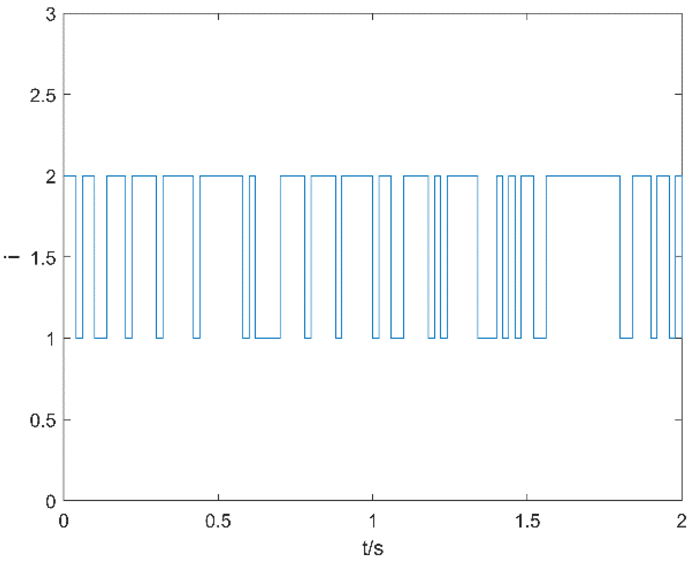
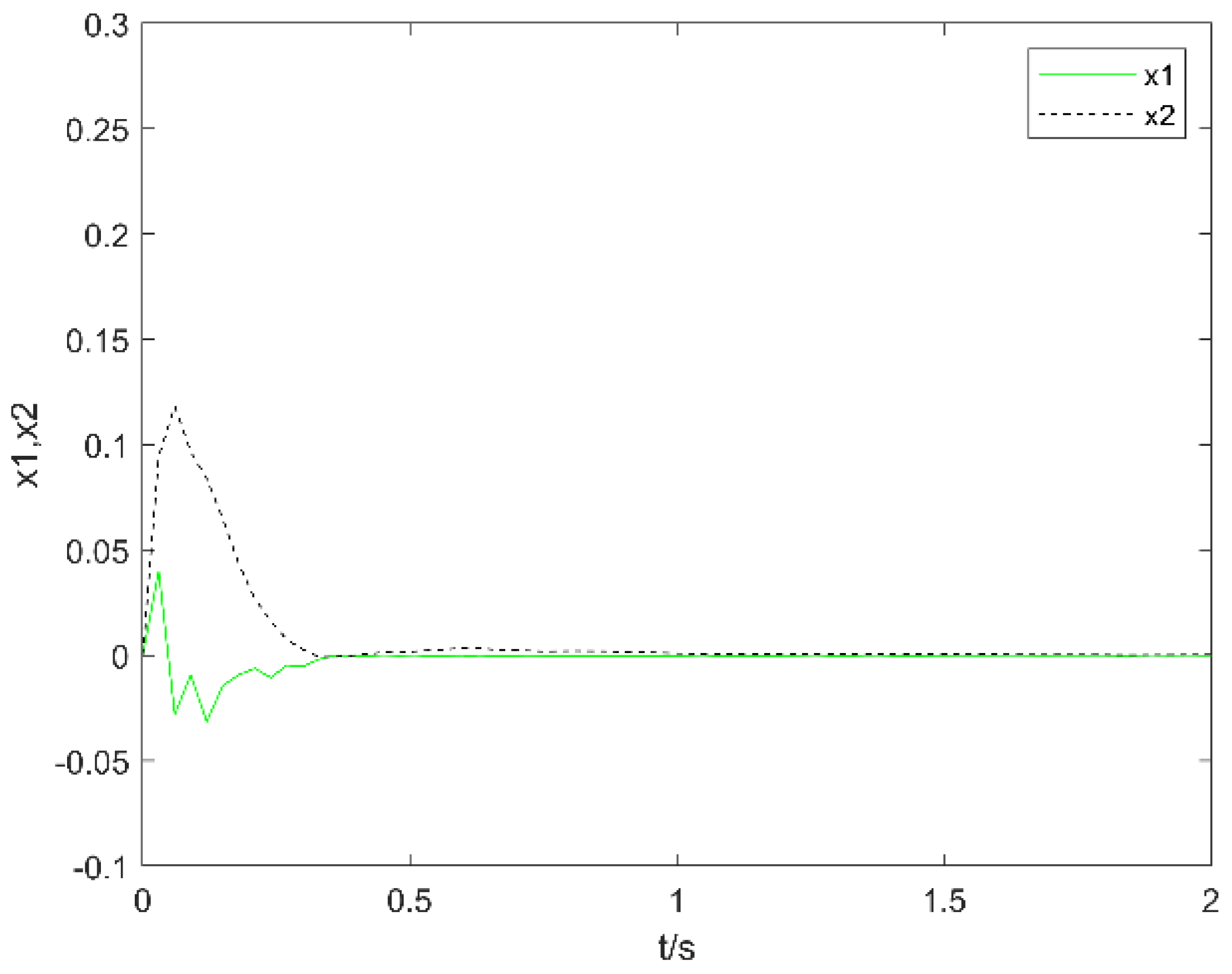
4. Numerical Example

In this section, an example is used to show the effectiveness of the controller presented.

Consider the following RLC electric circuit [33]

$$H\ddot{Q}\left(t\right)-\dot{Q}\left(t\right)+\frac{1}{\mathbb{C}}Q\left(t\right)=G\left(t\right)\dot{W}\left(t\right)$$

(33)

where H is the inductance, $Q\left(t\right)$ is the charge, $\mathbb{C}$ is the capacitance, $\dot{W}\left(t\right)$ is one-dimensional white noise and $G\left(t\right)$ is the intensity of the noise. Suppose that system (33) experiences abrupt changes and its parameters switch from one to another. Then, (33) is represented by

$$H_{\eta \left(t\right)}\ddot{Q}\left(t\right)-\dot{Q}\left(t\right)+\frac{1}{{\mathbb{C}}_{\eta \left(t\right)}}Q\left(t\right)=G_{\eta \left(t\right)}\left(t\right)\dot{W}\left(t\right)$$

(34)

where $\eta \left(t\right)$ is a Markov process taking values in $\overline{L}=\{1,2\}$.

Let $x\left(t\right)={\left[\begin{array}{cc}{x}_1\left(t\right)& x_2\left(t\right)\end{array}\right]}^{\prime }={\left[\begin{array}{cc}Q\left(t\right)& \dot{Q}\left(t\right)\end{array}\right]}^{\prime }$, and then (34) is rewritten as Itô MJSs

$$\left\{\begin{array}{c}\hfill \begin{array}{cc}\hfill d{x}_1\left(t\right)& =x_2\left(t\right)dt,\hfill \\ \hfill d{x}_2\left(t\right)& =\frac{1}{H_{\eta \left(t\right)}}[x_2\left(t\right)-\frac{1}{{\mathbb{C}}_{\eta \left(t\right)}}{x}_1\left(t\right)]dt+\frac{G_{\eta \left(t\right)}\left(t\right)}{H_{\eta \left(t\right)}}dW\left(t\right).\hfill \end{array}\end{array}\right.$$

(35)

We introduce a control device, and then (35) is expressed as

$$\left\{\begin{array}{c}\hfill \begin{array}{cc}\hfill d{x}_1\left(t\right)& =[x_2\left(t\right)+{\alpha }_{1\eta \left(t\right)}u\left(t\right)]dt,\hfill \\ \hfill d{x}_2\left(t\right)& =\frac{1}{H_{\eta \left(t\right)}}[x_2\left(t\right)-\frac{1}{{\mathbb{C}}_{\eta \left(t\right)}}{x}_1\left(t\right)+{\alpha }_{2\eta \left(t\right)}u\left(t\right)]dt+\frac{{\beta }_{\eta \left(t\right)}x\left(t\right)}{H_{\eta \left(t\right)}}dW\left(t\right).\hfill \end{array}\end{array}\right.$$

That is,

$$dx\left(t\right)=[A_{\eta \left(t\right)}x\left(t\right)+B_{\eta \left(t\right)}u\left(t\right)]dt+C_{\eta \left(t\right)}x\left(t\right)dW\left(t\right)$$

where $A_{\eta \left(t\right)}=\left[\begin{array}{cc}0& 1\\ -\frac{{\mathbb{C}}_{\eta \left(t\right)}}{H_{\eta \left(t\right)}}& \frac{1}{H_{\eta \left(t\right)}}\end{array}\right]$, $B_{\eta \left(t\right)}=\left[\begin{array}{c}{\alpha }_{1\eta \left(t\right)}\\ {\alpha }_{2\eta \left(t\right)}\end{array}\right]$ and $C_{\eta \left(t\right)}=\left[\begin{array}{cc}0& 0\\ 0& \frac{{\beta }_{\eta \left(t\right)}}{H_{\eta \left(t\right)}}\end{array}\right]$.

Due to the unavoidable finite switching speed of amplifiers, a time delay inevitably exists in an electric circuit. Moreover, the electric energy consumption is expected to be minimal. Based on the above, we consider the time-delay Itô MJSs described by (1) and cost performance (2), whose parameters are given below.

Mode 1:

$$\begin{array}{c}{A}_1=\left[\begin{array}{cc}0& 1\\ -2.2& 1.5\end{array}\right],{\overline{A}}_1=\left[\begin{array}{cc}-1& -0.21\\ 0& -1\end{array}\right],B_1=\left[\begin{array}{c}1.6\\ -0.5\end{array}\right],C_1=\left[\begin{array}{cc}0& 0\\ 0& -0.1\end{array}\right],\hfill \\ {\overline{C}}_1=\left[\begin{array}{cc}-0.02& 0.1\\ 0.1& 0.1\end{array}\right],Q_{11}=\left[\begin{array}{cc}0.5& 0\\ 0& 0.5\end{array}\right],Q_{21}=1.\hfill \end{array}$$

Mode 2:

$$\begin{array}{c}{A}_2=\left[\begin{array}{cc}0& 1\\ -3& 1.5\end{array}\right],{\overline{A}}_2=\left[\begin{array}{cc}1& -0.5\\ 0.3& -0.9\end{array}\right],B_2=\left[\begin{array}{c}5\\ 0.2\end{array}\right],C_2=\left[\begin{array}{cc}0& 0\\ 0& -0.2\end{array}\right],\hfill \\ {\overline{C}}_2=\left[\begin{array}{cc}-0.2& 0.12\\ 0.2& -0.1\end{array}\right],Q_{12}=\left[\begin{array}{cc}0.7& 0\\ 0& 0.7\end{array}\right],Q_{22}=1.\hfill \end{array}$$

Moreover, $\overline{d}=0.1,\tilde{d}=1,\tilde{T}=2,c_1=0.3,{ϵ}_1=0.6,{ϵ}_2=1,\rho =1,x\left(t\right)={[x_1\left(t\right),x_2\left(t\right)]}^T,x\left(0\right)={\left[00\right]}^T$, $R=I$. The transition rate matrix

$$\mathcal{Q}=\left[\begin{array}{cc}-0.85& 0.85\\ 1.6& -1.6\end{array}\right].$$

One possible Markovian mode evolution for $\eta \left(t\right)=i$ is shown in Figure 1.

From Theorem 3, the feasible solution can be found when $\gamma \in (0,10.3)$. The minimum of $c_2$ is $13.02$ when $\gamma =0$. The corresponding controller gains $K_1=\left[4.490.24\right],K_2=[-0.480.05]$. The minimum value of the guaranteed cost upper bound for (5) is ${\mathcal{J}}^{*}=0.67$. This shows that controllers $u\left(t\right)=K_{1}x\left(t\right)$ and $u\left(t\right)=K_{2}x\left(t\right)$ are state feedback finite-time guaranteed cost controllers for system (4).

The state responses of $x_1\left(t\right)$ and $x_2\left(t\right)$ are shown in Figure 2, which implies that the state trajectories of system (4) are bounded. The evolution of $\mathcal{E}\left[x^T\left(t\right)Rx\left(t\right)\right]$ for system (4) is depicted in Figure 3, where it is obvious that $\mathcal{E}\left[x^T\left(t\right)Rx\left(t\right)\right]<c_2$, which means that the closed-loop system (4) is finite-time stable with respect to $(0.3,13.02,2,I)$.

5. Conclusions

We have considered the FTGCC problem for MJSs with time-varying delays. Finite-time guaranteed cost controllers are designed, which ensure the finite-time stability of closed-loop systems and an upper bound of cost performance. The effectiveness of the main results has been shown by an example. In this paper, transition rates are assumed to be completely known for MJSs. However, they may be partially known or fully unknown. The results obtained can be extended to FTGCC for MJSs with time-varying delays and generally uncertain transition rates. In the future, the problem of finite-time $H_{\infty }$ control will be developed for MJSs with time-varying delays.

References

1. Aberkane, S.; Dragan, V. H filtering of periodic Markovian jump systems: Application to filtering with communication constraints. Automatica 2012, 48, 3151–3156. [Google Scholar] [CrossRef]
2. Kazemy, A.; Hajatipour, M. Event-triggered load frequency control of Markovian jump interconnected power systems under denial-of-service attacks. Int. J. Electr. Power Energy Syst. 2021, 133, 107250. [Google Scholar] [CrossRef]
3. Huo, S.; Zhang, Y. H consensus of Markovian jump multi-agent systems under multi-channel transmission via output feedback control strategy. ISA Trans. 2020, 99, 28–36. [Google Scholar] [CrossRef] [PubMed]
4. Jiang, P.; Zhu, J.; Xi, H. Stability and stabilization for non-homogeneous positive Markovian jump linear systems. Control Theory Appl. 2020, 37, 229–235. [Google Scholar] [CrossRef]
5. Chen, L.; Shi, P.; Liu, M. Fault reconstruction for Markovian jump systems with iterative adaptive observer. Automatica 2019, 105, 254–263. [Google Scholar] [CrossRef]
6. Song, J.; Niu, Y.; Zou, Y. Asynchronous sliding mode control of Markovian jump systems with time-varying delays and partly accessible mode detection probabilities. Automatica 2018, 93, 33–41. [Google Scholar] [CrossRef]
7. Liu, X.; Zhang, W.; Li, Y. H-index for continuous-time stochastic systems with Markov jump and multiplicative noise. Automatica 2019, 105, 167–178. [Google Scholar] [CrossRef]
8. Li, Y.; Zhang, W.; Liu, X. H-index for discrete-time stochastic systems with Markovian jump and multiplicative noise. Automatica 2018, 90, 286–293. [Google Scholar] [CrossRef]
9. Amato, F.; Ambrosino, R.; Ariola, M.; Cosentino, C.; De Tommasi, G. Finite-Time Stability and Control; Springer: London, UK, 2014. [Google Scholar] [CrossRef]
10. Dorato, P. Short time stability in linear time-varying systems. In Proceedings of the IRE International Convention Record Part 4, New York, NY, USA, 9 May 1961; Volume 4, pp. 83–87. [Google Scholar]
11. Amato, F.; Ariola, M.; Dorato, P. Finite-time control of linear systems subject to parametric uncertainties and disturbances. Automatica 2001, 37, 1459–1463. [Google Scholar] [CrossRef]
12. Amato, F.; Ambrosino, R.; Ariola, M.; De Tommasi, G. Robust finite-time stability of impulsive dynamical linear systems subjective to norm-bounded uncertainties. Int. J. Robust Nonlinear Control 2011, 21, 1080–1092. [Google Scholar] [CrossRef]
13. Amato, F.; Ariola, M.; Cosentino, C. Finite-time stability of linear time-varying systems: Analysis and controller design. IEEE Trans. Autom. Control 2010, 55, 1002–1008. [Google Scholar] [CrossRef]
14. Amato, F.; Ambrosino, R.; Ariola, M.; De Tommasi, G.; Pironti, A. On the finite-time boundedness of linear systems. Automatica 2019, 107, 454–466. [Google Scholar] [CrossRef]
15. Mu, X.; Li, X.; Fang, J.; Wu, X. Reliable observer-based finite-time H control for networked nonlinear semi-Markovian jump systems with actuator fault and parameter uncertainties via dynamic event-triggered scheme. Inf. Sci. 2021, 546, 573–595. [Google Scholar] [CrossRef]
16. Tartaglione, G.; Ariola, M.; Cosention, C.; De Tommasi, G.; Pironti, A.; Amato, F. Annular finite-time stability analysis and synthesis of stochastic linear time-varying systems. Int. J. Control 2021, 94, 2252–2263. [Google Scholar] [CrossRef]
17. Tartaglione, G.; Ariola, M.; Amato, F. Conditions for annular finite-time stability of Itô stochastic linear time-varying syetems with Markov switching. IET Control Theory Appl. 2019, 14, 626–633. [Google Scholar] [CrossRef]
18. Gholami, H.; Shafiei, M. Finite-time H static and dynamic output feedback control for a class of switched nonlinear time-delay systems. Appl. Math. Comput. 2021, 389, 125557. [Google Scholar] [CrossRef]
19. Yan, Z.; Zhang, W.; Zhang, G. Finite-time stability and stabilization of Itô stochastic systems with Markovian switching: Mode-dependent parameter approach. IEEE Trans. Autom. Control 2015, 60, 2428–2433. [Google Scholar] [CrossRef]
20. Yan, Z.; Song, Y.; Liu, X. Finite-time stability and stabilization for Itô-type stochastic Markovian jump systems with generally uncertain transition rates. Appl. Math. Comput. 2018, 321, 512–525. [Google Scholar] [CrossRef]
21. Li, Z.; Xu, Y.; Fei, Z.; Huang, H.; Misra, S. Stability analysis and stabilization of Markovian jump systems with time-varying delay and uncertain transition information. Int. J. Robust Nonlinear Control 2018, 28, 68–85. [Google Scholar] [CrossRef]
22. Wang, G.; Li, L.; Zhang, Q.; Yang, C. Robust finite-time stability and stabilization of uncertain Markovian jump systems with time-varying delay. J. Frankl. Inst. 2017, 293, 377–393. [Google Scholar] [CrossRef]
23. Bai, Y.; Sun, H.; Wu, A. Finite-time stability and stabilization of Markovian jump linear systems subject to incomplete transition descriptions. Int. J. Control Autom. Syst. 2021, 19, 2999–3012. [Google Scholar] [CrossRef]
24. Petersen, I. Guaranteed cost control of stochastic uncertain systems with slop bounded nonlinearities via the use of dynamic multipliers. Automatica 2011, 47, 411–417. [Google Scholar] [CrossRef]
25. Li, L.; Zhang, Q.; Zhu, B. Fuzzy stochastic optimal guaranteed cost control of bio-economic singular Markovian jump systems. IEEE Trans. Cybern. 2015, 45, 2512–2521. [Google Scholar] [CrossRef] [PubMed]
26. Qayyum, A.; Pironti, A. On finite-time stability with guaranteed cost control of uncertain linear systems. Kybernetika 2018, 54, 1071–1090. [Google Scholar] [CrossRef]
27. Yan, Z.; Zhang, G.; Wang, J.; Zhang, W. State and output feedback finite-time guaranteed cost control of linear Itô stochastic systems. J. Syst. Sci. Complex. 2015, 28, 813–829. [Google Scholar] [CrossRef]
28. Yan, Z.; Park, J.; Zhang, W. Finite-time guaranteed cost control for Itô stochastic Markovian jump systems with incomplete transition rates. Int. J. Robust Nonlinear Control 2017, 27, 66–83. [Google Scholar] [CrossRef]
29. Liu, X.; Liu, Q.; Li, Y. Finite-time guaranteed cost control for uncertain mean-field stochastic systems. J. Frankl. Inst. 2020, 357, 2813–2829. [Google Scholar] [CrossRef]
30. Yan, Z.; Song, Y.; Park, J. Finite-time H2/H control for linear Itô stochastic Markovian jump systems: Mode-dependent approach. IET Control Theory Appl. 2020, 14, 3557–3567. [Google Scholar] [CrossRef]
31. Oksendal, B. Stochastic Differential Equations: An Introduction with Applications, 5th ed.; Springer: New York, NY, USA, 2000. [Google Scholar] [CrossRef]
32. Ouellette, D. Schur complements and statistics. Linear Algebra Appl. 1981, 36, 187–295. [Google Scholar] [CrossRef]
33. Mao, X.; Yuan, C. Stochastic Differential Equations with Markovian Switching; Imperial College Press: London, UK, 2006. [Google Scholar] [CrossRef]
Figure 1. One possible Markovian mode evolution.
Mathematics 10 02028 g001
Figure 2. The state responses for system (4).
Mathematics 10 02028 g002
Figure 3. The evolution of E [ x T ( t ) R x ( t ) ] for system (4).
Mathematics 10 02028 g003
Publisher’s Note: MDPI stays neutral with regard to jurisdictional claims in published maps and institutional affiliations.