Abstract
Electricity price forecasting has been a booming field over the years, with many methods and techniques being applied with different degrees of success. It is of great interest to the industry sector, becoming a must-have tool for risk management. Most methods forecast the electricity price itself; this paper gives a new perspective to the field by trying to forecast the dynamics behind the electricity price: the supply and demand curves originating from the auction. Given the complexity of the data involved which include many block bids/offers per hour, we propose a technique for market curve modeling and forecasting that incorporates multiple seasonal effects and known market variables, such as wind generation or load. It is shown that this model outperforms the benchmarked ones and increases the performance of ensemble models, highlighting the importance of the use of market bids in electricity price forecasting.
Keywords:
electricity price forecast; electricity; market curves; electricity price; vector auto regression; time-series MSC:
62H12; 62M10; 91B84; 91-10
1. Introduction
Energy markets are commodity markets that deal exclusively with the supply and trade of energy, which can refer to electricity or any other source of energy.
Electricity stands out from other commodities because it has specific physical and economic characteristics. You cannot see, smell or touch it, and you cannot even guarantee its motion from one point to another in the same way as other commodities all because of the complex physics laws that govern it. It is economically non-storable, and the power system requires a constant balance between production and consumption. At the same time, its demand and production are dependent on many changeable variables, such as temperature, wind speed or solar radiation, or even the hours of the day or the days of the week where business and everyday activities are more intense. These unique characteristics lead to a very volatile market of high importance for governments, industry and consumers, with price dynamics that are not observable in any other market.
In the current deregulated scenario, the forecasting of electricity price has emerged as one of the major research fields [1]. The liberalization was intended to encourage competition among companies to decrease the cost of electricity. Unfortunately, occurrences that were of no concern in the regulated market, such as outages, possible blackouts and price peaks are now subjects of increasing concern. Moreover, deregulation increases electricity price uncertainty, giving an increased role to forecasting.
Precision in forecasting these electricity prices is very important, since a higher accuracy reduces the risk of under- or overestimating the revenue from the production units for the companies and provides better risk management [2]. Forecast errors have significant implications for profits, market shares and ultimately shareholder value [1]. In actual electricity markets, the price curve exhibits a rich structure that has the following characteristics: high frequency, nonconstant mean and variance, multiple seasonality, calendar effect, high level of volatility and high percentage of unusual price movements. These characteristics arise from the properties of the electricity and also from the fact that the market equilibrium is influenced by both the load and the generation side uncertainties [1]. Therefore, electricity price forecasting is essential for all market participants for their survival. In the short-term, a producer needs to forecast electricity prices to be able to formulate its bidding strategy and to optimally schedule its electric energy resources [3]. In a regulated environment, traditional generation scheduling of energy resources was based on cost minimization, satisfying the electricity demand and all operating constraints [4], and therefore, the key issue was how to accurately forecast electricity demand. In a deregulated environment, since generation scheduling of energy resources, such as hydro [5] and thermal resources [6], is now based on profit maximization [7], it is accurate price forecasting that embodies crucial information for any decision making.
Over the last years, different methods and approaches have been tried for electricity price forecasts with varying degrees of success. The increasing number of studies published has been highly motivated not only by industry sector needs, but also by the challenges that the electricity markets present.
The electricity price is obtained from the demand and supply curves in a daily hourly auction, being the direct result of the supply fulfilling the demand. However, most electricity price forecasting approaches tend to overlook these underlying effects, using only market variables such as load or renewable generation forecasts. We strongly believe that the market curves give crucial information for the price formation and therefore, should be included in the forecasting models. In particular, the main contributions of this paper are:
- Introduction of a novel method for market offers forecasting, by modeling market curves, and a way of predicting electricity price from them;
- Market curve forecasting through parameter analysis, including correlation with other market variables, multiple seasonal effects derived from spectrum analysis and vector autoregression techniques;
- Analysis of the performance of the proposed model, showing that the market curves give information that is not captured through other variables, highlighting the importance of using market offers in future models.
2. The Day-Ahead Market
The liberalization and reorganization of the electric sector changed the way generation and supplier companies interact, bringing about the need for regulated markets. One of the mechanisms that was created is spot markets, know as pool markets (because it includes all the producers and suppliers of the system), with the primary objective of achieving a balance between production and demand. The day-ahead markets are the main object of the spot-markets, so named because they take place the day before the scheduled power delivery. They help optimize the system in the short term by making it easier for generation companies to correctly schedule their units, specifically their slower-start units [8,9].
The day-ahead market is based on a sealed-bid auction, typically a uniform price auction (UPA). The UPA is a kind of sealed-bid auction that does not discriminate the price over the different players and incentivizes the use of marginal price as the base for the competitive pricing. In UPA, all of the winners would be paid at a single predetermined price, namely the market clearing price (MCP), irrespective of what they had bid, and the last winning bidder, which is called the marginal unit, will get exactly the bid price. The pricing rule and the whole process of clearing the market is simple and straightforward; it is based on the equilibrium between production and demand. The independent system operator aggregates the supply offers and demand bids and arranges them in the form of ascending and descending curves. The intersection of these two curves will determine the market price and the cleared quantity, as seen in Figure 1 [10].
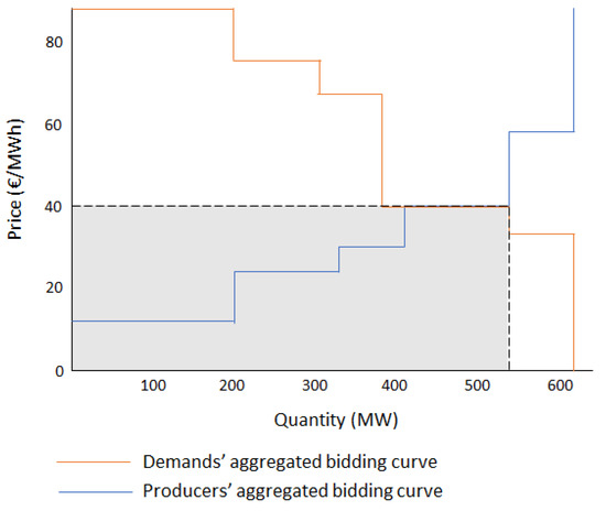
Figure 1.
Uniform price auction clearing illustration.
3. Electricity Price Forecasting
Despite the increasing interest, the large amount of electricity markets and their different complexity make it difficult to compile all the existing models in the literature and compare them with each other. Market configuration has a high influence in the final clearing price since different electricity markets around the world have different caps and floors in the electricity price. Moreover, the number of available additional markets, such as capacity, balancing or ancillary services, will change the way agents make their offers and thus, change the electricity price in the day-ahead market. In addition, geographical characteristics play a major role. The generation mix or grid design of each market is enough to completely alter the performance of the models when applied to different markets.
The MCP is obtained from all demand and supply offers in an organized auction. The main reason behind this auction is the the system operators requiring advance notice to verify that the schedule is feasible and falls within transmission constraints. This auction happens once a day and results in prices for all periods of the following day (typically 24 h).
This means that when forecasting or modeling the day-ahead market, one has to take into account that all 24 prices for the next day are determined at the same time and thus, have the same market information. There are two interesting effects that result from this: first, the dynamics of hourly price does not behave as a univariate pure time series process, instead, these prices may be seen as daily arrays of 24 h [11]. They only approximate a time series because most of the underlying dynamics in the bids are in fact univariate time series (demand, wind production, solar production, etc.). Second, the prices have no relation to the real values observed in the electrical system load or renewable energy generation but instead are highly dependent on what the market foresaw as expected for the next day. This means that forecasts of these variables will work better as exogenous variables for the models than the actual observed values.
Regarding predictive models, most of the literature refers to point forecasts, where the target is the actual day-ahead price. The point forecast can be obtained using different techniques by modeling the hourly price in the past and forecasting or by simulating the supply and demand curve for the next hours and obtaining the price by intercepting both curves. Nevertheless, models where the demand and supply curves are the object of modeling are still to be found among the main EPF authors and journals.
Electricity price forecasts models can be separated into four distinct families: Statistical, Fundamental, Machine Learning and Hybrid. Statistical models are quite common in the literature and come from the direct application of statistical techniques. They include regression type models, autoregressive type time series models and reduced-form models (Figure 2).
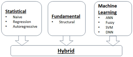
Figure 2.
Diagram of electricity price forecasting method families.
Fundamental models try to describe the price dynamics by modeling important physical and economic factors and simulating the operation of a system of heterogeneous agents interacting with each other. Although favored in the industry sector, these models are often used for mid- or long-term forecasts, as they perform poorly in the short-term.
Machine learning are models which combine elements of learning, evolution and fuzziness to create approaches that are capable of capturing complex dynamic systems. There has been an increased interest in machine learning models because of their capability to capture nonlinear behaviour.
Finally, hybrid models try to combine two or more techniques from the other families for EPF. They have increased in popularity because of their ability to capture the pros of different models, minimizing the cons. Since their classification is almost impossible, they have a family of their own.
3.1. Statistical Models
Historically, the first statistical EPF techniques consisted of replicating statistical methods of load forecasting. By a simple substitution of loads or temperatures for electricity prices, the researchers were able to obtain EPF models. As time passed, more and more contemporary statistical, econometric or signal processing techniques were introduced to this area.
Statistical methods forecast the current price by using a mathematical combination of the previous prices and exogenous factors, typically consumption and production figures, or weather variables.
Most models in this family rely on linear regression and represent the target variable, i.e., the price for time (hour) h, by a linear combination of independent variables (the predictors):
where is a vector of coefficients specific to hour h, is a vector of inputs and is an error term.
In most EPF papers, the author refers to a benchmark model. It is based on searching historical data for a day with similar characteristics to the predicted day and using this historical value as a forecast for the future. The most common application was introduced by [12] and is called the naïve method. The procedure is so basic that it has been extensively used in the literature for comparison purposes. If your method cannot outperform the naïve, then it is simply not good enough. The procedure consists of taking the day of the week from the previous week and applying it to the next one. This way a Monday will be equal to last Monday, a Tuesday to last Tuesday, and so on.
In addition to this approach, most statistical models consist of multiple regressions, aiming to learn more about the relationships between several independent or predictor variables and a dependent or criterion variable.
Regression models are so common and popular in EPF that it is almost impossible to make a full review on all of them. Moreover, most papers use regression models combined with some other methods, normally more sophisticated. It is also hard to separate regression and autoregressive models since most of them use some kind of lagged electricity price as regressors.
In the last few years, the most relevant contribution to EPF has been the appearance of linear regression with a large number of input features that utilize some kind of regularization technique. If the number of regressors is too large, using least absolute shrinkage and selection operator (LASSO) or the elastic net limits them. By using a penalty factor jointly with minimizing the residual sum of squares (RSS), one can turn some of the coefficients to zero and effectively eliminate redundant regressors. These regularized regression models exhibit superior performance [12,13,14,15,16,17,18].
Another innovation in this family is the use of different calibration windows on the same model and combining them afterwards. It was shown that this approach outperforms the predictions obtained for the best ex post selected calibration window [19,20].
Autoregressive models take into account the time correlations of the data we are studying. The is expressed linearly in terms of its p past values (autoregressive parameter), and in terms of q values of the noise (moving average part):
where B is the backward shift operator , is the notation for , and is a notation for , where and are the coefficients of the model. This is called the AutoRegressive Moving Average model and it is stylized ARMA().
This model composes a family of its own because many variations can be built: ARIMA, SARIMA or ARMAX. The first includes a differentiating term to ensure stationarity; the second adds a seasonal component of period s, and the latter includes exogenous variables in the model.
Autoregressive-type models represent the backbone of all time series models of electricity prices and have been widely used. The authors of [21] successfully use an AR model, with lags of 24, 48 and 168 h, where each hour of the day is modeled separately, to account for residual autocorrelation and seasonal dynamics, with the inclusion of load forecasts, and use it for short-term EPF.
Similar to this approach, the authors of [22] propose a set of 24 h ARIMA models for weekdays (which are calibrated only to weekday prices) and a set of 24 h ARIMA models for weekends (which are calibrated to weekday and weekend prices).
Wavelet-ARIMA techniques that consist of decomposing the price series using a discrete wavelet transform, modeling the resulting detail and approximation series using ARIMA processes to obtain 24 hourly predicted values, and then applying the inverse wavelet transform to yield the predicted prices for the next 24 hours have been proposed by [23,24]. The performance of the wavelet-ARIMA technique is generally better than that of a standard ARIMA process.
An interesting methodology which combines elements of time series and multi-agent modeling has been described in [25]. They forecast 24 h prices for the next day using an ARIMA model applied to the conjectural variations of the firms participating in the Spanish power market. They find that this model performs slightly better than a pure ARIMA model.
Most recent constructions of ARIMA models in the literature have been used as benchmarks for more complex machine learning models.
Statistical models are attractive because some physical interpretation may be taken from their results, thus allowing the user to understand their behavior. They are often criticized for their limited ability to model the nonlinear behavior of electricity prices and related fundamental variables; nonetheless, in practical applications, their performances are comparable to those of their nonlinear alternatives.
3.2. Fundamental Models
The next class of models, known as fundamental or structural models, tries to capture the basic physical and economic relationships which are presented in the day-ahead market. The functional associations between fundamental drivers (loads, weather conditions, system and power plant parameters, etc.) are theorized, and the fundamental inputs are modeled and predicted independently, often via statistical or machine learning techniques. Many of the EPF approaches considered in the literature are hybrid solutions with time series, regression and neural network models using fundamental factors, such as loads, fuel prices, wind power or temperature, as input variables.
Many of these models are often developed as proprietary; therefore, their details are not disclosed publicly. In fact, one can find several providers of software for long-term EPF with parameter-rich fundamental models. At the academic level, most of the results published relate to hydro-dominant power markets, since the functional behavior of hydropower plants bidding is easier to emulate in these models than with statistical ones. In particular, the authors of [26] present a supply–demand model for the Norwegian power market from a time before the common Nordic market (Nordpool) had started. He uses hydro-inflow, snow and temperature conditions to explain spot price formation.
The authors of [27] use a fundamental model that aims to simulate the market-clearing process by minimizing the total system costs, which are constrained by generation unit technical features, regulation limits, transmission limits and the demand vs. generation balance. Thus, in this model, the estimated electricity market price can be obtained as the dual variable of the demand balance constraint. The forecast clearing price is then used as input to a neural network model to obtain the final electricity price forecasting.
Under the fundamental models, there is a subclass of simpler structural models that can be built from empirical analysis of market supply and demand curves. The first approach made consists of building the day-ahead spot price process by applying the inverse of the Box–Cox transformation to an Ornstein–Uhlenbeck process [28].
A similar approach can be seen in [29], where the authors define a hockey-stick shaped supply curve that matches the empirically observed curves better than the inverse of the Box–Cox transformation. They combine this with an inelastic vertical demand curve with horizontal stochastic variations driven from and Ornstein–Uhlbeck process.
3.3. Machine Learning Models
Machine learning is the study of computer algorithms and techniques to make decisions or predictions by the use of data. Is a very diverse group that has been developed to solve problems which traditional methods (e.g., statistical) cannot handle efficiently. It combines elements of learning, evolution and fuzziness to create approaches that are capable of capturing complex nonlinear dynamic systems and because of that are regarded as ‘intelligent’.
From all the machine learning, artificial neural networks (ANN), fuzzy systems, support vector machines (SVM) and evolutionary computation, are definitely the main classes. These models are sophisticated and flexible enough to handle complex systems and nonlinearity. This makes them very promising for short-term EPF, especially in complex markets with effects from varied sources. Although artificial neural networks have probably received the most attention, other non-parametric techniques, such as fuzzy logic, genetic algorithms, evolutionary programming and swarm intelligence, have also been applied, but typically in hybrid constructions.
With the increase of computational power available to the common user, in the last six years there has been a growing interest in deep neural networks, a neural network with a more complex structure with several hidden layers. However, despite this trend, most of the published studies are quite limited, with poor benchmarks, and they usually avoid state-of-the-art statistical methods.
ANN models have been widely employed in EPF. One output node has been used to forecast the next hour’s price [30,31], the price h hours ahead [32,33,34], the next day’s peak price [35], the next day’s average on-peak price [36] or the next day’s average baseload price [37]. Using models with several output nodes, it is possible to forecast a vector of prices, typically 24 nodes for forecasting the next day’s complete price profile [38].
Multi-layer perceptron (MLP) has also been used in EPF, as it proved to be good at capturing global data trends [34,39,40,41]. A model with a hybrid system has been proposed in [42], in which a real-coded genetic algorithm (RCGA) with an enhanced stochastic search capability is used to train an MLP. The authors show that this method can provide more accurate results for the Spanish market than a standard ARIMA model, a wavelet-ARIMA model or a fuzzy ANN.
More recently, recurrent neural networks (RNN) have been employed for electricity price. The authors of [43] employ two recurrent networks, one for time-positive forward data processing, and another for negative time-backward real prices processing. In another study, an RNN is used, in particular an LSTM, for calculating electricity prices for each hour [44].
In electricity price forecasting, SVMs are normally seen in hybrid models. However, in one of the first papers on this topic, an MLP and an SVM are compared with exactly the same inputs and conclude that the SVM has a more consistent behavior while requiring less time for optimal training [45]. A hybrid model called SVRARIMA that combines support vector regression to capture the nonlinear patterns and ARIMA models outperforms some of the existing ANN approaches and traditional ARIMA models [46].
Fuzzy logic has also been applied to EPF. One of the first applications utilizes fuzzy-c-means for classifying historical data into three distinct clusters representing peak, medium and off-peak and then employs an ANN for forecasting [47,48]. An adaptive-network-based fuzzy inference system (ANFIS) can be seen in [34], which combines an adaptive mechanism with Sugenotype rules and uses a combination of the least squares method and back-propagation for training the membership function and the linear combination parameters. They show that the ANFIS performs better than an MLP.
However, the most recent evolution on EPF has been in deep learning. Deep learning is a family of machine learning methods closely related to artificial neural networks, in which several layers of neurons are used, hence the name “deep”. The existence of many layers allows for the search of more features in the input data since each layer can identify different signals.
The first published deep learning paper [49] proposes a deep learning network using stacked denoising autoencoders. The new method is compared against machine learning techniques but also against two statistical methods. Four DL models (a DNN, two recurrent neural networks (RNNs), and a convolutional network (CNN)) were developed, and the results between them were compared using a whole year of data against a benchmark of 23 different models, including 7 machine learning models, 15 statistical methods and a commercial software [15]. Moreover, among the statistical methods, the comparison includes the fARX-Lasso and fARX-EN which are among the state-of-the-art statistical methods. The study showed that the deep learning algorithms perform slightly better than the others.
Deep learning became popular buzzwords, being the techniques seen as the state of the art. However, they impose a severe computational burden, their relative performance is not well tested and the training process is described by many hyper-parameters in which the optimal values are unknown, thus requiring a lot of effort to tune and apply.
3.4. Hybrid
Within the field of EPF, the research area that had the biggest contribution has been hybrid forecasting methods. They also have the most recent contributions in the literature. In fact, most of the approaches already discussed here are actually hybrid in some sense.
Hybrid models are very complex forecasting frameworks that are composed of several algorithms and techniques. Usually, they comprise different models for different components or modules of a forecasting technique, which can be data decomposition [50,51,52,53,54,55], feature selection [52,56,57,58,59,60], data clustering [59,61,62,63], some heuristic optimization of hyperparameters [50,55,57,58,64,65,66,67] or prediction ensemble [68,69,70,71].
3.5. Industry Sector Applications
There is a significant discrepancy between the recent advances in EPF at an academic level and at an industrial level. In fact, despite all the models that have been developed and published by the academy, most models used for industry application are much simpler. This is understandable as the industry sector has different objectives from the academy.
Most of the models discussed are complex, hard to optimize and computation heavy. If the companies require fast inputs for decision making, it becomes hard to use these models on a daily basis. It also requires a specific level of expertise to be able to correctly tune and maintain most models, especially artificial neural networks and deep learning models, which may be hard (and expensive) to find. Moreover, because of the lack of a common framework for studying and benchmarking EPF models, it becomes unclear for decision makers if the time and money needed will have the expected return. Nonetheless, EPF is of major importance in the industry sector and requires constant investment.
The most-used models in the industry sector are statistical models, in particular autoregressive dynamic models, which are an extension of the ARIMA models where the exogenous variable is also a time series forecast. In this case, the use of lagged values for the exogenous variable improves the performance of the overall model. Using the notation introduced in Section 3 we can write the model as:
A curious fact about this model (and most statistical ones) is that the number of exogenous or explanatory variables V used can affect the model performance. A model with fewer exogenous variables performs better than one that uses all possible explanatory variables, mostly because of high colinearity between the variables. Because of that, there are a significant number of different models with different exogenous variables. These have been the motivation for the development of new hybrid methods that focus on regressor selection already discussed and the need to develop techniques for forecast selection or ensemble.
The difficulty found in choosing the right model for the right situation raised the need for methods that combined forecasts with the most-used approach being the ensemble averaging. Although ensemble averaging had the advantages of minimizing the risk of having a poor forecast (it is never as bad as the worst available single forecast), it also makes it impossible to have the best forecast possible (it is always worse than the best single forecast available). The pursuit of a method that could lead to the best average possible while minimizing the risk of making a poor forecast led to new techniques, in particular the use of random forests and XGBOOST algorithms to “correct” the forecast errors obtained from statistical methods. In these approaches, the statistical models predictions are used as inputs for the random forests or gradient boosting models which in turn outputs new forecasts that are slightly better than the simple average.
In addition to these methods, it is also common to see simple artificial neural network machine learning models employed in the companies, such as single-layer perceptrons or support vector machines. However, the performance of these models when compared to statistical ones is not clear. Statistical models are usually preferred over machine learning because they are easier to interpret and help in fundamental market analysis.
There is still a relevant gap in the companies needs that today’s models still fail to meet. To optimize the bidding strategy for some production units, such as hydro-reservoirs, the price forecast might not be enough. We also need to know the price sensitivity with over- or undersupply. Despite its importance to the companies, this approach is disregarded by academia, mainly because of the lack of visibility over company assets and its valuation. The method and methodology described in this paper aims to fulfill that gap by introducing a new market curve forecast model.
4. Methodology
Apart from a small family of models (fundamental/structural), most of the EPF approaches focus on studying the electricity price as a vector of single hourly observations. These observations can then be studied as a time series, and all the known techniques are available for analysis and forecasting. The prediction methods tend to disregard that there is an actual physical structure behind the price, i.e., the price is a consequent construction of a series of offers that the agents make in an organized market. This means that the electricity price is not the unknown; the real unknowns are the bids/asks (or the market curves) by themselves. If you knew all the bids for the future, we could accurately infer the electricity prices.
From an industry sector point of view, the forecast of the supply and demand curves brings many advantages when compared to simple price forecasts. You can derive different measures by looking at the curves and obtaining information impossible to get otherwise, such as: (i) price sensitivity—how will the price change when small changes occur in the curves; (ii) asset optimization—with the market curves predictions we can optimize our bidding; (iii) risk management—how risky it is to operate my power plant in a given time.
For the first point, price sensitivity is important to understand how easily a price can drop (or rise) if small changes happen in the curve, e.g., the uncertainty of the demand or renewable energy sources production. For the second point, knowing the curve for the next hours or even days lets generation companies optimize their assets in term of start-up costs, available power and correct bidding. If we combine the first two points, one can even correctly manage technologies that suffer from cannibalization, such as a hydropower plant, by knowing exactly how to bid and the impact that new generation might have on the price, helping in the computation of the water value. For the third and last point, you can easily derive possible losses from the operation and potential gains from day-ahead trading by comparing the curves to future prices.
In this work, we formulate a new method to model the demand and supply curves and try to forecast these curves for the future. We then calculate the prices from these curves and compare this method to others used in the industry sector for EPF.
4.1. Market Curve Parametrization
To use any mathematical model, we face the first obstacle: the definition of the object “market curves”. The easiest way to approach this problem is by imagining that the market curve is in fact a function defined in the space (energy, price), and although we do not know this function explicitly, we can approximate it to a simpler known function or family of functions. The goal of this approach is to define:
where f is a known function and a vector of parameters of f for time period h. What defines the curves for each time period is the parameter making it the main target to predict.
Since the market curves are offers that consist of pairings (energy, price), the actual spatial representation of them does not define a continuous function, but a discrete function defined by different blocks as seen in Figure 3. This representation make it hard for curve fitting; the existence of very small (low amount of energy offered) with very big (high amount of energy offered) blocks makes the space non-uniform, and the points might be irregularly spaced. Moreover, the blocks form a monotonic function but are not entirely increasing/decreasing, having many uniform levels over the curve.
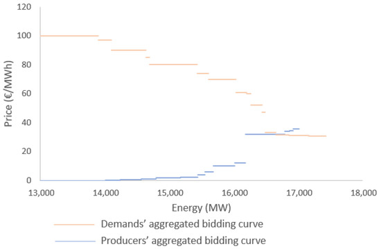
Figure 3.
Aggregated market curves for a given hour. The resulting function is not continuous.
To address this issue, the curve fitting will be made over the midpoint of each block:
Consider any offer block i in the market curve as:
where V is the volume offered and p its price at time period h. The coordinates of the block in the curve are:
where:
The interpolation points are then
Another point to bear in mind is that these points are not evenly spaced, and since curve fitting is performed with the least squares method, the concentration of points in a given part of the curve can affect the results. A simple way to avoid the problem is to linearly interpolate the points in (8) and then take a new set of evenly spaced points from the interpolation results.
Since there are two distinct market curves, supply and demand, we have in fact two sets of coordinate pairs and will need two functions and to correctly simulate the market, which implies two distinct parameter vector and , bringing some complexity to the system under study. However, as a turnaround to this complexity and recalling the advantages of the curves—price sensitivity to demand volume changes, confidence intervals over price forecasts and portfolio optimization—we can achieve the same results looking at the difference:
where is the demand curve, and is the supply curve.
This leads to only one single function and only one set of parameters. Let us call this function the “price sensitivity curve”, since it is a direct measure of the price changes over volume. The electricity price can be found in the root of this function, more precisely:
On a practical point of view, since the price is the image of the supply (or demand) curve on the root , we can simplify the electricity price calculation by taking its inverse:
This way the market clearing price will be the root of .
The curve fitting was evaluated using different functions: polynomials of different orders, sigmoid functions and stepwise linear functions. The purpose of the method is to have the curve shape around the MCP, meaning that the curve fitting has to be weighted to points near the root of . To understand how the curve behaves near its root, we calculated the MCP as the root of the fitted function and calculated the error to the real price observed. The best fit was found using a sixth degree polynomial , where the parameters are estimated using the weighted least squares method.
The parameters can be seen as the representation of the market curve . Our main objective is to find patterns and relationships between these variables so that we can, with a given set of exogenous variables, find the respective market curve.
4.2. Parameter Analysis
By observing Figure 4, where every parameter is plotted, it is possible to perceive their time series behaviour as well as some level of seasonality.
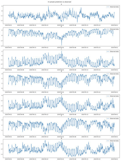
Figure 4.
From top to bottom, the observed data for all 7 standardized parameters a, b, c, d, e, f and g.
To include seasonality in the model, we first studied the periodicity of the data series by computing its power spectrum and analyzing the periodogram (Figure 5). For low frequencies, the spectrum shows a peak at frequency , representing a cycle of 168 h, i.e., weekly seasonality. For low frequencies, the highest peak is shown at frequency , representing a cycle of 24 h, i.e., daily seasonality. In both cases, the spectrum shows lower peaks at frequencies that are multiples of the ones already identified.
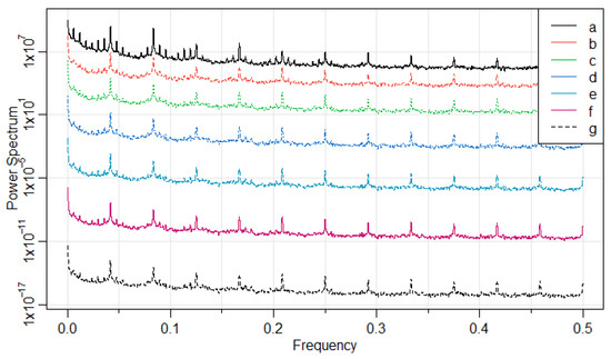
Figure 5.
Calculated power spectrum for the market curve parameters.
4.3. Curve Forecast Model
The model proposed consists of a combination of a vector autoregressive (VAR) model with a seasonal harmonic component of periods 24 and 168 and dynamic exogenous variables. This model captures the autoregressive behavior of the time series as well as the autocorrelations between the parameters. The harmonic component helps to correctly model the seasonality of the parameters, and since electricity prices are highly dependent on external variables such as electricity demand or wind and solar production, which are time series per se, the dynamic external variables are essential to capture the dynamics of the market curves.
The autoregressive models were lightly described in Section 3. Recalling the notation, we can write our model:
where are the m endogenous market curve parameters, B is the backward shift operator , is the notation for , are coefficient matrixes for the autoregressive terms, are l coefficient matrixes for the n dynamic exogenous variables for each lag l, and the coefficient vectors for the harmonics, are the number of harmonic terms for each period and a white noise process with mean 0 and covariance matrix .
The parameters can be estimated with an ordinary least squares method and the hyperparameters p, l and K can be obtained by performing a search on the hyperparameter space.
Summarizing, all the process consists of: (1) supply and demand curve interpolation; (2) price sensitivity estimation through the difference of the demand and the supply interpolated curves and its inversion to obtain the market curve in the study; (3) market-curve fitting to known parametric function; (4) parameter forecast with the model in (12); and (5) electricity price forecasting by finding the root of the forecast curve (Figure 6).
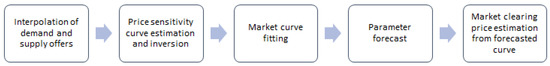
Figure 6.
Flowchart of the proposed method for electricity price estimation with market curves forecasting.
5. Empirical Results
5.1. Market Data
For the construction and evaluation of this model, we used market curves data from 2017 to 2020 from the Iberian Market OMIE. These data include all the offers (energy, price) from market agents for each hour of the period.
We also include in the analysis different market data available, such as wind production forecasts, solar production forecasts, load forecasts, availability forecasts for different technologies, interconnection capacity and forecasts and French and German market data. These data will be used as exogenous variables in the model and will help explain the curve shape for the future.
5.2. Forecasting Evaluation
Most literature agrees on the forecasting evaluation methods and metrics and sometimes even provide different metrics for their forecasts. Measuring point forecasting accuracy is based on absolute errors , where is the actual and is the predicted price for the period h. Obviously, the accuracy will increase with lower . For hourly forecasts, it is quite commons to see a Mean Average Error (MAE) as the mean of the absolute errors over the forecast period T:
Since electricity prices can change significantly from market to market, absolute errors are quite hard to compare between different datasets. Many authors use measures based on absolute percentage errors: . By far the most popular is the Mean Average Percentage Error (MAPE), which is computed as the mean of absolute percentage errors over T:
The MAPE measure is suitable for markets where prices are significantly higher than zero, but it can be misleading when applied to most electricity prices. In particular, when electricity prices are close to zero, MAPE values become very large, regardless of the actual absolute errors. On the other hand, when electricity prices spike, the resulting MAPE values are small, irrespective of the absolute differences. In a balance sheet impact point of view, this is inaccurate since a badly forecast price spike might have a much bigger financial impact than a poorly forecast price close to zero.
The most common approach to tackle the comparison issues between different models and different price scales is to normalize the absolute error by the average price obtained in the evaluation interval T. This yields the Weighted Mean Average Error (WMAE):
where is the mean price in the time interval T.
For this reason, the metric used for the model evaluation are the MAE and WMAE.
5.3. Model Hyperparameter Selection
Since the basis of the model proposed is a VAR model for forecasting the market curves parameters, it is important to guarantee that all of the variables are stationary. To check the stationarity of the time series, we used the Augmented Dickey–Fuller (ADF) test, which tests the null hypothesis that a unit root is present in the sample. The p-value obtained for all the parameters was , rejecting the null hypothesis and demonstrating that the time series are indeed stationary.
The hyperparameters of the model, the number of lags p for the VAR model, the number of lags l for the exogenous variables and the max iteration K for Fourier Series were estimated by performing a grid search. We ran a range of values for each parameter: p between 1 and 168, l between 1 and 24 and K between 1 and 12 and evaluated the model performance in three distinct ways: computing information criterion AIC, BIC e HQIC, calculating the MAE of each parameter and calculating the MAE of the resulting electricity price. Since the main target is to predict the market curves, the combination of parameters with a lower combined MAE for the seven parameters was chosen.
The criteria were evaluated for one year of in-sample data, and the errors for the parameters and price were calculated for 1 month of out-sample predictions. The results can be summarized in:
- The AIC shows a descending trend until and an ascending trend for higher values. This shows that for this criterion the model should be complex enough, having a high number of lags in the autoregressive term;
- On the other hand, the BIC and HQIC seem to be lower with lower parameters (low p, l and K) and start rising rapidly, suggesting a more simple model. However, the out-sample residuals of parameters and price for the models with lower BIC/HQIC, are higher than what is expected in the industry sector;
- For the parameters error, the higher order parameters MAE was lower with , but for the lower order parameters, the lowest MAE was found for . Since we are in the presence of seven distinct parameters, it is not possible to find a scenario where all the parameters MAE are lower. However, when comparing the two hypothesis just mentioned, the average of the MAE is lower for ;
- The price MAE is lower when or , showing some relationship with the parameters MAE;
- For every measure, the best models for the remaining hyperparameter were found for and .
After observing these results, the model chosen consisted of the hyperparameters , and . We ran the model for 2019 and 2020 and calculated the out-sample predictions for each hour and then compared to some of the best models used in the industry, both statistical and machine learning.
5.4. Model Benchmark
The model was benchmarked against other models used in the sector, both statistical and machine learning, and the results obtained can be seen in Table 1.

Table 1.
Model results and benchmark against industry sector models.
The statistical models are dynamic regression models with different combinations of the exogenous variables already discussed in this work and used in the market curves VAR model. The ELM models have a 500 sample random runs, and their average is considered as the final forecast. They use different exogenous variables between them but the same hyperparameters. The XGBOOST have a significant difference to the other models; they use the results from the other models, statistical and machine learning, as inputs, working as an ensemble algorithm for the other forecasts, being able to fine tune them.
These models forecast the electricity hourly price itself; so, to benchmark the model proposed in this thesis, the metric used for comparison is the electricity price MAE and WMAE although the model actually forecast the market curves for each hour of the day ahead.
It is shown that the market curve model outperforms the non-ensemble models, i.e., the different statistical models already employed in the sector and the ELM models, falling just short of the XGBOOST models. However, as already stated, the XGBOOST models work as an ensemble for the forecasts obtained with the other methods, using them as an input. All the known market variables exogenous to the other models work are also used in XGBOOST as dependent variables.
Since the proposed model outperforms the pure electricity price forecasting ones—statistical and ELM—it is reasonable to conclude that it captures some information that the others cannot find, leading to lower errors. On the other hand, the comparison with XGBOOST is proof of what is seen in the literature: ensemble models have better performance than individual forecasting model, being able to capture the advantages of each model while evading the disadvantages.
Since this is an ensemble model, it is possible to include the new market curve results in the pool of forecasts already used. By doing this, the MAE of the XGBOOST can decrease to €2.2/MWh as seen in Table 2.
Table 2.
Using the market curve forecasts in the XGBOOST clearly improves the forecasts.
This means that, not only does the market curve model outperform all the other pure price forecasting models, but it also adds relevant information to the ensemble, significantly improving its results. This shows the the proposed model is useful for capturing market dynamics that the other models cannot, dynamics that are only obtainable with the ask/bid offers information.
Moreover, the model has shown a good adaptability when there are significant price changes, being able to capture regime changes better than any other model. By calculating the MAE of the models in the days, where the average daily price changes by more than three standard deviations, we can see a lower error than in the XGBOOST that can be improved even further by including the market curve price forecasts, as shown in Table 3. The market curves can actually capture the nonlinearity of the electricity prices, indicating that most of it might come from the bid and ask offer in the market.
Table 3.
MAE of the models when evaluated on the days where the average daily price changes by more than 3 standard deviations.
6. Discussion and Conclusions
The challenge of predicting electricity prices in a complex market with high volatility makes EPF a very interesting field. In the industry sector point of view, EPF is a must-have for energy management, since it is impossible to correctly dispatch energy or manage risk without accurate electricity price predictions.
In the actual context, accurate predictions become more than just a management tool, they are a differentiating factor from the competition. Researching and investing in new EPF models is needed to remain competitive. This thesis presents not only a new method for EPF, but a new framework for researchers to work with. Looking at the market curves instead of the electricity price has proven more efficient than the traditional point forecasts for electricity prices.
A new market curve model was developed for forecasting electricity prices. This new approach is not only useful for electricity price forecasting, but also brings clear advantages for risk management in the industry sector. There is no other model that uses this approach to electricity price forecasting, as models and methods proposed often disregard the market curves structures that are behind the market clearing price.
The electricity price forecasts made by the market curve model outperformed traditional statistical models and some machine learning models and also showed a capacity to adapt to extreme price changes. Regime changes in time series are always hard to forecast without a complete knowledge of the underlying processes. In the electricity price forecast, the underlying process are the market curves. Incorporating them into the forecasts increases the adaptability of the model in scenarios where there are abrupt changes to the price. In addition, it gives an actual forecast for the market curves, in particular to the price sensitivity curve, given by the difference between the demand and the supply. This is an extra measure of this model and thus is not comparable to the other models in the industry sector.
Although the model proposed in this work is classic in the sense of the techniques used—vector autoregression with exogenous variables and an harmonic factor for seasonality—it is able to obtain better results than the models that are actually used by the industry sector in its everyday operations. This shows that the method of using and forecasting the market curves/offers, which is a novel method built for this model, is essential for EPF and must be studied.
This approach is innovative in the sense that the models described in the literature do not incorporate the information about the bids/asks in their price forecasts, and this is, most probably, the first model with a practical application to be designed with the market curves.
There are two important points to take from this work: First, modelling, identifying and forecasting market curves is complex, and there is still much room to improve. The second point is that incorporating this knowledge in electricity price forecasting gives better results than traditional models and gives additional information that is not usually captured by the other models.
This work suggested a parameterization of the curves by fitting them to a known easier to work function and then analyzing these parameters. However, more complex methods with a higher number of parameters can be used and will probably lead to better overall forecasts. Comparison and similarity analysis between curves can also be performed to add extra information to a market curve forecast model. Other forecasting techniques can also be applied, such as applying feature selection techniques to the exogenous variables, the state-of-art statistical models, or machine learning techniques for curve forecasting.
Author Contributions
Conceptualization, M.P., M.F. and R.C.; methodology, M.P. and M.F.; formal analysis, M.P.; writing—original draft preparation, M.P.; writing—review and editing, M.P.; visualization, M.P.; All authors have read and agreed to the published version of the manuscript.
Funding
This research received no external funding.
Institutional Review Board Statement
Not applicable.
Informed Consent Statement
Not applicable.
Data Availability Statement
All aggregated curve and market data can be found in https://www.omie.es/es/file-access-list (accessed on 1 May 2021).
Conflicts of Interest
The authors declare no conflict of interest.
References
- Bunn, D. Forecasting loads and prices in competitive power markets. Proc. IEEE 2000, 88, 163–169. [Google Scholar] [CrossRef]
- Bastian, J.; Zhu, J.; Banunarayanan, V.; Mukerji, R. Forecasting energy prices in a competitive market. IEEE Comput. Appl. Power 1999, 12, 40–45. [Google Scholar] [CrossRef]
- Contreras, J.; Espinola, R.; Nogales, F.J.; Conejo, A.J. Forecasting electricity prices for a day-ahead pool-based electric energy market. Int. J. Forecast. 2005, 21, 435–462. [Google Scholar]
- Ferreira, L.A.F.M.; Andersson, T.; Imparato, C.F.; Miller, T.E.; Pang, C.K.; Svoboda, A.; Vojdani, A.F. Short-term resource scheduling in multi-area hydrothermal power systems. Int. J. Electr. Power Energy Syst. 1989, 11, 200–212. [Google Scholar] [CrossRef]
- Catalao, J.P.D.S.; Mariano, S.J.P.S.; Mendes, V.M.F.; Ferreira, L.A.F.M. Parameterisation effect on the behaviour of a head-dependent hydro chain using a nonlinear model. Electr. Power Syst. Res. 2006, 76, 404–412. [Google Scholar] [CrossRef][Green Version]
- Mendes, V.M.F.; Mariano, S.J.P.S.; Catalão, J.P.S.; Ferreira, L.A.F.M. Emission constraints on short-term schedule of thermal units. In Proceedings of the 39th International Universities Power Engineering Conference, Bristol, UK, 6–8 September 2004; pp. 1068–1072. [Google Scholar]
- Fosso, O.B.; Gjelsvik, A.; Haugstad, A.; Mo, B.; Wangensteen, I. Generation scheduling in a deregulated system. The Norwegian case. IEEE Trans. Power Syst. 1999, 14, 75–80. [Google Scholar] [CrossRef]
- Stoft, S. Power System Economics: Designing Markets for Electricity; Wiley-IEEE Press: Piscataway, NJ, USA, 2002. [Google Scholar]
- Chao, H.; Hillard, H. Designing Competitive Electricity Markets; Springer: Boston, MA, USA, 1998. [Google Scholar]
- Mousavi, F.; Nazari-Heris, M.; Mohammadi-Ivatloo, B.; Asadi, S. Energy market fundamentals and overview. In Energy Storage in Energy Markets; Academic Press: Cambridge, MA, USA, 2021; pp. 1–21. [Google Scholar]
- Huisman, R.; Huurman, C.; Mahieu, R. Hourly electricity prices in day-ahead markets. Energy Econ. 2007, 29, 240–248. [Google Scholar] [CrossRef]
- Uniejewski, B.; Nowotarski, J.; Weron, R. Automated variable selection and shrinkage for day-ahead electricity price forecasting. Energies 2016, 9, 621. [Google Scholar] [CrossRef]
- Ziel, F.; Weron, R. Day-ahead electricity price forecasting with high-dimensional structures: Univariate vs. multivariate modeling frameworks. Energy Econ. 2018, 70, 396–420. [Google Scholar] [CrossRef]
- Uniejewski, B.; Weron, R. Efficient forecasting of electricity spot prices with expert and lasso models. Energies 2018, 11, 2039. [Google Scholar] [CrossRef]
- Lago, J.; De Ridder, F.; De Schutter, B. Forecasting spot electricity prices: Deep learning approaches and empirical comparison of traditional algorithms. App. Energy 2018, 221, 386–405. [Google Scholar] [CrossRef]
- Ziel, F.; Steinert, R.; Husmann, S. Forecasting day ahead electricity spot prices: The impact of the EXAA to other European electricity markets. Energy Econ. 2015, 51, 430–444. [Google Scholar] [CrossRef]
- Ziel, F. Forecasting electricity spot prices using lasso: On capturing the autoregressive intraday structure. IEEE Trans. Power Syst. 2016, 31, 4977–4987. [Google Scholar] [CrossRef]
- Jahangir, H.; Tayarani, H.; Baghali, S.; Ahmadian, A.; Elkamel, A.; Golkar, M.A.; Castilla, M. A Novel Electricity Price Forecasting Approach Based on Dimension Reduction Strategy and Rough Artificial Neural Networks. IEEE Trans. Ind. Inform. 2020, 16, 2369–2381. [Google Scholar] [CrossRef]
- Hubicka, K.; Marcjasz, G.; Weron, R. A note on averaging day-ahead electricity price forecasts across calibration windows. IEEE Trans. Sustain. Energy 2019, 10, 321–323. [Google Scholar] [CrossRef]
- Marcjasz, G.; Seran, T.; Weron, R. Selection of calibration windows for day-ahead electricity price forecasting. Energies 2018, 11, 2364. [Google Scholar] [CrossRef]
- Jónsson, T.; Pinson, P.; Nielsen, H.A.; Madsen, H.; Nielsen, T.S. Forecasting electricity spot prices accounting for wind power predictions. IEEE Trans. Sustain. Energy 2013, 4, 210–218. [Google Scholar] [CrossRef]
- Garcia-Martos, C.; Rodriguez, J.; Sanchez, M.J. Mixed models for short-run forecasting of electricity prices: Application for the Spanish market. IEEE Trans. Power Syst. 2007, 22, 544–551. [Google Scholar] [CrossRef]
- Conejo, A.; Plazas, M.; Espínola, R.; Molina, A. Day-ahead electricity price forecasting using the wavelet transform and ARIMA models. IEEE Trans. Power Syst. 2005, 20, 1035–1042. [Google Scholar] [CrossRef]
- Shafie-Khah, M.; Moghaddam, M.; Sheikh-El-Eslami, M. Price forecasting of day-ahead electricity markets using a hybrid forecast method. Energy Convers. Manag. 2011, 52, 2165–2169. [Google Scholar] [CrossRef]
- Lagarto, J.; De Sousa, J.; Martins, A.; Ferrão, P. Price forecasting in the day-ahead Iberian electricity market using a conjectural variations ARIMA model. In Proceedings of the 2012 9th International Conference on the European Energy Market, Florence, Italy, 10–12 May 2012. [Google Scholar]
- Johnsen, T. Demand, generation and price in the Norwegian market for electric power. Energy Econ. 2001, 23, 227–251. [Google Scholar] [CrossRef]
- Marcos, R.A.; Bello, A.; Reneses, J. Electricity price forecasting in the short term hybridising fundamental and econometric modelling. Electr. Power Syst. Res. 2019, 167, 240–251. [Google Scholar] [CrossRef]
- Barlow, M. A diffusion model for electricity prices. Math. Financ. 2002, 12, 287–298. [Google Scholar] [CrossRef]
- Kanamura, T.; Ohashi, K. A structural model for electricity prices with spikes: Measurement of spike risk and optimal policies for hydropower plant operation. Energy Econ. 2007, 29, 1010–1032. [Google Scholar] [CrossRef]
- Gonzalez, A.; San Roque, A.; Garcia-Gonzalez, J. Modeling and forecasting electricity prices with input/output hidden Markov models. IEEE Trans. Power Syst. 2005, 20, 13–24. [Google Scholar]
- Mandal, P.; Senjyu, T.; Funabashi, T. Neural networks approach to forecast several hour ahead electricity prices and loads in deregulated market. Energy Convers. Manag. 2006, 47, 2128–2142. [Google Scholar] [CrossRef]
- Amjady, N. Day-ahead price forecasting of electricity markets by a new fuzzy neural network. IEEE Trans. Power Syst. 2006, 21, 887–996. [Google Scholar] [CrossRef]
- Hu, Z.; Yang, L.; Wang, Z.; Gan, D.; Sun, W.; Wang, K. A game-theoretic model for electricity markets with tight capacity constraints. Int. J. Electr. Power 2008, 30, 207–215. [Google Scholar] [CrossRef]
- Rodriguez, C.; Anders, G. Energy price forecasting in the Ontario competitive power system market. EEE Trans. Power Syst. 2004, 19, 366–374. [Google Scholar] [CrossRef]
- Areekul, P.; Senju, T.; Toyama, H.; Chakraborty, S.; Yona, A.; Urasaki, N.; Mandal, P.; Saber, A.Y. A new method for next-day price forecasting for PJM electricity market. Int. J. Electr. Power 2010, 11, 2. [Google Scholar] [CrossRef]
- Guo, J.; Luh, P. Improving market clearing price prediction by using a committee machine of neural networks. IEEE Trans. Power Syst. 2004, 19, 1867–1876. [Google Scholar] [CrossRef]
- Pao, H. A Neural Network Approach to m-Daily-Ahead Electricity Price Prediction; Lecture Notes in Computer Science; Springer: Berlin/Heidelberg, Germnay, 2006; pp. 1284–1289. [Google Scholar]
- Yamin, H.; Shahidehpour, S.; Li, Z. Adaptive short-term electricity price forecasting using artificial neural networks in the restructured power markets. Int. J. Electr. Power 2004, 26, 571–581. [Google Scholar] [CrossRef]
- Aggarwal, S.; Saini, L.; Kumar, A. Electricity price forecasting in deregulated markets: A review and evaluation. Int. J. Electr. Power 2009, 31, 13–22. [Google Scholar] [CrossRef]
- Catalão, J.; Mariano, S.; Mendes, V.; Ferreira, L. Short-term electricity prices forecasting in a competitive market: A neural network approach. Electr. Power Syst. Res. 2007, 77, 1297–1304. [Google Scholar] [CrossRef]
- Pindoriya, N.; Singh, S.; Singh, S. An adaptive wavelet neural network-based energy price forecasting in electricity markets. IEEE Trans. Power Syst. 2008, 23, 1423–1432. [Google Scholar] [CrossRef]
- Amjady, N.; Hemmati, M. Day-ahead price forecasting of electricity markets by a hybrid intelligent system. Int. J. Electr. Power 2009, 19, 89–102. [Google Scholar] [CrossRef]
- Chen, Y.; Wang, Y.; Ma, J.; Jin, Q. BRIM: An Accurate Electricity Spot Price Prediction Scheme-Based Bidirectional Recurrent Neural Network and Integrated. Energies 2019, 12, 2241. [Google Scholar] [CrossRef]
- Ugurlu, U.; Oksuz, I.; Tas, O. Electricity Price Forecasting Using Recurrent Neural Networks. Energies 2018, 11, 1255. [Google Scholar] [CrossRef]
- Sansom, D.; Downs, T.; Saha, T. Evaluation of support vector machine based forecasting tool in electricity price forecasting for Australian national electricity market participants. J. Electr. Electron. Eng. Aust. 2002, 22, 227–233. [Google Scholar]
- Che, J.; Wang, J. Short-term electricity prices forecasting based on support vector regression and autoregressive integrated moving average modeling. Energy Convers. Manag. 2010, 51, 1911–1917. [Google Scholar] [CrossRef]
- Hong, Y.; Hsiao, C. Locational marginal price forecasting in deregulated electricity markets using artificial intelligence. IEE Proc. Gener. Transm. Distrib. 2002, 149, 621–626. [Google Scholar] [CrossRef]
- Vahidinasab, V.; Jadid, S.; Kazemi, A. Day-ahead price forecasting in restructured power systems using artificial neural networks. Electr. Power Syst. Res. 2008, 78, 1332–1342. [Google Scholar] [CrossRef]
- Wang, L.; Zhang, Z.; Chen, J. Short-term electricity price forecasting with stacked denoising autoencoders. IEEE Trans. Power Syst. 2016, 32, 2673–2681. [Google Scholar] [CrossRef]
- Yang, Z.; Ce, L.; Lian, L. Electricity price forecasting by a hybrid model, combining wavelet transform, ARMA and kernel based extreme learning machine methods. App. Energy 2017, 190, 291–305. [Google Scholar] [CrossRef]
- Zhang, J.; Tan, Z.; Li, C. A novel hybrid forecasting method using GRNN combined with wavelet transform and a GARCH model. Energy Source Part B 2015, 10, 418–426. [Google Scholar] [CrossRef]
- Hong, Y.Y.; Liu, C.Y.; Chen, S.J.; Huang, W.C.; Yu, T.H. Short-term LMP forecasting using an artificial neural network incorporating empirical mode decomposition. Int. Trans Electr. Energy Syst. 2014, 25, 1952–1964. [Google Scholar] [CrossRef]
- Zhang, J.L.; Zhang, Y.J.; Li, D.Z.; Tan, Z.F.; Ji, J.F. Forecasting day-ahead electricity prices using a new integrated model. Int. J. Electr. Power Energy Syst. 2019, 105, 541–548. [Google Scholar] [CrossRef]
- Varshney, H.; Sharma, A.; Kumar, R. A hybrid approach to price forecasting incorporating exogenous variables for a day ahead electricity market. In Proceedings of the 2016 IEEE International Conference on Power Electronics, Intelligent Control and Energy Systems, Delhi, India, 4–6 July 2016. [Google Scholar]
- Xiao, L.; Shao, W.; Yu, M.; Ma, J.; Jin, C. Research and application of a hybrid wavelet neural network model with the improved cuckoo search algorithm for electrical power system forecasting. App. Energy 2017, 198, 203–222. [Google Scholar] [CrossRef]
- Khajeh, M.; Maleki, A.; Rosen, M.; Ahmadi, M. Electricity price forecasting using neural networks with an improved iterative training algorithm. Int. J. Ambient. Energy 2017, 39, 147–158. [Google Scholar] [CrossRef]
- Bisoi, R.; Dash, P.; Das, P. Short-term electricity price forecasting and classication in smart grids using optimized multikernel extreme learning machine. Neural Comput. Appl. 2018, 32, 1457–1480. [Google Scholar] [CrossRef]
- Kim, M. Short-term price forecasting of nordic power market by combination Levenberg-Marquardt and cuckoo search algorithms. IET Gener. Transm. Distrib. 2015, 9, 1553–1563. [Google Scholar] [CrossRef]
- Gao, W.; Sarlak, V.; Parsaei, M.; Ferdosi, M. Combination of fuzzy based on a meta-heuristic algorithm to predict electricity price in an electricity markets. Chem. Eng. Res. Des. 2018, 131, 333–345. [Google Scholar] [CrossRef]
- Abedinia, O.; Amjady, N.; Shae-khah, M.; Catalão, J. Electricity price forecast using combinatorial neural network trained by a new stochastic search method. Energy Convers. Manag. 2015, 105, 642–654. [Google Scholar] [CrossRef]
- Itaba, S.; Mori, H. An electricity price forecasting model with fuzzy clustering preconditioned ANN. Electr. Eng. Jpn. 2018, 204, 10–20. [Google Scholar] [CrossRef]
- Nazar, M.S.; Fard, A.E.; Heidari, A.; Shafie-khah, M.; Catalao, J.P. Hybrid model using three-stage algorithm for simultaneous load and price forecasting. Electr. Power Syst. Res. 2018, 165, 214–228. [Google Scholar] [CrossRef]
- Ghofrani, M.; Azimi, R.; Najafabadi, F.; Myers, N. A new day-ahead hourly electricity price forecasting framework. In Proceedings of the 2017 North American Power Symposium, Morgantown, WV, USA, 17–19 September 2017; pp. 1–6. [Google Scholar]
- Pourdaryaei, A.; Mokhlis, H.; Illias, H. Short-term electricity price forecasting via hybrid backtracking search algorithm and ANFIS approach. IEEE Access 2019, 7, 77674–77691. [Google Scholar] [CrossRef]
- Itaba, S.; Mori, H. A fuzzy-preconditioned GRBFN model for electricity price forecasting. Procedia Comput. Sci. 2017, 114, 441–448. [Google Scholar]
- Gobu, B.; Jaikumar, S.; Arulmozhi, N.; Kanimozhi, P. Two-stage machine learning framework for simultaneous forecasting of price-load in the smart grid. In Proceedings of the 2018 IEEE International Conference on Machine Learning and Applications, Orlando, FL, USA, 17–20 December 2018; pp. 1081–1086. [Google Scholar]
- Olamaee, J.; Mohammadi, M.; Noruzi, A.; Hosseini, S. Day-ahead price forecasting based on hybrid prediction model. Complexity 2016, 21, 156–164. [Google Scholar] [CrossRef]
- Bordignon, S.; Bunn, D.; Lisi, F.; Nan, F. Combining day-ahead forecasts for British electricity prices. Energy Econ. 2013, 35, 88–103. [Google Scholar] [CrossRef]
- Maciejowska, K. Fundamental and speculative shocks, what drives electricity prices? In Proceedings of the 11th International Conference on the European Energy Market (EEM14), Krakow, Poland, 28–30 May 2014. [Google Scholar]
- Nowotarski, J.; Weron, R. Computing electricity spot price prediction intervals using quantile regression and forecast averaging. Comput. Stat. 2015, 30, 791–803. [Google Scholar] [CrossRef]
- Raviv, E.; Bouwman, K.; van Dijk, D. Forecasting day-ahead electricity prices: Utilizing hourly prices. Tinbergen Inst. Discuss. Pap. 2013, 30, 1030–1081. [Google Scholar] [CrossRef][Green Version]


Publisher’s Note: MDPI stays neutral with regard to jurisdictional claims in published maps and institutional affiliations. |
© 2022 by the authors. Licensee MDPI, Basel, Switzerland. This article is an open access article distributed under the terms and conditions of the Creative Commons Attribution (CC BY) license (https://creativecommons.org/licenses/by/4.0/).