Supervisory Event-Triggered Control of Uncertain Process Networks: Balancing Stability and Performance ^†

Abstract

This work presents a methodological framework for the design of a resource-aware supervisory control system for process networks with model uncertainty and communication resource constraints. The developed framework aims to balance the objective of closed-loop stabilization of the overall network with that of meeting the local performance requirements of the component subsystems while keeping the rate of data transfer between the local control systems to a minimum. First, a quasi-decentralized networked control structure, with a set of local model-based controllers communicating with one another over a shared communication medium at discrete times, is designed. A Lyapunov stability analysis of the closed-loop system is then carried out, and the results are used to derive appropriate bounds on the local model state estimation errors as well as the dissipation rates of the local control Lyapunov functions. These bounds are used as stability and performance thresholds to trigger communication between the local control systems and a higher-level supervisor that coordinates the transfer of state measurements between the distributed control systems. A breach of the local stability and performance thresholds generates alarm signals which are transmitted to the supervisor to determine which subsystems should communicate with one another. The supervisor employs a composite Lyapunov function to assess the impact of the local threshold breaches on the stability of the overall closed-loop system. The supervisory communication logic takes account of the evolution of the local and composite Lyapunov functions in order to balance the stability and local performance requirements. Finally, the developed framework is demonstrated using a representative chemical process network and compared with other unsupervised event-based control approaches. It is shown that the supervisory event-based control approach leads to a more judicious utilization of network resources that helps improve closed-loop process performance in the presence of unexpected disturbances and input rate constraints.

1. Introduction

Modern chemical processing plants comprise of geographically distributed processing units that are typically arranged in a complex network. The networked structure of these systems is often the result of the physical interconnections between processing units through material and energy flows and recycling. These interconnections, which are increasingly relied upon to address safety, economic and environmental concerns in process operations, can lead to difficulties in the design and operation of plant-wide control and supervision systems as the resulting large-scale system may have complex dynamics. The theoretical and practical challenges associated with this problem have motivated an extensive and growing body of research work and have led to the development of numerous methodologies for the control and monitoring of chemical process networks. Examples of contributions in this area include methods for the design of centralized and decentralized control systems (e.g., [1,2,3,4]), approaches for the design of multi-scale control systems (e.g., [5,6]), passivity-based control designs (e.g., [7,8,9]), multi-agent based control methodologies (e.g., [10,11]), and optimization-based cooperative and distributed predictive control methods (e.g., [12,13,14]).

In addition to handling the complex dynamics induced by physical interactions, the management of information transfer and communication between the constituent subsystems is an increasingly important consideration in the design of supervisory control systems for process networks. The last two decades have witnessed growing calls from the industrial and academic communities for the adoption of a new paradigm for process operations, referred to as the smart plant paradigm [15,16]. This paradigm calls for tighter coupling between the decision-making processes across the different plant layers through real-time information exchange. A key enabling element of this paradigm is the integration of real-time shared communication networks (such as wireless sensor and actuator networks) in process monitoring and control systems. The realization that the deployment of advanced communication technologies in plant-wide control systems not only leads to substantial economic savings but also enhances the operational flexibility of the process provides a strong incentive for the adoption of smart plant operations. This realization has been an important factor in driving the shift from hard-wired dedicated links to networked control architectures in industrial control systems. With the advent and adoption of networked control technologies, the component subsystems in a plant become interconnected not only through material and energy flows, which give rise to the process network, but also through information flow, which gives rise to the control network.

Notwithstanding the appealing operational and economic opportunities created by networked control systems, it is well understood that the integration of shared communication networks in general (and wireless networks in particular) in control systems poses fundamental challenges. These challenges, which often stem from the inherent limitations on the computational, processing and communication resources of the shared communication media, have motivated a plethora of research studies in this area. Comprehensive reviews of recent advances and challenges in the analysis, synthesis and security of networked control systems can be found in survey papers [17,18,19,20,21,22,23]. On the one hand, maximizing process performance generally requires increased levels of communication between the individual subsystems. On the other hand, conserving network resources, which may be necessary to prolong the network service life and minimize data losses, favors limiting unnecessary information exchange over the network. Meeting this challenge ultimately requires carefully balancing the stability and performance needs of the overall system against the required levels of information exchange and network resource utilization.

An early effort to address the network resource utilization problem for large-scale process networks was pursued in [24]. This effort led to the development of a model-based quasi-decentralized control strategy that achieves closed-loop stability with minimal periodic communication between the constituent subsystems. The main idea was to embed a set of predictive models within each local control system to estimate the plant states when communication over the plant-wide network was suspended. The state estimates were used together with the locally available state measurements to generate the local control action during periods of communication suspension. To provide the necessary corrective feedback action, communication was restored at discrete times to allow the transmission of state measurements which were used to update the states of the embedded models. A key outcome of that effort was a rigorous characterization of the relationship between the minimum allowable communication rate, the controller design parameters and the plant–model mismatch.

In a subsequent study [25], an adaptive event-based communication logic was introduced to manage the information exchange between the local control systems in the quasi-decentralized control structure. The main idea of this strategy was to suspend communication for as long as the closed-loop system remained stable, and to allow communication only when any of the individual subsystems was on the verge of instability. To realize this strategy, a stability-based state-dependent alarm threshold was developed for each subsystem with the aid of an appropriate control Lyapunov function, and used to trigger communication between the local control systems. Each subsystem monitored its local state evolution and prompted the other subsystems to transmit their state measurements to update the corresponding models only when the prescribed alarm threshold was breached. Compared with the time-triggered periodic communication approach, this feedback-based communication strategy generally leads to greater operational flexibility and improved closed-loop performance when responding to unexpected disturbances. However, it also has the potential to increase the network load, which could exacerbate problems such as data losses and communication delays when a large number of subsystems attempt to access the network simultaneously.

To alleviate the potential problem of increased network load, a decentralized communication strategy was developed in [26,27,28]. In this approach, an additional model of the local subsystem dynamics is included and used to monitor the evolution of the model state estimation error shared in the other plant subsystems. A composite Lyapunov function for the overall plant is used to obtain transmission thresholds that trigger the broadcast of state information over the network. Specifically, a local model state estimation error of a certain subsystem exceeding the local threshold would prompt a broadcast of the local state measurements to the rest of the plant to maintain closed-loop stability. This approach can be considered proactive in the sense that a given subsystem broadcasts its information to the rest of the plant based on a breach of the local transmission threshold, regardless of the actual state or needs of the other subsystems in the plant. This is in contrast to the adaptive request-based nature of the prior approach in [25] where, upon breach of the local alarm threshold, a given subsystem requests measurement updates from the other subsystems.

The broadcast-based nature of the decentralized communication strategy has the advantage of avoiding the necessity for all subsystems to access the network at the same time. However, as the local transmission thresholds are designed on the basis of a composite Lyapunov function, the focus of that approach is limited to enforcing the closed-loop stability of the plant, without accounting for the performance of the individual subsystems. This can lead to significant performance degradation in some situations. For example, in the event that a transient local disturbance results in a transient growth of the local Lyapunov function (thus deteriorating the local performance) without causing the composite Lyapunov function to grow, no communication (and no model updates) would be triggered by the decentralized communication strategy since the stability-based transmission thresholds are not breached. The lack of communication between the local control systems in this case makes it impossible to rectify the resulting performance deterioration. Therefore, the potential benefits of reducing network utilization could be lost, or at least limited, by the resulting degradation in local process performance.

To address the potential limitations of fully decentralized communication strategies, a supervisory event-triggered control approach that aims to balance the overall closed-loop stability and local performance objectives was introduced in [29]. The key idea was to design a hierarchical control structure in which a family of lower-level model-based controllers exchange state measurements at discrete times, and a higher-level supervisor coordinates communication between the local controllers on the basis of an event-triggered communication logic. The local controllers transmit alarm signals to the supervisor in the event that certain thresholds on either the local model state estimation error or the local Lyapuonv function are breached. The supervisor tracks the alarm signals and decides accordingly which subsystems should be allowed to transmit their data over the plant-wide network.

Building on our prior work, the objectives of the current work are to establish the theoretical foundation for the supervisory control approach introduced in [29] and to evaluate its capabilities in reducing network utilization rates in the presence of practical implementation challenges. On the theoretical front, the current study provides a rigorous characterization of the underlying closed-loop stability properties which serve as the foundation for the development and implementation of the supervisory control logic. Specifically, a Lyapunov stability analysis of the overall closed-loop system is carried out, and the results are used to obtain explicit bounds on the local model state estimation errors and the dissipation rates of the local control Lyapunov functions. These bounds are used as stability and performance thresholds to trigger communication between the local control systems on the one hand, and the higher-level supervisor on the other. The supervisory control logic is designed to address both the stability and performance requirements as it takes into account the behavior of both the local and composite control Lyapunov functions. In addition to establishing the theoretical basis for the supervisory control approach, the current study aims to demonstrate the advantages of this approach over unsupervised decentralized communication strategies in the presence of unanticipated external disturbances and input rate constraints. A simulation case study involving a complex benchmark process example is presented for this purpose.

The remainder of the paper is organized as follows. Following some mathematical preliminaries in Section 2 on the class of process networks under consideration, a brief overview of the problem formulation, including the control and communication objectives, is given. Section 3 then details the design of the lower-level quasi-decentralized networked control systems and presents an analysis of the closed-loop stability properties. The results of this analysis are used in Section 4 as the basis for the design and implementation of the supervisory event-triggered control system. Throughout this paper, mathematical and physical insights into the meaning and implications of the stability results are provided, and possible extensions of the results are discussed. Finally, the theoretical results are illustrated using a simulation case study in Section 5 and conclusions are presented in Section 6.

2. Mathematical Preliminaries

2.1. Class of Process Networks

In this work, we consider a process network (also referred to as the plant) that consists of a set of interconnected dynamical subsystems. The dynamics of each subsystem are governed by a set of continuous-time nonlinear ordinary differential equations of the form:

$${\dot{\mathbf{x}}}_i={\mathbf{f}}_i\left(\mathbf{x}\right)+{\mathbf{G}}_i\left(\mathbf{x}\right){\mathbf{u}}_i,i\in \mathcal{I}\triangleq \{1,2,\cdots ,q\}$$

(1)

where ${\mathbf{x}}_i={[x_{i,1}{x}_{i,2}\cdots x_{i,n_{{\mathbf{x}}_i}}]}^T\in {\mathbb{R}}^{n_{{\mathbf{x}}_i}}$ is the vector of state variables associated with the i-th subsystem, $n_{{\mathbf{x}}_i}$ is the number of state variables describing the i-th subsystem, ${\mathbf{u}}_i={[u_{i,1}{u}_{i,2}\cdots u_{i,n_{{\mathbf{u}}_i}}]}^T\in {\mathbb{R}}^{n_{{\mathbf{u}}_i}}$ is the vector of manipulated input variables associated with the i-th subsystem, $n_{{\mathbf{u}}_i}$ is the number of manipulated inputs for the i-th subsystem, ${\mathbf{f}}_i(·)$ and ${\mathbf{G}}_i(·)$ are nonlinear vector functions which are sufficiently smooth over the domain of interest which contains the origin in its interior. The notation $\mathbf{x}$ is used to refer to the augmented state vector defined by $\mathbf{x}={[{\mathbf{x}}_1^T{\mathbf{x}}_2^T\cdots {\mathbf{x}}_q^T]}^T\in {\mathbb{R}}^{{\sum }_{i=1}^q{n}_{{\mathbf{x}}_i}}$, where q is the number of interconnected subsystems in the plant.

Defining the augmented vector of manipulated inputs as $\mathbf{u}={[{\mathbf{u}}_1^T{\mathbf{u}}_2^T\cdots {\mathbf{u}}_q^T]}^T\in {\mathbb{R}}^{{\sum }_{i=1}^q{n}_{{\mathbf{u}}_i}}$ and using the notation for the augmented state vector introduced earlier, $\mathbf{x}$, the dynamics of the overall plant can be represented in the following more compact form:

$$\dot{\mathbf{x}}=\mathbf{f}\left(\mathbf{x}\right)+\mathbf{G}\left(\mathbf{x}\right)\mathbf{u}$$

(2)

where $\mathbf{f}(·)={[{\mathbf{f}}_1^T(·)\cdots {\mathbf{f}}_q^T(·)]}^T$ and $\mathbf{G}(·)=\mathrm{diag}\left\{{\mathbf{G}}_i(·)\right\}$, $i\in \{1,2,\cdots ,q\}$. The dependence of the functions ${\mathbf{f}}_i$ and ${\mathbf{G}}_i$ on the augmented state vector $\mathbf{x}$ implies that the dynamics of the constituent subsystems are coupled through their states. Cases where the dynamics of the constituent subsystems are coupled through both the states and manipulated inputs can be considered but are not pursued in this work.

2.2. Overview of Problem Formulation

We consider a quasi-decentralized networked control structure (similar to the one proposed in [24]) in which the plant is controlled using a set of local feedback controllers that are allowed to exchange state measurements over a shared communication network. A key objective is to keep the rate of information transfer between the local control systems to a minimum (e.g., to conserve network resources) without compromising closed-loop stability. To achieve this objective, a model-based control strategy is implemented, whereby each local controller includes a set of dynamic models that provide estimates of the states of the plant subsystems. These estimates are used to generate the local control action at times when cross-communication between the local controllers over the shared network is suspended. When communication is restored, the model-generated state estimates are updated using the actual state measurements transmitted over the network. The reliance on model predictions for some time helps limit the frequency at which corrective feedback over the network is needed to maintain closed-loop stability.

The main objectives of the quasi-decentralized control system design include (1) the stabilization of the component subsystems of the plant at (or near) the desired steady state; and (2) ensuring acceptable closed-loop performance for each subsystem in the presence of external perturbations and process upsets. These objectives are to be enforced while simultaneously taking account of the limited resources of the plant-wide communication network. The problem is addressed through the design and implementation of a hierarchical control structure that includes a set of lower-level quasi-decentralized networked controllers together with a higher-level supervisor that coordinates communication between the local controllers on the basis of an event-triggered communication logic. To simplify the development and presentation of the main results, we focus in this work on the state feedback control problem. Generalizations of the results to address the output feedback control problem are possible, and the subject of other research work.

3. Networked Model-Based Control Using a Proactive Communication Strategy

In this section, we first describe the design and implementation of the quasi-decentralized model-based networked control structure referred to in Section 2.2. A closed-loop stability analysis is then performed, leading to the development of a proactive broadcast-based communication strategy for managing the information transfer between the local controllers. This strategy is then augmented and incorporated in the development and implementation of the supervisory control system in Section 4.

3.1. Design of Local Model-Based Controllers

To facilitate the design of the desired local model-based feedback controllers, we assume the availability of an uncertain model that captures the dynamics of each subsystem in the plant. The dynamic model for the i-th subsystem is described by the following system of nonlinear ordinary differential equations:

$$\begin{array}{ccc}\hfill {\dot{\widehat{\mathbf{x}}}}_i& =& {\widehat{\mathbf{f}}}_i\left(\widehat{\mathbf{x}}\right)+{\widehat{\mathbf{G}}}_i\left(\widehat{\mathbf{x}}\right){\mathbf{u}}_i,i\in \mathcal{I}\hfill \end{array}$$

(3)

where ${\widehat{\mathbf{x}}}_i={[{\widehat{x}}_{i,1}{\widehat{x}}_{i,2}\cdots {\widehat{x}}_{i,n_{{\mathbf{x}}_i}}]}^T\in {\mathbb{R}}^{n_{{\mathbf{x}}_i}}$ is the vector of model states that provide estimates of the process states associated with the $i-$th subsystem, and the functions ${\widehat{\mathbf{f}}}_i(·)$ and ${\widehat{\mathbf{G}}}_i(·)$ are sufficiently smooth nonlinear vector functions that represent the known parts of the plant dynamics. These functions are related to functions ${\mathbf{f}}_i(·)$ and ${\mathbf{G}}_i(·)$ in Equation (1) through the following relationships:

$$\begin{array}{cc}\hfill & {\mathbf{f}}_i\left(\mathbf{x}\right)={\widehat{\mathbf{f}}}_i\left(\mathbf{x}\right)+{\delta }_{{\mathbf{f}}_i}\left(\mathbf{x}\right)\hfill \end{array}$$

(4a)

$$\begin{array}{cc}\hfill & {\mathbf{G}}_i\left(\mathbf{x}\right)={\widehat{\mathbf{G}}}_i\left(\mathbf{x}\right)+{\delta }_{{\mathbf{G}}_i}\left(\mathbf{x}\right)\hfill \end{array}$$

(4b)

where ${\delta }_{{\mathbf{f}}_i}(·)$ and ${\delta }_{{\mathbf{G}}_i}(·)$ are smooth nonlinear vector functions that represent additive model uncertainties. Without loss of generality, we assume that the origin is an open-loop equilibrium point of the model of the i-th subsystem (i.e., ${\widehat{\mathbf{f}}}_i\left(\mathbf{0}\right)=\mathbf{0}$).

Introducing the augmented model state vector $\widehat{\mathbf{x}}={[{\widehat{\mathbf{x}}}_1^T{\widehat{\mathbf{x}}}_2^T\cdots {\widehat{\mathbf{x}}}_q^T]}^T$ and the augmented model input vector $\mathbf{u}={[{\mathbf{u}}_1^T{\mathbf{u}}_2^T\cdots {\mathbf{u}}_q^T]}^T$, an overall model of the plant can be formulated and cast in the following compact form:

$$\dot{\widehat{\mathbf{x}}}=\widehat{\mathbf{f}}\left(\widehat{\mathbf{x}}\right)+\widehat{\mathbf{G}}\left(\widehat{\mathbf{x}}\right)\mathbf{u}$$

(5)

where the augmented vector functions $\widehat{\mathbf{f}}(·)$ and $\widehat{\mathbf{G}}(·)$ are defined by $\widehat{\mathbf{f}}(·)={[{\widehat{\mathbf{f}}}_1^T(·)\cdots {\widehat{\mathbf{f}}}_q^T(·)]}^T$ and $\widehat{\mathbf{G}}(·)=\mathrm{diag}\left\{\widehat{{\mathbf{G}}_i}(·)\right\}$, $i\in \mathcal{I}$, respectively, and satisfy the following relationships:

$$\begin{array}{cc}\hfill & \mathbf{f}\left(\mathbf{x}\right)=\widehat{\mathbf{f}}\left(\mathbf{x}\right)+{\delta }_{\mathbf{f}}\left(\mathbf{x}\right)\hfill \end{array}$$

(6a)

$$\begin{array}{cc}\hfill & \mathbf{G}\left(\mathbf{x}\right)=\widehat{\mathbf{G}}\left(\mathbf{x}\right)+{\delta }_{\mathbf{G}}\left(\mathbf{x}\right)\hfill \end{array}$$

(6b)

where $\widehat{\mathbf{f}}\left(\mathbf{0}\right)=\mathbf{0}$, ${\delta }_{\mathbf{f}}(·)={[{\delta }_{{\mathbf{f}}_1}^T(·)\cdots {\delta }_{{\mathbf{f}}_q}^T(·)]}^T$ and ${\delta }_{\mathbf{G}}(·)=\mathrm{diag}\left\{{\delta }_{{\mathbf{G}}_i}(·)\right\}$ are the augmented vectors of model uncertainties which satisfy the following growth bounds:

$$\begin{array}{ccc}\hfill \parallel {\delta }_{\mathbf{f}}\left(\mathbf{x}\right)-{\delta }_{\mathbf{f}}\left(\mathbf{y}\right)\parallel & \le & {\mathrm{\Theta }}_{\mathbf{f}}\parallel \mathbf{x}-\mathbf{y}\parallel \hfill \\ \hfill \parallel {\delta }_{\mathbf{G}}\left(\mathbf{x}\right)-{\delta }_{\mathbf{G}}\left(\mathbf{y}\right)\parallel & \le & {\mathrm{\Theta }}_{\mathbf{G}}\parallel \mathbf{x}-\mathbf{y}\parallel ,\hfill \end{array}$$

(7)

for some positive constants, ${\mathrm{\Theta }}_{\mathbf{f}}>0$ and ${\mathrm{\Theta }}_{\mathbf{G}}>0$, for all $\mathbf{x},\mathbf{y}\in \mathrm{\Omega }$, where $\mathrm{\Omega }$ is a compact set containing the origin in its interior and defined by:

$$\mathrm{\Omega }=\left\{\mathbf{x}\in {\mathbb{R}}^{{\sum }_{i=1}^q{n}_{{\mathbf{x}}_i}}:\parallel \mathbf{x}\parallel \le M\right\}$$

(8)

where $M>0$ is a positive constant.

Based on the form of the model considered in Equation (5), several standard methods for nonlinear controller design can be employed to achieve the closed-loop stabilization objective (e.g., [30,31]). In the interest of generality, we will not focus on a particular controller synthesis method; instead, we will make the assumption that the desired controllers are available for implementation. This is formalized in the following assumption.

Assumption 1.

Consider the subsystem model in Equation (3). For each $i\in \mathcal{I}$, there exists a nonlinear feedback control law of the form:

$${\mathbf{u}}_i={\mathbf{k}}_i\left(\widehat{\mathbf{x}}\right),i\in \mathcal{I}$$

(9)

that (1) satisfies the growth bound:

$$\parallel {\mathbf{k}}_i\left(\mathbf{x}\right)-{\mathbf{k}}_i\left(\mathbf{y}\right)\parallel \le L_{ki}\parallel \mathbf{x}-\mathbf{y}\parallel ,$$

(10)

for some positive constant $L_{ki}$, for all $\mathbf{x},\mathbf{y}\in \mathrm{\Omega }$, where Ω is a compact set defined in Equations (8) and (2) exponentially stabilizes the closed-loop model of Equations (3) and (9) at the origin.

Under Assumption 1, standard converse Lyapunov theorems can be applied to establish, for each subsystem, the existence of a continuously differentiable Lyapunov function $V_i:{\mathbb{R}}^{n_{{\mathbf{x}}_i}}\to {\mathbb{R}}^{+}$, that satisfies the following inequalities for $\widehat{\mathbf{x}}\in \mathrm{\Omega }$:

$$\begin{array}{c}{c}_{i1}{\parallel {\widehat{\mathbf{x}}}_i\parallel }^2\le V_i\left({\widehat{\mathbf{x}}}_i\right)\le c_{i2}{\parallel {\widehat{\mathbf{x}}}_i\parallel }^2\end{array}$$

(11a)

$$\begin{array}{c}∥\frac{\partial V_i}{\partial {\widehat{\mathbf{x}}}_i}∥\le c_{i3}\parallel {\widehat{\mathbf{x}}}_i\parallel \end{array}$$

(11b)

$$\begin{array}{c}∥\frac{\partial V_i}{\partial {\widehat{\mathbf{x}}}_i}{\widehat{\mathbf{G}}}_i\left({\widehat{\mathbf{x}}}_i\right)∥\le c_{i4}\parallel {\widehat{\mathbf{x}}}_i\parallel \end{array}$$

(11c)

$$\begin{array}{c}\dot{V_i}\left({\widehat{\mathbf{x}}}_i\right)=\frac{\partial V_i}{\partial {\widehat{\mathbf{x}}}_i}{\widehat{\mathbf{f}}}_i\left(\widehat{\mathbf{x}}\right)+\frac{\partial V_i}{\partial {\widehat{\mathbf{x}}}_i}{\widehat{\mathbf{G}}}_i\left(\widehat{\mathbf{x}}\right){\mathbf{k}}_i\left(\widehat{\mathbf{x}}\right)\le -{\alpha }_i{\parallel {\widehat{\mathbf{x}}}_i\parallel }^2\end{array}$$

(11d)

where $c_{ij}>0,j\in \{1,2,3,4\}$ and ${\alpha }_i>0$ are all positive constants. The inequality in Equation (11d) establishes an upper bound on the time-derivative of the local Lyapunov function along the trajectories of the local closed-loop model. The parameter ${\alpha }_i$ characterizes the speed of the exponential decay of the local Lyapunov function and is dependent on the controller design parameters.

Remark 1.

Based on the growth bound assumed in Equation (10), and the fact that $\mathbf{u}={[{\mathbf{u}}_1^T{\mathbf{u}}_2^T\cdots {\mathbf{u}}_q^T]}^T$, the following growth bound can be obtained:

$$\parallel \mathbf{k}\left(\widehat{\mathbf{x}}\right)-\mathbf{k}\left(\mathbf{x}\right)\parallel \le L_k\parallel \widehat{\mathbf{x}}-\mathbf{x}\parallel =L_k\parallel \mathbf{e}\parallel ,L_k>0$$

(12)

for $\mathbf{x}$ and $\widehat{\mathbf{x}}$ in Ω, where $\mathbf{e}\doteq {[{\mathbf{e}}_1^T{\mathbf{e}}_2^T\cdots {\mathbf{e}}_q^T]}^T$, and ${\mathbf{e}}_i\doteq {\widehat{\mathbf{x}}}_i-{\mathbf{x}}_i$ is the model state estimation error which represents the discrepancy between the local state and its model estimate for each subsystem. The growth bound in Equation (12) will be leveraged in the closed-loop stability analysis presented in the next section.

Remark 2.

It should be noted that the model-based controller of Equation (9), which is designed to exponentially stabilize the nominal closed-loop model, does not require explicit knowledge of the model uncertainty bounds. Knowledge of the uncertainty bounds, however, is needed to assess the robustness of the model-based controller when implemented on the plant, which allows the derivation of precise conditions that guarantee closed-loop stability in the presence of plant–model mismatch (see the analysis in Section 3.2). For further results on the analysis and control of uncertain systems, the reader is referred to the recent works in [32,33,34].

Remark 3.

A key difference between the networked control structure considered here and the one presented in [24] is the fact that each local control system here includes not only copies of the models of the other subsystems in the plant, but also an additional model of its own dynamics. As a result, the control action generated by the local controller in Equation (9) is computed using the state estimates generated by the models of all the plant subsystems, including those generated by the local model (i.e., ${\widehat{\mathbf{x}}}_i$), which are used in lieu of the locally available state measurements, ${\mathbf{x}}_i$. The choice to use ${\widehat{\mathbf{x}}}_i$, rather than ${\mathbf{x}}_i$ directly, is made to ensure that all closed-loop models embedded in a given subsystem are identical to—and are driven by the same inputs as—the models embedded in all other subsystems. This ensures that the state of a given closed-loop model evolves in exactly the same way in all plant subsystems. This in turn allows making inferences about the evolution of the model state estimation errors in a given subsystem by monitoring these errors directly in other subsystems. As discussed in the next subsection, this will facilitate the development and implementation of the decentralized broadcast-based communication strategy.

3.2. Closed-Loop Stability Analysis under Plant–Model Mismatch

The objective of this section is to obtain precise conditions that guarantee closed-loop stability when the model-based controllers of Equation (9) are implemented on the plant of Equation (2). The results of this analysis are then used in the following subsection to devise a proactive event-based communication strategy that ensures closed-loop stability with minimal communication. To facilitate the closed-loop stability analysis, we introduce a composite Lyapunov function $V:{\mathbb{R}}^{{\sum }_{i=1}^q{n}_{{\mathbf{x}}_i}}\to {\mathbb{R}}^{+}$ which has the form

$$V\left(\mathbf{x}\right)=\sum _{i=1}^q{V}_i\left({\mathbf{x}}_i\right),$$

(13)

where $V_i$ is the local Lyapunov function associated with the i-th subsystem. We also assume that the origin is an equilibrium point for both the plant and the model, i.e., ${\mathbf{f}}_i\left(\mathbf{0}\right)={\widehat{\mathbf{f}}}_i\left(\mathbf{0}\right)=\mathbf{0}$ for all i, which is true when the model uncertainties vanish at the origin, i.e., ${\delta }_{\mathbf{f}}\left(\mathbf{0}\right)={\delta }_{\mathbf{G}}\left(\mathbf{0}\right)=\mathbf{0}$ (see Remark 6 for a discussion of the case when the uncertainties are non-vanishing). Under this assumption, and from Equation (7), it can be shown that the functions ${\delta }_{\mathbf{f}}\left(\mathbf{x}\right)$ and ${\delta }_{\mathbf{G}}\left(\mathbf{x}\right)$ satisfy the following bounds over the compact set $\mathrm{\Omega }$:

$$\parallel {\delta }_{\mathbf{f}}\left(\mathbf{x}\right)\parallel \le {\mathrm{\Theta }}_{\mathbf{f}}\parallel \mathbf{x}\parallel ,\parallel {\delta }_{\mathbf{G}}\left(\mathbf{x}\right)\parallel \le {\mathrm{\Theta }}_{\mathbf{G}}\parallel \mathbf{x}\parallel$$

(14)

Theorem 1 below provides a precise characterization of the closed-loop stability properties.

Theorem 1.

Consider the closed-loop system described by Equations (2), (5) and (9), for which Assumption 1 holds, and assume that the model uncertainties satisfy Equation (14) over the compact set Ω defined in Equation (8). If the local model state estimation error defined by ${\mathbf{e}}_i\left(t\right)={\widehat{\mathbf{x}}}_i\left(t\right)-{\mathbf{x}}_i\left(t\right)$ satisfies the following bound for all $t\ge 0$:

$$\parallel {\mathbf{e}}_i\left(t\right)\parallel \le ϵ\parallel {\mathbf{x}}_i\left(t\right)\parallel ,ϵ=\frac{\alpha -2(c_3^{\prime }{\mathrm{\Theta }}_{\mathbf{f}}+c_3{\mathrm{\Theta }}_{\mathbf{G}}{L}_k)}{2(c_4+c_3{\mathrm{\Theta }}_{\mathbf{G}})L_k}$$

(15)

where ${\displaystyle \alpha =\underset{i\in \mathcal{I}}{min}\left\{{\alpha }_i\right\}>0}$, $c_3^{\prime }={\sum }_{i=1}^q{c}_{i3}>0$, $c_3=M{c}_3^{\prime }>0$, and $c_4={\sum }_{i=1}^q{c}_{i4}>0$, then the origin of the closed-loop system is exponentially stable.

Proof. 

Substituting the controller of Equation (9) into the subsystem of Equation (1) and evaluating the time-derivative of the composite Lyapunov function $V\left(\mathbf{x}\right)$ along the trajectories of the closed-loop system yields:

$$\begin{array}{ccc}\hfill \dot{V}\left(\mathbf{x}\right)& =& {\displaystyle \sum _{i=1}^q{\dot{V}}_i\left({\mathbf{x}}_i\right)}\hfill \\ \hfill & =& {\displaystyle \sum _{i=1}^q\frac{\partial V_i}{\partial {\mathbf{x}}_i}{\mathbf{f}}_i\left(\mathbf{x}\right)+\sum _{i=1}^q\frac{\partial V_i}{\partial {\mathbf{x}}_i}{\mathbf{G}}_i\left(\mathbf{x}\right){\mathbf{k}}_i\left(\widehat{\mathbf{x}}\right)}\hfill \end{array}$$

(16)

Using the relationships in Equation (6), the right-hand side in Equation (16) can be expressed in terms of the uncertainties as follows:

$$\begin{array}{ccc}\hfill \dot{V}\left(\mathbf{x}\right)& =& {\displaystyle \sum _{i=1}^q\frac{\partial V_i}{\partial {\mathbf{x}}_i}{\widehat{\mathbf{f}}}_i\left(\mathbf{x}\right)+\sum _{i=1}^q\frac{\partial V_i}{\partial {\mathbf{x}}_i}{\widehat{\mathbf{G}}}_i\left(\mathbf{x}\right){\mathbf{k}}_i\left(\mathbf{x}\right)}\hfill \\ \hfill & +& {\displaystyle \sum _{i=1}^q\frac{\partial V_i}{\partial {\mathbf{x}}_i}{\delta }_{{\mathbf{f}}_i}\left(\mathbf{x}\right)+\sum _{i=1}^q\frac{\partial V_i}{\partial {\mathbf{x}}_i}{\delta }_{{\mathbf{G}}_i}\left(\mathbf{x}\right){\mathbf{k}}_i\left(\widehat{\mathbf{x}}\right)}\hfill \\ \hfill & +& {\displaystyle \sum _{i=1}^q\frac{\partial V_i}{\partial {\mathbf{x}}_i}{\widehat{\mathbf{G}}}_i\left(\mathbf{x}\right)\left[{\mathbf{k}}_i\left(\widehat{\mathbf{x}}\right)-{\mathbf{k}}_i\left(\mathbf{x}\right)\right]}\hfill \end{array}$$

(17)

In view of Equation (11d), the first two terms on the right-hand side in Equation (17) satisfy:

$$\begin{array}{ccc}\hfill {\displaystyle \sum _{i=1}^q\frac{\partial V_i}{\partial {\mathbf{x}}_i}{\widehat{\mathbf{f}}}_i\left(\mathbf{x}\right)+\sum _{i=1}^q\frac{\partial V_i}{\partial {\mathbf{x}}_i}{\widehat{\mathbf{G}}}_i\left(\mathbf{x}\right){\mathbf{k}}_i\left(\mathbf{x}\right)}& \le & {\displaystyle \sum _{i=1}^q-{\alpha }_i{\parallel {\mathbf{x}}_i\parallel }^2}\hfill \\ \hfill & \le & {\displaystyle -\alpha \sum _{i=1}^q\parallel {\mathbf{x}}_i{\parallel }^2=-\alpha {\parallel \mathbf{x}\parallel }^2}\hfill \end{array}$$

(18)

where ${\displaystyle \alpha =\underset{i\in \mathcal{I}}{min}\left\{{\alpha }_i\right\}}$ > 0 and we used the fact that ${\sum }_{i=1}^q\parallel {\mathbf{x}}_i{\parallel }^2={\parallel \mathbf{x}\parallel }^2$.

Using the bounds in Equation (11b,c) together with Equation (12), the third and fourth terms on the right-hand side in Equation (17) can be bounded as follows:

$$\begin{array}{ccc}\hfill {\displaystyle \sum _{i=1}^q\frac{\partial V_i}{\partial {\mathbf{x}}_i}{\delta }_{{\mathbf{f}}_i}\left(\mathbf{x}\right)+\sum _{i=1}^q\frac{\partial V_i}{\partial {\mathbf{x}}_i}{\delta }_{{\mathbf{G}}_i}\left(\mathbf{x}\right){\mathbf{k}}_i\left(\widehat{\mathbf{x}}\right)}& \le & {\displaystyle \sum _{i=1}^q∥\frac{\partial V_i}{\partial {\mathbf{x}}_i}∥∥{\delta }_{{\mathbf{f}}_i}\left(\mathbf{x}\right)∥+\sum _{i=1}^q∥\frac{\partial V_i}{\partial {\mathbf{x}}_i}∥∥{\delta }_{{\mathbf{G}}_i}\left(\mathbf{x}\right)∥∥{\mathbf{k}}_i\left(\widehat{\mathbf{x}}\right)∥}\hfill \\ \hfill & \le & {\displaystyle \sum _{i=1}^q{c}_{i3}∥{\mathbf{x}}_i∥∥{\delta }_{\mathbf{f}}\left(\mathbf{x}\right)∥+\sum _{i=1}^q{c}_{i3}∥{\mathbf{x}}_i∥∥{\delta }_{\mathbf{G}}\left(\mathbf{x}\right)∥\parallel \mathbf{k}\left(\widehat{\mathbf{x}}\right)\parallel }\hfill \\ \hfill & \le & {\displaystyle c_3^{\prime }{\mathrm{\Theta }}_{\mathbf{f}}{∥\mathbf{x}∥}^2+c_3{\mathrm{\Theta }}_{\mathbf{G}}{L}_k∥\mathbf{x}∥∥\widehat{\mathbf{x}}∥}\hfill \\ \hfill & \le & {\displaystyle (c_3^{\prime }{\mathrm{\Theta }}_{\mathbf{f}}+c_3{\mathrm{\Theta }}_{\mathbf{G}}{L}_k){∥\mathbf{x}∥}^2+c_3{\mathrm{\Theta }}_{\mathbf{G}}{L}_k∥\mathbf{x}∥∥\mathbf{e}∥}\hfill \end{array}$$

(19)

where $c_3^{\prime }={\sum }_{i=1}^q{c}_{i3} > 0$, $c_3=M{c}_3^{\prime } > 0$, and we have used the fact that $\parallel {\mathbf{x}}_i\parallel \le \parallel \mathbf{x}\parallel$, $\parallel {\delta }_{{\mathbf{f}}_i}\left(\mathbf{x}\right)\parallel \le \parallel {\delta }_{\mathbf{f}}\left(\mathbf{x}\right)\parallel$, $\parallel {\delta }_{{\mathbf{G}}_i}\left(\mathbf{x}\right)\parallel \le \parallel {\delta }_{\mathbf{G}}\left(\mathbf{x}\right)\parallel$, $\parallel {\mathbf{k}}_i\left(\widehat{\mathbf{x}}\right)\parallel \le \parallel \mathbf{k}\left(\widehat{\mathbf{x}}\right)\parallel$, and $\parallel \widehat{\mathbf{x}}\parallel \le \parallel \mathbf{x}\parallel +\parallel \mathbf{e}\parallel$, along with the growth bounds in Equations (12) and (14).

To upper bound the last term on the right-hand side of Equation (17), we make use of Equations (11c) and (12) to obtain:

$$\begin{array}{ccc}\hfill {\displaystyle \sum _{i=1}^q\frac{\partial V_i}{\partial {\mathbf{x}}_i}{\widehat{\mathbf{G}}}_i\left(\mathbf{x}\right)\left[{\mathbf{k}}_i\left(\widehat{\mathbf{x}}\right)-{\mathbf{k}}_i\left(\mathbf{x}\right)\right]}& \le & {\displaystyle \sum _{i=1}^q∥\frac{\partial V_i}{\partial {\mathbf{x}}_i}{\widehat{\mathbf{G}}}_i\left(\mathbf{x}\right)∥∥{\mathbf{k}}_i\left(\widehat{\mathbf{x}}\right)-{\mathbf{k}}_i\left(\mathbf{x}\right)∥}\hfill \\ \hfill & \le & {\displaystyle \sum _{i=1}^q{c}_{i4}∥\mathbf{x}∥∥\mathbf{k}\left(\widehat{\mathbf{x}}\right)-\mathbf{k}\left(\mathbf{x}\right)∥}\hfill \\ \hfill & \le & {\displaystyle c_4{L}_k∥\mathbf{x}∥\parallel \mathbf{e}\parallel }\hfill \end{array}$$

(20)

where $c_4={\sum }_{i=1}^q{c}_{i4}>0$.

Combining Equations (18)–(20), and after some additional manipulations, we obtain the following bound on the time-derivative of the composite Lyapunov function:

$$\begin{array}{ccc}\hfill \dot{V}\left(\mathbf{x}\right)& \le & {\displaystyle -\frac{\alpha }{2}{\parallel \mathbf{x}\parallel }^2-(c_4+c_3{\mathrm{\Theta }}_{\mathbf{G}})L_k\parallel \mathbf{x}\parallel (ϵ\parallel \mathbf{x}\parallel -\parallel \mathbf{e}\parallel )}\hfill \end{array}$$

(21)

where $ϵ$ is defined in Equation (15). If Equation (15) holds for all $\parallel {\mathbf{e}}_i\parallel$, $i\in \mathcal{I}$, then from the definition of the norm, we conclude that

$$\begin{array}{cc}\hfill \parallel {\mathbf{e}}_i\parallel & \le ϵ\parallel {\mathbf{x}}_i{\parallel \forall i⟹\parallel \mathbf{e}\parallel }^2=\sum _{i=1}^q\parallel {\mathbf{e}}_i{\parallel }^2\le \sum _{i=1}^q{ϵ}^2\parallel {\mathbf{x}}_i{\parallel }^2={ϵ}^2{\parallel \mathbf{x}\parallel }^2\hfill \\ \hfill & ⟹\parallel \mathbf{e}\parallel \le ϵ\parallel \mathbf{x}\parallel \hfill \end{array}$$

(22)

When the above bound is substituted into Equation (21), we finally obtain $\dot{V}\left(\mathbf{x}\right)\le -\frac{\alpha }{2}{\parallel \mathbf{x}\parallel }^2$, which implies that the closed-loop system is exponentially stable at the origin. This completes the proof. □

3.3. Proactive Broadcast-Based Communication Strategy

The result of Theorem 1 establishes the fact that closed-loop stability is guaranteed if the local model state estimation error stays below a certain threshold. This threshold is time-varying and is dependent on the evolution of the local state, the choice of the controller, and the size of the plant–model mismatch. This implies that, if this threshold were to be breached at some time (due, for example, to an external perturbation), closed-loop stability can be maintained if the error is reset to zero, which can be achieved by updating the model state at that time. Based on this result, an event-based communication strategy can be devised to determine when a given subsystem should communicate (broadcast) its state measurement to update its model which is embedded in all other subsystems. The idea is to continuously monitor the state, ${\mathbf{x}}_i$, and the model state estimation error, ${\mathbf{e}}_i$, locally within each subsystem, and only broadcast the local state measurement when the local model state estimation error breaches the threshold. This event-based strategy can be represented by the following logic:

$$\mathrm{If}\parallel {\mathbf{e}}_i\left(t_k\right)\parallel >ϵ\parallel {\mathbf{x}}_i\left(t_k\right)\parallel ,\mathrm{then}{\widehat{\mathbf{x}}}_i\left(t_k^{+}\right)={\mathbf{x}}_i\left(t_k\right)$$

(23)

where $t_k^{+}$ refers to the time instance immediately following the threshold breach. Broadcasting the local state measurement at this time to the rest of the plant resets the estimation error associated with the model of the broadcasting subsystem everywhere in the plant. This ensures that Equation (22) is satisfied, which, in turn, ensures that the time-derivative of the composite Lyapunov function along the closed-loop plant trajectories remains negative-definite, i.e., $\dot{V}\left(\mathbf{x}\left(t_k^{+}\right)\right)<0$.

This communication strategy is considered proactive in the sense that a given subsystem does not wait to be prompted by other subsystems to transmit its state measurement over the network; instead, it initiates communication by broadcasting the necessary data when triggered locally. The local trigger is the breach of the model state estimation error threshold. Recall that, by design of the quasi-decentralized networked control structure, all subsystems have the same copies of the closed-loop models describing the plant subsystems, and the states of those models evolve in exactly the same way. Therefore, the estimation error associated with the model of the i-th subsystem is the same everywhere, which implies that if this error breaches its threshold at some time within the i-th subsystem, it can be inferred that it also breaches the same threshold in all other subsystems at the same time. The ability to make this inference is important because the i-th model state estimation error can only be tracked and evaluated locally within the i-th subsystem (since ${\mathbf{x}}_i$ is only available to the i-th control system during periods of communication suspension); however, closed-loop stability requires that this error be reset to zero in all subsystems. Therefore, by locally monitoring ${\mathbf{e}}_i$ and broadcasting ${\mathbf{x}}_i$ at the times that the threshold is exceeded, we can ensure that ${\mathbf{e}}_i$ is globally reset to zero in all subsystems.

A key parameter that influences the implementation of the communication strategy suggested by Equation (23) is the threshold coefficient, $ϵ$. For this strategy to be feasible and useful in achieving the objective of limiting the rate of communication between the plant subsystems, $ϵ$ must be positive; otherwise, the threshold will be breached all the time, leading to sustained (and possibly unnecessary) communication. An examination of the expression defining $ϵ$ in Equation (15) shows that this coefficient is positive if and only if the following condition is satisfied:

$$\alpha >2(c_3^{\prime }{\mathrm{\Theta }}_{\mathbf{f}}+c_3{\mathrm{\Theta }}_{\mathbf{G}}{L}_k)$$

Recall that parameter $\alpha$ quantifies the nominal closed-loop stability margin enforced by the model-based controllers, while the parameters ${\mathrm{\Theta }}_{\mathbf{f}}$ and ${\mathrm{\Theta }}_{\mathbf{G}}$ represent the size of the plant–model mismatch. The above condition implies that closed-loop stability requires that the size of the plant–model mismatch be small enough relative to the stability margin enforced by the controllers. This reflects a fundamental limitation that model uncertainty imposes on the ability of the model-based controllers to stabilize the uncertain closed-loop system. As the plant–model mismatch increases in magnitude (in the sense that ${\mathrm{\Theta }}_{\mathbf{f}}$ and ${\mathrm{\Theta }}_{\mathbf{G}}$ are larger), the threshold coefficient becomes smaller. In the limit, as ${\mathrm{\Theta }}_{\mathbf{f}}$ and ${\mathrm{\Theta }}_{\mathbf{G}}$ approach zero, the threshold coefficient is guaranteed to be positive.

The threshold coefficient, $ϵ$, is an important design parameter that requires careful consideration since it impacts the communication frequency. Specifically, a larger $ϵ$ indicates that it is less likely that the threshold will be breached (for a given $\parallel {\mathbf{x}}_i\parallel$) and that model state updates would have to be less frequently performed. On the other hand, the smaller $ϵ$ is, the more likely it is that the threshold will be breached and the more frequently model state updates may be needed. Therefore, from a communications savings standpoint, it is desirable to maximize $ϵ$. Based on the expression in Equation (15), $ϵ$ can possibly be increased by increasing $\alpha$ which may require the design of a more aggressive controller. However, the maximization of $ϵ$ is ultimately limited by the size of the uncertainty.

Remark 4.

The proactive broadcast-based communication strategy described in this section resembles the decentralized communication strategy proposed in [27] in that the broadcast trigger for each subsystem is based on monitoring the local conditions (i.e., the local state and local model state estimation error). An important difference, however, is that the threshold coefficient in Equation (15) is designed to take account of the model uncertainty bounds in all subsystems, whereas in [27], the threshold coefficient is based on the local model uncertainty bounds.

It should be emphasized that the requirement to have the local model state estimation error for each subsystem to satisfy the condition of Equation (15) is only sufficient—but not necessary—to ensure the stability of the overall closed-loop system. It is possible, for example, to have one or more of the local model state estimation errors exceed their respective thresholds at some time without jeopardizing the evolution of the composite Lyapunov function, in the sense that $\dot{V}\left(\mathbf{x}\right)$ remains negative-definite at that time. Model state updates in such situations would be deemed unnecessary from a stabilization standpoint, and the broadcast-based communication strategy described in this section could possibly lead to an over-utilization of network resources. An alternative approach could be to trigger communication based on the behavior of the composite Lyapunov function instead. However, this behavior does not necessarily predict the behavior of the local Lyapunov functions, which can be used as indicators of local performance. For example, it is possible for a given local Lyapunov function, $V_i\left({\mathbf{x}}_i\right)$, to experience some limited transient growth during a certain period of time due to a local disturbance without causing an increase in $V\left(\mathbf{x}\right)$ if the dissipation rates of the other local Lyapunov functions are large enough to compensate for the increase in $V_i\left({\mathbf{x}}_i\right)$. In such cases, updating the model states may be necessary to ensure acceptable performance.

The above considerations suggest that the broadcast-based communication strategy alone may be insufficient to balance the objectives of minimal network resource utilization on the one hand, and maintaining acceptable local performance, on the other. The next section describes how this balance can be achieved by means of a supervisory control approach that incorporates the broadcast-based communication strategy and supervises its implementation.

4. Development and Implementation of Supervisory Control Logic

Figure 1 is a schematic representation of the proposed hierarchical supervisory event-triggered control structure for a process network comprised of three subsystems. Unlike the decentralized broadcast-based communication strategy where the decision to transmit state measurements over the network is made locally, the supervisor is introduced here to coordinate the transfer of state measurements between the various subsystems. The local controllers send alarms to the supervisor, which uses logical operations to determine which models—if any—should be updated at any given time, taking into account the overall stability and performance objectives.

Three types of event alarms are considered in the implementation of the supervisory control logic. These are: a local instability alarm, a model state estimation error alarm, and an emergency alarm. First, the evolution of the local Lyapunov function, $V_i\left({\mathbf{x}}_i\left(t\right)\right)$, is monitored by each local control system, and an instability alarm is reported to the supervisor any time that $V_i\left({\mathbf{x}}_i\left(t\right)\right)$ is on the verge of increasing, which is taken as an indicator of potentially unstable behavior. This logic is represented as follows:

$$\mathrm{If}{\dot{V}}_i\left({\mathbf{x}}_i\left(t_k\right)\right)\ge 0,\mathrm{then}IA\left(t_k\right)=1$$

(24)

where $IA\in \{0,1\}$ is a binary variable that represents the status of the local instability alarm. It takes a value of zero when no alarm is reported to the supervisor and a value of 1 when an alarm is reported. Note that a local instability alarm reported by a given subsystem implies that the state of that subsystem has the potential to exhibit unstable behavior, not that the closed-loop system is necessarily unstable.

Second, the local model state estimation error, ${\mathbf{e}}_i\left(t\right)$, is monitored by each control system, and a model state estimation error alarm is reported to the supervisor at any time that ${\mathbf{e}}_i$ breaches the threshold given in Equation (15). This logic is described as follows:

$$\mathrm{If}\parallel {\mathbf{e}}_i\left(t_k\right)\parallel >ϵ\parallel {\mathbf{x}}_i\left(t_k\right)\parallel ,\mathrm{then}MEA\left(t_k\right)=1$$

(25)

where $MEA\in \{0,1\}$ is a binary variable that represents the status of the model state estimation error alarm. It takes a value of zero when no alarm is reported, and a value of 1 when an alarm is reported to the supervisor. Note that, in the proactive communication strategy described in the previous section, this event would trigger an immediate broadcast of the local state measurement over the network. In the supervisory control approach, however, only an alarm is transmitted to the supervisor, which must weigh the appropriate stability and performance considerations before making a decision as to whether the alarm-reporting subsystem should be allowed to access the network and broadcast its data.

The third type of event alarms considered is an emergency alarm, which is communicated to the supervisor once any of the process states (e.g., temperature, pressure, composition) breach certain bounds. Such bounds are typically imposed to enforce certain safety requirements or product quality specifications. One way to describe this event is as follows:

$$\mathrm{If}\parallel {\mathbf{x}}_i\left(t_k\right)\parallel >{\delta }_i,\mathrm{then}EA\left(t_k\right)=1$$

(26)

where ${\delta }_i$ is the desired bound on the local state and $EA$ is a binary variable that represents the status of the emergency alarm. It takes a value of zero when no alarm is reported and a value of 1 when an alarm is reported to the supervisor.

In the remainder of this section, we consider several possible combinations of event alarms that can be received by the supervisor, and describe the appropriate logical decision that the supervisor makes in each case. It is assumed that the communication links between the supervisor and the local control systems are ideal in the sense that network-induced transmission delays and data losses are negligible.

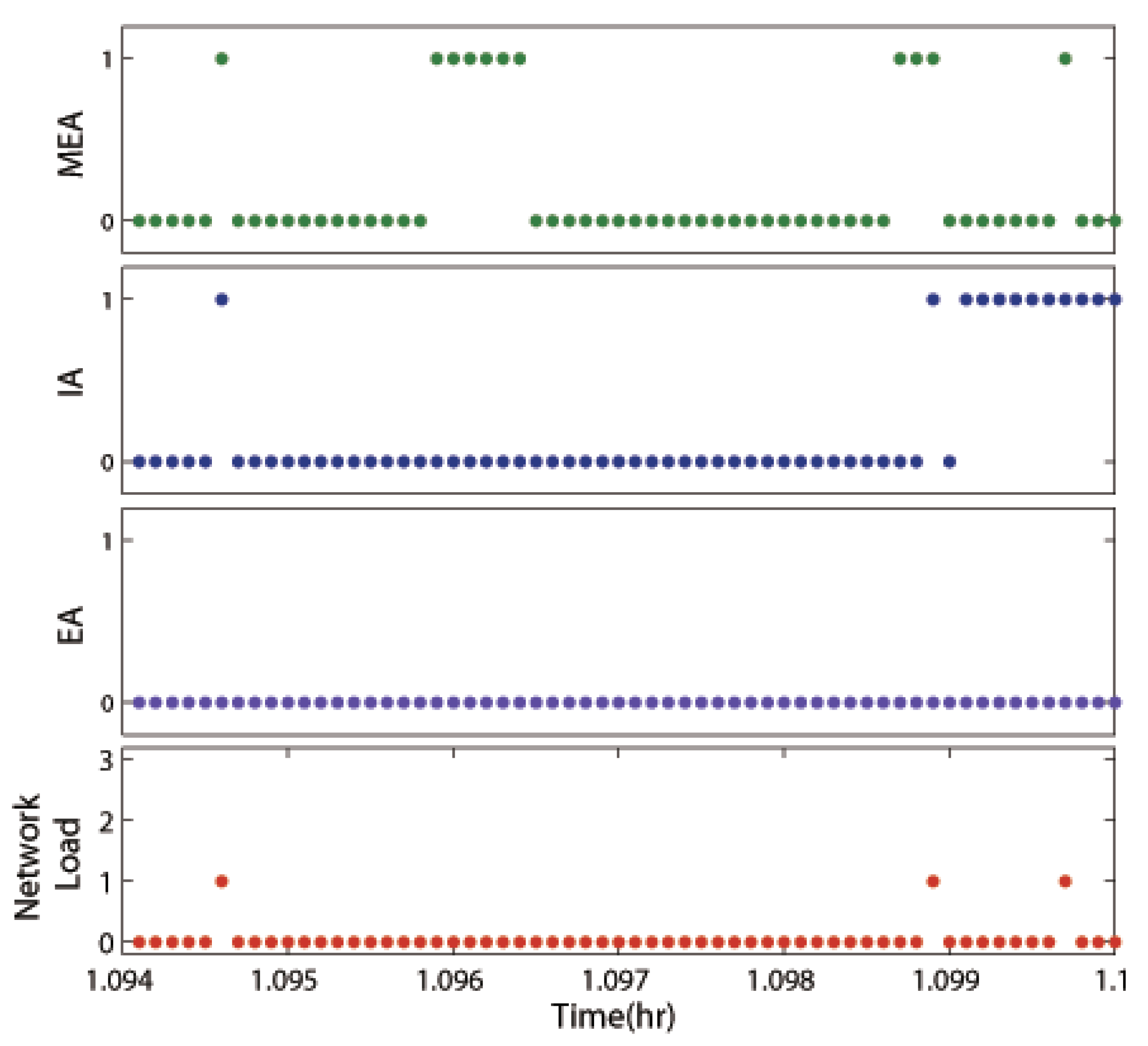
4.1. Case I: No Alarm Signals Reported to the Supervisor (IA = 0, MEA = 0, EA = 0)

This case represents an ideal scenario where (1) all local Lyapunov functions are decreasing under the respective model-based controllers (consistent with the expected local performance and stability requirements); (2) all model state estimation errors stay below the respective thresholds (consistent with the overall stable behavior of the plant as captured by the composite Lyapunov function); and (3) no safety or product quality specifications are violated. In this case, model state updates are not needed and, as a result, the supervisor’s decision is to suspend communication over the network.

4.2. Case II: Only Local Instability Alarms Reported to the Supervisor (IA = 1, MEA = 0, EA = 0)

This case represents a scenario where the stability of at least one subsystem is potentially in jeopardy, but none of the model state estimation error thresholds are breached. This scenario is possible in the event that a local disturbance causes the Lyapunov function for a given subsystem to grow for some time, but this growth is more than offset by the dissipation of the other Lyapunov functions, resulting in a net decay of the composite Lyapunov function. Given that no model state estimation error alarms are reported in this case, the overall closed-loop stability of the plant is not jeopardized as guaranteed by the result of Theorem 1. Consequently, no model state updates are needed, and the supervisor’s decision is to suspend communication over the network. Note that while it may not be possible for the supervisor to identify the cause of the local instability alarms (for example, which subsystems experienced large enough model state estimation errors to cause growth in the Lyapunov functions of the alarm-reporting subsystems), this knowledge is not required for the supervisor’s decision-making process. Furthermore, if this combination of alarm signals persists and model updates continue to be suspended, it is possible that the subsystems reporting the alarms may recover over time.

4.3. Case III: Supervisor Receives Model State Estimation Error Alarms Only (IA = 0, MEA = 1, EA = 0)

In this case, at least one of the plant subsystems reports an alarm to the supervisor indicating a breach of the local model state estimation error threshold; however, no local instability alarms are reported by any of the plant subsystems. While a breach of the specified threshold could signal a potential problem, the fact that the local Lyapunov functions are all decreasing (as indicated by the absence of any local instability alarms) implies that the overall closed-loop system is stable since the composite Lyapunov function is also decreasing at this time. Therefore, no model state updates are necessary and the supervisor suspends information transfer over the network. In such situations and by avoiding these unnecessary updates, the supervisory control approach offers an advantage over unsupervised broadcast-based approaches (e.g., [27]) in which the subsystem breaching the estimation error threshold automatically transmits its state to update its model everywhere in the plant.

4.4. Case IV: Supervisor Receives Both Local Instability and Model State Estimation Error Alarms (IA = 1, MEA = 1, EA = 0)

In this scenario, the fact that the supervisor receives a model state estimation error alarm indicates that the estimation error in at least one subsystem is becoming excessively large. Furthermore, the fact that a local instability alarm is reported to the supervisor indicates that the stability of one or more subsystems is potentially threatened in the sense that the local Lyapunov functions of those subsystems are on the verge of increasing. To address this scenario, the supervisor only prompts the subsystems reporting the model state estimation error alarms to broadcast their state measurements over the network to update their models everywhere and ensure closed-loop stability. Note that restoring communication at this time ensures the continued decay of the composite Lyapunov function, but is not designed to necessarily help (at least not immediately) reverse the detected growth in the local Lyapunov functions since the reported model state estimation error threshold breaches may not be the direct cause for the reported local instability alarms. A causal connection between the two events, however, is not needed for the supervisor to take action. The supervisor’s main objective is to determine whether a given subsystem needs to transmit its data over the network at the time the alarms are reported and to act accordingly.

4.5. Case V: Supervisor Receives Emergency Alarms (EA = 1)

This case includes situations where the local state breaches a certain closed-loop performance bound causing an unacceptable level of performance degradation. The supervisor’s decision in this case is to prompt all subsystems to transmit their data over the network so that all models are updated everywhere in the plant. An example of this is when a given local Lyapunov function begins to increase at some time (e.g., due to an external disturbance), but then, as the supervisor decides not to update any of the models (see Section 4.2), the growth in the local Lyapunov function persists afterwards, causing some desired performance criterion to be violated. An alarm is triggered in this case and sent to the supervisor to report an emergency situation. To maintain the desired closed-loop performance, the supervisor allows all subsystems to communicate with each other to ensure that all models are updated.

An examination of Case V shows that it generally encompasses four possible alarm combinations depending on whether the local instability or model state estimation error alarms are reported along with the emergency alarms. However, among these four, the two combinations with “IA = 0, MEA = 0, EA = 1” and “IA = 0, MEA = 1, EA = 1” are not meaningful. The reason is the fact that, by definition, a local instability alarm is issued whenever the local state is on the verge of escaping a certain neighborhood of the operating steady state. Therefore, an emergency alarm cannot be triggered before a local instability alarm is issued since a breach of the performance bound cannot take place until after the state has escaped the desired neighborhood of the steady state.

The other remaining alarm combinations include “IA = 1, MEA = 0, EA = 1” and “IA = 1, MEA = 1, EA = 1.” In both cases, the supervisor prompts plant-wide communication between all subsystems to avert instabilities and maintain the desired closed-loop performance. The first combination (where IA = 1, MEA = 0, EA = 1), however, is of particular significance since it showcases some of the advantages that the supervisory control strategy has over unsupervised decentralized communication strategies. This combination represents an event where the local state trajectory escapes some desired region around the operating steady state without the supervisor receiving any model state estimation error alarms. By prompting all subsystems to exchange their state measurements to update all models, the supervisor is able to prevent possible performance deterioration. However, in the unsupervised communication approach, no model updates would be triggered in this case (since no model state estimation error alarms are reported), thus leading to performance deterioration.

Remark 5.

In the proposed supervisory control approach, the local control systems are required to communicate with the supervisor each time any of the alarm thresholds are breached. However, what is communicated at those times are the alarm signals only—not the full-state measurements of the constituent subsystems. Whether the state measurements need to be exchanged over the network is dependent on what the appropriate supervisory logic for the given combination of alarms is. In the unsupervised decentralized broadcast-based communication approach, on the other hand, the full-state measurements are always transmitted over the network whenever the local model state estimation error threshold is breached.

Remark 6.

As indicated earlier, the supervisory control approach described in this section was developed under the assumption that the model uncertainties are vanishing. The results can be extended to address the problem of non-vanishing uncertainties. Specifically, one can employ similar Lyapunov calculations to establish new bounds on the dissipation rates of the local Lyapuonv functions and the model state estimation errors that take account of the non-vanishing nature of the uncertainties. These bounds can then serve as new alarm thresholds and be used to adapt the supervisory logic for the various alarm combinations considered previously. In addition to alarm threshold modifications, a key difference between the two cases lies in the type of closed-loop stability that can be enforced. Whereas exponential stability can be achieved under vanishing uncertainties, only ultimate boundedness of the closed-loop state can be enforced under non-vanishing uncertainties. In the latter case, the closed-loop state can be made to converge in finite time to a small terminal neighborhood of the origin. The existence of a terminal set needs to be taken into account in the implementation of the supervisory control approach. Specifically, the fact that no guarantees can be made about the dissipation of the Lyapunov function within the terminal set (even when continuous communication is allowed) suggests that the alarm thresholds developed on the basis of those guarantees are not an appropriate basis for the implementation of the supervisory logic inside the terminal set. One way to address this problem is to locate where the state is at any given time and apply the newly adapted supervisory logic only at the times that the closed-loop state lies outside the terminal set. Once the closed-loop state is within the terminal set, however, communication is suspended until (and unless) the closed-loop state attempts to escape the terminal set.

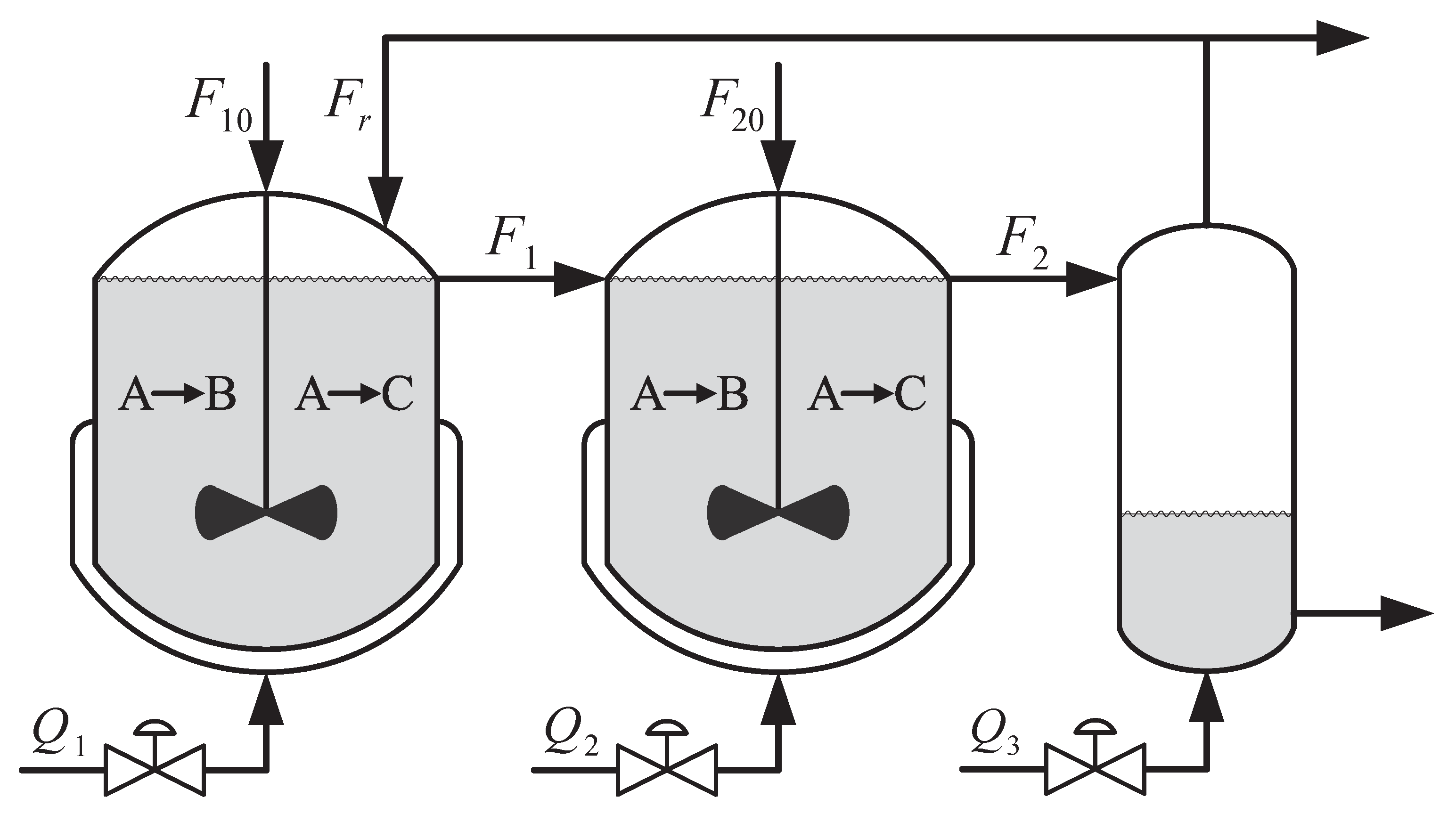
5. Case Study: Application to a Reactor-Separator Network

The objective of this section is to demonstrate an application of the supervisory event-triggered control strategy described in the previous section to a representative chemical process network that consists of a cascade of two continuous stirred tank reactors (CSTRs) connected in series with a flash separator, as shown in Figure 2. The following process dynamic model can be obtained by applying standard material and energy balances [12]:

$$\begin{array}{cc}\hfill {\dot{T}}_1& =\frac{F_{10}}{V_1}(T_{10}-T_1)+\frac{F_r}{V_1}(T_3-T_1)+\sum _{i=1}^2{R}_i(T_1,C_{A1})+\frac{Q_1}{\rho C_p{V}_1}\hfill \\ \hfill {\dot{C}}_{A1}& =\frac{F_{10}}{V_1}(C_{A10}-C_{A1})+\frac{F_r}{V_1}(C_{Ar}-C_{A1})-\sum _{i=1}^2{G}_i(T_1,C_{A1})\hfill \\ \hfill {\dot{C}}_{B1}& =\frac{-F_{10}}{V_1}{C}_{B1}+\frac{F_r}{V_1}(C_{Br}-C_{B1})+k_1{e}^{-E_1/R{T}_1}{C}_{A1}\hfill \\ \hfill {\dot{C}}_{C1}& =\frac{-F_{10}}{V_1}{C}_{C1}+\frac{F_r}{V_1}(C_{Cr}-C_{C1})+k_2{e}^{-E_2/R{T}_1}{C}_{A1}\hfill \\ \hfill {\dot{T}}_2& =\frac{F_1}{V_2}(T_1-T_2)+\frac{F_{20}}{V_2}(T_{20}-T_2)+\sum _{i=1}^2{R}_i(T_2,C_{A2})\hfill \\ \hfill {\dot{C}}_{A2}& =\frac{F_1}{V_2}(C_{A1}-C_{A2})+\frac{F_{20}}{V_2}(C_{A20}-C_{A2})-\sum _{i=1}^2{G}_i(T_2,C_{A2})\hfill \\ \hfill {\dot{C}}_{B2}& =\frac{F_1}{V_2}(C_{B1}-C_{B2})+\frac{F_{20}}{V_2}{C}_{B2}+k_1{e}^{-E_1/R{T}_2}{C}_{A2}+\frac{Q_2}{\rho C_p{V}_2}\hfill \\ \hfill {\dot{C}}_{C2}& =\frac{F_1}{V_2}(C_{C1}-C_{C2})+\frac{F_{20}}{V_2}{C}_{C2}+k_2{e}^{-E_2/R{T}_2}{C}_{A2}\hfill \\ \hfill {\dot{T}}_3& =\frac{F_2}{V_3}(T_2-T_3)+\frac{H_{vap}{F}_r}{\rho C_p{V}_3}+\frac{Q_3}{\rho C_p{V}_3}\hfill \\ \hfill {\dot{C}}_{A3}& =\frac{F_2}{V_3}(C_{A2}-C_{A3})-\frac{F_r}{V_3}(C_{Ar}-C_{A3})\hfill \\ \hfill {\dot{C}}_{B3}& =\frac{F_2}{V_3}(C_{B2}-C_{B3})-\frac{F_r}{V_3}(C_{Br}-C_{B3})\hfill \\ \hfill {\dot{C}}_{C3}& =\frac{F_2}{V_3}(C_{C2}-C_{C3})-\frac{F_r}{V_3}(C_{Cr}-C_{C3})\hfill \end{array}$$

where $T_j$, $C_{Aj}$, $Q_j$, and $V_j$ are, respectively, the temperature, the reactant concentration, the rate of heat input, and the volume of the j-th vessel, for $j\in \{1,2,3\}$; $C_{Bj}$ and $C_{Cj}$ denote the product concentrations; $R_i(T_j,C_{Aj})=\frac{-▵H_i}{\rho C_p}{k}_i{e}^{-E_i/R{T}_j}{C}_{Aj}$ and $G_i(T_j,C_{Aj})=e^{-E_i/R{T}_j}{C}_{Aj}$, are the reaction rate expressions for the first and second reactions, respectively; $F_{j0}$ denotes the flow rate of a fresh feed stream associated with the j-th vessel, with temperature $T_{j0}$ and reactant concentration $C_{Aj0}$; $F_j$ denotes the flow rate of the outlet stream of the j-th vessel; $F_r$ is the recycle flow rate; $▵H$, $k_i$, $E_i$, $i\in \{1,2\}$, are, respectively, the enthalpies, pre-exponential constants and activation energies of the two reactions; $C_p$ and $\rho$ denote the heat capacity and density, respectively; and $H_{vap}$ is the heat of vaporization.

The control problem under consideration is to stabilize the process near the open-loop unstable steady state ($T_1=369.6\mathrm{K}$, $T_2=435.3\mathrm{K}$, $T_3=435.3\mathrm{K}$) using the heat transfer rates, $Q_j$, $j\in \{1,2,3\}$, as the manipulated inputs. This objective is to be achieved while keeping the rate of measurement transfer between the three subsystems to a minimum. To address the problem, we initially synthesized, and properly tuned, for each subsystem, a nonlinear Lyapunov-based feedback controller to achieve the stabilization objective under continuous communication between the plant subsystems. Extensive simulations of the closed-loop system were performed, for various initial conditions, to verify that the three controllers robustly stabilize the closed-loop system around the operating steady state.

To address the problem when state measurements are transmitted only at discrete times over plant-wide communication network, uncertain models of all three subsystems were included in each local control system. The heats of reactions were considered to be the uncertain parameters in each model. As noted in Remark 3, having each unit include a copy of its own model enables the unit to track its own model state estimation error in all subsystems. Taking subsystem 1 as an example, in the control system of CSTR 1, models of units 1, 2, and 3 (i.e., CSTR 1, CSTR 2, and the flash vessel) are all embedded. An estimate of ${\mathbf{x}}_1$ is provided by a model of the form:

$${\dot{\widehat{\mathbf{x}}}}_1={\widehat{\mathbf{f}}}_1({\widehat{\mathbf{x}}}_1,{\widehat{\mathbf{x}}}_2,{\widehat{\mathbf{x}}}_3)+{\widehat{\mathbf{G}}}_1{\mathbf{u}}_1({\widehat{\mathbf{x}}}_1,{\widehat{\mathbf{x}}}_2,{\widehat{\mathbf{x}}}_3)$$

Note that even though it is assumed that local measurements are transmitted to the local controller via dedicated links, meaning ${\mathbf{x}}_1$ is continuously accessible to controller 1, ${\widehat{\mathbf{x}}}_1$ is used for controller implementation instead of ${\mathbf{x}}_1$ for the purpose of having the closed-loop model of CSTR 1 to be identical in all three units. Controller 1 computes its model state estimation error by comparing ${\widehat{\mathbf{x}}}_1$ and ${\mathbf{x}}_1$. When the model of CSTR 1 is updated at some time $t_s$, we have ${\widehat{\mathbf{x}}}_1\left(t_s\right)={\mathbf{x}}_1\left(t_s\right)$, and therefore ${\mathbf{e}}_1\left(t_s\right)=0$ in all subsystems.

In the remainder of this section, we present an assessment of the performance of the proposed supervisory control approach under different scenarios. We start in Section 5.1, where the implementation of the supervisory control logic is illustrated for a case when an unexpected disturbance in the feed composition takes place. Section 5.2 then presents a comparison between the performances of the supervisory control approach and the unsupervised broadcast-based approach for a case when an unexpected disturbance in the feed temperature occurs. Finally, Section 5.3 evaluates the performance of both the supervised and unsupervised communication strategies when input rate constraints are considered.

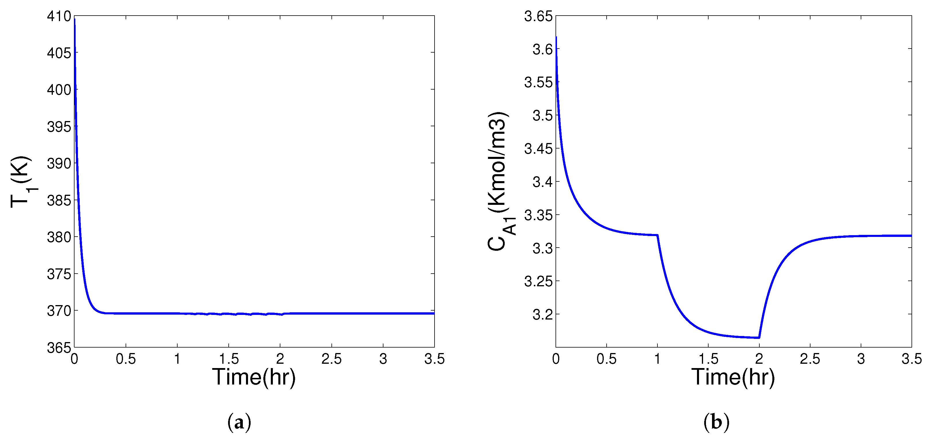
5.1. Implementation of Supervisory Control Approach under Disturbances

In this part, we assess the effectiveness of the supervisory controller in meeting the control and communication objectives when unanticipated external disturbances are introduced. To this end, it was first verified that, in the absence of external disturbances, the local controllers stabilize the closed-loop system near the desired steady state. To simulate external disturbances, a pulse disturbance in the inlet concentration of the reactant species, where $C_{A10}$ drops from $4.0\mathrm{Kmol}/{\mathrm{m}}^3$ to $3.8\mathrm{Kmol}/{\mathrm{m}}^3$, was introduced for all times in the interval $t\in [1,2]$ h.

Figure 3 depicts the evolution of the closed-loop reactor temperature and reactant concentration profiles for CSTR 1. The disturbance’s impact on the closed-loop system can be seen in Figure 3b, where following the onset of the disturbance, the reactant concentration deviates from the desired operating steady state for some time until the disturbance is over, at which time the reactant concentration is gradually restored to the desired operating point. It can be seen from Figure 3a that the reactor temperature, which exhibits faster closed-loop dynamics, is not significantly impacted by the disturbance.

Figure 4 shows the frequency and types of alarms that the supervisor receives—as well as the corresponding network load—during a representative time interval following the onset of the disturbance, $[1.094,1.1]$ h. Here, the network load at each time is defined as the number of subsystems that transmit their measurements over the network at that time (i.e., the units that are actively utilizing the network). For example, at time $t=1.0946$ h, the supervisor receives both model state estimation error and local instability alarms, but no emergency alarms, as shown by the top three plots in Figure 4. Based on the supervisory control logic presented in Section 4.4, the supervisor prompts the subsystem reporting the model state estimation error alarm to send its measurements over the network to update its model in all three subsystems. The network load plot shows that one model is updated.

Following this event, the supervisor receives no alarms, and communication remains suspended until $t=1.0959$ h. Over the next time interval $[1.0959,1.0964]$ h, the supervisor continuously receives model state estimation error alarms; however, no instability or emergency alarms are reported. Based on the supervisory logic presented in Section 4.3, the supervisor decides to keep the communication suspended (note that the model updates would have been triggered during this interval had the unsupervised proactive communication approach been used). The next time a model update is triggered by the supervisor occurs at $t=1.0989$ h when both local instability and model state estimation error alarms are received. During the subsequent interval $[1.0991,1.0996]$ h, only local instability alarms are received by the supervisor, with neither model state estimation error alarms nor emergency alarms being reported. As a result, the supervisor decides not to trigger any model updates over this interval. Immediately after this interval, however, both local instability and model state estimation error alarms are reported at $t=1.0997$ h. The supervisor restores communication at this time to allow a model update for the third and last time during this interval. Figure 3 and Figure 4 show that the supervisory control logic successfully achieves the control objective while keeping the network load to a minimum.

5.2. Comparison between Supervised and Unsupervised Broadcast-Based Communication Strategies

The objective of this section is to compare the supervisory control approach with the unsupervised broadcast-based communication approach in terms of the achievable closed-loop performance and network utilization rates. To this end, we simulate a situation in which an emergency alarm is reported to the supervisor, and introduce a significant pulse disturbance in the feed temperature of CSTR 1, $T_{10}$, at $t=1.0$ h after the process has settled at the desired steady state. The pulse disturbance is simulated by increasing the feed temperature from its nominal value of $300K$ to $350K$ during the interval $[1,2]$ h.

Figure 5 depicts the closed-loop reactor temperature and reactant concentration profiles for CSTR1. The performance obtained under the supervisory control approach is depicted by the solid (blue) profiles, whereas the performance obtained under the unsupervised broadcast-based communication strategy is shown by the dashed (red) profiles. Due to the strong impact of the disturbance, the process states in both cases deviate from the desired steady state for some time before converging back after the disturbance is over. However, the observed deviation is less severe when the supervisory controller is implemented.

The contrasting behaviors can be understood in reference to the alarm signals and network load shown in Figure 6. It can be seen that a persistent emergency alarm is triggered and reported to the supervisor starting at $t=1.3877$ h, and as a result, the supervisor prompts all three subsystems to transmit their measurements to update all three models according to the appropriate supervisory logic for this case (see Section 4.5). This decision results in a sustained increase in the model update frequency (and hence the network load) which helps reduce the deviation of the process states from the desired operating point during the disturbance event. Note that no model state estimation error alarms are reported during this interval, and therefore, the unsupervised broadcast-based communication strategy does not trigger any communication or model updates in response to the disturbance, leading to more performance degradation.

5.3. Supervisory Event-Based Controller Implementation under Input Rate Constraints

As discussed earlier, the supervisory event-triggered control approach is capable of reducing the unnecessary transmission of state information between plant subsystems and therefore generally helps reduce the rate at which the models need to be updated. Notice that whenever a model state is updated or reset, the inconsistency in the computed control action results in a sudden change in the actuator output. To protect actuators from wear and tear and prolong their service life, a lower model update rate is generally desired, as long as the control objectives can be fulfilled. The simulation scenarios considered thus far did not consider the issue of input rate constraints. In practice, the rate of change in the manipulated input cannot be arbitrarily large due to the physical limitations associated with the actuators. In this subsection, we evaluate the performance of the supervisory control system when constraints on the input rate are considered.

For simulation purposes, a rate constraint of $|d{Q}_i|\le 1000$ KJ/h, $i\in \{1,2,3\}$, over one time step is considered. To suppress the influence of transient states, all subsystems are initialized at the operating steady state. A pulse disturbance in the feed concentration is introduced for $t\in [1,2]$ h.

Table 1. A comparison between the supervisory control approach and the unsupervised broadcast-based communication approach in terms of the resulting model update and hit-bound frequencies in the presence and absence of input rate constraints.

	Constraint	Update Frequency (%)				Hit Bound Frequency (%)
		CSTR 1	CSTR 2	Flash Unit	Overall
Supervisory control	✕	$2.0\times {10}^{-2}$	$2.0\times {10}^{-2}$	$2.9\times {10}^{-3}$	$4.3\times {10}^{-2}$	-
approach	✔	$2.0\times {10}^{-2}$	$2.0\times {10}^{-2}$	$2.9\times {10}^{-3}$	$4.3\times {10}^{-2}$	2.97
Broadcast-	✕	$7.7\times {10}^{-2}$	0.23	$7.7\times {10}^{-2}$	0.38	-
based approach	✔	$8.0\times {10}^{-2}$	0.24	0.13	0.45	3.38

compares the resulting update rates of the individual units, as well as the overall update rate, for the case when the input rate constraints are enforced (this case is marked by the check mark) and the case when they are not enforced (this case is marked by the x mark). The update rate for an individual subsystem is defined as the ratio of the number of time instances that a subsystem transmits its data to the total number of time instances in a given time interval. The overall update rate is simply the sum of the three update rates.

It can be observed that the update rates under the supervisory event-triggered control approach do not change much with or without the input rate constraints in place. However, when the unsupervised broadcast-based approach is implemented, enforcing input rate constraints causes the update rates to increase appreciably as a result of the increased communication rate. Another point of comparison between the two approaches is the hit-bound-frequency, which refers to the number of instances that the change in input exceeds the imposed constraint over the given interval. This frequency is lower under the supervisory control approach. The reason is the fact that the unsupervised broadcast-based approach leads to more unnecessary model updates and thus causes the control action to more frequently hit the rate constraints, which leads to further errors in the control action implemented and an increased update rate to try to compensate for these errors. On the other hand, by requiring fewer updates, the supervisory control approach avoids having frequent jumps in the control signal, and thus avoids violating the input rate constraints as much as possible, and is able to keep the communication rate at a lower level.

The difference between the two approaches with respect to their network resource utilization levels has important implications not only for the network load, but also for the ability of the control system to enforce the desired closed-loop stability and performance properties. To illustrate this point, we consider a case where the input rate constraints are much tighter than considered in the previous scenario. Specifically, we consider a rate constraint of $|d{Q}_i|\le 48$ KJ/h over a single time step. A pulse disturbance in the feed concentration (similar to that considered in Section 5.1) is introduced for one hour starting at $t=1.0$ h.

Figure 7 shows the resulting closed-loop profiles of the reactant concentration and the rate of heat transfer for CSTR 1 under the supervisory control approach (solid blue) and under the unsupervised broadcast-based approach (dashed red). It can be seen that the latter approach is unable to maintain stability and leads to significant performance deterioration, whereas the supervisory control approach manages to stabilize the closed-loop system near the desired steady state once the disturbance is terminated. This behavior is explained by the fact that, under the unsupervised broadcast-based communication strategy, the change in the rate of heat transfer more frequently breaches the constraints (due to the increased model update rate) and eventually becomes saturated near the end of the disturbance period and remains saturated thereafter. This limits the cooling rate, as shown by the red straight line in Figure 7b. The actuator fails to cool down the reactor sufficiently quickly, leading to a prolonged period of high temperature and reactant depletion even after the disturbance is removed. By contrast, the supervisory control approach is able to avoid this problem by limiting the number of unnecessary model updates which helps avoid frequent breaches of the input rate constraints.

6. Conclusions

This work considered the problem of resource-aware control of a class of large-scale systems controlled over communication networks, subject to model uncertainty and communication rate constraints. A supervisory control system that employs event-triggered communication logic was designed to achieve closed-loop stability while also optimizing the network load. The design methodology was realized by initially synthesizing a family of local model-based controllers that communicate with each other at discrete times over the network. Lyapunov techniques were then used to derive appropriate stability and performance thresholds for each subsystem which were used as alarm triggers for communication between the local control systems and the supervisor. The supervisor was tasked with managing the alarm signals transmitted by the constituent subsystems and employed logical operations to decide which subsystems can access the network at any given time. Various alarm combinations were considered and analyzed, and a discussion of the appropriate supervisory control action in each case was presented. The implementation of the supervisory control approach was illustrated using a benchmark chemical process example, and compared with unsupervised event-based communication approaches.

The main advantage of the developed supervisory control approach is its ability to balance the overall closed-loop stability objective with the need to maintain acceptable levels of performance locally, while optimizing the rate of data transfer between the local control systems. As demonstrated in the simulation study, this leads to a more judicious utilization of network resources that results in improved closed-loop performance (compared with decentralized communication schemes) when the process is subject to unexpected external disturbances and input rate constraints. As is the case with any model-based control approach, the design and implementation of the proposed supervisory control system requires the availability of appropriate models that capture the dynamics of component subsystems, as well as an explicit characterization of the model uncertainty bounds. In this study, it was also assumed that full-state measurements are available and that the communication links between the supervisor and the plant subsystems are ideal in the sense that communication disruptions due to time delays and data losses are negligible. Future research directions include extending the proposed supervisory control structure to address these practical implementation issues, including the availability of only partial state measurements and the presence of communication delays and data losses in the communication links.

References

1. Cui, H.; Jacobsen, E.W. Performance limitations in decentralized control. J. Proc. Contr. 2002, 12, 485–494. [Google Scholar] [CrossRef]
2. Kordestani, M.; Safavi, A.A.; Saif, M. Recent Survey of Large-Scale Systems: Architectures, Controller Strategies, and Industrial Applications. IEEE Syst. J. 2021, 15, 5440–5453. [Google Scholar] [CrossRef]
3. Svoboda, F.; Hengster-Movric, K.; Hromčík, M. Decentralized control for large scale systems with inherently coupled subsystems. J. Vib. Control. 2021. [Google Scholar] [CrossRef]
4. Tharanidharan, V.; Sakthivel, R.; Shanmugam, H.; Almakhles, D.J. Decentralized observer-based controller design for large-scale systems with quantized measurements and actuator faults. Asian J. Control. 2022, 1–11. [Google Scholar] [CrossRef]
5. Jogwar, S.; Baldea, M.; Daoutidis, P. Dynamics and control of process networks with large energy recycle. Ind. Eng. Chem. Res. 2009, 48, 6087–6097. [Google Scholar] [CrossRef]
6. Debnath, S.; Sahoo, S.R.; Decardi-Nelson, B.; Liu, J. Subsystem decomposition and distributed state estimation of nonlinear processes with implicit time-scale multiplicity. Aiche J. 2022, 68, e17661. [Google Scholar] [CrossRef]
7. Jillson, K.R.; Ydsite, B.E. Process networks with decentralized inventory and flow control. J. Proc. Contr. 2007, 17, 399–413. [Google Scholar] [CrossRef]
8. Zheng, C.; Tippett, M.; Bao, J.; Liu, J. Dissipativity-based distributed model predictive control with low rate communication. AIChE J. 2015, 61, 3288–3303. [Google Scholar] [CrossRef]
9. Aboudonia, A.; Martinelli, A.; Lygeros, J. Passivity-based Decentralized Control for Discrete-time Large-scale Systems. In Proceedings of the American Control Conference, Philadelphia, PA, USA, 25–28 May 2021; pp. 2037–2042. [Google Scholar]
10. Tetiker, M.D.; Artel, F.; Cinar, A. Control of grade transitions in distributed chemical reactor networks: An agent-based approach. Comp. Chem. Eng. 2008, 32, 1984–1994. [Google Scholar] [CrossRef]
11. Chen, F.; Ren, W. On the Control of Multi-Agent Systems: A Survey. Found. Trends Syst. Control. 2019, 6, 339–499. [Google Scholar] [CrossRef]
12. Christofides, P.D.; Liu, J.; de la Pena, D.M. Networked and Distributed Predictive Control: Methods and Nonlinear Process Network Applications; Springer: London, UK, 2011. [Google Scholar]
13. Cai, X.; Tippett, M.; Xie, L.; Bao, J. Fast distributed MPC based on active set method. Comp. Chem. Eng. 2014, 71, 158–170. [Google Scholar] [CrossRef]
14. Coordinating distributed MPC efficiently on a plant-wide scale: The Lyapunov envelope algorithm. Comput. Chem. Eng. 2021, 155, 107532. [CrossRef]
15. Christofides, P.D.; Davis, J.; El-Farra, N.H.; Clark, D.; Harris, K.; Gipson, J. Smart plant operations: Vision, progress and challenges. AIChE J. 2007, 53, 2734–2741. [Google Scholar] [CrossRef]
16. El-Farra, N.H.; Christofides, P.D. Speical issue on control and optimization of smart plant operations. Chem. Eng. Sci. 2015, 136, 1. [Google Scholar] [CrossRef]
17. Zhang, D.; Shi, P.; Wang, Q.G.; Yu, L. Analysis and synthesis of networked control systems: A survey of recent advances and challenges. ISA Trans. 2017, 66, 376–392. [Google Scholar] [CrossRef]
18. Ge, X.; Yang, F.; Han, Q.L. Distributed networked control systems: A brief overview. Inf. Sci. 2017, 380, 117–131. [Google Scholar] [CrossRef]
19. Zhou, W.; Wang, Y.; Liang, Y. Sliding mode control for networked control systems: A brief survey. ISA Trans. 2021, 124, 249–259. [Google Scholar] [CrossRef] [PubMed]
20. Sandberg, H.; Gupta, V.; Johansson, K.H. Secure Networked Control Systems. Annu. Rev. Control. Robot. Auton. Syst. 2022, 5, 445–464. [Google Scholar] [CrossRef]
21. Chanfreut, P.; Maestre, J.M.; Camacho, E.F. A survey on clustering methods for distributed and networked control systems. Annu. Rev. Control. 2021, 52, 75–90. [Google Scholar] [CrossRef]
22. Gautam, M.K.; Pati, A.; Mishra, S.K.; Appasani, B.; Kabalci, E.; Bizon, N.; Thounthong, P. A comprehensive review of the evolution of networked control system technology and its future potentials. Sustainability 2021, 13, 2962. [Google Scholar] [CrossRef]
23. Wu, J.; Peng, C.; Yang, H.; Wang, Y.L. Recent advances in event-triggered security control of networked systems: A survey. Int. J. Syst. Sci. 2022, 23, 1–20. [Google Scholar] [CrossRef]
24. Sun, Y.; El-Farra, N.H. Quasi-decentralized model-based networked control of process systems. Comput. & Chem. Eng. 2008, 32, 2016–2029. [Google Scholar]
25. Sun, Y.; El-Farra, N.H. Quasi-decentralized networked process control using an adaptive communication policy. In Proceedings of the American Control Conference, Baltimore, MA, USA, 30 June–2 July 2010; pp. 2841–2846. [Google Scholar]
26. Wang, X.; Lemmon, M. Event-triggering in distributed networked control systems. IEEE Trans. Autom. Control. 2011, 56, 586–601. [Google Scholar] [CrossRef] [Green Version]
27. Garcia, E.; Cao, Y.; Yu, H.; Antsaklis, P.; Casbeer, D. Decentralised event-triggered cooperative control with limited communication. Int. J. Control. 2013, 86, 1479–1488. [Google Scholar] [CrossRef]
28. Garcia, E.; Antsaklis, P.J. Model-based event-triggered control for systems with quantization and time-varying network delays. IEEE Trans. Autom. Control. 2013, 58, 422–434. [Google Scholar] [CrossRef]
29. Xue, D.; El-Farra, N.H. Supervisory logic for control of networked process systems with event-based communication. In Proceedings of the American Control Conference, Boston, MA, USA, 6–8 July 2016; pp. 7135–7140. [Google Scholar]
30. Khalil, H.K. Nonlinear Systems, 2nd ed.; Prentice Hall: Upper Saddle River, NJ, USA, 1996. [Google Scholar]
31. Christofides, P.D.; El-Farra, N.H. Control of Nonlinear and Hybrid Process Systems: Designs for Uncertainty, Constraints and Time-Delays; Springer: Berlin, Germany, 2005. [Google Scholar]
32. Zhang, J.; Liu, S.; Li, L.; Feng, Q. The KKT optimality conditions in a class of generalized convex optimization problems with an interval-valued objective function. Optim. Lett. 2014, 8, 607–631. [Google Scholar] [CrossRef]
33. Treanţă, S. Robust saddle-point criterion in second-order partial differential equation and partial differential inequation constrained control problems. Int. J. Robust Nonlinear Control. 2021, 31, 9282–9293. [Google Scholar] [CrossRef]
34. Treanţă, S. Efficiency in uncertain variational control problems. Neural Comput. Appl. 2021, 33, 5719–5732. [Google Scholar] [CrossRef]
Figure 1. A schematic representation of the supervisory event-triggered control structure for a process network comprised of three subsystems.
Mathematics 10 01964 g001
Figure 2. An example process network comprised of two continuous stirred tank reactors and a flash separator.
Mathematics 10 01964 g002
Figure 3. Evolution of the closed-loop temperature (a) and the reactant concentration (b) in CSTR 1 under the supervisory control approach in the presence of a pulse disturbance in the feed concentration.
Mathematics 10 01964 g003
Figure 4. Status of the alarm signals showing the times when the various event alarms are reported to the supervisor and the resulting network load when the supervisory event-triggered communication strategy is implemented under a disturbance in the feed concentration. The model state estimation error alarms are shown in green, the local instability alarms are shown in blue, and the emergency alarms are shown in purple. The network load is shown in red.
Mathematics 10 01964 g004
Figure 5. Evolution of the closed-loop reactor temperature (a) and reactant concentration (b) in CSTR 1 under the supervisory control approach (solid line) and the unsupervised broadcast-based approach (dashed line) in the presence of a large pulse disturbance in the feed temperature.
Mathematics 10 01964 g005
Figure 6. Status of the alarm signals showing the times when various event alarms are reported to the supervisor and the resulting network load when the supervisory event-triggered communication strategy is implemented under a large disturbance in the feed temperature. The model state estimation error alarms are shown in green, the local instability alarms are shown in blue, and the emergency alarms are shown in purple. The network load is shown in red.
Mathematics 10 01964 g006
Figure 7. A comparison between the evolution of the reactant concentration (a) and the rate of heat transfer (b) for CSTR 1 under the supervisory control approach (solid profiles) and under the unsupervised broadcast-based communication approach (dashed profiles).
Mathematics 10 01964 g007