
A Novel Spatio-Temporal Fully Meshless Method for Parabolic PDEs

 , and
, and
Abstract
| Zum Raum wird hier die Zeit | ||||
| (Here, time becomes space) | ||||
| (Richard Wagner, Parsifal) |
1. Introduction
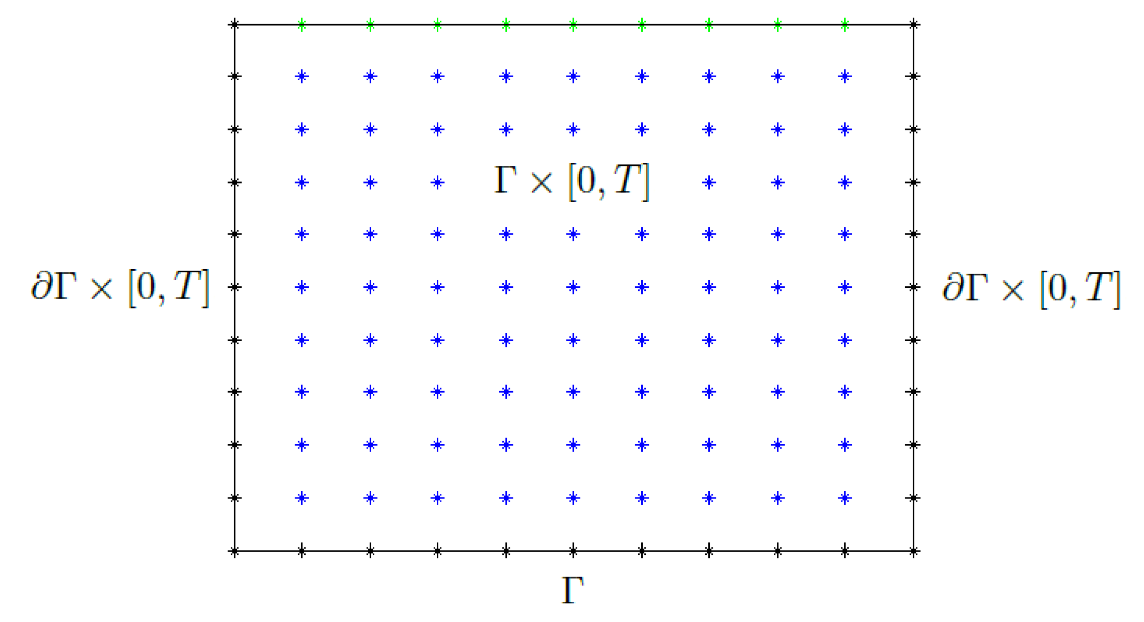
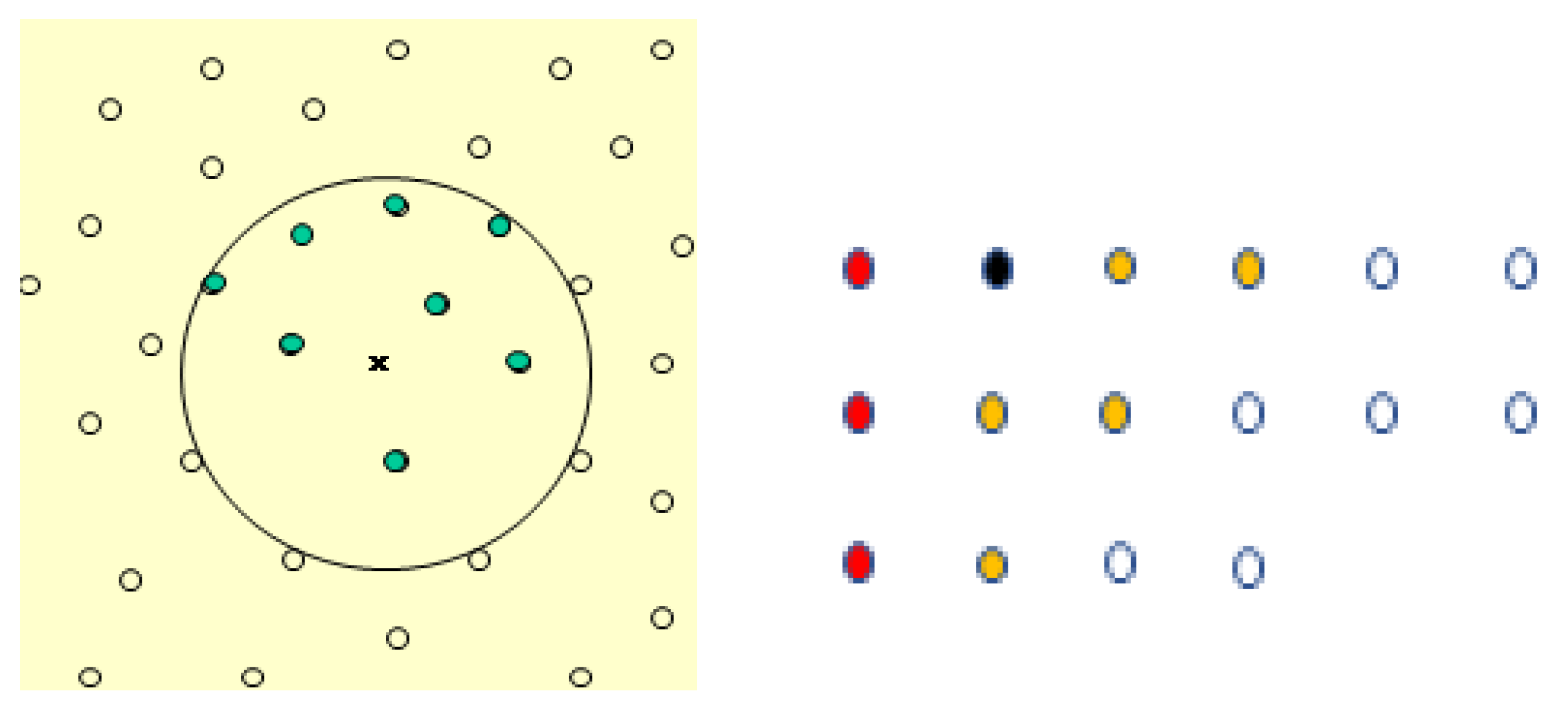
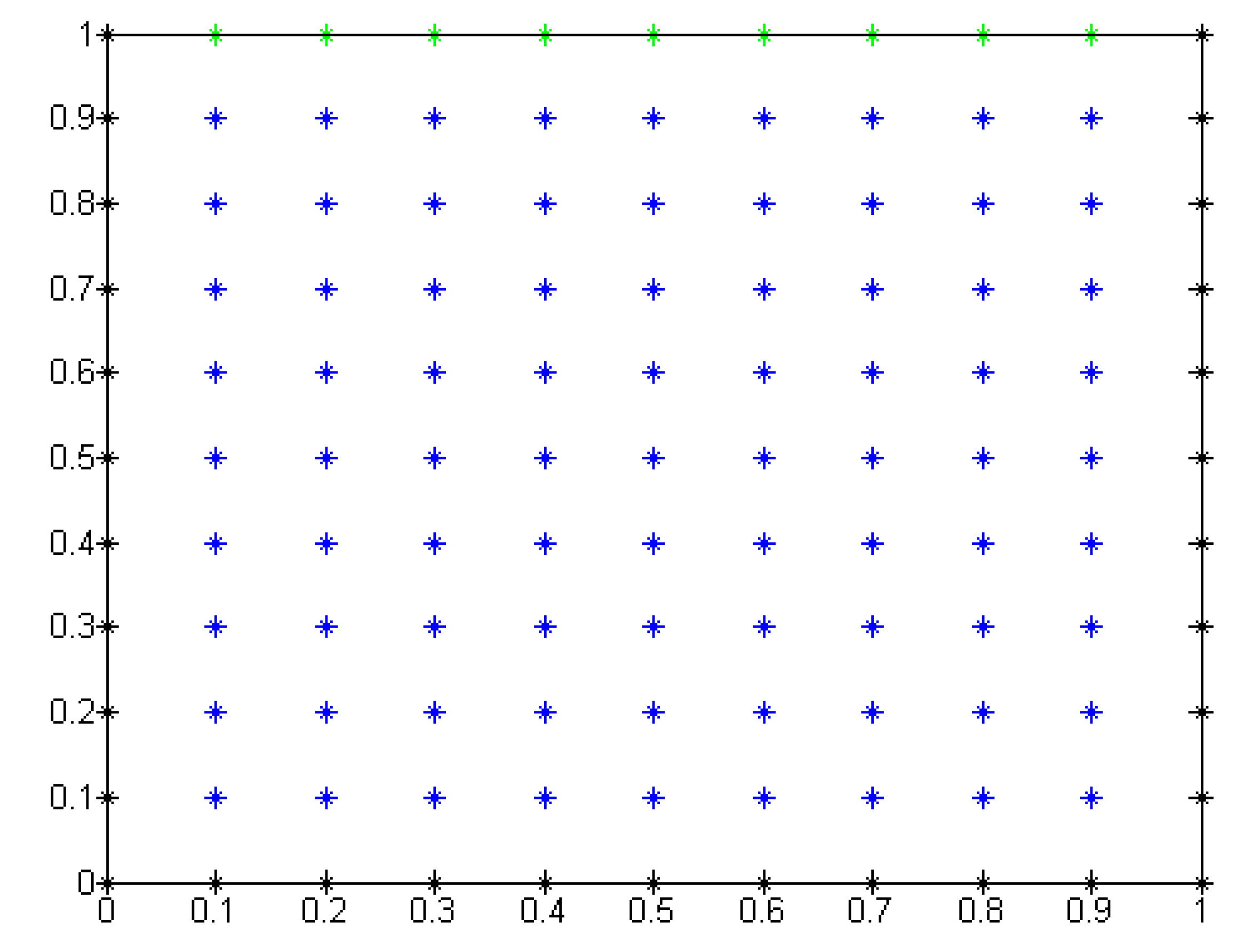
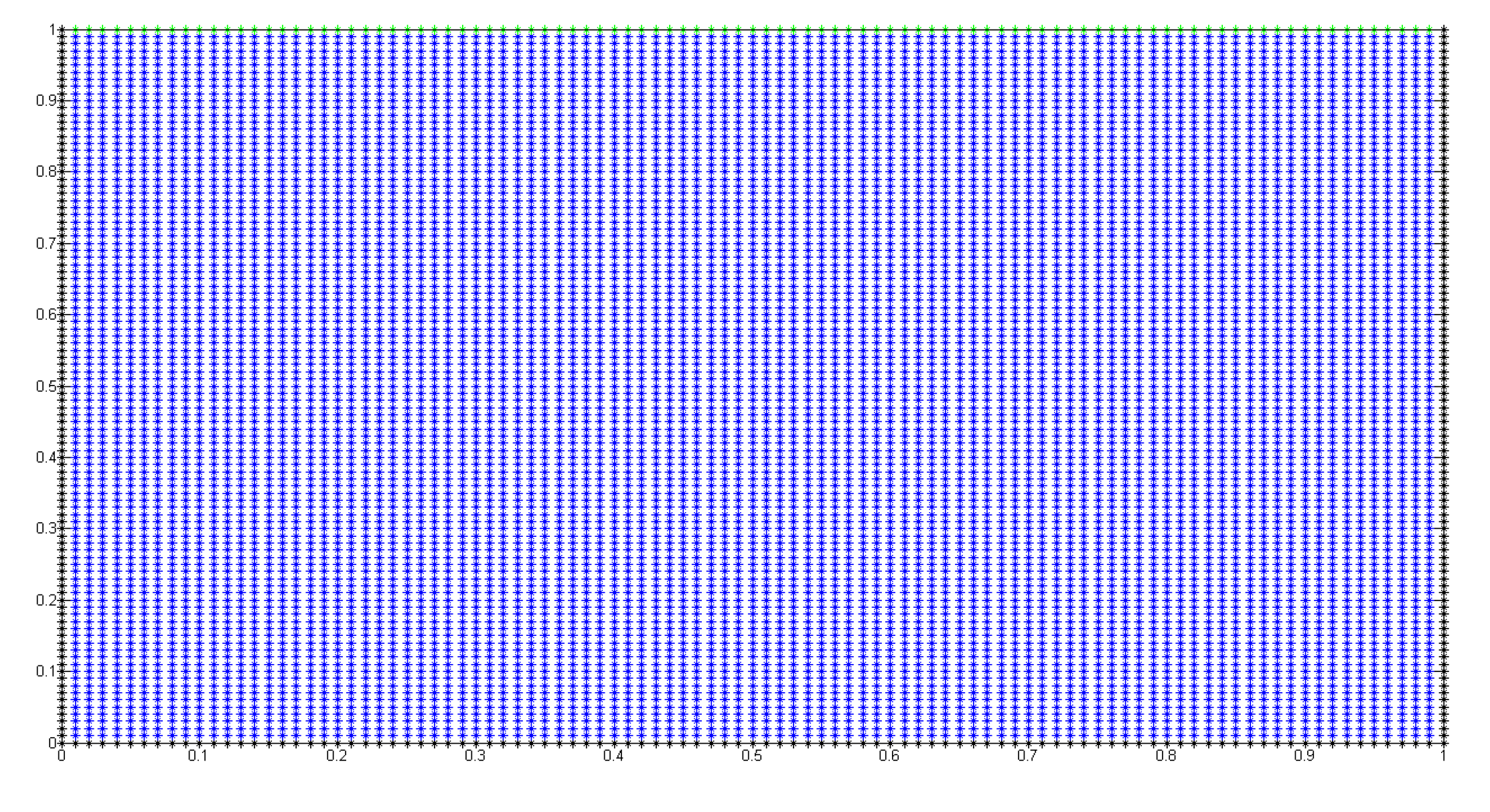
2. Space Time Cloud Method (STCM)
3. Numerical Results
3.1. 2D Problems
3.1.1. Example 1
3.1.2. Example 2
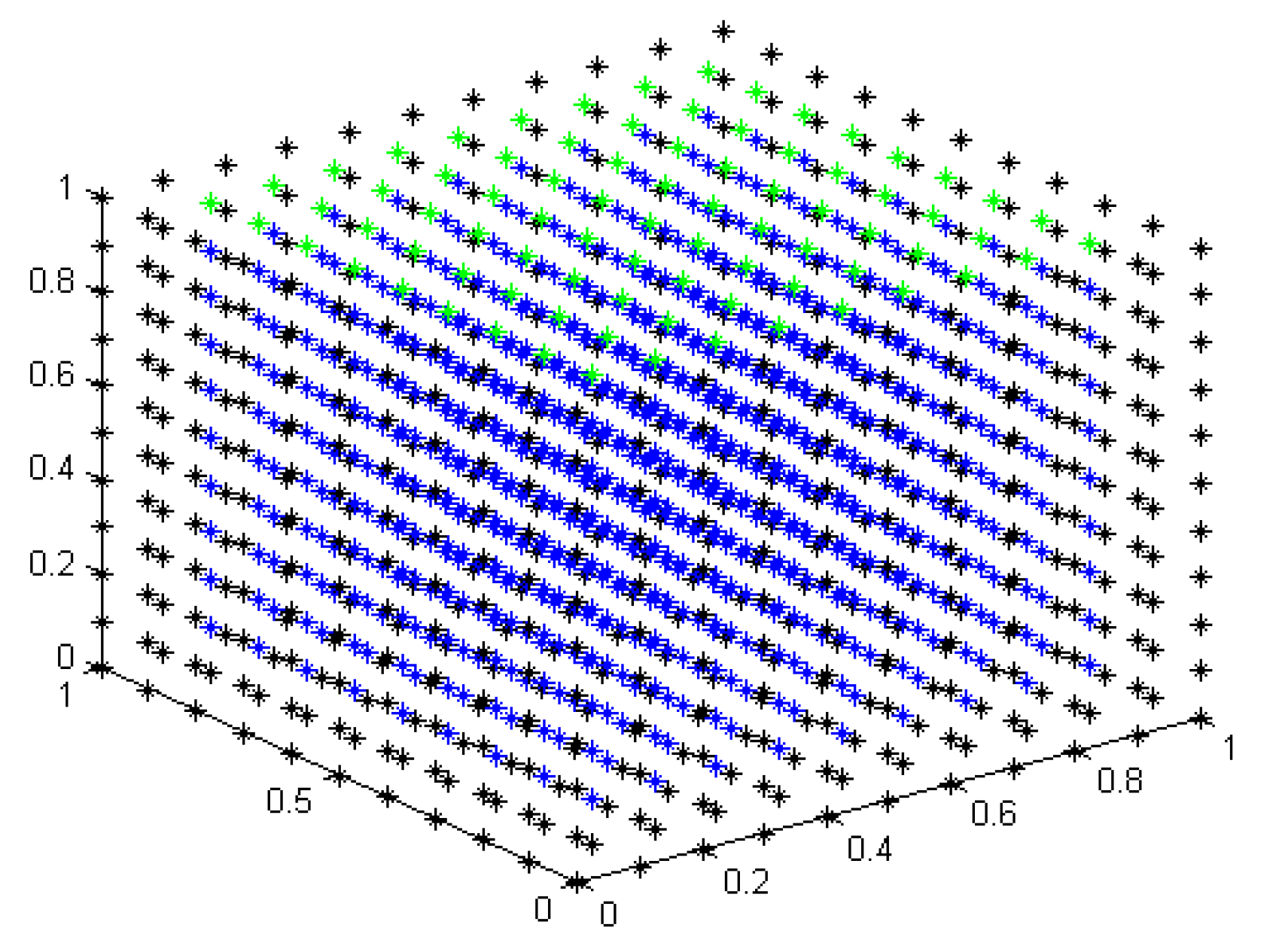
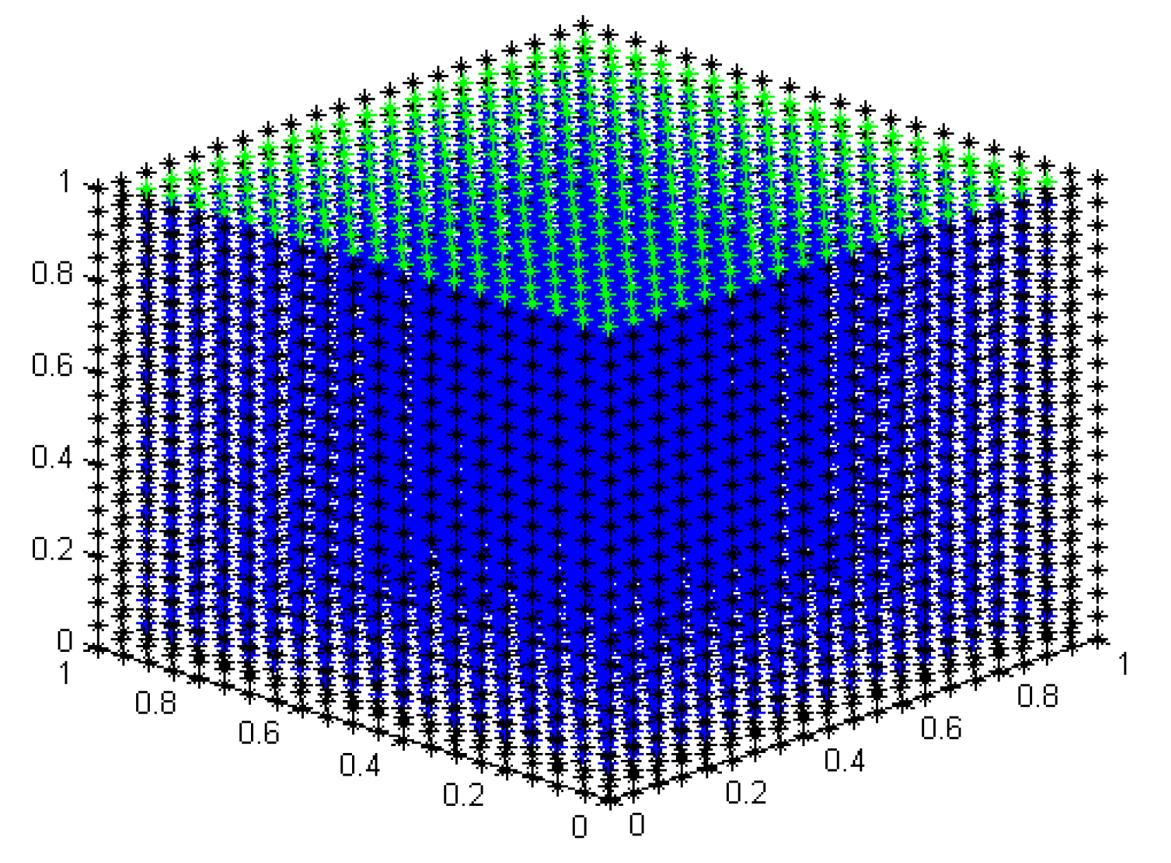
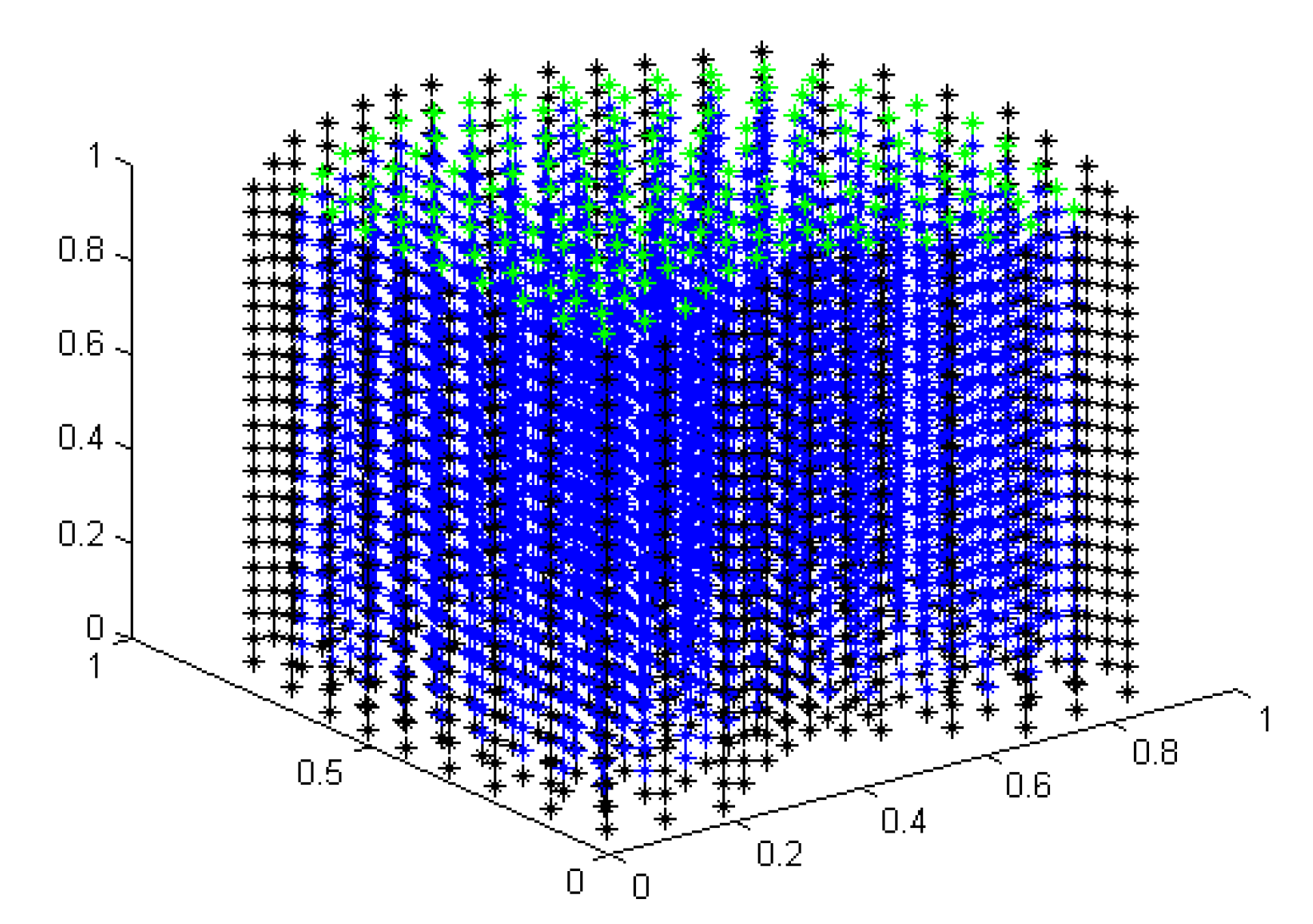
3.2. 3D Problems
3.2.1. Example 3
3.2.2. Example 4
4. Conclusions
Author Contributions
Funding
Institutional Review Board Statement
Informed Consent Statement
Data Availability Statement
Acknowledgments
Conflicts of Interest
References
- Li, S.; Liu, W.K. Meshfree Particle Methods; Springer Science & Business Media: Berlin/Heidelberg, Germany, 2007. [Google Scholar]
- Nguyen, V.P.; Rabczuk, T.; Bordas, S.; Duflot, M. Meshless methods: A review and computer implementation aspects. Math. Comput. Simul. 2008, 79, 763–813. [Google Scholar] [CrossRef]
- Huang, T.H.; Wei, H.; Chen, J.S.; Hillman, M.C. RKPM2D: An open-source implementation of nodally integrated reproducing kernel particle method for solving partial differential equations. Comput. Part. Mech. 2020, 7, 393–433. [Google Scholar] [CrossRef]
- Zhang, C.; Rezavand, M.; Zhu, Y.; Yu, Y.; Wu, D.; Zhang, W.; Wang, J.; Hu, X. SPHinXsys: An open-source multi-physics and multi-resolution library based on smoothed particle hydrodynamics. Comput. Phys. Commun. 2021, 267, 108066. [Google Scholar] [CrossRef]
- Jensen, P.S. Finite difference technique for variable grids. Comput. Struct. 1972, 2, 17–29. [Google Scholar] [CrossRef]
- Liszka, T.; Orkisz, J. The finite difference method at arbitrary irregular grids and its application in applied mechanics. Comput. Struct. 1980, 11, 83–95. [Google Scholar] [CrossRef]
- Orkisz, J. Finite difference method (Part, III). In Handbook of Computational Solid Mechanics; Kleiber, M., Ed.; Spriger: Berlin/Heidelberg, Germany, 1998. [Google Scholar]
- Perrone, N.; Kao, R. A general finite difference method for arbitrary meshes. Comput. Struct. 1975, 5, 45–58. [Google Scholar] [CrossRef]
- Benito, J.J.; Ureña, F.; Gavete, L. Influence of several factors in the generalized finite difference method. Appl. Math. Model. 2001, 25, 1039–1053. [Google Scholar] [CrossRef]
- Albuquerque-Ferreira, A.C.; Ureña, M.; Ramos, H. The generalized finite difference method with third-and fourth-order approximations and treatment of ill-conditioned stars. Eng. Anal. Bound. Elem. 2021, 127, 29–39. [Google Scholar] [CrossRef]
- Uddin, M.; Ali, H. The space-time kernel-based numerical method for Burgers’ equations. Mathematics 2018, 6, 212. [Google Scholar] [CrossRef]
- Sophy, T.; Silva, A.D.; Kribèche, A.; Sadat, H. An alternative space-time meshless method for solving transient heat transfer problems with high discontinuous moving sources. Numer. Heat Transf. Part B Fundam. 2016, 69, 377–388. [Google Scholar] [CrossRef][Green Version]
- Ku, C.-Y.; Liu, C.-Y.; Yeih, W.; Liu, C.-S.; Fan, C.-M. A novel space-time meshless method for solving the backward heat conduction problem. Int. J. Heat Mass Transf. 2019, 130, 109–122. [Google Scholar] [CrossRef]
- Hamaidi, M.; Naji, A.; Charafi, A. Space-time localized radial basis function collocation method for solving parabolic and hyperbolic equations. Eng. Anal. Bound. Elem. 2016, 67, 152–163. [Google Scholar] [CrossRef]
- Li, Z.; Mao, X.Z. Global space-time multiquadric method for inverse heat conduction problem. Int. J. Numer. Methods Eng. 2011, 85, 355–379. [Google Scholar] [CrossRef]
- Lei, J.; Wei, X.; Wang, Q.; Gu, Y.; Fan, C.-M. A novel space-time generalized FDM for dynamic coupled thermoelasticity problems in heterogeneous plates. Arch. Appl. Mech. 2022, 92, 287–307. [Google Scholar] [CrossRef]
- Li, P.-W. Space-time generalized finite difference nonlinear model for solving unsteady Burgers’ equations. Appl. Math. Lett. 2021, 114, 106896. [Google Scholar] [CrossRef]
- Qu, W.; He, H. A spatial-temporal GFDM with an additional condition for transient heat conduction analysis of FGMs. Appl. Math. Lett. 2020, 110, 106579. [Google Scholar] [CrossRef]
- Ureña, F.; Gavete, L.; Garcia, A.; Benito, J.J.; Vargas, A.M. Solving second order non-linear parabolic PDEs using generalized finite difference method (GFDM). J. Comput. Appl. Math. 2019, 354, 221–241. [Google Scholar] [CrossRef]
- Gavete, L.; Ureña, F.; Benito, J.J.; Garcia, A.; Ureña, M.; Salete, E. Solving second order non-linear elliptic partial differential equations using generalized finite difference method. J. Comput. Appl. Math. 2017, 318, 378–387. [Google Scholar] [CrossRef]
- Ureña, F.; Gavete, L.; Garcia, A.; Benito, J.J.; Vargas, A.M. Non-linear Fokker-Planck equation solved with generalized finite differences in 2D and 3D. Appl. Math. Comput. 2020, 368, 124801. [Google Scholar] [CrossRef]


| Cloud 1 | |||
| STCM | 0.000902 | 0.001637 | 0.183955 |
| Explicit-GFDM | 0.000813 | 0.001398 | 0.029527 s |
| Cloud 2 | |||
| STCM | 0.000248 | 0.000573 | 20.2965 s |
| Explicit-GFDM | 0.000277 | 0.000401 | 11.723 s |
| Cloud 1 | |||
| STCM | 0.063348 | 0.084077 | 0.10168 s |
| Explicit-GFDM | 0.059003 | 0.080338 | 0.096604 s |
| Cloud 2 | |||
| STCM | 0.009618 | 0.013204 | 26.145s |
| Explicit-GFDM | 0.009787 | 0.017510 | 44.409 s |
| Cloud 3 | |||
| STCM | 0.016509 | 0.032567 | 0.047252 s |
| Explicit-GFDM | 0.015263 | 0.025234 | 0.04283 s |
| Cloud 4 | |||
| STCM | 0.000806 | 0.006275 | 2.1954 s |
| Explicit-GFDM | 0.000822 | 0.001541 | 2.3099 s |
| Cloud 5 | |||
| STCM | 0.003672 | 0.005581 | 0.010077 s |
| Explicit-GFDM | 0.003923 | 0.005818 | 0.007449 s |
| Implicit-GFDM | 0.003804 | 0.005742 | 0.01121 s |
| Cloud 6 | |||
| STCM | 0.000816 | 0.001623 | 0.18481s |
| Explicit-GFDM | 0.000733 | 0.001283 | 0.26016 s |
| Implicit-GFDM | 0.000831 | 0.002432 | 0.19145 s |
| Cloud 3 | |||
| STCM | 0.004338 | 0.008377 | 0.87247 s |
| Explicit-GFDM | 0.004098 | 0.007860 | 1.1949 s |
| Cloud 4 | |||
| STCM | 0.004136 | 0.006394 | 3.2172 s |
| Explicit-GFDM | 0.004166 | 0.006567 | 3.4186 s |
| Cloud 5 | |||
| STCM | 0.003383 | 0.005183 | 0.35261 s |
| Explicit-GFDM | 0.002923 | 0.004987 | 0.5059 s |
| Cloud 6 | |||
| STCM | 0.000871 | 0.001276 | 1.94437 s |
| Explicit-GFDM | 0.000931 | 0.001905 | 2.2854 s |
Publisher’s Note: MDPI stays neutral with regard to jurisdictional claims in published maps and institutional affiliations. |
© 2022 by the authors. Licensee MDPI, Basel, Switzerland. This article is an open access article distributed under the terms and conditions of the Creative Commons Attribution (CC BY) license (https://creativecommons.org/licenses/by/4.0/).
Share and Cite
Benito, J.J.; García, Á.; Negreanu, M.; Ureña, F.; Vargas, A.M. A Novel Spatio-Temporal Fully Meshless Method for Parabolic PDEs. Mathematics 2022, 10, 1870. https://doi.org/10.3390/math10111870
Benito JJ, García Á, Negreanu M, Ureña F, Vargas AM. A Novel Spatio-Temporal Fully Meshless Method for Parabolic PDEs. Mathematics. 2022; 10(11):1870. https://doi.org/10.3390/math10111870
Chicago/Turabian StyleBenito, Juan José, Ángel García, Mihaela Negreanu, Francisco Ureña, and Antonio M. Vargas. 2022. "A Novel Spatio-Temporal Fully Meshless Method for Parabolic PDEs" Mathematics 10, no. 11: 1870. https://doi.org/10.3390/math10111870
APA StyleBenito, J. J., García, Á., Negreanu, M., Ureña, F., & Vargas, A. M. (2022). A Novel Spatio-Temporal Fully Meshless Method for Parabolic PDEs. Mathematics, 10(11), 1870. https://doi.org/10.3390/math10111870