

Robust Multi-Label Classification with Enhanced Global and Local Label Correlation


Abstract
1. Introduction
- For the first time, we exploit both global label correlations and local label correlations to regularize the learning from latent features to latent labels. The integrated intrinsic label correlation in RGLC robustly handles multi-label classification problems in different fields.
- The subspace learning and matrix decomposition are jointly incorporated to deduce latent features and latent labels from flawed multi-label data. The two modules strengthen the robustness of RGLC when completing multi-label classification tasks with noisy features and missing labels.
- We intensively examine RGLC from different aspects of modularity, complexity, convergence, and sensitivity. The satisfactory performance demonstrates the superiority of enhanced global and local label correlations.
2. Related Work
2.1. Robust Subspace Learning
2.2. Manifold Regularization
2.3. Global and Local Label Correlation
3. Materials and Methods
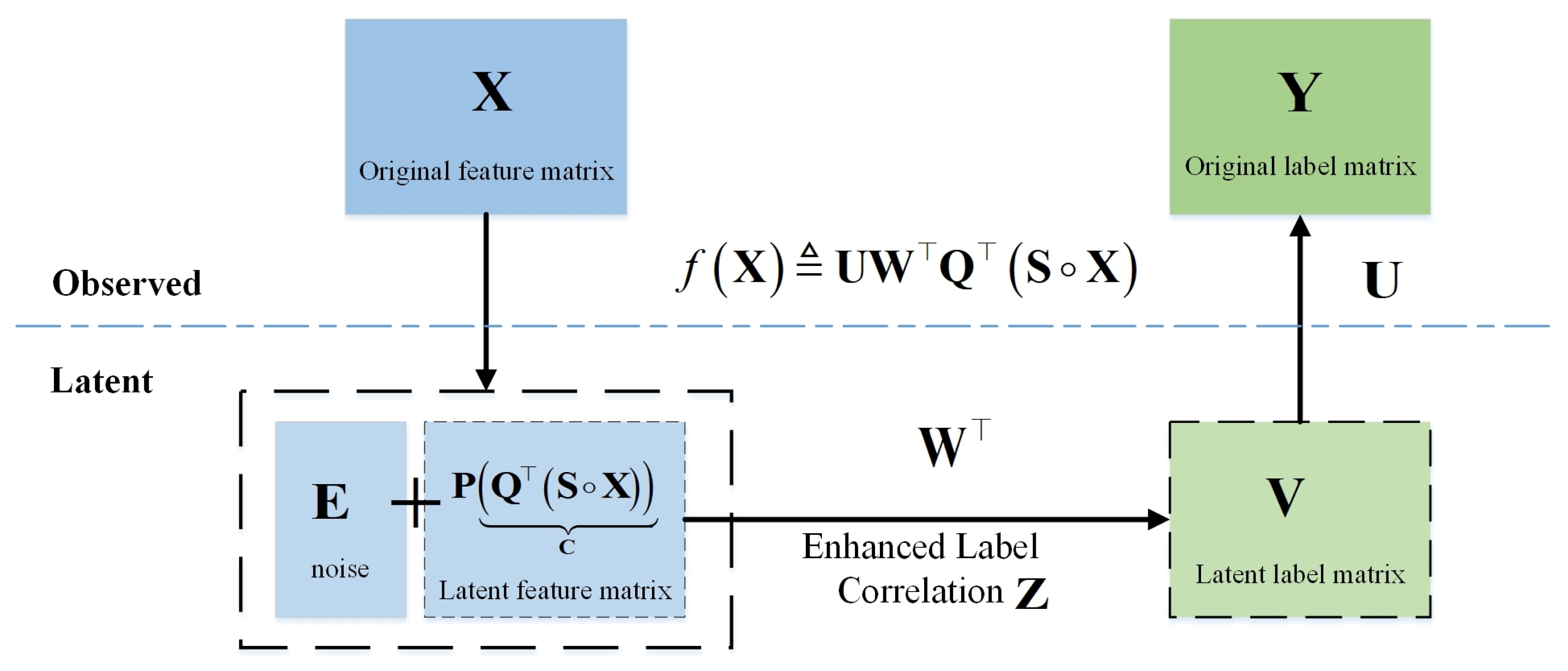
3.1. Proposed Model
3.1.1. Learning Latent Features
3.1.2. Learning Latent Labels
3.1.3. Global and Local Manifold Regularizer
3.1.4. Learning Label Correlations
3.1.5. Predicting Labels for Unseen Instances
3.2. Optimization
3.2.1. Solving (2)
3.2.2. Solving (9)
3.3. Computational Complexity Analysis
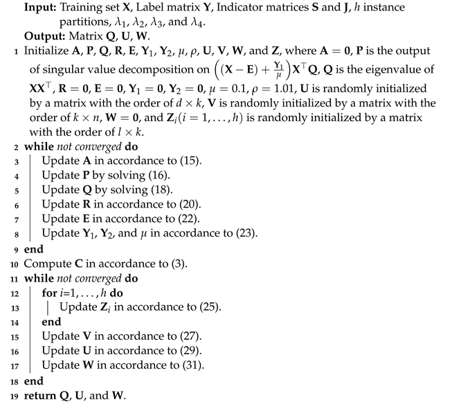
| Algorithm 1: RGLC |
 |
3.3.1. Complexity Analysis of Solving (2)
3.3.2. Complexity Analysis of Solving (9)
4. Results
4.1. Experimental Settings
- (1)
- Hamming Loss (abbreviated as Hl) evaluates the average difference between predictions and ground truth (see Formula (32)). The smaller the value of Hamming loss is, the better the performance of an algorithm becomes.where is the set symmetric difference and is the set cardinality.
- (2)
- Ranking Loss (abbreviated as Rkl) evaluates the fraction that an irrelevant label ranks before the relevant label in label predictions (see Formula (33)). The smaller the value of Ranking Loss is, the better the performance of an algorithm becomes.where denotes the ranking position in ascending order for the j-th label on the i-th instance. is the set cardinality.
- (3)
- One Error (abbreviated as Oe) evaluates whether the average fraction that the label ranks first in prediction is the irrelevant label (see Formula (34)). The smaller the value of One Error is, the better the performance of an algorithm becomes.where is equal to 1 if the condition holds, and it equals 0 otherwise. The operator denotes the ranking position in ascending order for the j-th label on the i-th instance.
- (4)
- Coverage (abbreviated as Cvg) evaluates the average fraction for inclusion of all ground-truth labels in the ranking of label predictions (see Formula 35). The smaller the value of Coverage is, the better the performance of an algorithm becomes.where denotes the ranking position in ascending order for the j-th label on the i-th instance.
- (5)
- Average Precision (abbreviated as Ap) evaluates the average precision of actually relevant labels ranking before a relevant label examined by label predictions (see Formula 36). The larger the value of Average Precision is, the better the performance of an algorithm becomes.where is the set cardinality.
- Multi-label learning with label-specific features (LIFT) http://palm.seu.edu.cn/zhangml/files/LIFT.rar (accessed on 21 January 2022) [54]: Generating cluster-based label-specific features for multi-label.
- Learning label-specific features (LLSF) https://jiunhwang.github.io/ (accessed on 21 January 2022) [55]: Learning label-specific features to promote multi-label classification performance.
- Multi-label twin support vector machine (MLTSVM) http://www.optimal-group.org/Resource/MLTSVM.html (accessed on 21 January 2022) [56]: Providing multi-label learning algorithm with twin support vector machine.
- Global and local label correlations (Glocal) http://www.lamda.nju.edu.cn/code_Glocal.ashx (accessed on 21 January 2022) [31]: Learning global and local correlation for multi-label.
- Hybrid noise-oriented multilabel learning (HNOML) [17]: A feature and label noise-resistance multi-label model.
- Manifold regularized discriminative feature selection for multi-label learning (MDFS) https://github.com/JiaZhang19/MDFS (accessed on 21 January 2022) [38]: Learning discriminative features via manifold regularization.
- Multilabel classification with group-based mapping (MCGM) https://github.com/JianghongMA/MC-GM (accessed on 21 January 2022) [43]: Group-based local correlation with local feature selection.
- Fast random k labelsets (fRAkEL) http://github.com/KKimura360/fast_RAkEL_matlab (accessed on 21 January 2022) [57]: A fast version of Random k-labelsets.
- RGLC: Proposed model. ,,, and are searched in . Cluster number and , as they have limited impacts on considered metrics.
4.2. Learning with Benchmarks
- From Table 2, we observe that for all six evaluation metrics, RGLC achieves the best performance or second-best performance in 66.67% (4/6) and 33.33% (2/6) cases according to the rank of “Avg rank” in terms of Hamming Loss, Ranking Loss, One Error, Coverage, Average Precision, and Micro F1. It is only inferior to LIFT and fRAkEL according to the rank of the value of “Avg rank” in Table 2 based on the evaluation metric Ranking Loss and One Error, respectively. Specifically, RGLC achieves 24 (33.33%) best (the number of values indicated in bold) and 18 (25%) second-best performances (the number of values indicated in underlined) on 72 observations (12 datasets × 6 metrics). In contrast, the second-best method is LIFT, which achieves 12 (16.67%) best and 18 (25%) second-best performances on 72 observations (12 datasets × 6 metrics).
- The Holm test in Table 4 shows that RGLC is statistically superior to other algorithms to varying degrees in all metrics, with the best performance in Average Precision (better than seven algorithms) and the worst performance in Ranking Loss (better than three algorithms). Concretely, RGLC significantly outperforms MCGM in terms of all metrics except Micro F1, significantly outperforms MLTSVM in terms of Hamming Loss, Ranking Loss, Coverage, and Average Precision, significantly outperforms Glocal in terms of Hamming Loss, Coverage, Average Precision, and Micro F1, significantly outperforms HNOML in terms of Hamming Loss, One Error, Average Precision, and Micro F1, significantly outperforms MDFS in terms of One Error, Coverage, Average Precision, and Micro F1, significantly outperforms fRAkEL in terms of Hamming Loss, Ranking Loss, Average Precision, and Micro F1, significantly outperforms LLSF in terms of Hamming Loss, One Error, and Average Precision and significantly outperforms LIFT in terms of Coverage.
4.3. Ablation Study
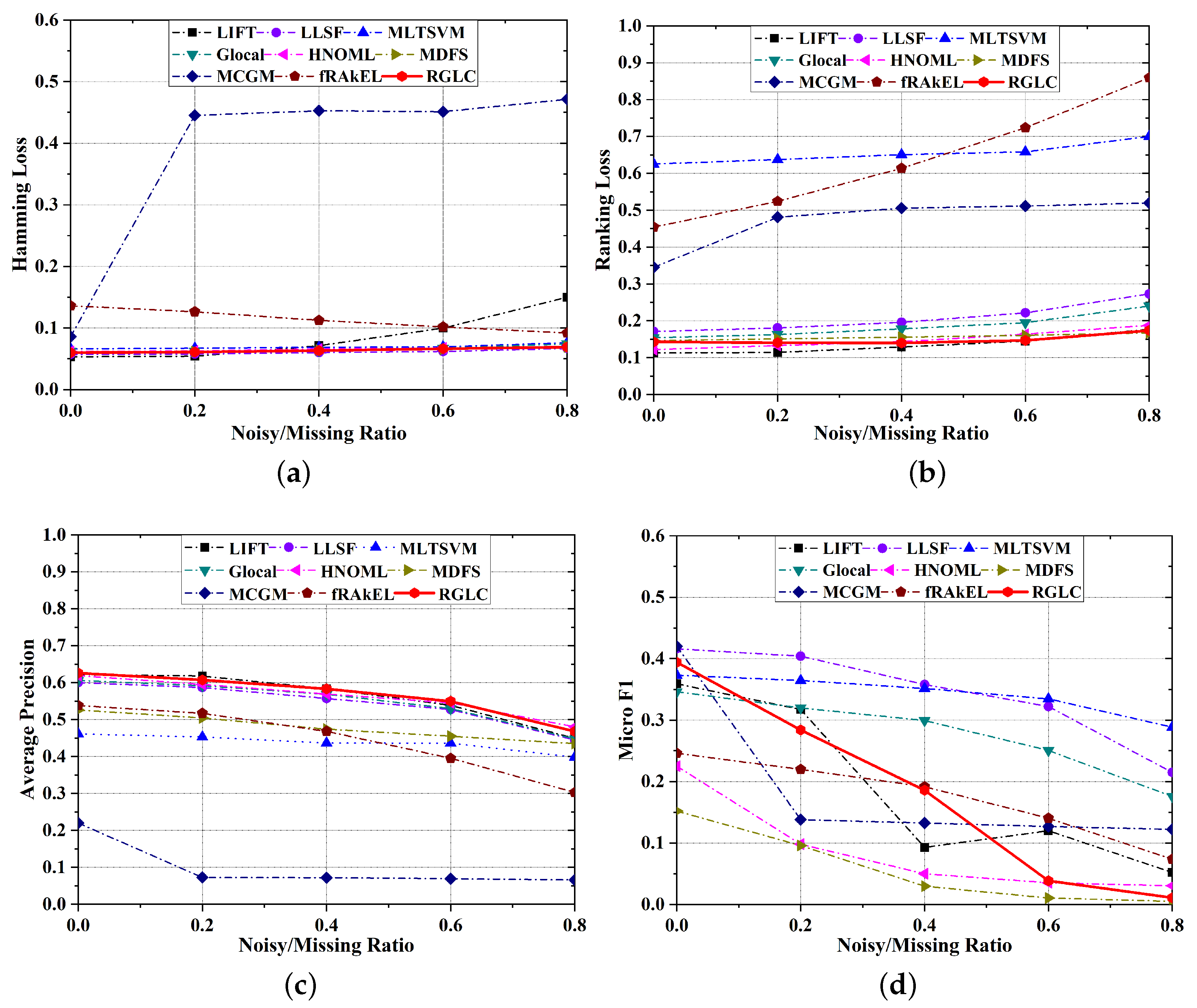
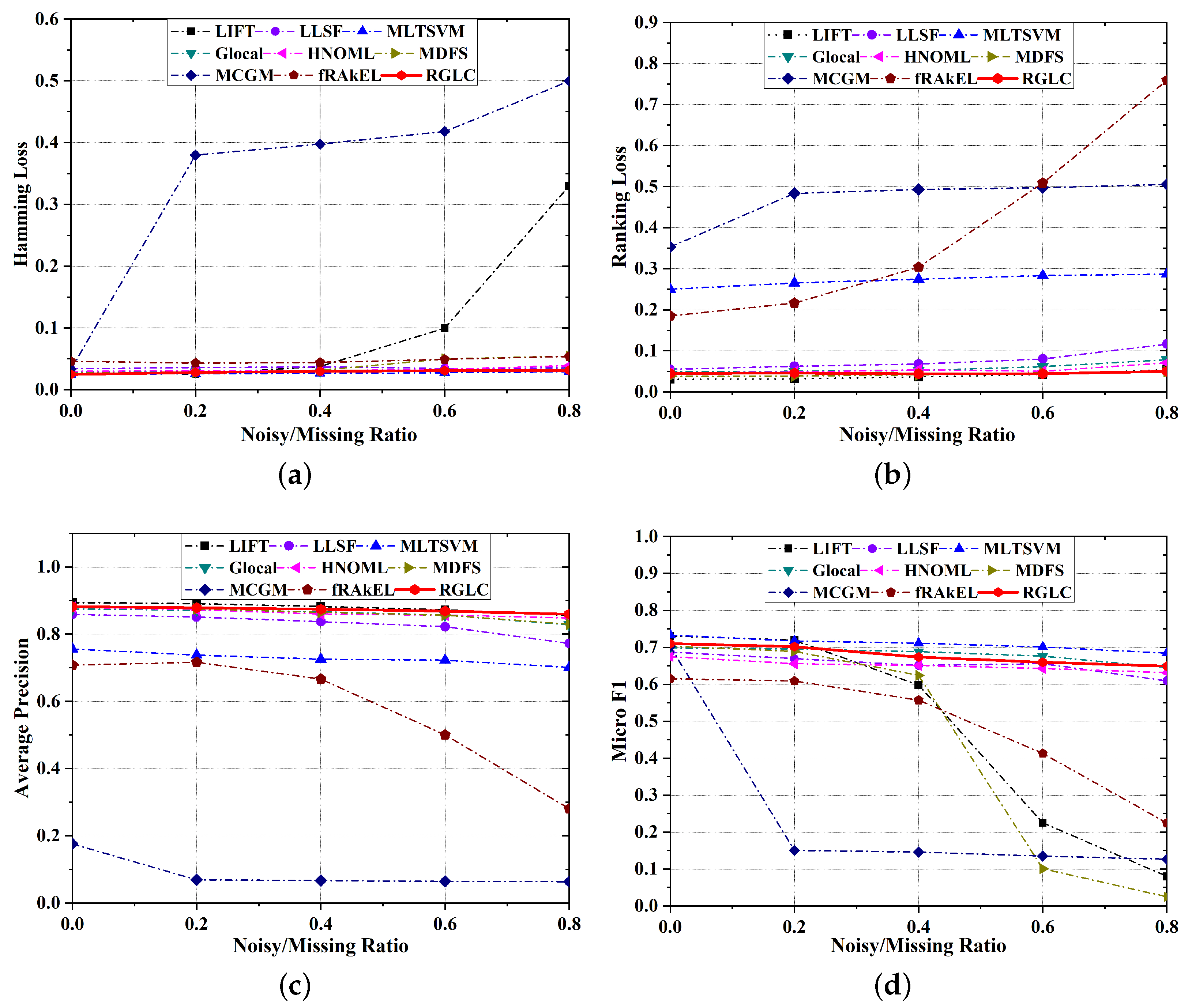
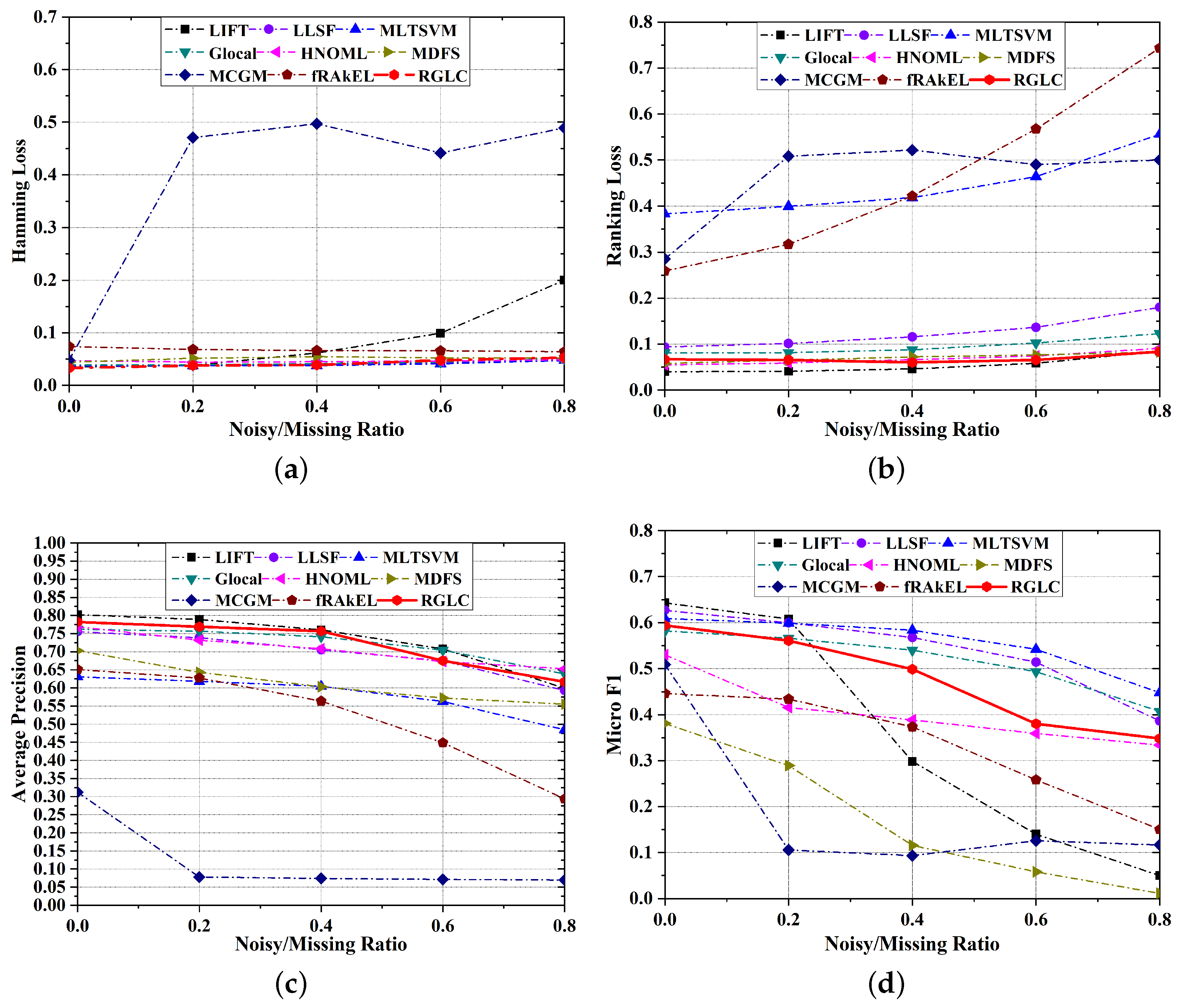
4.4. Learning with Noisy Features and Missing Labels
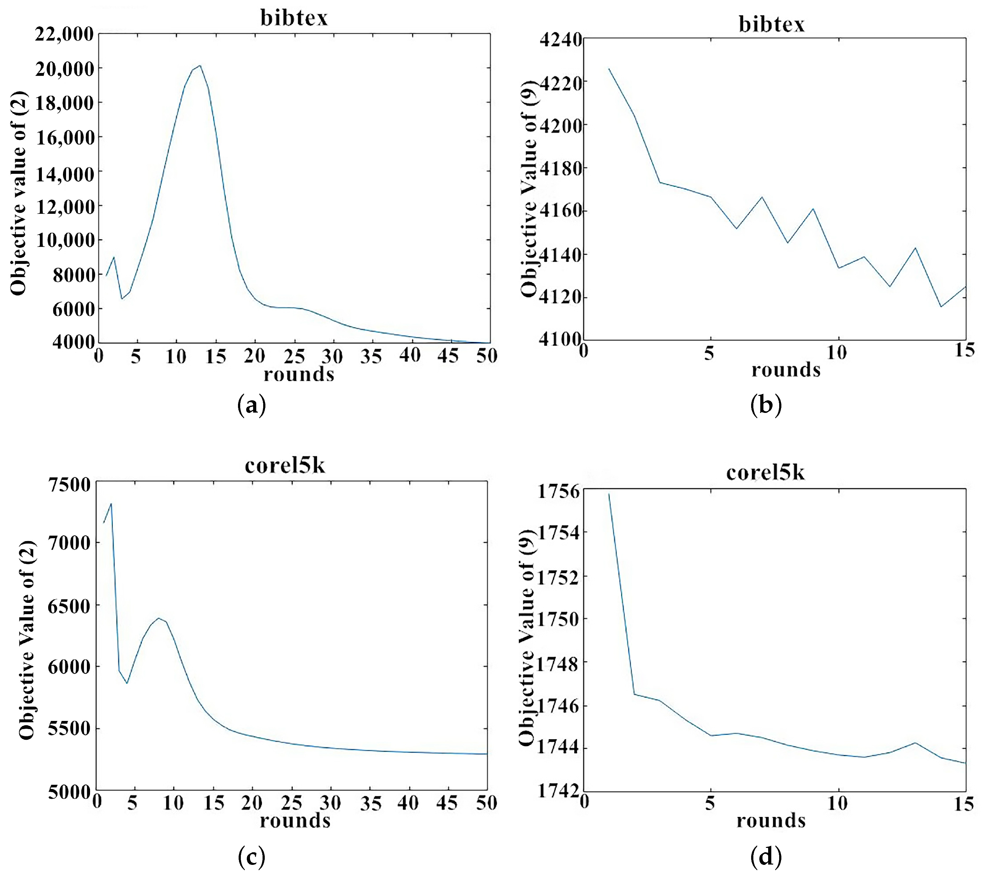
4.5. Convergence
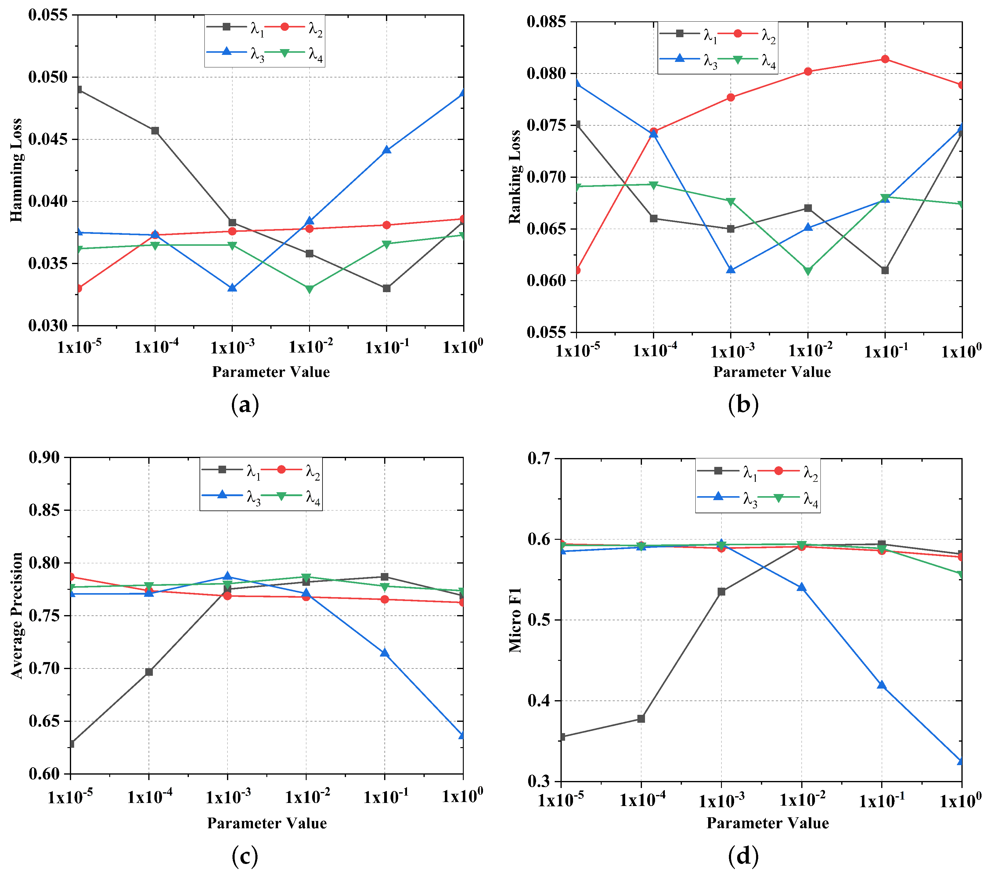
4.6. Sensitivity
5. Discussion
6. Conclusions
Author Contributions
Funding
Institutional Review Board Statement
Informed Consent Statement
Data Availability Statement
Acknowledgments
Conflicts of Interest
Correction Statement
References
- Zhang, M.L.; Zhou, Z.H. A review on multi-label learning algorithms. IEEE Trans. Knowl. Data Eng. 2014, 26, 1819–1837. [Google Scholar] [CrossRef]
- Gibaja, E.; Ventura, S. A tutorial on multilabel learning. ACM Comput. Surv. 2015, 47, 1–38. [Google Scholar] [CrossRef]
- Liu, W.W.; Shen, X.B.; Wang, H.B.; Tsang, I.W. The emerging trends of multi-label learning. IEEE Trans. Pattern Anal. Mach. Intell. 2021, in press. [Google Scholar] [CrossRef]
- Xu, W.H.; Li, W.T. Granular computing approach to two-way learning based on formal concept analysis in fuzzy datasets. IEEE Trans. Cybern. 2016, 46, 366–379. [Google Scholar] [CrossRef]
- Xu, W.H.; Yu, J.H. A novel approach to information fusion in multi-source datasets: A granular computing viewpoint. Inf. Sci. 2017, 378, 410–423. [Google Scholar] [CrossRef]
- Zhang, Y.J.; Miao, D.Q.; Zhang, Z.F.; Xu, J.F.; Luo, S. A three-way selective ensemble model for multi-label classification. Int. J. Approx. Reason. 2018, 103, 394–413. [Google Scholar] [CrossRef]
- Zhang, Y.J.; Miao, D.Q.; Pedrycz, W.; Zhao, T.N.; Xu, J.F.; Yu, Y. Granular structure-based incremental updating for multi-label classification. Knowl. Based Syst. 2020, 189, 105066:1–105066:15. [Google Scholar] [CrossRef]
- Zhang, Y.J.; Zhao, T.N.; Miao, D.Q.; Pedrycz, W. Granular multilabel batch active learning with pairwise label correlation. IEEE Trans. Syst. Man Cybern. Syst. 2022, 52, 3079–3091. [Google Scholar] [CrossRef]
- Yuan, K.H.; Xu, W.H.; Li, W.T.; Ding, W.P. An incremental learning mechanism for object classification based on progressive fuzzy three-way concept. Inf. Sci. 2022, 584, 127–147. [Google Scholar] [CrossRef]
- Xu, Y.H.; Yuan, K.H.; Li, W.T. Dynamic updating approximations of local generalized multigranulation neighborhood rough set. Appl. Intell. 2022, in press. [Google Scholar] [CrossRef]
- Guo, Y.M.; Chung, F.L.; Li, G.Z.; Wang, J.C.; Gee, J.C. Leveraging label-specific discriminant mapping features for multi-label learning. ACM Trans. Knowl. Discov. Data 2019, 13, 24:1–24:23. [Google Scholar] [CrossRef]
- Huang, D.; Cabral, R.; Torre, F.D.L. Robust regression. IEEE Trans. Pattern Anal. Mach. Intell. 2016, 38, 363–375. [Google Scholar] [CrossRef] [PubMed]
- Ma, J.H.; Zhang, H.J.; Chow, T.W.S. Multilabel classification with label-specific features and classifiers: A coarse- and fine-tuned framework. IEEE Trans. Cybern. 2021, 51, 1028–1042. [Google Scholar] [CrossRef] [PubMed]
- Zhang, J.; Lin, Y.D.; Jiang, M.; Li, S.Z.; Tang, Y.; Tan, K.C. Multi-label feature selection via global relevance and redundancy optimization. In Proceedings of the International Conference on Artificial Intelligence, Yokohama, Japan, 7–15 January 2020; pp. 2512–2518. [Google Scholar]
- Guo, B.L.; Hou, C.P.; Shan, J.C.; Yi, D.Y. Low rank multi-label classification with missing labels. In Proceedings of the International Conference on Pattern Recognition, Beijing, China, 21–24 August 2018; pp. 417–422. [Google Scholar]
- Sun, L.J.; Ye, P.; Lyu, G.Y.; Feng, S.H.; Dai, G.J.; Zhang, H. Weakly-supervised multi-label learning with noisy features and incomplete labels. Neurocomput. 2020, 413, 61–71. [Google Scholar] [CrossRef]
- Zhang, C.Q.; Yu, Z.W.; Fu, H.Z.; Zhu, P.F.; Chen, L.; Hu, Q.H. Hybrid noise-oriented multilabel learning. IEEE Trans. Cybern. 2020, 50, 2837–2850. [Google Scholar] [CrossRef] [PubMed]
- Lou, Q.D.; Deng, Z.H.; Choi, K.S.; Shen, H.B.; Wang, J.; Wang, S.T. Robust multi-label relief feature selection based on fuzzy margin co-optimization. IEEE Trans. Emerg. Top. Comput. Intell. 2022, 6, 387–398. [Google Scholar] [CrossRef]
- Fan, Y.L.; Liu, J.H.; Liu, P.Z.; Du, Y.Z.; Lan, W.Y.; Wu, S.X. Manifold learning with structured subspace for multi-label feature selection. Pattern Recogn. 2021, 120, 108169:1–108169:16. [Google Scholar] [CrossRef]
- Xu, M.; Li, Y.F.; Zhou, Z.H. Robust multi-label learning with pro loss. IEEE Trans. Knowl. Data Eng. 2020, 32, 1610–1624. [Google Scholar] [CrossRef]
- Braytee, A.; Liu, W.; Anaissi, A.; Kennedy, P.J. Correlated multi-label classification with incomplete label space and class imbalance. ACM Trans. Intell. Syst. Technol. 2019, 10, 56:1–56:26. [Google Scholar] [CrossRef]
- Dong, H.B.; Sun, J.; Sun, X.H. A multi-objective multi-label feature selection algorithm based on shapley value. Entropy 2021, 23, 1094. [Google Scholar] [CrossRef]
- Jain, H.; Prabhu, Y.; Varma, M. Extreme multi-label loss functions for recommendation, tagging, ranking & other missing label applications. In Proceedings of the ACM SIGKDD International Conference on Knowledge Discovery and Data Mining, San Francisco, CA, USA, 13–17 August 2016; pp. 935–944. [Google Scholar]
- Qarraei, M.; Schultheis, E.; Gupta, P.; Babbar, R. Convex surrogates for unbiased loss functions in extrem classification with missing labels. In Proceedings of the World Wide Web Conference, Ljubljana, Slovenia, 19–23 April 2021; pp. 3711–3720. [Google Scholar]
- Wydmuch, M.; Jasinska-Kobus, K.; Babbar, R.; Dembczynski, K. Propensity-scored probabilistic label trees. In Proceedings of the International ACM SIGIR Conference on Research and Development in Information Retrieval, Virtual Event, 11–15 July 2021; pp. 2252–2256. [Google Scholar]
- Chen, Z.J.; Hao, Z.F. A unified multi-label classification framework with supervised low-dimensional embedding. Neurocomputing 2016, 171, 1563–1575. [Google Scholar] [CrossRef]
- Chen, C.; Wang, H.B.; Liu, W.W.; Zhao, X.Y.; Hu, T.L.; Chen, G. Two-stage label embedding via neural factorization machine for multi-label classification. In Proceedings of the Association for the Advance in Artificial Intelligence, Hawaii, HI, USA, 27 December–1 January 2019; pp. 3304–3311. [Google Scholar]
- Wei, T.; Li, Y.F. Learning compact model for large-scale multi-label data. In Proceedings of the Association for the Advance in Artificial Intelligence, Hawaii, HI, USA, 27 December–1 January 2019; pp. 5385–5392. [Google Scholar]
- Huang, J.; Xu, L.C.; Wang, J.; Feng, L.; Yamanishi, K. Discovering latent class labels for multi-label learning. In Proceedings of the International Conference on Artificial Intelligence, Yokohama, Japan, 7–15 January 2020; pp. 3058–3064. [Google Scholar]
- Fang, X.Z.; Teng, S.H.; Lai, Z.H.; He, Z.S.; Xie, S.L.; Wong, W.K. Robust latent subspace learning for image classification. IEEE Trans. Neural Netw. Learn. Syst. 2018, 29, 2502–2515. [Google Scholar] [CrossRef] [PubMed]
- Zhu, Y.; Kwok, J.T.; Zhou, Z.H. Multi-label learning with global and local label correlation. IEEE Trans. Knowl. Data Eng. 2018, 30, 1081–1094. [Google Scholar] [CrossRef]
- Siblini, W.; Kuntz, P.; Meyer, F. A review on dimensionality reduction for multi-label classification. IEEE Trans. Knowl. Data Eng. 2021, 33, 839–857. [Google Scholar] [CrossRef]
- Yu, Z.B.; Zhang, M.L. Multi-label classification with label-specific feature generation: A wrapped approach. IEEE Trans. Pattern Anal. Mach. Intell. 2021, in press. [Google Scholar] [CrossRef]
- He, S.; Feng, L.; Li, L. Estimating latent relative labeling importances for multi-label learning. In Proceedings of the International Conference on Data Mining, Singapore, 17–20 November 2018; pp. 1013–1018. [Google Scholar]
- Zhong, Y.J.; Xu, C.; Du, B.; Zhang, L.F. Independent feature and label components for multi-label classification. In Proceedings of the International Conference on Data Mining, Singapore, 17–20 November 2018; pp. 827–836. [Google Scholar]
- Belkin, M.; Niyogi, P.; Sindhwani, V. Manifold regularization: A geometric framework for learning from labeled and unlabeled examples. J. Mach. Learn. Res. 2006, 7, 2399–2434. [Google Scholar]
- Cai, Z.L.; Zhu, W. Multi-label feature selection via feature manifold learning and sparsity regularization. Int. J. Mach. Learn. Cybern. 2018, 9, 1321–1334. [Google Scholar] [CrossRef]
- Zhang, J.; Luo, Z.M.; Li, C.D.; Zhou, C.E.; Li, S.Z. Manifold regularized discriminative feature selection for multi-label learning. Pattern Recogn. 2019, 95, 136–150. [Google Scholar] [CrossRef]
- Guan, Y.Y.; Li, X.M. Multilabel text classification with incomplete labels: A save generative model with label manifold regularization and confidence constraint. IEEE Multimedia 2020, 27, 38–47. [Google Scholar] [CrossRef]
- Feng, L.; Huang, J.; Shu, S.L.; An, B. Regularized matrix factorization for multilabel learning with missing labels. IEEE Trans. Cybern. 2020, in press. [Google Scholar] [CrossRef]
- Huang, S.J.; Zhou, Z.H. Multi-label learning by exploiting label correlation locally. In Proceedings of the Association for Advanced Artificial Intelligence, Toronto, ON, Canada, 22–26 July 2012; pp. 945–955. [Google Scholar]
- Jia, X.Y.; Zhu, S.S.; Li, W.W. Joint label-specific features and correlation information for multi-label learning. J. Comput. Sci. Technol. 2020, 35, 247–258. [Google Scholar] [CrossRef]
- Ma, J.H.; Chiu, B.C.Y.; Chow, T.W.S. Multilabel classification with group-based mapping: A framework with local feature selection and local label correlation. IEEE Trans. Cybern. 2020, in press. [Google Scholar] [CrossRef] [PubMed]
- Zhu, C.M.; Miao, D.Q.; Wang, Z.; Zhou, R.G.; Wei, L.; Zhang, X.F. Global and local multi-view multi-label learning. Neurocomputing 2020, 371, 67–77. [Google Scholar] [CrossRef]
- Sun, L.J.; Feng, S.H.; Liu, J.; Lyu, G.Y.; Lang, C.Y. Global-local label correlation for partial multi-label learning. IEEE Trans. Multimed. 2022, 24, 581–593. [Google Scholar] [CrossRef]
- Cai, X.; Ding, C.; Nie, F.; Huang, H. On the equivalent of low-rank linear regressions and linear discriminant analysis based regressions. In Proceedings of the ACM SIGKDD International Conference on Knowledge Discovery and Data Mining, Chicago, IL, USA, 11–14 August 2013; pp. 1124–1132. [Google Scholar]
- Sylvester, J. Sur l’equation en matrices px=xq. C. R. Acad. Sci. Paris 1884, 99, 67–71. [Google Scholar]
- Liu, G.C.; Lin, Z.C.; Yan, S.C.; Sun, J.; Yu, Y.; Ma, Y. Robust recovery of subspace structures by low-rank representation. IEEE Trans. Pattern Anal. Mach. Intell. 2013, 35, 171–184. [Google Scholar] [CrossRef]
- Boumal, N.; Mishra, B.; Absil, P.A.; Sepulchre, R. Manopt, a matlab toolbox for optimization on manifolds. J. Mach. Learn. Res. 2014, 15, 1455–1459. [Google Scholar]
- Tsoumakas, G.; Katakis, I.; Vlahavas, I. Mining Multi-label Data. In Data Mining and Knowledge Discovery Handbook; Maimon, O., Rokach, L., Eds.; Springer: Boston, MA, USA, 2009; pp. 667–685. [Google Scholar]
- Read, J.; Reutemann, P.; Pfahringer, B.; Holmes, G. Meka: A multi-label/multi-target extension to weka. J. Mach. Learn. Res. 2016, 17, 21:1–21:5. [Google Scholar]
- Zhang, Y.; Zhou, Z.H. Multilabel dimensionality reduction via dependence maximization. ACM Trans. Knowl. Disocv. Data 2010, 4, 14:1–14:21. [Google Scholar] [CrossRef]
- Schapire, R.E.; Singer, Y. BoosTexter: A boosting-based system for text categorization. Mach. Learn. 2000, 39, 135–168. [Google Scholar] [CrossRef]
- Zhang, M.L.; Wu, L. LIFT: Multi-label learning with label-specific features. IEEE Trans. Pattern Anal. Mach. Intell. 2015, 37, 107–120. [Google Scholar] [CrossRef] [PubMed]
- Huang, J.; Li, G.R.; Huang, Q.M.; Wu, X.D. Learning label-specific features and class-dependent labels for multi-label classification. IEEE Trans. Knowl. Data Eng. 2016, 28, 3309–3323. [Google Scholar] [CrossRef]
- Chen, W.J.; Shao, Y.H.; Li, C.N.; Deng, N.Y. MLTSVM: A novel twin support vector machine to multi-label learning. Pattern Recogn. 2016, 52, 61–74. [Google Scholar] [CrossRef]
- Kimura, K.; Kudo, M.; Sun, L.; Koujaku, S. Fast random k-labelsets for large-scale multi-label classification. In Proceedings of the International Conference on Pattern Recognition, Cancun, Mexico, 4–8 December 2016; pp. 438–443. [Google Scholar]
- Demsar, J. Statistical comparisons of classifier over multiple data sets. J. Mach. Learn. Res. 2006, 7, 1–30. [Google Scholar]

| Datasets | #n | #f | #q | #c | Domain |
|---|---|---|---|---|---|
| art | 5000 | 462 | 26 | 1.64 | text |
| bibtex | 7395 | 1836 | 159 | 2.402 | text |
| business | 5000 | 438 | 30 | 1.59 | text |
| corel5k | 5000 | 499 | 374 | 3.522 | image |
| enron | 1702 | 1001 | 53 | 3.378 | text |
| genbase | 662 | 1185 | 27 | 1.252 | biology |
| health | 5000 | 612 | 32 | 1.66 | text |
| languagelog | 1460 | 1004 | 75 | 1.18 | text |
| mediamill | 43907 | 120 | 101 | 4.376 | video |
| medical | 978 | 1449 | 45 | 1.245 | text |
| scene | 2407 | 294 | 6 | 1.074 | image |
| slashdot | 3782 | 1079 | 22 | 1.18 | text |
| Dataset | Hamming Loss (↓) | ||||||||
| LIFT | LLSF | MLTSVM | Glocal | HNOML | MDFS | MCGM | fRAkEL | RGLC | |
| art | 0.053 ± 0.001 | 0.057 ± 0.002 | 0.066 ± 0.001 | 0.062 ± 0.004 | 0.062 ± 0.001 | 0.061 ± 0.001 | 0.086 ± 0.006 | 0.136 ± 0.004 | 0.060 ± 0.002 |
| bibtex | 0.013 ± 0.001 | 0.015 ± 0.001 | 0.017 ± 0.001 | 0.014 ± 0.001 | 0.015 ± 0.001 | 0.013 ± 0.001 | 0.047 ± 0.006 | 0.046 ± 0.002 | 0.012 ± 0.001 |
| business | 0.028 ± 0.001 | 0.034 ± 0.002 | 0.025 ± 0.001 | 0.029 ± 0.001 | 0.030 ± 0.001 | 0.027 ± 0.002 | 0.033 ± 0.003 | 0.046 ± 0.002 | 0.025 ± 0.002 |
| corel5k | 0.010 ± 0.001 | 0.024 ± 0.002 | 0.015 ± 0.001 | 0.010 ± 0.001 | 0.009 ± 0.001 | 0.010 ± 0.001 | 0.201 ± 0.017 | 0.026 ± 0.001 | 0.009 ± 0.001 |
| enron | 0.109 ± 0.001 | 0.067 ± 0.001 | 0.062 ± 0.002 | 0.076 ± 0.006 | 0.056 ± 0.002 | 0.051 ± 0.002 | 0.062 ± 0.004 | 0.204 ± 0.008 | 0.057 ± 0.004 |
| genbase | 0.003 ± 0.001 | 0.001 ± 0.001 | 0.002 ± 0.001 | 0.003 ± 0.003 | 0.003 ± 0.003 | 0.005 ± 0.001 | 0.003 ± 0.001 | 0.002 ± 0.001 | 0.002 ± 0.004 |
| health | 0.035 ± 0.002 | 0.037 ± 0.001 | 0.037 ± 0.001 | 0.039 ± 0.002 | 0.047 ± 0.001 | 0.044 ± 0.001 | 0.048 ± 0.003 | 0.074 ± 0.004 | 0.033 ± 0.002 |
| languagelog | 0.016 ± 0.001 | 0.025 ± 0.001 | 0.029 ± 0.001 | 0.018 ± 0.001 | 0.016 ± 0.001 | 0.016 ± 0.001 | 0.028 ± 0.001 | 0.184 ± 0.007 | 0.015 ± 0.001 |
| mediamill | 0.030 ± 0.001 | 0.034 ± 0.001 | 0.033 ± 0.001 | 0.033 ± 0.001 | 0.033 ± 0.001 | 0.032 ± 0.001 | 0.035 ± 0.001 | 0.051 ± 0.005 | 0.032 ± 0.001 |
| medical | 0.013 ± 0.001 | 0.014 ± 0.001 | 0.014 ± 0.002 | 0.015 ± 0.001 | 0.014 ± 0.042 | 0.016 ± 0.016 | 0.016 ± 0.001 | 0.051 ± 0.005 | 0.011 ± 0.001 |
| scene | 0.094 ± 0.005 | 0.114 ± 0.002 | 0.143 ± 0.003 | 0.111 ± 0.006 | 0.147 ± 0.005 | 0.085 ± 0.008 | 0.119 ± 0.005 | 0.291 ± 0.020 | 0.089 ± 0.012 |
| slashdot | 0.017 ± 0.001 | 0.026 ± 0.001 | 0.212 ± 0.008 | 0.020 ± 0.001 | 0.020 ± 0.001 | 0.019 ± 0.001 | 0.029 ± 0.004 | 0.044 ± 0.002 | 0.016 ± 0.002 |
| Avg rank | 3.2500(2) | 5.0833(5) | 5.4583(7) | 5.1250(6) | 4.8750(4) | 3.8750(3) | 7.2917(8) | 8.2500(9) | 1.7917(1) |
| Dataset | Ranking Loss (↓) | ||||||||
| LIFT | LLSF | MLTSVM | Glocal | HNOML | MDFS | MCGM | fRAkEL | RGLC | |
| art | 0.113 ± 0.005 | 0.171 ± 0.006 | 0.625 ± 0.006 | 0.154 ± 0.016 | 0.122 ± 0.003 | 0.146 ± 0.002 | 0.345 ± 0.017 | 0.454 ± 0.015 | 0.143 ± 0.005 |
| bibtex | 0.078 ± 0.004 | 0.090 ± 0.002 | 0.659 ± 0.008 | 0.159 ± 0.005 | 0.136 ± 0.005 | 0.170 ± 0.006 | 0.252 ± 0.012 | 0.495 ± 0.005 | 0.074 ± 0.003 |
| business | 0.031 ± 0.002 | 0.055 ± 0.001 | 0.250 ± 0.004 | 0.049 ± 0.007 | 0.046 ± 0.004 | 0.038 ± 0.004 | 0.353 ± 0.021 | 0.185 ± 0.008 | 0.045 ± 0.003 |
| corel5k | 0.128 ± 0.003 | 0.190 ± 0.007 | 0.891 ± 0.002 | 0.148 ± 0.004 | 0.137 ± 0.002 | 0.132 ± 0.002 | 0.224 ± 0.012 | 0.812 ± 0.007 | 0.172 ± 0.003 |
| enron | 0.329 ± 0.006 | 0.189 ± 0.007 | 0.499 ± 0.012 | 0.132 ± 0.008 | 0.143 ± 0.007 | 0.088 ± 0.003 | 0.404 ± 0.014 | 0.424 ± 0.019 | 0.089 ± 0.011 |
| genbase | 0.003 ± 0.001 | 0.002 ± 0.002 | 0.006 ± 0.008 | 0.002 ± 0.001 | 0.002 ± 0.002 | 0.006 ± 0.002 | 0.031 ± 0.037 | 0.006 ± 0.006 | 0.003 ± 0.003 |
| health | 0.040 ± 0.003 | 0.094 ± 0.006 | 0.383 ± 0.012 | 0.081 ± 0.006 | 0.055 ± 0.005 | 0.058 ± 0.001 | 0.285 ± 0.012 | 0.259 ± 0.009 | 0.061 ± 0.002 |
| languagelog | 0.163 ± 0.007 | 0.232 ± 0.010 | 0.731 ± 0.014 | 0.193 ± 0.006 | 0.287 ± 0.016 | 0.159 ± 0.007 | 0.311 ± 0.021 | 0.546 ± 0.020 | 0.131 ± 0.010 |
| mediamill | 0.050 ± 0.001 | 0.047 ± 0.001 | 0.602 ± 0.005 | 0.056 ± 0.003 | 0.047 ± 0.001 | 0.060 ± 0.001 | 0.451 ± 0.008 | 0.132 ± 0.023 | 0.054 ± 0.001 |
| medical | 0.029 ± 0.006 | 0.035 ± 0.004 | 0.168 ± 0.018 | 0.201 ± 0.033 | 0.021 ± 0.059 | 0.043 ± 0.004 | 0.227 ± 0.023 | 0.131 ± 0.023 | 0.023 ± 0.005 |
| scene | 0.080 ± 0.007 | 0.113 ± 0.008 | 0.278 ± 0.009 | 0.096 ± 0.005 | 0.110 ± 0.010 | 0.076 ± 0.005 | 0.095 ± 0.010 | 0.243 ± 0.022 | 0.093 ± 0.008 |
| slashdot | 0.042 ± 0.003 | 0.035 ± 0.005 | 0.484 ± 0.022 | 0.069 ± 0.007 | 0.061 ± 0.008 | 0.050 ± 0.005 | 0.416 ± 0.035 | 0.144 ± 0.012 | 0.057 ± 0.004 |
| Avg rank | 2.4583(1) | 4.3750(5) | 8.5833(9) | 4.7500(6) | 3.3750(3) | 3.5000(4) | 7.5000(8) | 7.4167(7) | 3.0417(2) |
| Dataset | One Error (↓) | ||||||||
| LIFT | LLSF | MLTSVM | Glocal | HNOML | MDFS | MCGM | fRAkEL | RGLC | |
| art | 0.458 ± 0.026 | 0.471 ± 0.015 | 0.523 ± 0.007 | 0.468 ± 0.020 | 0.475 ± 0.011 | 0.610 ± 0.011 | 0.569 ± 0.069 | 0.303 ± 0.017 | 0.448 ± 0.006 |
| bibtex | 0.386 ± 0.009 | 0.358 ± 0.022 | 0.422 ± 0.010 | 0.528 ± 0.137 | 0.617 ± 0.007 | 0.532 ± 0.011 | 0.752 ± 0.025 | 0.194 ± 0.007 | 0.374 ± 0.011 |
| business | 0.106 ± 0.007 | 0.133 ± 0.008 | 0.092 ± 0.006 | 0.119 ± 0.009 | 0.126 ± 0.005 | 0.117 ± 0.010 | 0.660 ± 0.047 | 0.068 ± 0.007 | 0.116 ± 0.012 |
| corel5k | 0.690 ± 0.012 | 0.658 ± 0.010 | 0.745 ± 0.007 | 0.675 ± 0.021 | 0.727 ± 0.014 | 0.727 ± 0.017 | 0.722 ± 0.029 | 0.393 ± 0.012 | 0.644 ± 0.021 |
| enron | 0.637 ± 0.021 | 0.381 ± 0.027 | 0.139 ± 0.007 | 0.293 ± 0.037 | 0.300 ± 0.017 | 0.264 ± 0.010 | 0.760 ± 0.033 | 0.089 ± 0.018 | 0.230 ± 0.026 |
| genbase | 0.003 ± 0.000 | 0.003 ± 0.004 | 0.001 ± 0.001 | 0.002 ± 0.003 | 0.006 ± 0.003 | 0.017 ± 0.006 | 0.144 ± 0.060 | 0.002 ± 0.003 | 0.001 ± 0.003 |
| health | 0.238 ± 0.032 | 0.274 ± 0.010 | 0.236 ± 0.014 | 0.272 ± 0.015 | 0.293 ± 0.015 | 0.374 ± 0.017 | 0.476 ± 0.029 | 0.124 ± 0.006 | 0.254 ± 0.013 |
| languagelog | 0.690 ± 0.015 | 0.803 ± 0.025 | 0.679 ± 0.013 | 0.707 ± 0.026 | 0.773 ± 0.011 | 0.783 ± 0.025 | 0.852 ± 0.036 | 0.594 ± 0.033 | 0.676 ± 0.018 |
| mediamill | 0.137 ± 0.003 | 0.159 ± 0.004 | 0.134 ± 0.004 | 0.154 ± 0.003 | 0.191 ± 0.007 | 0.161 ± 0.003 | 0.960 ± 0.014 | 0.071 ± 0.012 | 0.151 ± 0.004 |
| medical | 0.163 ± 0.014 | 0.189 ± 0.017 | 0.113 ± 0.020 | 0.143 ± 0.032 | 0.154 ± 0.177 | 0.237 ± 0.025 | 0.510 ± 0.059 | 0.071 ± 0.012 | 0.142 ± 0.024 |
| scene | 0.240 ± 0.021 | 0.286 ± 0.015 | 0.177 ± 0.013 | 0.264 ± 0.011 | 0.292 ± 0.014 | 0.224 ± 0.019 | 0.208 ± 0.160 | 0.153 ± 0.024 | 0.258 ± 0.018 |
| slashdot | 0.091 ± 0.021 | 0.337 ± 0.023 | 0.086 ± 0.008 | 0.118 ± 0.013 | 0.332 ± 0.021 | 0.093 ± 0.019 | 0.790 ± 0.049 | 0.295 ± 0.010 | 0.092 ± 0.014 |
| Avg rank | 4.2083(4) | 5.9583(6) | 3.7917(3) | 4.9583(5) | 6.9583(8) | 6.4583(7) | 8.0000(9) | 1.6250(1) | 3.0417(2) |
| Dataset | Coverage (↓) | ||||||||
| LIFT | LLSF | MLTSVM | Glocal | HNOML | MDFS | MCGM | fRAkEL | RGLC | |
| art | 4.478 ± 0.181 | 0.245 ± 0.009 | 11.68 ± 0.129 | 5.903 ± 0.404 | 0.180 ± 0.005 | 5.299 ± 0.090 | 1131 ± 45.46 | 0.329 ± 0.013 | 0.211 ± 0.009 |
| bibtex | 22.10 ± 1.176 | 0.163 ± 0.005 | 0.501 ± 0.004 | 37.54 ± 1.114 | 0.214 ± 0.007 | 0.281 ± 0.012 | 1459 ± 32.58 | 0.416 ± 0.008 | 0.149 ± 0.004 |
| business | 1.949 ± 0.122 | 0.098 ± 0.003 | 9.307 ± 0.296 | 2.808 ± 0.289 | 0.087 ± 0.009 | 2.201 ± 0.199 | 951.9 ± 32.76 | 0.112 ± 0.005 | 0.086 ± 0.004 |
| corel5k | 113.6 ± 2.824 | 0.397 ± 0.014 | 340.2 ± 1.197 | 112.7 ± 1.269 | 0.320 ± 0.009 | 214.7 ± 8.136 | 73.21 ± 5.391 | 0.439 ± 0.007 | 0.384 ± 0.005 |
| enron | 33.91 ± 0.721 | 0.433 ± 0.027 | 30.89 ± 0.774 | 18.04 ± 0.872 | 0.356 ± 0.019 | 12.86 ± 0.408 | 328.3 ± 9.465 | 0.423 ± 0.030 | 0.240 ± 0.026 |
| genbase | 0.403 ± 0.054 | 0.010 ± 0.001 | 0.292 ± 0.167 | 0.352 ± 0.081 | 0.012 ± 0.003 | 0.565 ± 0.119 | 11.37 ± 5.464 | 0.016 ± 0.005 | 0.014 ± 0.004 |
| health | 2.549 ± 0.099 | 0.160 ± 0.006 | 11.91 ± 0.346 | 4.595 ± 0.350 | 0.106 ± 0.008 | 3.186 ± 0.076 | 829.8 ± 28.33 | 0.162 ± 0.008 | 0.124 ± 0.003 |
| languagelog | 13.14 ± 1.557 | 0.275 ± 0.001 | 30.79 ± 1.403 | 17.86 ± 0.308 | 0.293 ± 0.016 | 12.63 ± 0.770 | 163.4 ± 4.265 | 0.309 ± 0.014 | 0.143 ± 0.006 |
| mediamill | 17.63 ± 0.121 | 0.165 ± 0.001 | 57.99 ± 0.506 | 19.36 ± 0.229 | 0.163 ± 0.003 | 19.69 ± 0.314 | 0.861 ± 0.009 | 0.089 ± 0.019 | 0.151 ± 0.004 |
| medical | 1.811 ± 0.342 | 0.049 ± 0.004 | 4.648 ± 0.700 | 5.737 ± 0.828 | 0.033 ± 0.065 | 2.783 ± 0.347 | 78.17 ± 10.64 | 0.089 ± 0.019 | 0.037 ± 0.008 |
| scene | 0.482 ± 0.041 | 0.105 ± 0.007 | 0.887 ± 0.052 | 0.568 ± 0.033 | 0.108 ± 0.009 | 0.465 ± 0.025 | 444.7 ± 34.90 | 0.149 ± 0.014 | 0.089 ± 0.041 |
| slashdot | 0.857 ± 0.116 | 0.044 ± 0.005 | 9.644 ± 0.323 | 2.288 ± 0.208 | 0.056 ± 0.006 | 0.046 ± 0.004 | 742.9 ± 47.83 | 0.089 ± 0.009 | 0.055 ± 0.004 |
| Avg rank | 6.0833(6) | 2.5833(3) | 7.5833(8) | 6.9167(7) | 2.1667(2) | 5.7500(5) | 8.3333(9) | 3.8333(4) | 1.7500(1) |
| Dataset | Average Precision (↑) | ||||||||
| LIFT | LLSF | MLTSVM | Glocal | HNOML | MDFS | MCGM | fRAkEL | RGLC | |
| art | 0.622 ± 0.016 | 0.600 ± 0.009 | 0.461 ± 0.007 | 0.606 ± 0.021 | 0.619 ± 0.008 | 0.526 ± 0.006 | 0.220 ± 0.014 | 0.538 ± 0.015 | 0.626 ± 0.003 |
| bibtex | 0.563 ± 0.009 | 0.587 ± 0.014 | 0.324 ± 0.009 | 0.357 ± 0.010 | 0.360 ± 0.006 | 0.409 ± 0.007 | 0.164 ± 0.009 | 0.418 ± 0.008 | 0.589 ± 0.006 |
| business | 0.894 ± 0.004 | 0.859 ± 0.005 | 0.756 ± 0.003 | 0.875 ± 0.011 | 0.880 ± 0.005 | 0.882 ± 0.009 | 0.176 ± 0.022 | 0.708 ± 0.024 | 0.882 ± 0.007 |
| corel5k | 0.286 ± 0.007 | 0.251 ± 0.007 | 0.089 ± 0.003 | 0.273 ± 0.007 | 0.254 ± 0.004 | 0.254 ± 0.004 | 0.302 ± 0.043 | 0.160 ± 0.005 | 0.298 ± 0.008 |
| enron | 0.346 ± 0.014 | 0.556 ± 0.012 | 0.450 ± 0.011 | 0.642 ± 0.013 | 0.617 ± 0.008 | 0.654 ± 0.012 | 0.175 ± 0.004 | 0.427 ± 0.015 | 0.695 ± 0.018 |
| genbase | 0.995 ± 0.002 | 0.994 ± 0.004 | 0.989 ± 0.006 | 0.995 ± 0.003 | 0.993 ± 0.003 | 0.985 ± 0.005 | 0.892 ± 0.045 | 0.992 ± 0.007 | 0.996 ± 0.005 |
| health | 0.802 ± 0.019 | 0.755 ± 0.007 | 0.631 ± 0.008 | 0.762 ± 0.010 | 0.769 ± 0.011 | 0.703 ± 0.009 | 0.312 ± 0.019 | 0.651 ± 0.006 | 0.787 ± 0.005 |
| languagelog | 0.397 ± 0.027 | 0.266 ± 0.019 | 0.267 ± 0.011 | 0.387 ± 0.019 | 0.296 ± 0.033 | 0.319 ± 0.020 | 0.104 ± 0.006 | 0.183 ± 0.017 | 0.408 ± 0.013 |
| mediamill | 0.719 ± 0.002 | 0.695 ± 0.003 | 0.465 ± 0.004 | 0.692 ± 0.002 | NA | 0.686 ± 0.003 | 0.066 ± 0.001 | 0.764 ± 0.005 | 0.698 ± 0.001 |
| medical | 0.875 ± 0.012 | 0.864 ± 0.016 | 0.799 ± 0.024 | 0.766 ± 0.028 | 0.887 ± 0.151 | 0.805 ± 0.016 | 0.411 ± 0.048 | 0.764 ± 0.005 | 0.893 ± 0.015 |
| scene | 0.857 ± 0.013 | 0.821 ± 0.009 | 0.756 ± 0.005 | 0.840 ± 0.006 | 0.820 ± 0.010 | 0.867 ± 0.011 | 0.715 ± 0.027 | 0.797 ± 0.016 | 0.845 ± 0.011 |
| slashdot | 0.893 ± 0.025 | 0.664 ± 0.006 | 0.658 ± 0.014 | 0.875 ± 0.010 | 0.887 ± 0.010 | 0.882 ± 0.013 | 0.100 ± 0.014 | 0.592 ± 0.005 | 0.885 ± 0.012 |
| Avg rank | 2.5417(2) | 4.9583(6) | 7.2500(8) | 4.4583(3) | 4.5417(5) | 4.6667(4) | 8.2500(9) | 6.5000(7) | 1.8333(1) |
| Dataset | Micro F1(↑) | ||||||||
| LIFT | LLSF | MLTSVM | Glocal | HNOML | MDFS | MCGM | fRAkEL | RGLC | |
| art | 0.359 ± 0.010 | 0.416 ± 0.015 | 0.373 ± 0.004 | 0.346 ± 0.021 | 0.225 ± 0.007 | 0.152 ± 0.002 | 0.420 ± 0.014 | 0.246 ± 0.007 | 0.394 ± 0.015 |
| bibtex | 0.370 ± 0.013 | 0.487 ± 0.006 | 0.356 ± 0.003 | 0.239 ± 0.010 | 0.328 ± 0.002 | 0.273 ± 0.007 | 0.224 ± 0.021 | 0.181 ± 0.007 | 0.293 ± 0.006 |
| business | 0.731 ± 0.008 | 0.687 ± 0.013 | 0.733 ± 0.002 | 0.698 ± 0.005 | 0.675 ± 0.007 | 0.703 ± 0.014 | 0.702 ± 0.018 | 0.615 ± 0.014 | 0.710 ± 0.018 |
| corel5k | 0.073 ± 0.002 | 0.205 ± 0.041 | 0.119 ± 0.003 | 0.037 ± 0.009 | 0.006 ± 0.002 | 0.024 ± 0.001 | 0.194 ± 0.017 | 0.061 ± 0.004 | 0.123 ± 0.008 |
| enron | 0.241 ± 0.010 | 0.479 ± 0.016 | 0.501 ± 0.010 | 0.445 ± 0.021 | 0.483 ± 0.011 | 0.504 ± 0.026 | 0.552 ± 0.022 | 0.200 ± 0.012 | 0.521 ± 0.015 |
| genbase | 0.970 ± 0.014 | 0.991 ± 0.005 | 0.987 ± 0.007 | 0.980 ± 0.018 | 0.956 ± 0.036 | 0.938 ± 0.012 | 0.972 ± 0.009 | 0.975 ± 0.013 | 0.992 ± 0.031 |
| health | 0.643 ± 0.018 | 0.627 ± 0.004 | 0.609 ± 0.009 | 0.582 ± 0.015 | 0.201 ± 0.004 | 0.381 ± 0.023 | 0.509 ± 0.164 | 0.446 ± 0.018 | 0.594 ± 0.014 |
| languagelog | 0.172 ± 0.039 | 0.205 ± 0.023 | 0.221 ± 0.009 | 0.058 ± 0.010 | 0.074 ± 0.019 | 0.070 ± 0.023 | 0.263 ± 0.008 | 0.028 ± 0.005 | 0.133 ± 0.014 |
| mediamill | 0.556 ± 0.003 | 0.505 ± 0.003 | 0.474 ± 0.004 | 0.508 ± 0.003 | 0.465 ± 0.004 | 0.520 ± 0.004 | 0.514 ± 0.003 | 0.458 ± 0.034 | 0.533 ± 0.001 |
| medical | 0.753 ± 0.030 | 0.755 ± 0.029 | 0.759 ± 0.026 | 0.714 ± 0.024 | 0.708 ± 0.077 | 0.668 ± 0.019 | 0.698 ± 0.013 | 0.458 ± 0.034 | 0.798 ± 0.016 |
| scene | 0.760 ± 0.008 | 0.591 ± 0.026 | 0.674 ± 0.008 | 0.588 ± 0.009 | 0.602 ± 0.015 | 0.746 ± 0.024 | 0.617 ± 0.019 | 0.427 ± 0.037 | 0.653 ± 0.015 |
| slashdot | 0.772 ± 0.013 | 0.737 ± 0.012 | 0.643 ± 0.011 | 0.774 ± 0.017 | 0.745 ± 0.005 | 0.745 ± 0.020 | 0.682 ± 0.029 | 0.581 ± 0.012 | 0.778 ± 0.015 |
| Avg rank | 3.5833(2) | 3.8333(4) | 3.7500(3) | 5.8333(7) | 6.5417(8) | 6.0417(6) | 4.5000(5) | 8.1667(9) | 2.7500(1) |
| Metric | Critical Value | |
|---|---|---|
| Hamming Loss | 49.0944 | 2.0454 |
| Ranking Loss | 64.9111 | |
| One Error | 53.1111 | |
| Coverage | 78.3778 | |
| Average Precision | 55.3000 | |
| Micro F1 | 39.0833 |
| Hamming Loss | Ranking Loss | ||||||||
| j | algorithm | p | j | algorithm | p | ||||
| 2 | fRAEL | −5.7765 | 0.000000 | 0.006 | 2 | MLTSVM | −4.9566 | 0.000000 | 0.006 |
| 3 | MCGM | −4.9194 | 0.000001 | 0.007 | 3 | MCGM | −3.9876 | 0.000067 | 0.007 |
| 4 | MLTSVM | −3.2796 | 0.001040 | 0.008 | 4 | fRAEL | −3.9131 | 0.000091 | 0.008 |
| 5 | Glocal | −2.9814 | 0.002869 | 0.010 | 5 | Glocal | −1.5279 | 0.126537 | 0.010 |
| 6 | LLSF | −2.9442 | 0.003238 | 0.013 | 6 | LLSF | −1.1925 | 0.233065 | 0.013 |
| 7 | HNOML | −2.7578 | 0.005819 | 0.017 | 7 | MDFS | −0.4099 | 0.681879 | 0.017 |
| 8 | MDFS | −1.8634 | 0.062407 | 0.025 | 8 | HNOML | −0.2981 | 0.765627 | 0.025 |
| 9 | LIFT | −1.3044 | 0.192106 | 0.050 | 9 | LIFT | 0.5218 | 1.000000 | 0.050 |
| One Error | Coverage | ||||||||
| j | algorithm | p | j | algorithm | p | ||||
| 2 | MCGM | −4.4348 | 0.000009 | 0.006 | 2 | MCGM | −5.8883 | 0.000000 | 0.006 |
| 3 | HNOML | −3.5031 | 0.000460 | 0.007 | 3 | MLTSVM | −5.2175 | 0.000000 | 0.007 |
| 4 | MDFS | −3.0559 | 0.002244 | 0.008 | 4 | Glocal | −4.6212 | 0.000004 | 0.018 |
| 5 | LLSF | −2.6087 | 0.009089 | 0.010 | 5 | LIFT | −3.8759 | 0.000106 | 0.010 |
| 6 | Glocal | −1.7143 | 0.086474 | 0.013 | 6 | MDFS | −3.5778 | 0.000347 | 0.013 |
| 7 | LIFT | −1.0434 | 0.296763 | 0.017 | 7 | fRAkEL | −1.8634 | 0.062407 | 0.017 |
| 8 | MLTSVM | −0.6708 | 0.502348 | 0.025 | 8 | LLSF | −0.7454 | 0.456057 | 0.025 |
| 9 | fRAkEL | 1.2671 | 1.000000 | 0.050 | 9 | HNOML | −0.3727 | 0.709388 | 0.050 |
| Average Precision | Micro F1 | ||||||||
| j | algorithm | p | j | algorithm | p | ||||
| 2 | MCGM | −5.7392 | 0.000000 | 0.006 | 2 | fRAEL | −4.8448 | 0.000001 | 0.006 |
| 3 | MLTSVM | −4.8448 | 0.000001 | 0.007 | 3 | HNOML | −3.3914 | 0.000695 | 0.007 |
| 4 | fRAEL | −4.1740 | 0.000030 | 0.008 | 4 | MDFS | −2.9442 | 0.003238 | 0.008 |
| 5 | LLSF | −2.7951 | 0.005189 | 0.010 | 5 | Glocal | −2.7578 | 0.005819 | 0.010 |
| 6 | MDFS | −2.5342 | 0.011270 | 0.013 | 6 | MCGM | −1.5652 | 0.117525 | 0.013 |
| 7 | HNOML | −2.4224 | 0.015418 | 0.017 | 7 | LIFT | −0.9690 | 0.332564 | 0.017 |
| 8 | Glocal | −2.3479 | 0.018881 | 0.025 | 8 | MLTSVM | −0.8944 | 0.371093 | 0.025 |
| 9 | LIFT | −0.6336 | 0.526373 | 0.050 | 9 | LLSF | −0.7454 | 0.456057 | 0.050 |
| Dataset | Hamming Loss (↓) | Dataset | Ranking Loss (↓) | ||||||||
| RGLC | RGLC-LF | RGLC-LL | RGLC-GC | RGLC-LC | RGLC | RGLC-LF | RGLC-LL | RGLC-GC | RGLC-LC | ||
| art | 0.060(2) | 0.062(5) | 0.061(4) | 0.060(2) | 0.060(2) | art | 0.143(1) | 0.156(5) | 0.153(4) | 0.146(3) | 0.144(2) |
| bibtex | 0.012(1) | 0.014(5) | 0.013(3) | 0.013(3) | 0.013(3) | bibtex | 0.074(1) | 0.131(5) | 0.085(2.5) | 0.085(2.5) | 0.089(4) |
| business | 0.025(1) | 0.028(4) | 0.028(4) | 0.027(2) | 0.028(4) | business | 0.045(1) | 0.051(5) | 0.050(4) | 0.046(2) | 0.047(3) |
| corel5k | 0.009(2) | 0.009(2) | 0.010(4.5) | 0.009(2) | 0.010(4.5) | corel5k | 0.172(2) | 0.161(1) | 0.199(5) | 0.177(3) | 0.195(4) |
| enron | 0.057(1) | 0.073(5) | 0.072(4) | 0.071(3) | 0.068(2) | enron | 0.089(1) | 0.128(5) | 0.125(3.5) | 0.122(2) | 0.125(3.5) |
| genbase | 0.002(3) | 0.001(1) | 0.003(5) | 0.002(3) | 0.002(3) | genbase | 0.003(4) | 0.002(1.5) | 0.003(4) | 0.002(1.5) | 0.003(4) |
| health | 0.033(1) | 0.039(5) | 0.037(3.5) | 0.036(2) | 0.037(3.5) | health | 0.061(1) | 0.081(5) | 0.075(4) | 0.069(2) | 0.070(3) |
| languagelog | 0.015(1) | 0.018(5) | 0.017(4) | 0.016(2.5) | 0.016(2.5) | languagelog | 0.131(1) | 0.226(5) | 0.178(3) | 0.187(4) | 0.179(2) |
| mediamill | 0.032(1) | 0.033(3.5) | 0.033(3.5) | 0.033(3.5) | 0.033(3.5) | mediamill | 0.054(1) | 0.056(2.5) | 0.056(2.5) | 0.057(4) | 0.058(5) |
| medical | 0.011(2) | 0.018(5) | 0.011(2) | 0.011(2) | 0.012(4) | medical | 0.023(3.5) | 0.039(5) | 0.019(1) | 0.022(2) | 0.023(3.5) |
| scene | 0.089(1) | 0.121(5) | 0.116(4) | 0.110(2.5) | 0.110(2.5) | scene | 0.093(1) | 0.102(5) | 0.095(3.5) | 0.094(2) | 0.095(3.5) |
| slashdot | 0.016(1) | 0.022(5) | 0.017(3) | 0.017(3) | 0.017(3) | slashdot | 0.057(1) | 0.070(5) | 0.069(4) | 0.068(3) | 0.067(2) |
| Avg. Rank | 1.417(1) | 4.208(5) | 3.708(4) | 2.542(2) | 3.125(3) | Avg Rank | 1.542(1) | 4.167(5) | 3.417(4) | 2.583(2) | 3.292(3) |
| Dataset | One Error (↓) | Dataset | Coverage (↓) | ||||||||
| RGLC | RGLC-LF | RGLC-LL | RGLC-GC | RGLC-LC | RGLC | RGLC-LF | RGLC-LL | RGLC-GC | RGLC-LC | ||
| art | 0.448(1) | 0.468(5) | 0.458(2) | 0.460(3) | 0.459(4) | art | 0.211(1) | 5.96(5) | 0.225(4) | 0.215(3) | 0.214(2) |
| bibtex | 0.374(2) | 0.491(5) | 0.364(1) | 0.380(3) | 0.383(4) | bibtex | 0.149(1) | 33.15(5) | 0.163(3) | 0.161(2) | 0.169(4) |
| business | 0.116(1) | 0.122(4.5) | 0.122(4.5) | 0.118(2.5) | 0.118(2.5) | business | 0.086(1) | 2.864(5) | 0.094(4) | 0.087(2) | 0.088(3) |
| corel5k | 0.644(1) | 0.647(2) | 0.652(5) | 0.650(3) | 0.651(4) | corel5k | 0.384(1) | 129.5(5) | 0.445(4) | 0.405(2) | 0.439(3) |
| enron | 0.230(1) | 0.283(5) | 0.264(2) | 0.279(4) | 0.266(3) | enron | 0.240(1) | 17.44(5) | 0.314(3) | 0.310(2) | 0.319(4) |
| genbase | 0.001(1) | 0.006(3) | 0.003(3.5) | 0.002(2) | 0.003(3.5) | genbase | 0.015(4) | 0.348(5) | 0.014(2.5) | 0.012(1) | 0.014(2.5) |
| health | 0.254(1) | 0.272(5) | 0.262(4) | 0.255(2) | 0.256(3) | health | 0.143(4) | 4.595(5) | 0.135(3) | 0.127(1) | 0.129(2) |
| languagelog | 0.676(2) | 0.743(5) | 0.665(1) | 0.689(4) | 0.678(3) | languagelog | 0.143(1) | 20.58(5) | 0.188(2) | 0.198(4) | 0.193(3) |
| mediamill | 0.151(1) | 0.153(2) | 0.169(5) | 0.167(3.5) | 0.167(3.5) | mediamill | 0.151(1) | 19.28(5) | 0.180(2) | 0.185(3) | 0.187(4) |
| medical | 0.142(1) | 0.162(5) | 0.155(4) | 0.147(2) | 0.149(3) | medical | 0.037(3) | 2.496(5) | 0.031(1) | 0.038(4) | 0.036(2) |
| scene | 0.258(1) | 0.281(5) | 0.269(3) | 0.276(4) | 0.268(2) | scene | 0.089(1) | 0.599(5) | 0.091(2) | 0.092(3) | 0.093(4) |
| slashdot | 0.092(1) | 0.116(5) | 0.108(4) | 0.104(2) | 0.105(3) | slashdot | 0.055(1) | 2.317(5) | 0.065(4) | 0.064(3) | 0.062(2) |
| Avg. Rank | 1.167(1) | 4.292(5) | 3.250(4) | 2.917(2) | 3.208(3) | Avg Rank | 1.667(1) | 5.000(5) | 2.875(3) | 2.500(2) | 2.958(4) |
| Dataset | Average Precision (↑) | Dataset | Micro F1 (↑) | ||||||||
| RGLC | RGLC-LF | RGLC-LL | RGLC-GC | RGLC-LC | RGLC | RGLC-LF | RGLC-LL | RGLC-GC | RGLC-LC | ||
| art | 0.626(1) | 0.606(5) | 0.614(3.5) | 0.614(3.5) | 0.618(2) | art | 0.394(1) | 0.349(5) | 0.353(2) | 0.338(3.5) | 0.338(3.5) |
| bibtex | 0.589(1) | 0.433(5) | 0.580(2) | 0.573(3) | 0.570(4) | bibtex | 0.293(4) | 0.254(5) | 0.348(1) | 0.305(3) | 0.334(2) |
| business | 0.882(1) | 0.873(4.5) | 0.873(4.5) | 0.878(2) | 0.876(3) | business | 0.710(2) | 0.707(4.5) | 0.708(3) | 0.714(1) | 0.707(4.5) |
| corel5k | 0.298(1) | 0.283(5) | 0.289(4) | 0.292(2) | 0.291(3) | corel5k | 0.123(2) | 0.056(4) | 0.188(1) | 0.037(5) | 0.090(3) |
| enron | 0.695(1) | 0.648(5) | 0.662(2) | 0.658(4) | 0.661(3) | enron | 0.521(1) | 0.457(5) | 0.464(4) | 0.467(3) | 0.480(2) |
| genbase | 0.996(1.5) | 0.994(4) | 0.995(3) | 0.996(1.5) | 0.993(5) | genbase | 0.991(1) | 0.985(2) | 0.972(5) | 0.976(3.5) | 0.976(3.5) |
| health | 0.787(1) | 0.762(5) | 0.772(4) | 0.779(2) | 0.778(3) | health | 0.594(2) | 0.582(5) | 0.596(1) | 0.593(3) | 0.590(4) |
| languagelog | 0.408(2) | 0.346(5) | 0.416(1) | 0.401(4) | 0.405(3) | languagelog | 0.133(2) | 0.134(1) | 0.127(3) | 0.089(4) | 0.071(5) |
| mediamill | 0.698(1) | 0.693(2) | 0.680(5) | 0.683(3) | 0.681(4) | mediamill | 0.533(1) | 0.509(2) | 0.490(5) | 0.493(3) | 0.492(4) |
| medical | 0.893(1) | 0.862(5) | 0.886(4) | 0.887(2.5) | 0.887(2.5) | medical | 0.798(1) | 0.703(5) | 0.794(2.5) | 0.794(2.5) | 0.779(4) |
| scence | 0.845(1) | 0.829(5) | 0.839(2.5) | 0.836(4) | 0.839(2.5) | scene | 0.653(1) | 0.543(5) | 0.581(4) | 0.628(2) | 0.622(3) |
| slashdot | 0.885(1) | 0.867(5) | 0.875(2.5) | 0.875(2.5) | 0.878(4) | slashdot | 0.778(1) | 0.773(2) | 0.767(5) | 0.769(4) | 0.772(3) |
| Avg. Rank | 1.208(1) | 4.625(5) | 3.167(3) | 2.833(2) | 3.250(4) | Avg Rank | 1.583(1) | 3.792(5) | 3.042(2) | 3.125(3) | 3.458(4) |
| Dataset | Algorithms | ||||||||
|---|---|---|---|---|---|---|---|---|---|
| LIFT | LLSF | MLTSVM | Glocal | HNOML | MDFS | MCGM | fRAkEL | RGLC | |
| art | 162.4(9) | 0.337(2) | 87.41(8) | 26.34(3) | 50.16(5) | 56.06(6) | 65.80(7) | 0.317(1) | 27.97(4) |
| bibtex | 1033(9) | 5.432(2) | 630.5(8) | 349.3(5) | 370.6(6) | 253.8(4) | 246.4(3) | 1.658(1) | 482.9(7) |
| business | 201.1(9) | 0.420(2) | 99.48(8) | 24.24(3) | 45.95(5) | 46.66(6) | 77.64(7) | 0.168(1) | 30.04(4) |
| corel5k | 466.2(9) | 5.469(2) | 425.9(8) | 106.3(5) | 83.31(4) | 133.7(6) | 160.7(7) | 4.298(1) | 72.57(3) |
| enron | 22.02(7) | 0.559(1) | 5.107(4) | 35.04(8) | 8.611(5) | 5.007(3) | 10.77(6) | 0.608(2) | 81.94(9) |
| genbase | 2.463(6) | 0.546(2) | 1.089(4) | 15.73(8) | 2.783(7) | 0.620(3) | 2.007(5) | 0.293(1) | 46.28(9) |
| health | 538.0(9) | 0.647(2) | 94.44(8) | 21.69(3) | 64.63(6) | 50.77(4) | 72.75(7) | 0.284(1) | 51.47(5) |
| mediamill | 1555(9) | 9.209(1) | 454.1(8) | 154.9(3) | 438.9(7) | 435.5(6) | 224.3(5) | 12.60(2) | 198.8(4) |
| medical | 8.858(7) | 1.313(2) | 2.958(4) | 30.12(9) | 5.576(5) | 1.552(3) | 7.183(6) | 0.347(1) | 29.87(8) |
| scene | 11.94(9) | 0.143(1) | 2.131(3) | 4.158(5) | 7.412(8) | 5.917(7) | 5.451(6) | 0.906(2) | 4.143(4) |
| slashdot | 36.72(7) | 0.459(1) | 15.55(3) | 15.10(2) | 40.08(8) | 21.69(5) | 17.29(4) | 24.45(6) | 59.77(9) |
| Total&Rank | 7.50(9) | 1.50(1) | 5.50(7) | 4.50(4) | 5.50(7) | 4.42(3) | 5.25(5) | 1.58(2) | 5.50(7) |
Publisher’s Note: MDPI stays neutral with regard to jurisdictional claims in published maps and institutional affiliations. |
© 2022 by the authors. Licensee MDPI, Basel, Switzerland. This article is an open access article distributed under the terms and conditions of the Creative Commons Attribution (CC BY) license (https://creativecommons.org/licenses/by/4.0/).
Share and Cite
Zhao, T.; Zhang, Y.; Pedrycz, W. Robust Multi-Label Classification with Enhanced Global and Local Label Correlation. Mathematics 2022, 10, 1871. https://doi.org/10.3390/math10111871
Zhao T, Zhang Y, Pedrycz W. Robust Multi-Label Classification with Enhanced Global and Local Label Correlation. Mathematics. 2022; 10(11):1871. https://doi.org/10.3390/math10111871
Chicago/Turabian StyleZhao, Tianna, Yuanjian Zhang, and Witold Pedrycz. 2022. "Robust Multi-Label Classification with Enhanced Global and Local Label Correlation" Mathematics 10, no. 11: 1871. https://doi.org/10.3390/math10111871
APA StyleZhao, T., Zhang, Y., & Pedrycz, W. (2022). Robust Multi-Label Classification with Enhanced Global and Local Label Correlation. Mathematics, 10(11), 1871. https://doi.org/10.3390/math10111871