Magnetorheological Fluid of High-Speed Unsteady Flow in a Narrow-Long Gap: An Unsteady Numerical Model and Analysis

Abstract

To investigate the unsteady flow field generated by magnetorheological (MR) fluid of a high-speed unsteady laminar boundary layer flow in a narrow-long gap of the magnetorheological absorber (MRA), a new unsteady numerical model is proposed. The gap has magnetic-field-activated and inactivated regions, with MR fluid flowing as bi-viscous (non-Newtonian) and Newtonian fluid. The unsteady flow field is described by the unsteady incompressible governing partial differential equation (PDE) and initial-boundary conditions with the moving boundary. The space-time solution domain is discretized using the finite difference method, and the governing PDE is transformed into implicit partial difference equations. The volume flow rate function is constructed to solve numerical solutions of pressure gradient and fluid velocity based on mass conservation, the continuity equation, and the bisection method. The accuracy of unsteady numerical model is validated by the experiment data. The results show that the fluid acceleration profiles along the gap’s height are non-uniform distribution. Further, the volume flow rate and excitation current has a significant impact on the dynamic distribution of fluid velocity profiles, and the moving boundary makes the flow field asymmetric about the central plane. Furthermore, as the transition stress increases, the thickness of the pre-yield region in the activated region increases. There is also a transition flow phenomenon in the activated region as the volume flow rate increases. Finally, the unsteady numerical model has good stability and convergence.

1. Introduction

The partial differential equation (PDE) is a useful tool in engineering and science for describing a variety of physical phenomena such as fluid flow, heat transfer, and diffusion [1,2,3]. In comparison to ordinary differential equations, PDE could fully consider the variation of variables with respect to space and time, allowing it to more accurately reflect the variation law of the physical phenomena discussed above. The development of supercomputers in recent years has made it possible to solve PDE using numerical methods, allowing researchers to investigate some complex physical phenomena. In this paper, a new unsteady numerical model is proposed to investigate the unsteady flow field generated by magnetorheological (MR) fluid as Newtonian fluid and bi-viscous (non-Newtonian) fluid of the high-speed laminar boundary layer unsteady flow in a narrow-long gap of the magnetorheological absorber (MRA) under impact. In particular, in comparison to Newtonian fluid, there are fewer numerical studies on non-Newtonian fluid’s unsteady flow. In addition, the nonlinear rheological behavior of non-Newtonian fluid gives rise to additional difficulties for modeling and solving, and the velocity profiles in the gap will be more complex and interesting.

The rheological properties of MR fluid can be controlled with the magnetic field, making it one of the research hotspots for smart materials. The shear rate-variation range is wide when MR fluid flows at high-speeds in the gap, and MR fluid has pre-yield and post-yield regions as the shear rate increases. Because the viscosity of the pre-yield region is greater than that of the post-yield region, the bi-viscous model [4,5,6], which is used in the current numerical model, is a commonly used rheology model. The MRA is a semi-active vibration isolation and buffer device that works with MR fluid as its working medium. Inside the MRA, there is a narrow-long annular gap with magnetic-field-activated and inactivated regions. The field-dependent pressure drop in the activated region can be controlled by adjusting the applied current to change the magnetic field intensity of the activated region, thereby controlling the mechanical properties of the MRA. The MRA has been widely used in vehicle suspension [7,8], landing gear [9,10], and vibration isolation [11,12] research over the last few decades because of its advantages of continuous and adjustable hydraulic resistance, rapid response, and low power consumption. The MR fluid in the gap is a fully developed unsteady laminar flow for the above applications. As a result, developing a mathematical model to solve the unsteady flow field and predict the dynamic mechanical characteristics of the MRA is critical for its development. There are currently quasi-static and unsteady models for analyzing the flow of MR fluid in the gap, with the main difference being whether or not the inertia term is taken into account. The quasi-static model’s governing equation is an ordinary differential equation without a time-dependent inertia term, and fluid viscosity causes the pressure drop along the gap [13,14,15]. The quasi-static model is widely used in the structural design and performance evaluation of the MRA because flow inertia is not taken into account. Under high-frequency and -impact conditions, the fluid acceleration in the gap increases. The flow inertia, in addition to the fluid viscosity, will have a significant impact on the pressure drop in the gap. However, research on the impact of fluid flow inertia on the pressure drop has received little attention.

Zhang et al. [16] conducted a sinusoidal excitation test to investigate the MR fluid squeeze flow and observed that the flow inertia increased significantly as the frequency was increased. The uniform flow inertia was used to analyze the inertia force. Chen et al. [17] developed a mathematical model that included flow inertia and used average fluid acceleration to investigate the effect of flow inertia on the pressure drop in the gap under sinusoidal excitation. Nguyen et al. [18] used the Laplace transform method to solve the governing PDE and obtain the pressure drop of unsteady flow electrorheological fluid in the gap. Additionally, the sinusoidal excitation test showed that the unsteady state behavior was obvious at high frequencies. To solve the pressure gradient of MR fluid in unsteady flow in the gap under sinusoidal oscillation, Zolfagharian et al. [19] developed an unsteady analytical model. It is found that the flow inertia increased as the oscillation frequency increased, according to the parametric study of the quasi-static and unsteady models. Notably, the aforementioned sinusoidal excitation is repetitive motion, and the volume flow in gap changes regularly. However, the volume flow rate in the gap of the MRA changes dramatically under impact, and the changes in fluid velocity profiles and pressure drop are more complicated. Wang et al. [20] tested the dynamic characteristics of the MRA using a pendulum impact test and found that the peak acceleration in the initial impact stage was up to approximately 400 g. Zhang et al. [21] tested the dynamic response of electrorheological energy absorbers under drop-weight impact and investigated the flow inertia in the gap by using average fluid acceleration. Mao et al. [22,23] studied the dynamic behavior of the MRA under high-speed impact conditions, and the flow inertia in the gap was approximately analyzed by average fluid acceleration. When analyzing the influence of fluid flow inertia on pressure drop, some of the above literature approximates the fluid acceleration to be evenly distributed along the height of the gap to simplify the analysis. Then, the pressure drop in the gap can be simplified by superimposing the pressure drop generated by the quasi-static model and the uniform flow inertia [16,17,22,23]. In fact, the velocity of MR fluid unsteady flow in the gap changes dynamically with time and space, which can be described by the unsteady governing PDE. Thus, by solving the numerical solution of the unsteady governing PDE, the unsteady flow field in the gap can be analyzed more precisely. In order to solve the unsteady governing PDE, a new unsteady numerical model based on the finite difference method is proposed in this paper. The pressure drop caused by the dynamic coupling of fluid viscosity and non-uniform flow inertia is investigated, and the actual non-uniform fluid acceleration profiles are presented as well as the space-time dynamic distribution of MR fluid velocity of unsteady flow in the gap.

The proposed unsteady numerical model is unique and worthwhile according to the aforementioned literature and to the best of the authors’ knowledge. The rest of the paper is organized as follows. In Section 2, we cover the problem’s background and analyze the magnetic flux density along the gap. In Section 3, we introduce the constitutive model of MR fluid and identify the model parameters. In Section 4, we establish an unsteady numerical model. The governing PDE and the initial-boundary conditions with moving boundary are utilized to model the unsteady flow field in the gap. The space-time solution domain is discretized using the finite difference method, and the governing PDE is transformed into implicit partial difference equations. Then, based on mass conservation, the continuity equation, and the bisection method, the volume flow rate function is constructed to solve the numerical solutions of fluid velocity and pressure gradient. In Section 5, the experimental setup is described as well as the test results. In Section 6, the numerical simulation calculation is introduced. In Section 7, the accuracy of unsteady numerical model is validated by the test data. In addition, the effects of the volume flow rate, moving boundary, and transition stress on velocity distribution are discussed, and the space-time dynamic distribution of MR fluid velocity is presented. The transition flow phenomenon of the activated region is also presented, and non-uniform acceleration profiles in the gap are revealed. Finally, the impact of mesh density on the results of unsteady numerical model is discussed. In Section 8, the main conclusions are drawn.

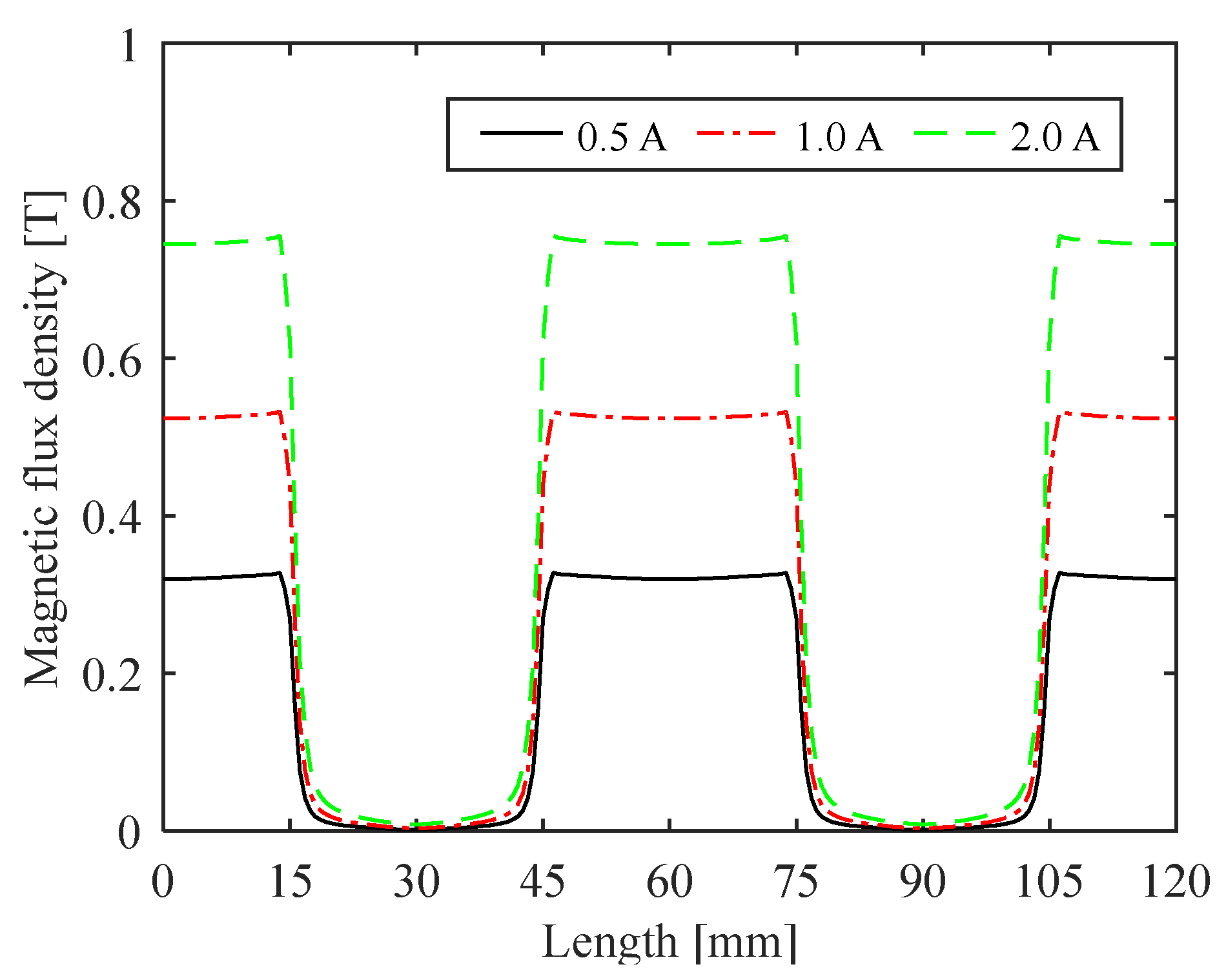
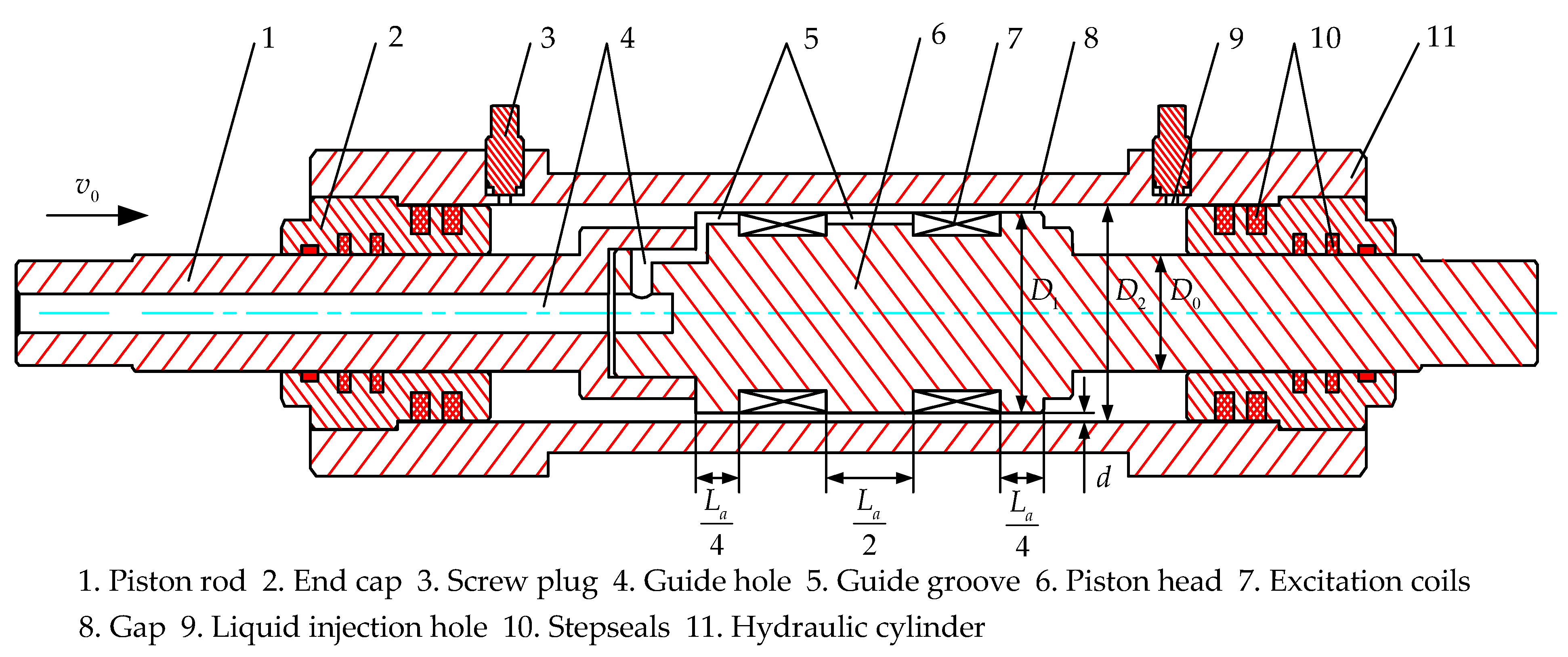
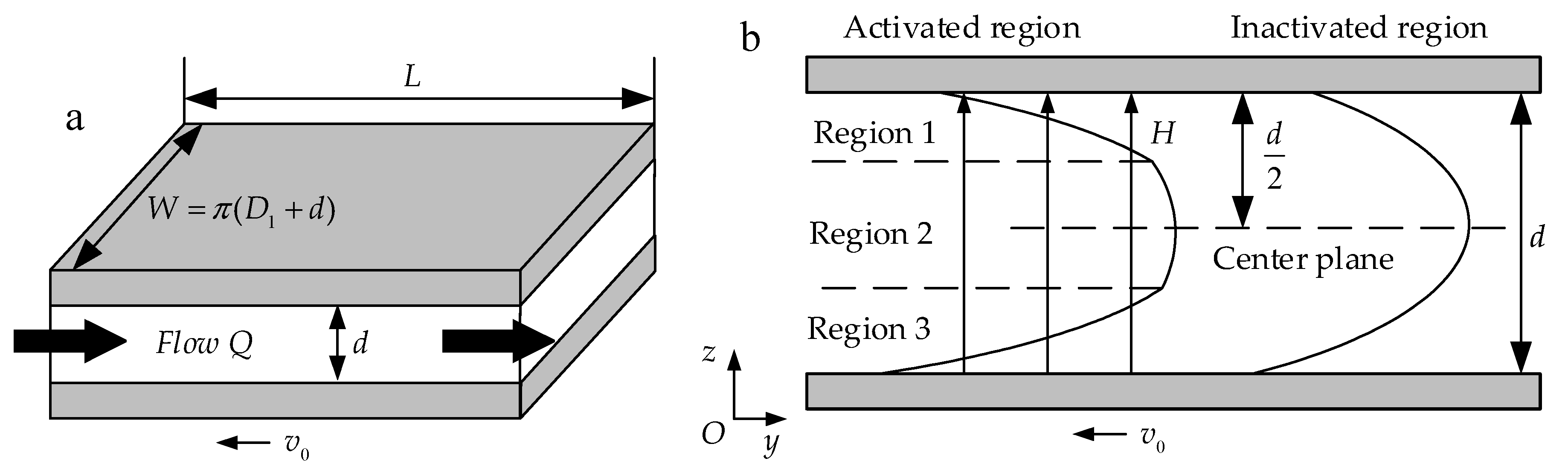
2. Structure and Magnetic Field Analysis of the MRA

Figure 1 shows the two-dimensional (2D) structure schematic of the MRA with the single cylinder and double-ended piston rods, which includes the piston rod, end cap, hydraulic cylinder, piston head, and other components. Because the diameters of the left and right piston rods are same, the volume of the inner chamber remains constant as the piston rods move. The piston head divides the hydraulic cylinder into two chambers. The excitation coils have a two-stage series connection and are reverse-wound. The external wires of the excitation coils lead to the outside of the MRA through the guide hole and guide groove. The stepseals are used to provide a dynamic seal between the piston rods and end caps. The liquid injection hole on the hydraulic cylinder is used to inject MR fluid into the inner chamber.

The piston rods move to the right relative to the hydraulic cylinder when the left piston rod is subjected to the axial impact force. The MR fluid in the right chamber is squeezed and then flows into the left chamber through the annular gap between the piston head and hydraulic cylinder. Adjusting the excitation currents changes the magnetic flux density in the annular gap, enabling the rheological behavior of the MR fluid to be adjusted and the MRA force output to be controlled. Figure 1 shows the structural parameters of the MRA, which will be used in the subsequent theoretical analysis.

The ANSYS software simulates the magnetic circuit, which is composed of the piston head, excitation coils, and hydraulic cylinder. The magnetic flux density along the annular gap for different excitation currents is shown in Figure 2. The magnetic flux density in the corresponding regions of excitation coils, known as the inactivated regions, is approximately zero. The magnetic flux density in other regions, known as the activated regions, increases with the increase in excitation currents and is uniformly distributed. The least squares method is used to fit polynomial data in simulations as follows:

$$B=2.324\times {10}^{-2}{I}^3-2.159\times {10}^{-1}{I}^2+7.124\times {10}^{-1}I,$$

(1)

where B is the magnetic flux density, and I is the excitation current.

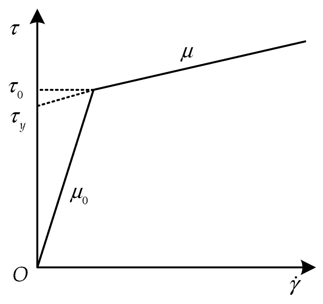
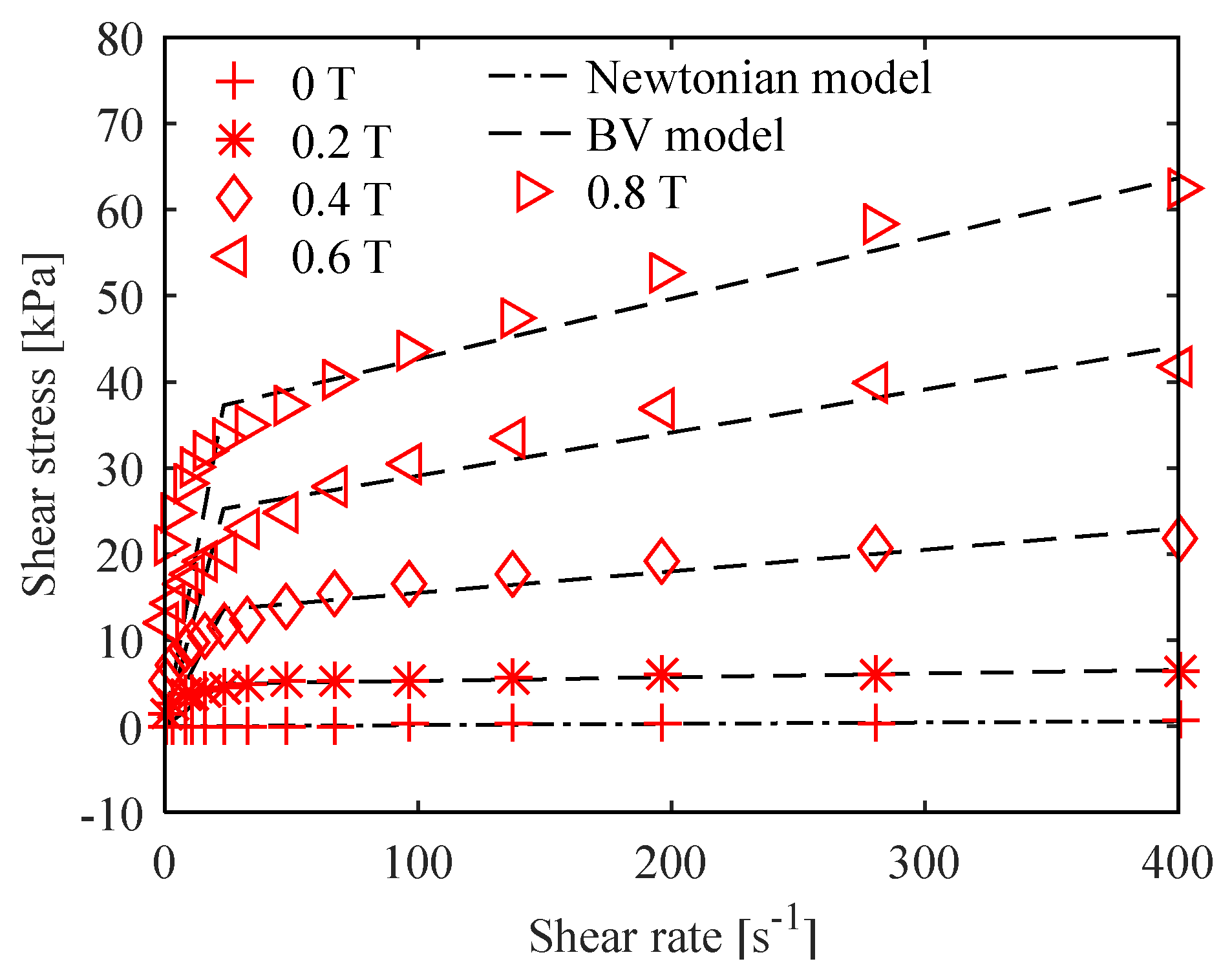
3. MR Fluid Characteristics

The MR fluid is a stable suspension of ferromagnetic particles dispersed uniformly in a base liquid. It is a Newtonian fluid with good fluidity in the absence of a magnetic field, for which the Newtonian fluid model can be described by

$$\tau ={\mu }_n\dot{\mathit{\gamma }},$$

(2)

where $\tau$ is the shear stress, ${\mu }_n$ is the fluid viscosity, and $\dot{\mathit{\gamma }}$ is the shear rate.

In the presence of a magnetic field, the MR fluid has the pre-yield and post-yield regions with increasing the shear rate, and the transition from the pre-yield region to the post-yield region occurs once the shear stress exceeds the transition stress. Because the pre-yield region’s viscosity is higher than that of the post-yield region, the bi-viscous model is utilized to describe the rheological behavior of the MR fluid, as shown in Figure 3. The constitutive model is given as

$$\tau =\{\begin{array}{l}{\mu }_0\dot{\mathit{\gamma }}, \left|\tau \right|\le {\tau }_0,\\ \mu \dot{\mathit{\gamma }}+(1-\frac{\mu }{{\mu }_0}){\tau }_0\mathrm{sgn}(\dot{\mathit{\gamma }}), \left|\tau \right|>{\tau }_0,\end{array}$$

(3)

where ${\tau }_0$ is the transition stress; ${\mu }_0$ and $\mu$ are the pre-yield region and post-yield region viscosity, respectively. ${\tau }_y$ is the yield shear stress in Figure 3.

The rheological behavior of the MR fluid changes with increasing the magnetic flux density, which is tested by the Anton Paar rheometer (MCR301). The parameters of the constitutive model are identified using the particle swarm optimization algorithm for various magnetic flux density, and the results are shown in Figure 4. The least squares method is used to fit the relationship between magnetic flux density and transition stress as follows:

$${\tau }_0=-4.98\times {10}^4{B}^3+8.91\times {10}^4{B}^2+6.65\times {10}^{3}B.$$

(4)

4. Unsteady Numerical Model

Because the gap’s height is much smaller than the diameter of the piston head, the narrow-long annular gap geometry is approximated using the parallel plates gap model [18,19] as shown in Figure 5a. The upper parallel plate is fixed, while the lower parallel plate moves, and the volume flow rate in the gap changes unsteadily. Therefore, the unsteady governing PDE and initial-boundary conditions with a moving boundary are used to model the high-speed incompressible unsteady laminar boundary layer flow of MR fluid in the gap, which is an initial-boundary value problem. Figure 5b depicts the typical velocity profiles of the activated and inactivated regions in the parallel plates. The gap’s height is $d$, the coordinate axis $y$ points from the gap’s inlet to the outlet, and the coordinate axis $z$ is normal to the parallel plates. Regions 1 and 3 have higher shear stress than the transition stress in the activated region, which is called the post-yield region; region 2 has lower shear stress than the transition stress, which is called the pre-yield region.

The unsteady governing PDE obtained from the incompressible Navier–Stokes equations as follows:

$$\{\begin{array}{l}\rho \frac{\partial u(z,t)}{\partial t}=-\frac{\partial p(t)}{\partial y}+\frac{\partial \tau (z,t)}{\partial z},\hfill \\ \nabla \cdot u(z,t)=0,\hfill \end{array}$$

(5)

where $\rho$ is the MR fluid density, and $t$ is the time variable. $u(z,t)$ is the fluid velocity, which varies with the gap coordinate $z$ and time variable $t$. $\partial u(z,t)/\partial t$ is the inertia term (fluid acceleration), which has non-uniform distribution along the coordinate $z$. $\partial p(t)/\partial y$ is the unsteady source term (pressure gradient), which changes uniformly along the coordinate $y$. $\partial \tau (z,t)/\partial z$ is the viscous term.

The shear rate of the MR fluid in the gap is denoted by

$$\dot{\mathit{\gamma }}=\frac{\partial u(z,t)}{\partial z}.$$

(6)

The piston head and the MR fluid in the gap are both stationary initially. The upper parallel plate remains stationary during the impact process, while the bottom parallel plate moves at the same velocity as the piston head. Accordingly, the MR fluid velocity in the gap’s initial value and Dirichlet boundary conditions are given as

$$\{\begin{array}{l}u(z,0)=0, 0\le z\le 1,\hfill \\ u(0,t)=-v_0, t>0,\hfill \\ u(d,t)=0, t>0.\hfill \end{array}$$

(7)

Here, $v_0$ is the velocity of the moving boundary (or piston head). Because the moving boundary moves in the opposite direction of the MR fluid’s general flow, its velocity is negative during impact. The above initial-boundary conditions are the definite condition of Equation (5).

The 2D solution domain is composed of space coordinate $z$ and time coordinate $t$, which are discretized by fixed space step $\Delta z$ and time step $\Delta t$ as shown in Figure 6. The gap’s height is divided into $J$ equal halves, i.e., $d=J\Delta z$. The intersections of vertical and horizontal lines are mesh points, and their coordinates are denoted by

$$\{\begin{array}{l}{z}_j=j\Delta z, j=0,1,2\cdots ,J,\hfill \\ t_n=n\Delta t, n=0,1,2\cdots .\hfill \end{array}$$

(8)

Here, any mesh point $(j,n)$ represents the point $(j\Delta x,n\Delta t)$ of the solution domain, and its velocity is denoted by $u_j^n=u(j\Delta x,n\Delta t)$. Moreover, the continuous 2D solution domain is discretized.

The governing PDE (5) is transformed into the partial difference equations of implicit type based on the finite difference method [24]. First, the forward difference in time is applied to replace the first-order partial derivative term of velocity with respect to time when $\Delta t\to 0$

$${(\frac{\partial u}{\partial t})}_j^n=\frac{u_j^{n+1}-u_j^n}{\Delta t}.$$

(9)

Then, the centered difference in space is applied to replace the second-order partial derivative term of velocity with respect to space when $\Delta z^2\to 0$:

$${(\frac{\partial u^2}{{\partial }^{2}z})}_j^n=\frac{u_{j+1}^n-2u_j^n+u_{j-1}^n}{\Delta z^2}.$$

(10)

The Taylor series can be used to prove the compatibility of Equations (9) and (10) when $\Delta t,\Delta z^2\to 0$.

Rearranging Equation (5) in term of Equations (2), (6), (9) and (10) yields the implicit partial difference equation in the whole inactivated region:

$$u_j^{n+1}=r_n{u}_{j+1}^n+(1-2r_n)u_j^n+r_n{u}_{j-1}^n-G\Delta p_0^{n+1},$$

(11)

where $r_n=\frac{\Delta t{\mu }_n}{\rho {(\Delta z)}^2}$, $G=\Delta t/\rho$, $\Delta p_0^{n+1}$ is the pressure gradient of the inactivated region at time $(n+1)\Delta t$.

By definition, ${\dot{\mathit{\gamma }}}_j^n=(u_{j+1}^n-u_j^n)/\Delta z$, and ${\dot{\mathit{\gamma }}}_{j-1}^n=(u_j^n-u_{j-1}^n)/\Delta z$, which are the shear rates calculated using the velocity of adjacent mesh points at time $n\Delta t$ because the activated region includes both the pre-yield and post-yield regions, and the thickness of the pre-yield region dynamic varies depending on the volume flow rate and excitation current. Thus, in the whole activated region, rearranging Equation (5) in term of Equations (3), (6), (9) and (10) yields the four types of the implicit partial difference equations:

• In the post-yield region, $\left|{\mu }_0{\dot{\mathit{\gamma }}}_j^n\right|>{\tau }_0\&\left|{\mu }_0{\dot{\mathit{\gamma }}}_{j-1}^n\right|>{\tau }_0$

  $$u_j^{n+1}=r{u}_{j+1}^n+(1-2r)u_j^n+r{u}_{j-1}^n+\frac{\Delta t{\tau }_0}{\Delta z\rho }(1-\frac{\mu }{{\mu }_0})[\mathrm{sgn}({\dot{\mathit{\gamma }}}_j^n)-\mathrm{sgn}({\dot{\mathit{\gamma }}}_{j-1}^n)]-G\Delta p^{n+1} ,$$

  (12)

  where $r=\frac{\Delta t\mu }{\Delta z^2\rho }$, $\Delta p^{n+1}$ is the pressure gradient of the activated region at time $(n+1)\Delta t$.
• In the pre-yield region, $\left|{\mu }_0{\dot{\mathit{\gamma }}}_j^n\right|<{\tau }_0\&\left|{\mu }_0{\dot{\mathit{\gamma }}}_{j-1}^n\right|<{\tau }_0$

  $$u_j^{n+1}=r_0{u}_{j+1}^n+(1-2r_0)u_j^n+r_0{u}_{j-1}^n-G\Delta p^{n+1},$$

  (13)

  where $r_0=\frac{\Delta t{\mu }_0}{\Delta z^2\rho }$.

In the dynamic boundary regions between the post-yield and pre-yield regions,

3.

For $\left|{\mu }_0{\dot{\mathit{\gamma }}}_j^n\right|>{\tau }_0\&\left|{\mu }_0{\dot{\mathit{\gamma }}}_{j-1}^n\right|\le {\tau }_0$

$$u_j^{n+1}=r{u}_{j+1}^n+(1-r-r_0)u_j^n+r_0{u}_{j-1}^n+\frac{\Delta t{\tau }_0}{\Delta z\rho }(1-\frac{\mu }{{\mu }_0})\mathrm{sgn}({\dot{\mathit{\gamma }}}_j^n)-G\Delta p^{n+1},$$

(14)

4.

For $\left|{\mu }_0{\dot{\mathit{\gamma }}}_j^n\right|\le {\tau }_0\&\left|{\mu }_0{\dot{\mathit{\gamma }}}_{j-1}^n\right|>{\tau }_0$

$$u_j^{n+1}=r_0{u}_{j+1}^n+(1-r-r_0)u_j^n+r{u}_{j-1}^n+\frac{\Delta t{\tau }_0}{\Delta z\rho }(1-\frac{\mu }{{\mu }_0})\mathrm{sgn}({\dot{\mathit{\gamma }}}_{j-1}^n)-G\Delta p^{n+1},$$

(15)

According to Equations (7) and (8), the discrete scheme of initial-boundary conditions is as follows:

$$\{\begin{array}{l}{u}_j^0=0, j=0,1,\cdots ,J,\hfill \\ u_0^n=-v_0^n, n=1,2,\cdots ,\hfill \\ u_J^n=0, n=1,2,\cdots ,\hfill \end{array}$$

(16)

where $v_0^n$ is the velocity of the moving boundary (or piston head) at time $n\Delta t$.

The constraint condition for the stability of the numerical scheme in the solution process of partial difference Equations (11)–(15), according to Fourier–Von Neumann stability analysis [24], is as follows:

$$r_0=\frac{\Delta t{\mu }_0}{\Delta z^2\rho }\le 1/2.$$

(17)

Here, the range of time step $\Delta t$ can be determined when the space step $\Delta z$ is given.

The implicit partial difference Equations (11)–(15) above contain five quantities, three of which are known at time $t_n$, and two of which are unknown at advanced time $t_{n+1}$. First, implicit iteration is used to solve the pressure gradient $\Delta p^{n+1}$ (or $\Delta p_0^{n+1}$), and then, $\Delta p^{n+1}$ (or $\Delta p_0^{n+1}$) is substituted into partial difference equations to solve mesh point velocity $u_j^{n+1}$. Finally, time iteration is used to solve the pressure gradient and mesh point velocity at each time.

The unsteady volume flow rate in the gap is generated by the movement of the piston head, and the effective area of piston head can be written as

$$A_p=\frac{\pi }{4}(D_1{}^2-D_0{}^2),$$

(18)

where $D_1$ is the piston head diameter, and $D_0$ is the piston rod diameter.

The volume flow rate generated by the movement of the piston head at time $(n+1)\Delta t$, according to the incompressible fluid continuity equation, can be expressed as

$$Q_0^{n+1}=A_p{v}_0^{n+1},$$

(19)

The gap’s average circumference is given by

$$b=\pi (D_1+d).$$

(20)

In order to solve the numerical solution of pressure gradient at time $(n+1)\Delta t$, a volume flow rate function with pressure gradient as an independent variable needs to be constructed as follows:

$$f^{n+1}(p)=Q^{n+1}(p)-Q_0^{n+1},$$

(21)

where

$$Q^{n+1}(p)=\frac{1}{2}\Delta zb(u_0^{n+1}+u_J^{n+1})+{\displaystyle \sum _{j=1}^{J-1}\Delta zb{u}_j^{n+1}}.$$

(22)

Here, $Q^{n+1}(p)$ is the volume flow rate in the gap at time $(n+1)\Delta t$, which is calculated using the numerical integration of the mesh points velocity $u_j^{n+1}$. The pressure gradient is the independent variable of the function $f^{n+1}(p)$ and $Q^{n+1}(p)$. The equation $Q^{n+1}(p)=Q_0^{n+1}$ can be deduced according to the mass conservation and incompressible fluid continuity equation. Accordingly, the numerical solution of pressure gradient is the zero point (or root) of the function $f^{n+1}(p)$.

Next, we define a sufficiently large interval $[\Delta P_1,\Delta P_2]$ that contains the pressure gradient solution. The function $f^{n+1}(p)$ is monotonic and a continuous variation in the interval $[\Delta P_1,\Delta P_2]$ and meets the judgement condition $f(\Delta P_1)f(\Delta P_2)<0$, according to Equations (11)–(22). The bisection method [25] can be used to find the zero point of the function $f^{n+1}(p)$ and determine which half of the interval contains the zero point according to the judging condition $f(\Delta P_1)f(\Delta P_2)<0$. Repeat the iteration to gradually shorten the length of the interval that contains the zero point. The iteration finishes when the interval length falls below the tolerance $\delta$, and the midpoint of the interval is used as the zero point, namely, the numerical solution of the pressure gradient $\Delta p_0^{n+1}$ (or $\Delta p^{n+1}$). The above-mentioned parameters are given as $\Delta p_1=-1\times {10}^{10}\mathrm{Pa}/\mathrm{m}$, $\Delta p_2=1\times {10}^{10}\mathrm{Pa}/\mathrm{m}$, $\delta =1\times {10}^{-5}\mathrm{Pa}/\mathrm{m}$.

Thus, the pressure drop generated by dynamic coupling of fluid viscosity and non-uniform flow inertia in the whole gap at time $(n+1)\Delta t$ is given by

$$\Delta P_{\mathrm{d}}^{n+1}=\left|\Delta p^{n+1}\right|L_{\mathrm{a}}+\left|\Delta p_0^{n+1}\right|(L-L_{\mathrm{a}}),$$

(23)

where $L$ is the total length of the gap, and $L_{\mathrm{a}}$ is the total length of the activated region.

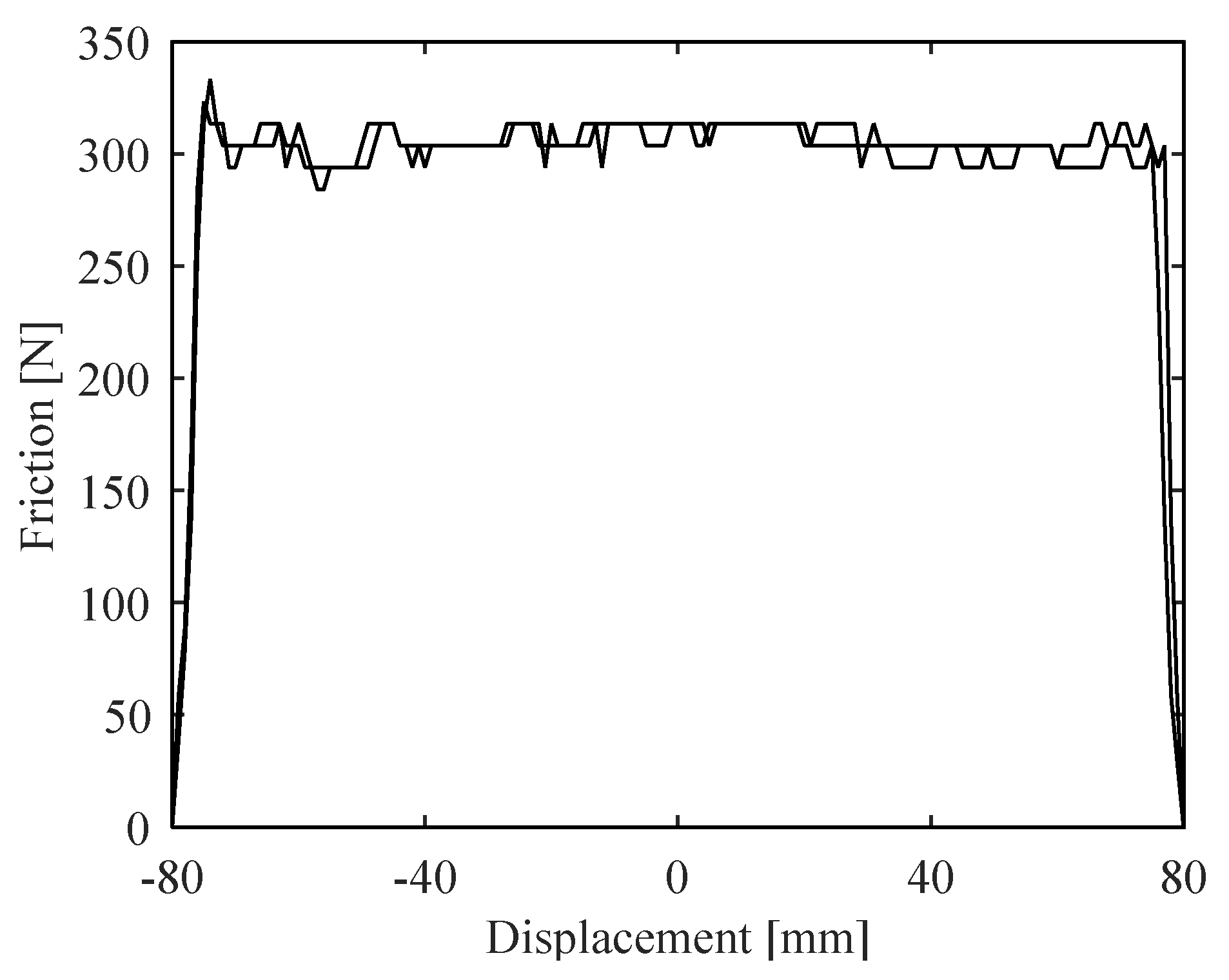
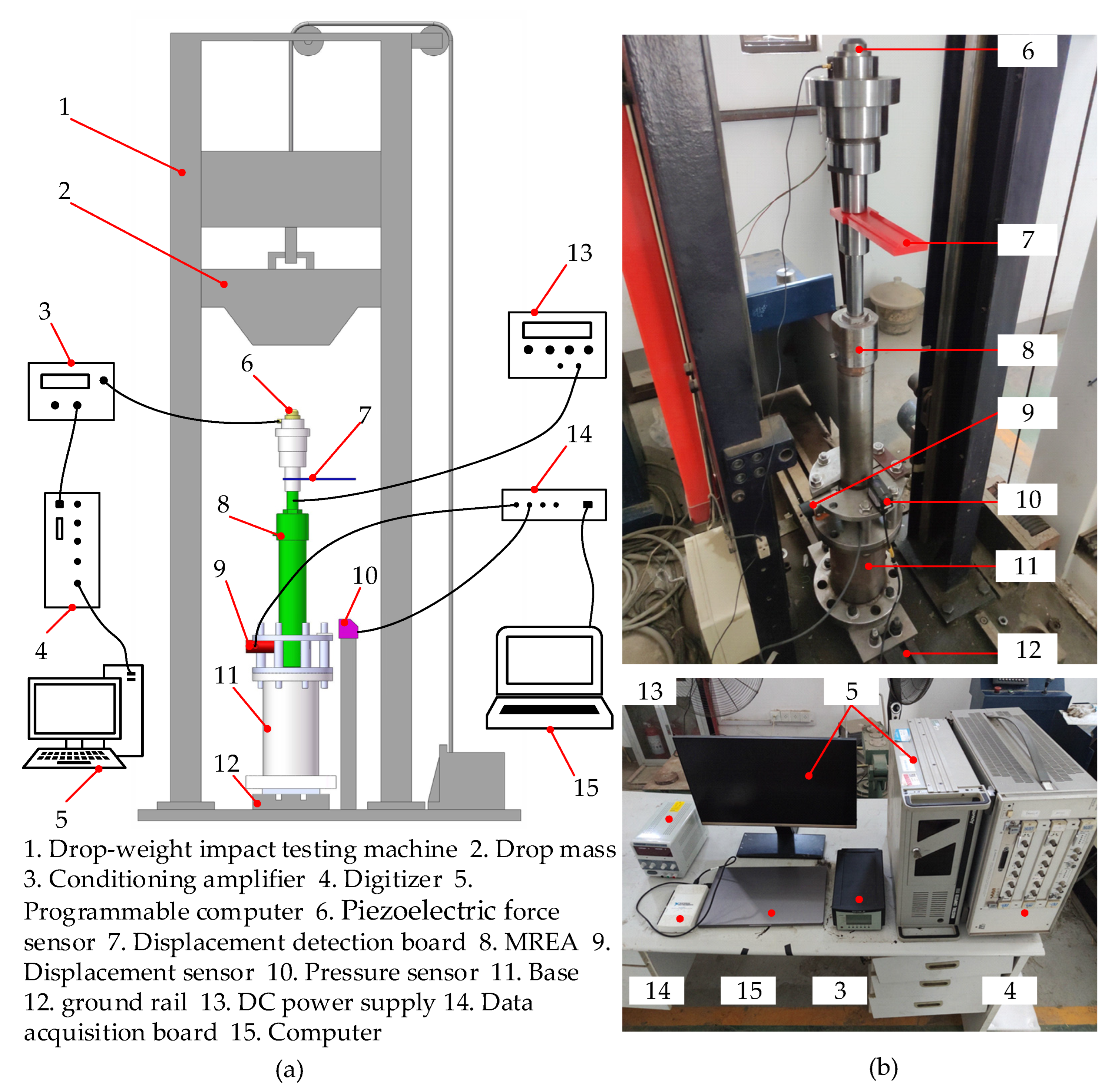
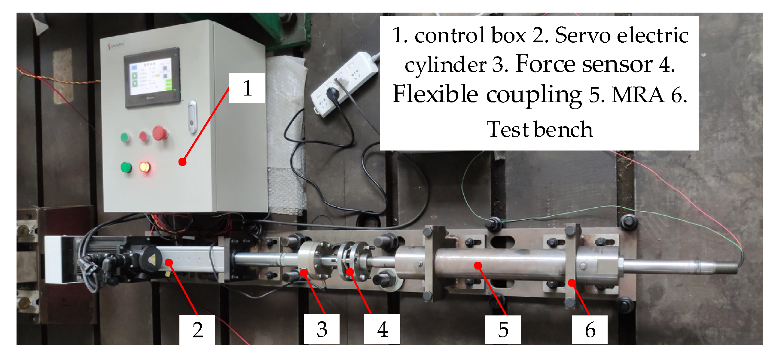
5. Experimental Setup

A drop-weight impact test system was set up to validate the unsteady numerical model, and the schematic and picture of the test system are shown in Figure 7. The experimental setup is mainly composed of the drop-weight impact testing machine (JL-1000), MRA, sensors, and data acquisition devices. The drop-weight impact testing machine was used to conduct the impact test. The lower end of the base was connected to the ground rail, and the upper end was fixed to the hydraulic cylinder. The drop-weight impact testing machine’s control system can control the lifting and release of the drop mass. Furthermore, the drop mass is 30 kg and moves along the track. During the impact process, the piston rod was subjected to the axial impact force, and the hydraulic cylinder remained stationary. Concurrently, the MR fluid was squeezed by the piston head and flowed from the extrusion chamber to another chamber through the narrow-long gap. The MRA was supplied with current via the DC power supply. Excitation currents of 0.5, 1, and 2 A were used in drop testing at a drop height of 0.7 m.

Table 1. Main parameters of the MRA.

Parameters	Value
Piston rod diameter, D0	30 mm
Piston head diameter, D1	54 mm
Inner diameter of hydraulic cylinder, D2	56 mm
Height of the gap, d	1 mm
Total length of the gap, L	120 mm
Total length of the activated region, La	60 mm
MR fluid density, ρ	2650 kg/m3

lists the main parameters of the MRA.

The dynamic data of the MRA during impact was tested using sensors and data acquisition devices. The displacement detection board was firmly connected to the piston rod in order to reflect the laser displacement sensor’s (IL-600, KEYENCE) test signal. The pressure sensor (PN3570, ifm) was screwed onto the hydraulic cylinder to test the pressure change in the extrusion chamber. The test signals of the pressure sensor and laser displacement sensor are transmitted to the computer through the data acquisition board for storage, and the sampling rate is 10 K. A piezoelectric force sensor (8231-C, B&K) was mounted at the top of the piston rod to assess the impact force of the drop mass on the piston rod. The conditioning amplifier amplified the piezoelectric force sensor test signal, which was then sent to the digitizer at a sampling rate of 200 K. The digitizer processed and presented the impact force test data on the screen of the programmable computer, allowing for real-time observation of the impact force change process. A rubber gasket was placed on the top end of the piezoelectric force sensor for all testing to protect the sensor from metal-to-metal impact and reduce test signal noise.

The time history curves of the impact force, pressure, and displacement obtained from the test re plotted in Figure 8. The impact force exhibits several pulses under different excitation currents as shown in Figure 8a. Furthermore, the initial impact pulse’s peak force is enormous, and then, the peak force of the impact pulse gradually drops. In the later stage of the impact process, the impact force changes gently and decreases gradually. The piston rod will cause significant instantaneous acceleration at the corresponding time of the initial peak of the impact force. The overall trend of impact force increases as excitation currents increase, but duration decreases. The change in pressure in the extrusion chamber under the impact force excitation displays a typical dynamic response as shown in Figure 8b. The initial pressure peak is high, but it fluctuates and then gradually drops. With increasing the excitation current, the field-dependent pressure in the activated region increases, so the overall trend of the pressure increases. The duration of the impact force and pressure is roughly the same for same excitation currents. In terms of momentum, raising the excitation current increases MRA’s hydraulic resistance, resulting in a shorter piston rod movement time for the same impact momentum. The displacement of the piston rod reduces as the excitation current is increased as seen in Figure 8c. From the perspective of energy, raising the excitation current increases the MRA’s hydraulic resistance, leading to a reduction in piston rod movement displacement for the same impact energy. The enormous instantaneous acceleration of the piston rod makes the displacement detection plate distort and shake during the impact process, causing the displacement test data to fluctuate over time.

As shown in Figure 9, a servo electric cylinder (BL70) was used to test the friction of the MRA when MR fluid was not injected into the inner chamber. The front end of the electric cylinder’s lead screw was fitted with a force sensor (DY-2T), which was then connected to the piston rod of the MRA via a flexible connection. The piston rod was driven at a constant speed of 5 mm/s by the servo electric cylinder. Concurrently, the force sensor was utilized to test the friction of the piston rod, and the test signal was collected and stored by the control box. Figure 10 shows the test data for the friction of the piston rod in the extension stroke for two consecutive cycles. The variability in friction is relatively tiny, approximately 300 N. Thus, the friction is taken as a fixed value of 300 N during impact to simplify the study.

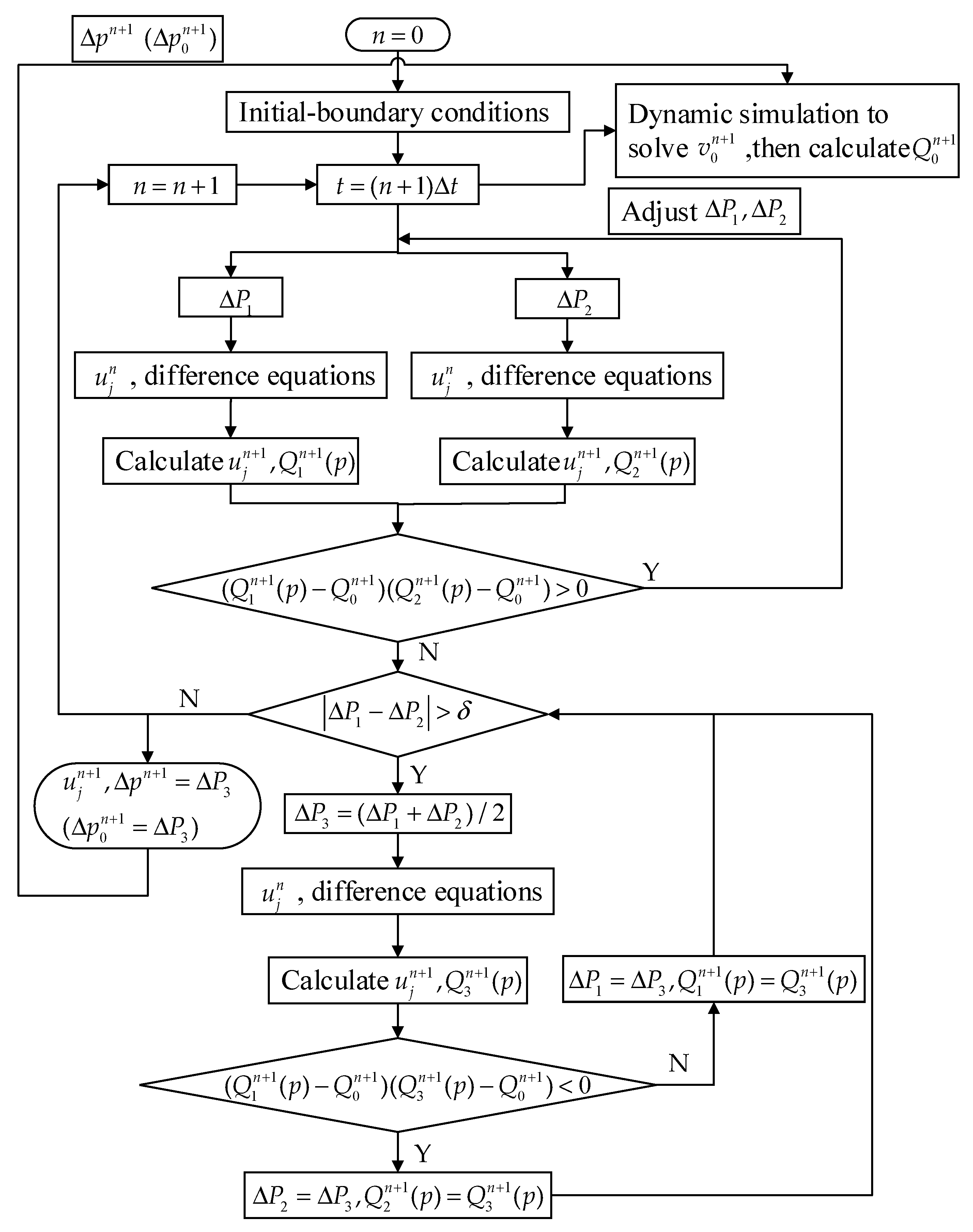
6. Numerical Simulation Calculation

The MRA’s hydraulic cylinder was fixed during impact, and the piston rod was subjected to the axial impact force. Accordingly, the piston rod’s motion is a rigid body motion with a single degree of freedom, and its dynamic equation is given as

$$m{a}^{n+1}=F_{\mathrm{i}}{}^{n+1}-F^n-F_{\mathrm{f}},$$

(24)

where

$$F^{n+1}=A_p\Delta P^{n+1}.$$

(25)

Here, $m$ is the mass of the piston head, piston rod, and its connecting parts; $a^{n+1}$ is the instantaneous acceleration of the piston rod at time $(n+1)\Delta t$; $F_i{}^{n+1}$ is the impact force obtained from the test data; $F^n$ is hydraulic resistance of the MRA at time $n\Delta t$, and $F^0=0$.

The velocity and displacement of the piston rod are deduced by numerical integration can be written as

$$v_0^n={\displaystyle \sum _{i=1}^n{a}^i\Delta t},$$

(26)

$$x^n={\displaystyle \sum _{i=1}^n{v}_0^i\Delta t},$$

(27)

where $x^n$ is the piston rod displacement at time $n\Delta t$.

The calculation program (refer to Supplementary Materials) was compiled in MATLAB to compute the unsteady flow field in the narrow-long gap and the kinematic parameters of the piston rod based on the unsteady numerical model and impact force. Figure 11 shows the flowchart for the unsteady numerical model, and following are the specific solution steps:

• At the initial time $n=0$, the unsteady governing PDE is established, and the initial-boundary conditions are determined.
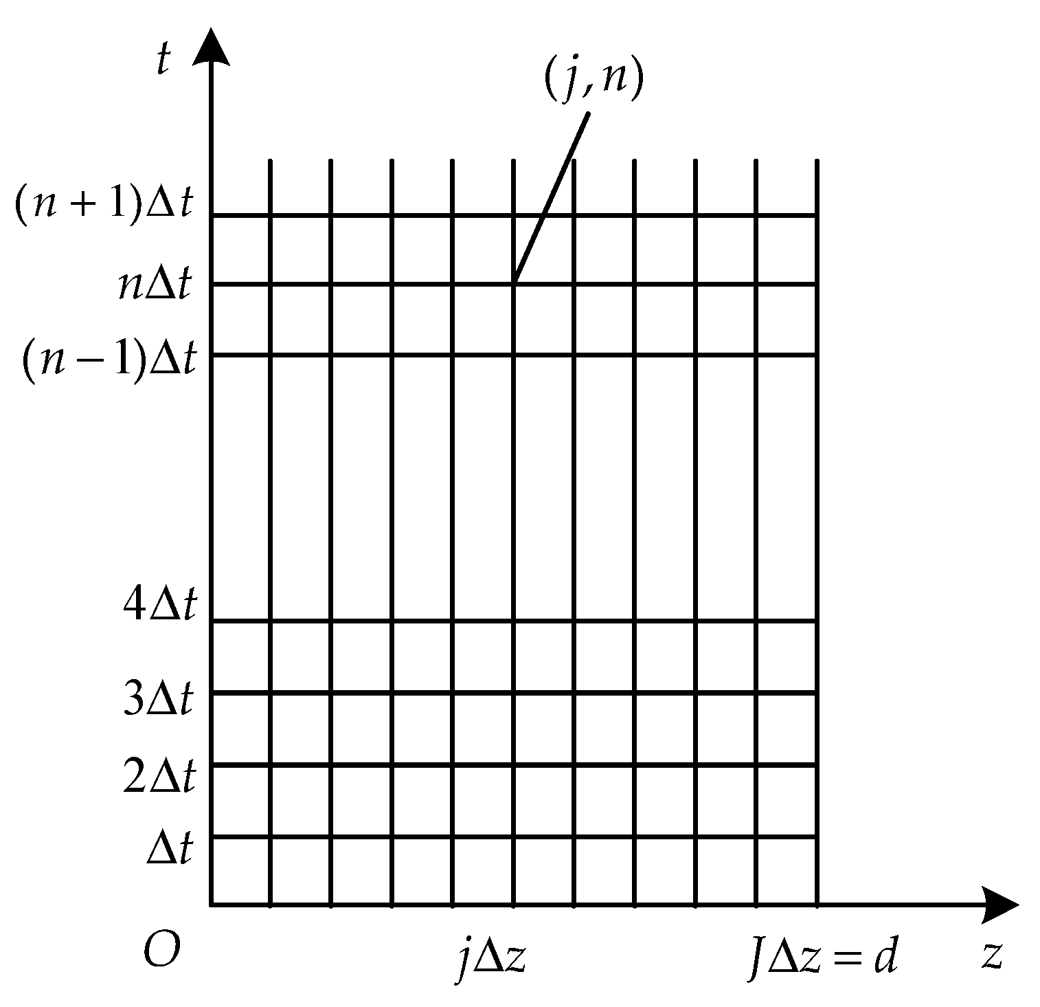
• The space-time 2D solution domain is discretized. The governing PDE is translated into implicit partial difference equations according to the finite difference method, and the initial-boundary conditions are transformed into the discrete scheme.
• The moving boundary velocity $v_0^{n+1}$ is calculated from Equations (23)–(26), and the volume flow rate $Q_0^{n+1}$ is calculated from Equations (18) and (19).
• The starting values of $\Delta P_1=-1\times {10}^{10}\mathrm{Pa}/\mathrm{m}$ and $\Delta P_2=1\times {10}^{10}\mathrm{Pa}/\mathrm{m}$ are used to define the interval $[\Delta P_1,\Delta P_2]$, which contains the numerical solution of the pressure gradient. Substitute $\Delta P_1,\Delta P_2$ into Equations (12)–(16) and consider Equations (20)–(22) for the whole activated region. Similarly, substitute $\Delta P_1,\Delta P_2$ into Equations (11) and (16) and consider Equations (20)–(22) for the whole inactivated region. The judgment condition $f(\Delta P_1)f(\Delta P_2)<0$ is used to determine if the pressure gradient solution $\Delta p^{n+1}$ (or $\Delta p^{n+1}$) is within the stated interval. If $\Delta p^{n+1}$ (or $\Delta p^{n+1}$) does not fall inside the interval, increase the interval range and judge again.
• Iterative calculation yields the numerical solution $\Delta p_0^{n+1}$ (or $\Delta p^{n+1}$) of pressure gradient based on the mass conservation, continuity equation, and bisection method. Substituting $\Delta P_1$ and the interval midpoint $\Delta P_3=(\Delta P_1+\Delta P_2)/2$ into Equations (12)–(16) and considering Equations (20)–(22) for the whole activated region deduces the corresponding volume flow rate in the gap $Q_1^{n+1}(p)$ and $Q_3^{n+1}(p)$, respectively. Similarly, substituting $\Delta P_1$ and the interval midpoint $\Delta P_3=(\Delta P_1+\Delta P_2)/2$ into Equations (11) and (16) and considering Equations (20)–(22) for the whole inactivated region deduces the corresponding volume flow rate in the gap $Q_1^{n+1}(p)$ and $Q_3^{n+1}(p)$, respectively. Tolerance $\delta =1\times {10}^{-5}\mathrm{Pa}/\mathrm{m}$ is defined. If $f(\Delta P_1)f(\Delta P_3)<0$, set $\Delta P_2=\Delta P_3,Q_2^{n+1}(p)=Q_3^{n+1}(p)$; if $f(\Delta P_1)f(\Delta P_3)\ge 0$, set $\Delta P_1=\Delta P_3,Q_1^{n+1}(p)=Q_3^{n+1}(p)$, then repeat the procedure. The iteration continues until the length of the interval is smaller than the tolerance, i.e., $\left|\Delta P_1-\Delta P_2\right|<\delta$, and the numerical solution of the pressure gradient $\Delta p^{n+1}$(or $\Delta p_0^{n+1}$) is found.
• Substitute the numerical solution of the pressure gradient $\Delta p^{n+1}$ into the Equations (12)–(15) to calculate the mesh points velocity $u_j^{n+1}$ for the whole activated region. Similarly, substitute the numerical solution of the pressure gradient $\Delta p_0^{n+1}$ into the Equation (11) to calculate the mesh points velocity $u_j^{n+1}$ for the total inactivated region.
• Output the kinematic parameters of the moving boundary (or piston rod) as well as the mesh points velocity and pressure gradient in the gap.
• $n=n+1$; repeat steps 3–7.

It is worth noting that if the velocity of the moving boundary (or piston rod) is known, it could be directly entered into the aforementioned unsteady numerical model to solve the unsteady flow field in the gap.

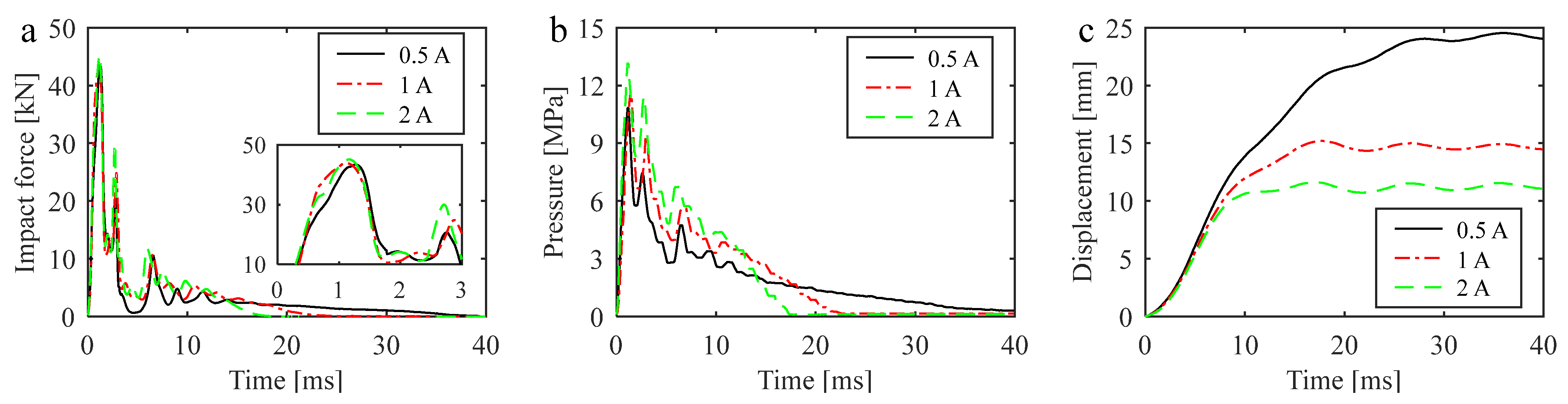
7. Results and Discussion

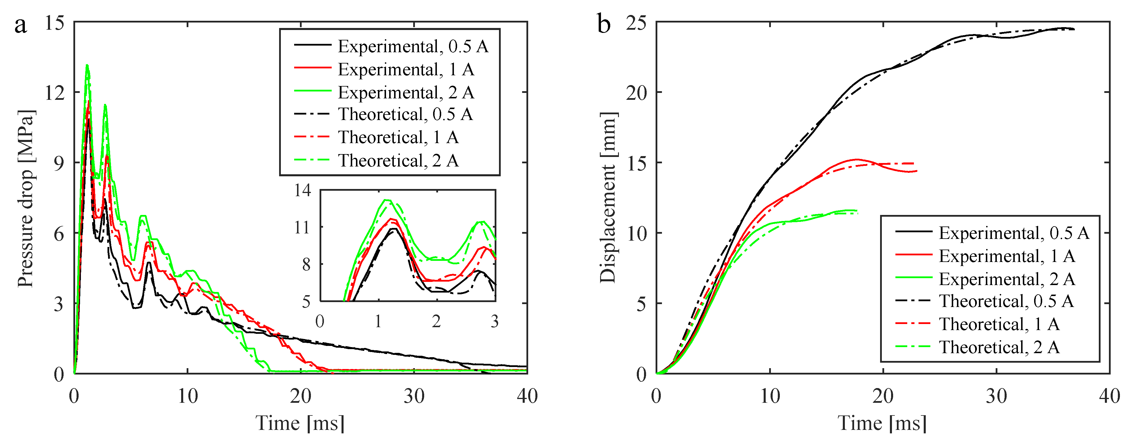
7.1. Model Results and Analysis

The experimental results are compared to the theoretical values of the pressure drop and displacement obtained from numerical simulation for different excitation currents under impact as illustrated in Figure 12. Figure 12a shows that the theoretical pressure drop value can accurately predict the peak value and change the tendency of the gap pressure drop, implying that the unsteady numerical model can help predict the dynamic change process of the unsteady flow field’s pressure drop in the gap. The theoretical value of displacement is in agreement with the experimental results as shown in Figure 12b, and the difference between them is primarily due to the fluctuation of the displacement test data. The accuracy of the unsteady numerical model is confirmed by the comparison of the theoretical value and experimental data of the pressure drop and displacement.

The kinematic parameters of the piston rod determine the volume flow rate as well as the dynamic changes in velocity profiles and pressure drop of the unsteady flow field in the gap. Figure 13 depicts the theoretical values of piston rod velocity and acceleration under impact for different excitation currents. The piston rod velocity increases rapidly at first, then gradually decreases after reaching the peak value, and decreases faster with increasing excitation currents as shown in Figure 13a. Due to the large peak value of piston rod velocity, there will be a wide range of volume flow rate in the gap. As seen in Figure 13b, the initial peak values of piston rod acceleration are huge and fluctuate noticeably, which is caused by the enormous initial peak value of the impact force and multiple peaks. Furthermore, the acceleration movement of the piston rod causes the MR fluid accelerate to flow in the gap, causing the gap pressure drop to be affected by the flow inertia. On the other hand, the hydraulic resistance of the MRA increases as the excitation currents increase, leading to the peak velocity and peak acceleration of the piston rod under impact force to decrease slightly.

The gap pressure drop in Figure 12a is analyzed in combination with the kinematic parameters of the piston rod in Figure 13. In the initial stage, both the volume flow rate and the flow inertia in the gap are large, causing the gap pressure drop to also be large. After that, the volume flow rate gradually decreases, resulting in a decrease in the gap pressure drop.

7.2. Velocity Profiles and Acceleration Profiles of the MR Fluid in the Gap

MR fluid is Newtonian fluid in the inactivated region. However, MR fluid is bi-viscous (non-Newtonian) fluid in the activated region. Furthermore, the viscosity in the pre-yield region is significantly greater than that in the post-yield region, and the parameters of the constitutive model can be adjusted by the excitation current. Thus, the dynamic changes of the MR fluid in the unsteady flow field’s velocity profiles and acceleration profiles in the activated region are more complex and interesting than those in the inactivated region. In the activated region, there are pre-yield and post-yield regions, and the boundary point is where the pre-yield and post-yield regions meet. Additionally, the fluid’s shear stress at the boundary point is transition stress. The shear stress of MR fluid in the pre-yield region is lower than the transition stress, whereas the shear stress of MR fluid in the post-yield region is higher. The mesh points velocity of each time step is calculated using the above unsteady numerical model for different excitation currents, and then, the mesh points acceleration is calculated using Equation (9).

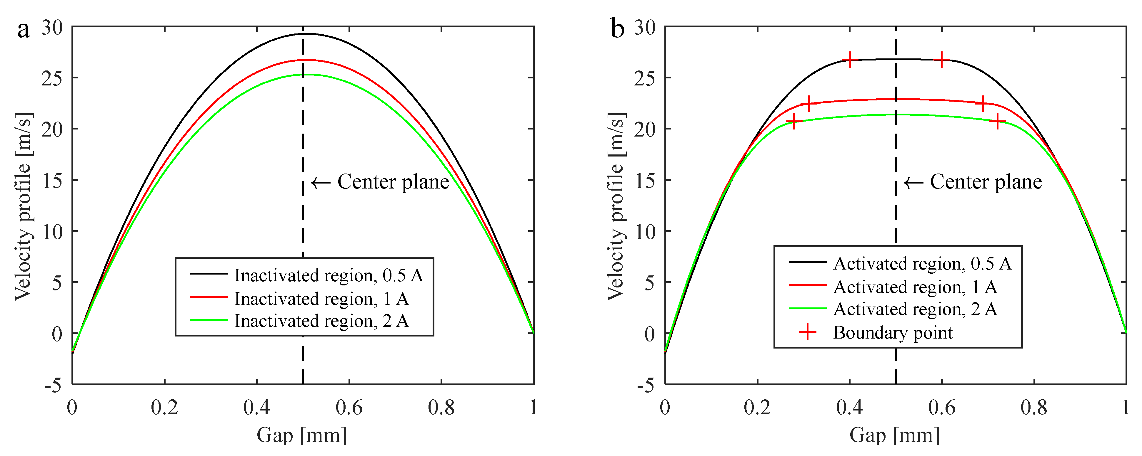
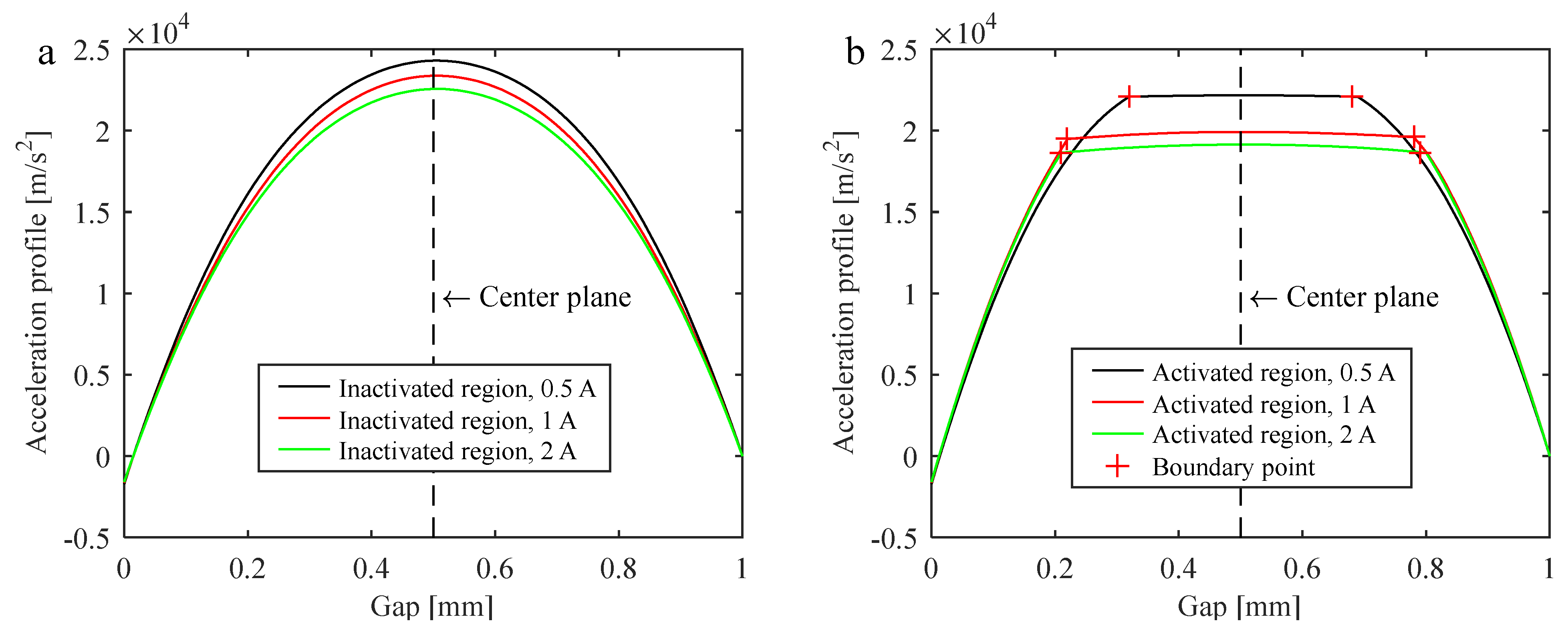
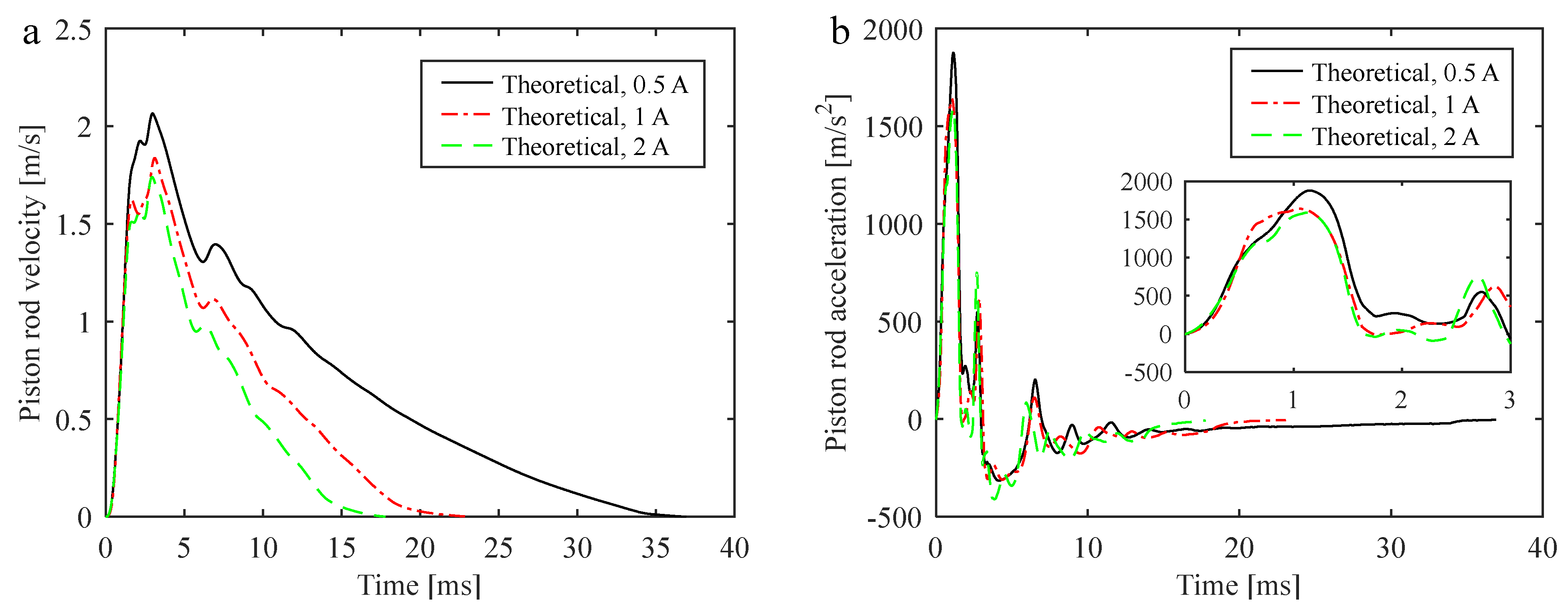
7.2.1. Peak Velocity Profiles and Peak Acceleration Profiles

Figure 14 depicts the inactivated and activated regions’ peak velocity profiles (at the peak time of piston rod velocity) for different excitation currents. Analyzing in conjunction with Figure 13a, the peak velocity of the piston rod decreases as the excitation current increases, resulting in the decrease of volume flow rate in the gap. As a result, the overall trend of the peak velocity profiles in the inactivated and activated regions is decreasing. In addition, the MR fluid velocity in the gap is high. For example, the MR fluid velocity in the center of the gap for the inactivated and activated regions is 29.28 m/s and 26.78 m/s, respectively, when the excitation current is 0.5 A. The volume flow rate in the inactivated and activated regions is equal when the excitation current is the same, but the distribution of velocity profiles are obviously different. The velocity profiles in the inactivated region are parabolic as shown in Figure 14a, which is the typical velocity distribution of the parabolic governing PDE describing unsteady Newtonian fluid flow. The velocity profiles in the activated region has the pre-yield and post-yield regions as shown in Figure 14b. The pre-yield region is the middle region of the boundary points, and the two sides are the post-yield region. The velocity profiles in the pre-yield region are flat parabolas. Because the viscosity in the pre-yield region is obviously higher than in the post-yield region, the slope of the velocity profiles in the pre-yield region is obviously less than in the post-yield region. Furthermore, increasing the excitation current increases the transition stress of MR fluid, resulting in an increase in the thickness of the pre-yield region.

Figure 15 shows the inactivated and activated regions’ peak acceleration profiles (at the peak time of piston rod acceleration) for different excitation currents. According to Figure 13b, the peak acceleration of the piston rod decreases with increasing the excitation current, so the peak acceleration profiles of the inactivated and activated regions decrease as a whole. The peak acceleration profiles of the inactivated and activated regions gradually increase from the two boundaries to the central plane of the gap, indicating that the acceleration of the MR fluid is non-uniform in distribution. Additionally, the MR fluid acceleration in the gap is rather high. For instance, when the excitation current is 0.5 A, the fluid acceleration in the center of gap in the inactivated and activated regions is up to 2.43 × 10⁴ m/s² and 2.22 × 10⁴ m/s², respectively. Furthermore, the distribution of fluid acceleration profiles are obviously different for the inactivated and activated regions. The fluid acceleration profiles in the inactivated region are parabolic as shown in Figure 15a. The pre-yield region is located in the middle of the activated region’s boundary points, while the post-yield region is located on both sides as shown in Figure 15b. The peak acceleration profiles in the pre-yield region are parabolas with a small slope, whereas the slope of the post-yield region is large.

Remarkably, the maxima of the velocity profiles and acceleration profiles are located in the center of the gap for both the activated and inactivated regions.

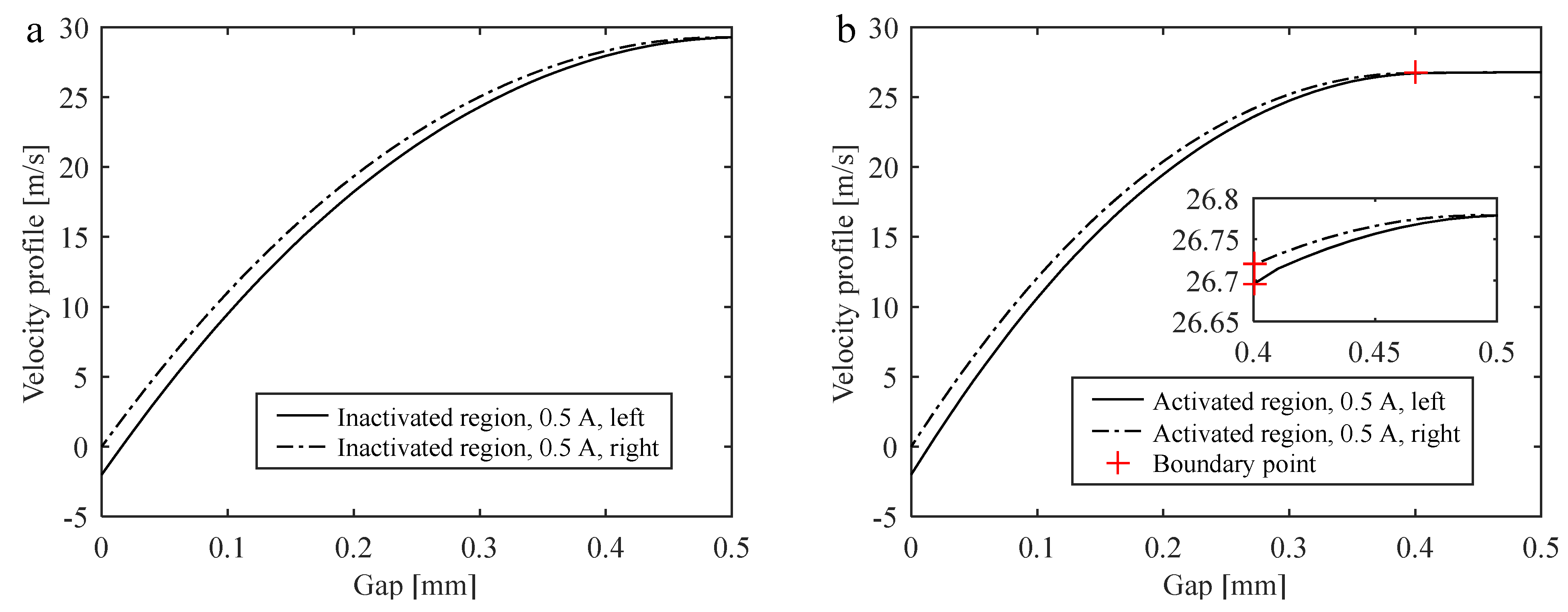
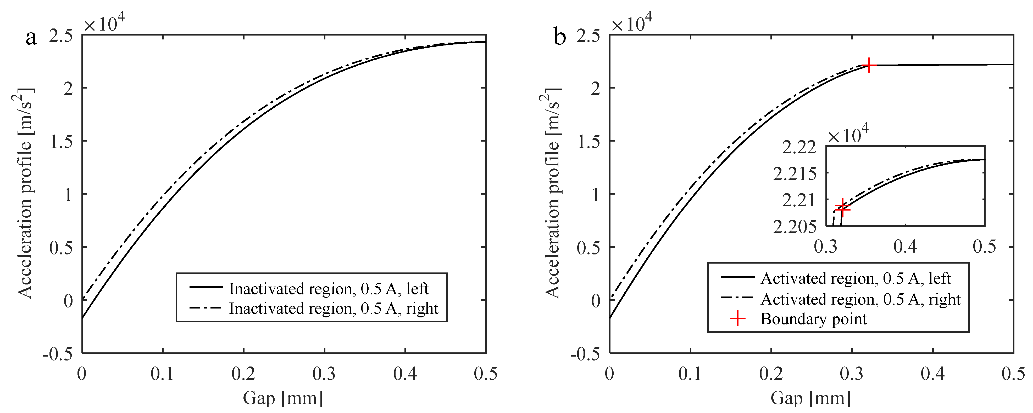
7.2.2. Asymmetric Distribution of the Flow Field

The unsteady flow field in the gap will be asymmetric to the center plane due to the movement of the moving boundary relative to the stationary boundary. Take, for example, the peak velocity and peak acceleration profiles for the excitation current is 0.5 A. As illustrated in Figure 16 and Figure 17, the peak velocity and peak acceleration profiles on the right side of the central plane (one side of the stationary boundary) are in mirror symmetry to the left side, and the influence of the moving boundary on the asymmetry of the unsteady flow field is investigated. For both the activated and inactivated regions, the velocity and acceleration profiles of the MR fluid on the left (one side of the moving boundary) are generally smaller than those on the right. Furthermore, from the boundary to the gap center, the difference value in the velocity (or acceleration) profiles of the MR fluid on the left and right sides gradually decreases. The difference value in the velocity (or acceleration) profiles of the MR fluid on the left and right sides in the pre-yield region is small for the activated region because the velocity (or acceleration) profiles distribution in the pre-yield region is flat. Interestingly, the thickness of the pre-yield region is symmetrical in relation to the center plane.

7.2.3. Space-Time Dynamic Distribution of the MR Fluid

Figure 18 shows the simulation-derived space-time dynamic distribution of the MR fluid velocity in the inactivated and activated regions for the 2 A excitation current. The velocity profiles along the gap in the inactivated region are parabolic as shown in Figure 14a. The velocity profiles of the activated region along the gap have the pre-yield and post-yield regions as shown in Figure 14b. The flat region in the middle of velocity profile is the pre-yield region with small slope, and the regions on both sides are the post-yield regions with large slope. This is mainly because the viscosity of MR fluid in the pre-yield region is greater than that in the post-yield region. The effect of volume flow rate on the velocity distribution in the gap is investigated in conjunction with Figure 13a. The fluid velocity changes dynamically with the gap coordinate and time variable as the volume flow rate changes. When the piston rod speed increases, the volume flow rate in the gap increases, and the overall trend of velocity profiles in the inactivated and activated regions increases. At the same time, the shear rate increases in the adjacent region of the pre-yield and post-yield regions lead to the increase of shear stress. MR fluid transits from the pre-yield region to the post-yield region when the transition stress is exceeded, and the thickness of the pre-yield region gradually decreases. In addition, as the volume flow rate changes, the change rate of fluid velocity with respect to time in the activated and inactivated regions gradually increases from the boundaries on both sides to the center plane along the time coordinate direction, indicating that the fluid acceleration is in non-uniform distribution throughout the gap.

In the process of increasing the piston rod velocity from 0.8 m/s to 1.2 m/s, the thickness of the pre-yield region in the activated region gradually decreases with the increase of volume flow rate as shown in Figure 19. The boundary point of the velocity profile is located at $z=0.19 \mathrm{mm}$ when $v_0$ is 0.8 m/s. The slope of the velocity profile at $z=0.19 \mathrm{mm}$ increases when $v_0$ increases to 1 m/s, resulting in the shear rate increases and the shear stress exceeding the transition stress. Consequently, the mesh point at $z=0.19 \mathrm{mm}$ transitions from the boundary point to the post-yield region. Similarly, the shear rate of the mesh point at $z=0.21 \mathrm{mm}$ on the velocity profile increases when $v_0$ increases from 1 m/s to 1.2 m/s, leading to the shear stress exceeding the transition stress, and the mesh point at $z=0.21 \mathrm{mm}$ transitions from the boundary point to the post-yield region. Therefore, as the volume flow rate in the activated region increases, the overall trend of the velocity profile increases, and the thickness of the pre-yield region decreases.

Figure 20 shows visually the thickness of the pre-yield region in the activated region changing over time in Figure 18b. In conjunction with Figure 13a, the thickness of the pre-yield region is closely related to the volume flow rate, and the thickness of the pre-yield region gradually decreases with the volume flow rate increases. Furthermore, the thickness of the pre-yield region is 1 mm when the volume flow rate is small, implying that all MR fluid in the activated region is located in the pre-yield region. Then, the thickness of the pre-yield region decreases to less than 1 mm as the volume flow rate increases, indicating that there is a transitional flow phenomenon in the activated region.

The magnetic flux density in the activated region changes as the excitation current changes, resulting in a difference in velocity profile due to the changing parameters of the MR fluid constitutive model. The velocity profiles of the activated region for different excitation currents under $v_0=0.5 \mathrm{m}/\mathrm{s}$ and $v_0=1 \mathrm{m}/\mathrm{s}$ are shown in Figure 21. When the volume flow rate in the gap is equal, the main difference in the velocity profiles is that the thickness of the pre-yield region grows as the excitation current increase. This is because increasing the excitation current increases the magnetic flux density of the activated region (see Figure 2), leading to an increase in the transition stress (refer to Figure 4).

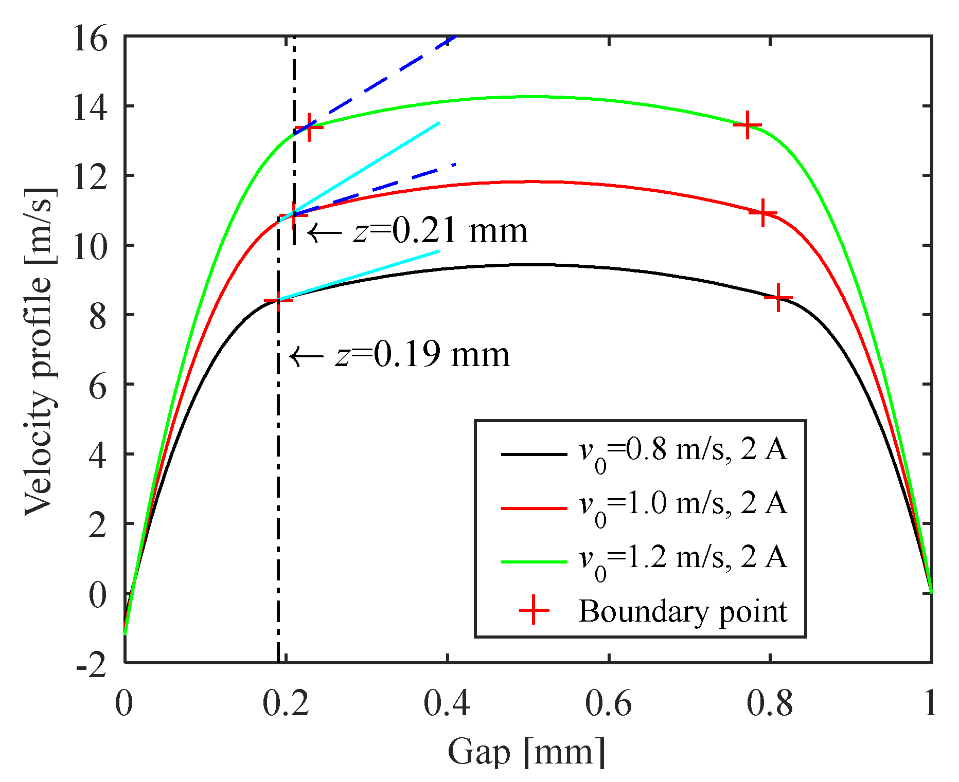
7.2.4. Transition Flow Phenomenon in the Activated Region

There is a transition flow phenomenon during the change of MR fluid volume flow rate in the activated region, according to the analysis results in Figure 20. Figure 22 depicts the space-time dynamic distribution of the MR fluid velocity and acceleration in the activated region during the transition flow stage for the 2 A excitation current. The shear stress of the MR fluid in the entire activated region is smaller than the transition stress when the volume flow rate is small. Meanwhile, the activated region contains only the pre-yield region, and the velocity and acceleration profiles are parabolic. Because the shear rate reaches its maximum on both sides at the boundary for the parabolic velocity profile, the shear stress at the boundary is the highest. With the increase in volume flow rate, the general trend of the velocity profiles increases, and so does the shear stress of the MR fluid at the boundary. When the shear stress exceeds the transition stress, MR fluid at the boundary first transits from the pre-yield to the post-yield region. Meantime, the activated region will have both a pre-yield and the post-yield region. Furthermore, more mesh points near the boundary transition to the post-yield region with the further increase of the volume flow rate, so the thickness of the pre-yield region gradually reduces.

There are apparent differences in velocity profiles and acceleration profiles before and after dynamic transition. Figure 23 shows visually the velocity profiles and acceleration profiles at time $t=0.35 \mathrm{ms}$ and $t=0.6 \mathrm{ms}$ in the activated region for the excitation current of 2 A. There is only the pre-yield region in the activated region before dynamic transition, and the velocity profiles and acceleration profiles are typical parabolas. After dynamic transition, the activated region has both the pre-yield and post-yield regions. Meanwhile, the velocity profiles and acceleration profiles of the pre-yield region are parabolic, and the slope is less than that of the post-yield region. In addition, the difference in acceleration profiles before and after the dynamic transition is more noticeable.

7.3. Influence of Mesh Density on Calculation Results of Unsteady State Model

The effect of mesh density on the convergence of the calculation results of the unsteady numerical model is investigated under the constraint of the numerical scheme stability. The space steps are 0.1, 0.05, 0.02, and 0.01 mm for the gap bisections J of 10, 20, 50, and 100, respectively. Equation (17) is used to calculate the corresponding time step $\Delta t$.

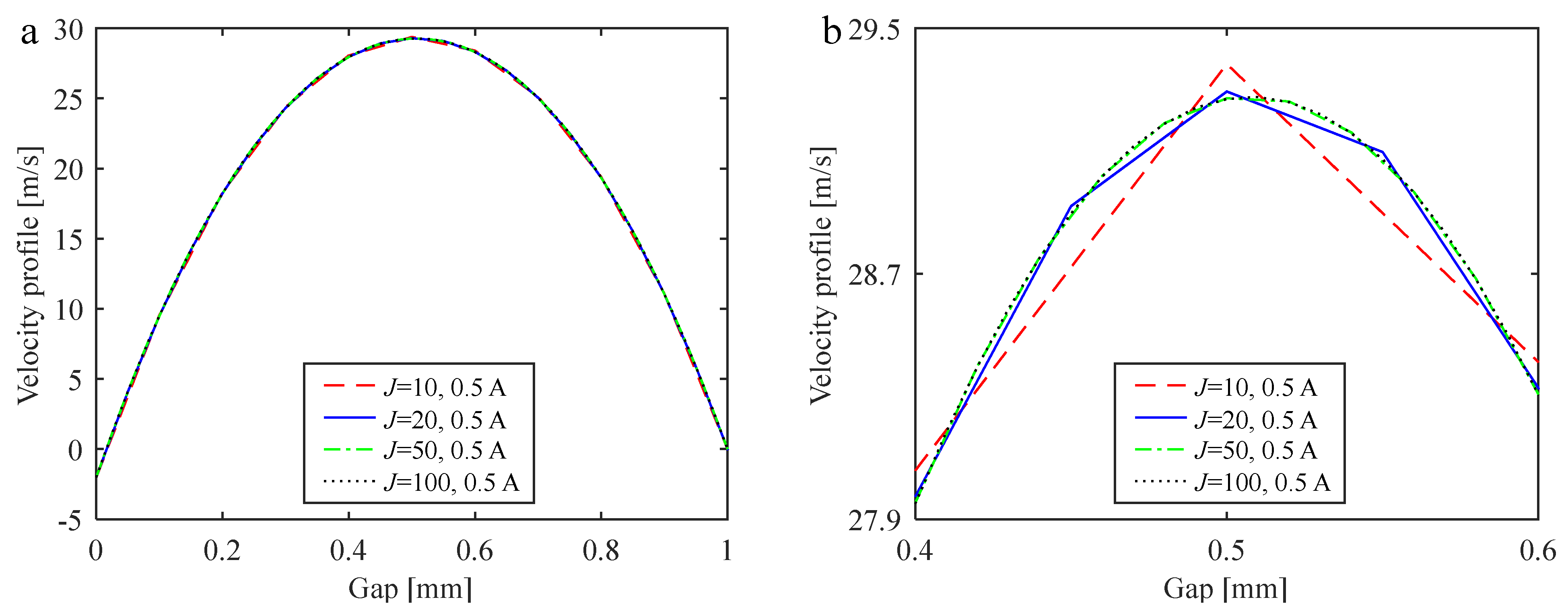
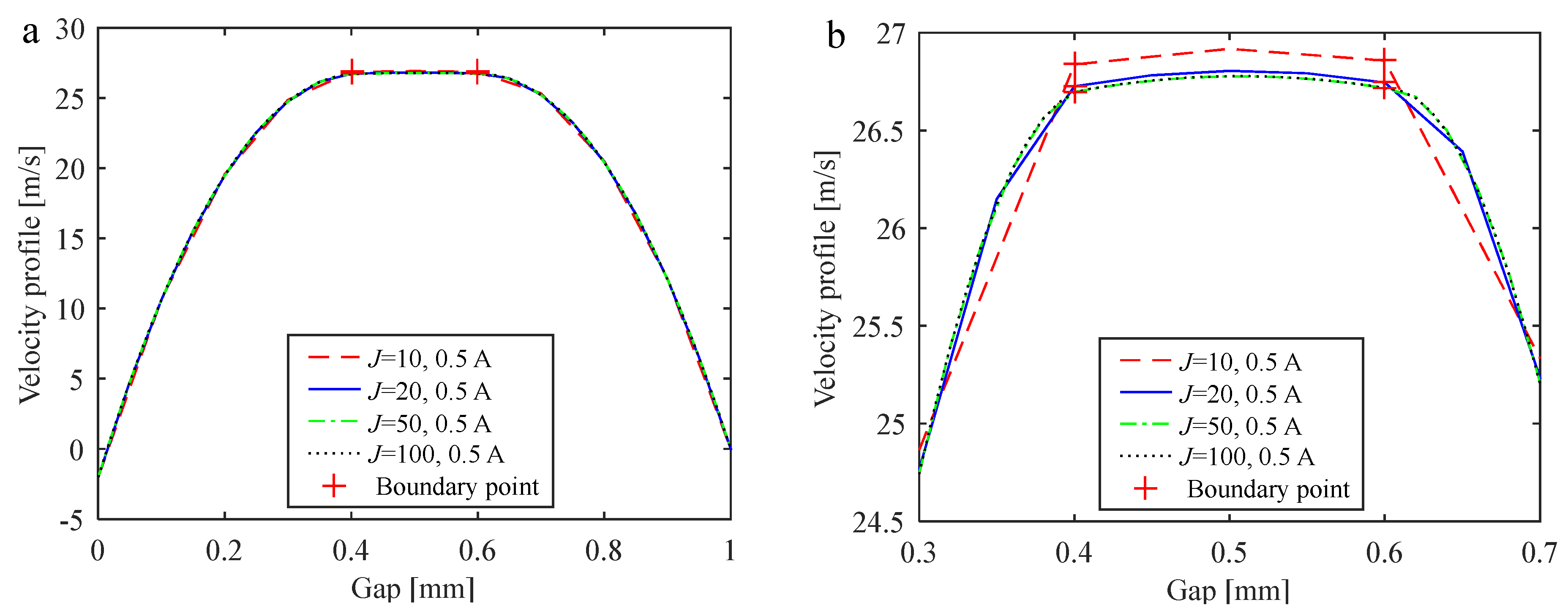
7.3.1. Influence of Mesh Density on the Velocity Profiles

Using the peak velocity profiles in the gap as an example with the 0.5A excitation current, the velocity profiles of the MR fluid simulation-derived under different mesh density are compared. The peak velocity profiles of the inactivated and activated regions for different mesh density, as well as their local expansion, are shown in Figure 24 and Figure 25. The general trend of the velocity profiles of the inactivated and activated regions is consistent under different mesh density, and the thickness of the pre-yield zone is equal for the activated region as shown in Figure 24a and Figure 25a. Additionally, the velocity profiles tend to be smoother as mesh density increases as seen in Figure 24b and Figure 25b, which can more precisely describe the smooth velocity profiles in the actual unsteady flow field.

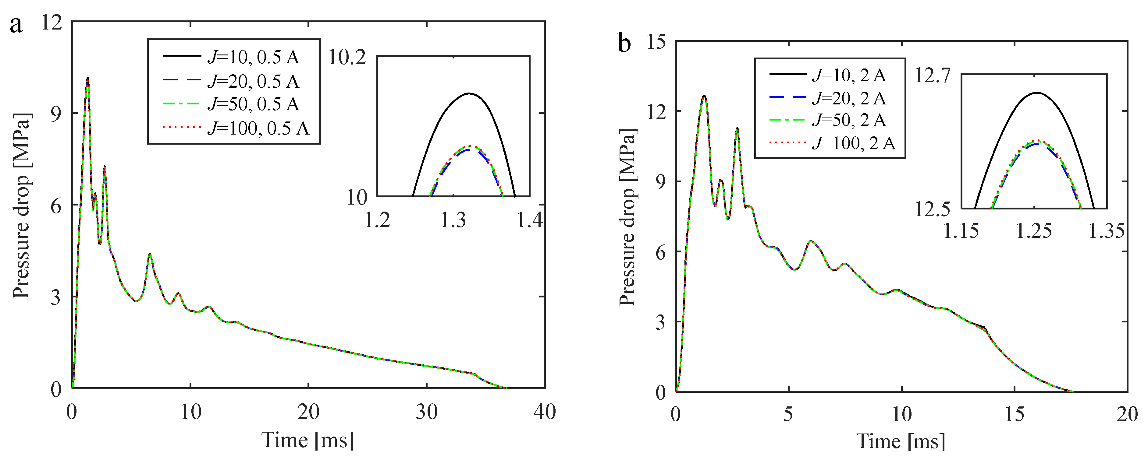
7.3.2. Influence of Mesh Density on the Pressure Drop

Figure 26 shows the pressure drop of the gap simulation-derived for different mesh density under the excitation currents of 0.5 and 2 A. The pressure drop shows an excellent agreement for different mesh density, indicating that the unstable numerical model has good stability. On the other hand, observing the local enlargement of the peak pressure drop in Figure 26, the peak pressure drop computed for different mesh density is slightly different, and the peak pressure drops progressively approach each other as the mesh density increases. The accuracy of the numerical approach of the finite difference method improves with increasing mesh density according to its properties. The numerical solution of peak pressure drop for $J=100$ is used as the analyses’ reference solution. The impact of mesh density on the convergence of numerical solutions is investigated using the relative difference values between the peak pressure drop with J of 10, 20, and 50 and the peak pressure drop with J of 100 as shown in

Table 2. Relative difference values of peak pressure drop for different mesh density (MPa).

	0.5 A	1 A	2 A
J = 10	7.479 × 10−2	7.960 × 10−2	7.099 × 10−2
J = 20	5.155 × 10−3	5.499 × 10−3	5.699 × 10−3
J = 50	5.611 × 10−4	1.993 × 10−4	1.592 × 10−3

. The table shows that the relative difference values in peak pressure drop for different mesh density are quite small and gradually decrease as mesh density increases, indicating that the proposed unsteady numerical model has good convergence.

8. Conclusions

This paper investigates the unsteady flow field generated by high-speed unsteady laminar boundary layer flow of the MR fluid as Newtonian fluid and bi-viscous fluid in the narrow-long gap with a magnetic-field-activated region and moving boundary, which is described by unsteady governing PDE and initial-boundary conditions. By establishing a new unsteady numerical model based on finite difference method, the unsteady governing PDE is solved, and the dynamic changes of the velocity profiles and pressure drop in the unsteady flow field are obtained. The accuracy of the unsteady numerical model is verified based on the experiment. The main conclusions are as follows:

• The acceleration profiles are in a non-uniform distribution along the gap’s height when MR fluid unsteady flow is in the gap. The pressure drop of the unsteady flow field in the gap is generated by the dynamic coupling of fluid viscosity and non-uniform flow inertia.
• The asymmetry of the unsteady flow field in the gap is caused by the moving boundary, and the maxima of the velocity and acceleration profiles occur in the center plane. The velocity and acceleration profiles on one side of the moving boundary are less than those on the other side of the fixed boundary with relation to the gap’s central plane, and the thickness of the pre-yield region is symmetrical about the center plane.
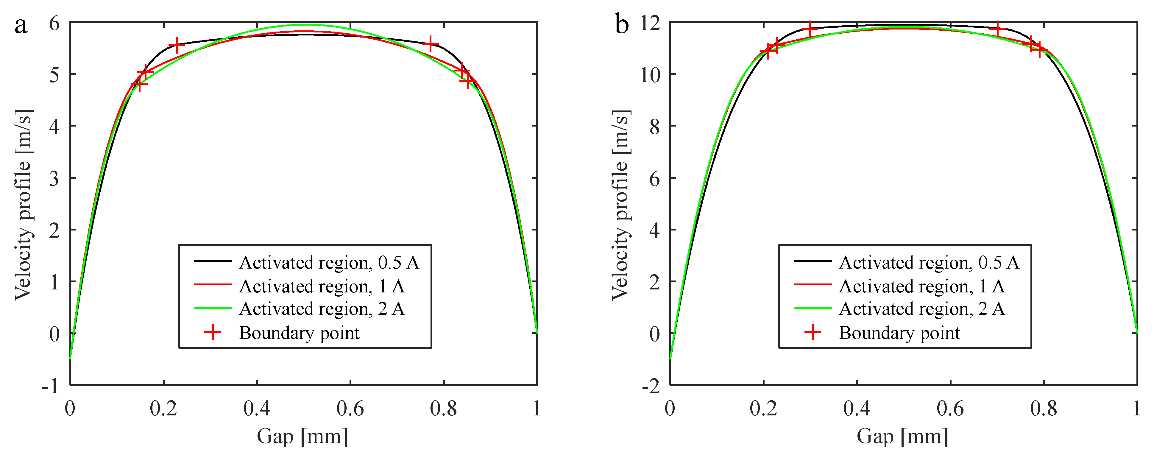
• When the excitation current is determined, the thickness of the pre-yield region in the activated region gradually decreases as the volume flow rate is increased. When the volume flow rate is determined, increasing the excitation current increases the transition stress of the MR fluid in the activated region, which increases the thickness of the pre-yield region.
• There is a transition flow phenomenon during the change of the MR fluid volume flow rate in the activated region. When the volume flow rate is small, the activated region only has the pre-yield region. However, as the volume flow rate increases, the post-yield region will appear on both sides of the boundary. Meanwhile, the distribution of velocity and acceleration profiles changes noticeably before and after the transition.
• When the mesh number J along the gap’s height is 10–100, the pressure drop of the gap solved by the unsteady numerical model has good convergence under the constraint of the numerical scheme stability.
• The proposed unsteady numerical model helps to better understand the properties of the unsteady laminar boundary layer flow of MR fluid in the gap, which may also be used as a theoretical reference for solving Newtonian and bi-viscous fluid unsteady laminar boundary layer flow problems.

References

1. Alam, M.K.; Bibi, K.; Khan, A.; Noeiaghdam, S. Dufour and Soret Effect on Viscous Fluid Flow between Squeezing Plates under the Influence of Variable Magnetic Field. Mathematics 2021, 9, 2404. [Google Scholar] [CrossRef]
2. Abderrahmane, A.; Qasem, N.A.A.; Younis, O.; Marzouki, R.; Mourad, A.; Shah, N.A.; Chung, J.D. MHD Hybrid Nanofluid Mixed Convection Heat Transfer and Entropy Generation in a 3-D Triangular Porous Cavity with Zigzag Wall and Rotating Cylinder. Mathematics 2022, 10, 769. [Google Scholar] [CrossRef]
3. Murillo-García, O.F.; Jurado, F. Adaptive Boundary Control for a Certain Class of Reaction–Advection–Diffusion System. Mathematics 2021, 9, 2224. [Google Scholar] [CrossRef]
4. Wilson, S. Squeezing flow of a Bingham material. J. Non-Newton Fluid Mech. 1993, 47, 211–219. [Google Scholar] [CrossRef]
5. Lin, C.J.; Yau, H.T.; Lee, C.Y.; Tung, K.H. System Identification and Semiactive Control of a Squeeze-Mode Magnetorheological Damper. IEEE ASME Trans. Mechatron. 2013, 18, 1691–1701. [Google Scholar] [CrossRef]
6. Kim, P.; Seok, J. Viscoplastic flow in slightly varying channels with wall slip pertaining to a magnetorheological (MR) polishing process. J. Non-Newton Fluid Mech. 2011, 166, 972–992. [Google Scholar] [CrossRef]
7. Jiang, R.L.; Rui, X.T.; Yang, F.F.; Zhu, W.; Zhu, H.T.; Jiang, M. Simulation and experiment of the magnetorheological seat suspension with a seated occupant in both shock and vibration occasions. Smart Mater. Struct. 2020, 29, 105008. [Google Scholar] [CrossRef]
8. Liu, X.H.; Wang, N.N.; Wang, K.; Chen, S.M.; Sun, S.S.; Li, Z.X.; Li, W.H. A new AI-surrogate model for dynamics analysis of a magnetorheological damper in the semi-active seat suspension. Smart Mater. Struct. 2020, 29, 037001. [Google Scholar] [CrossRef]
9. Saleh, M.; Sedaghati, R.; Bhat, R. Dynamic analysis of an SDOF helicopter model featuring skid landing gear and an MR damper by considering the rotor lift factor and a Bingham number. Smart Mater. Struct. 2018, 27, 065013. [Google Scholar] [CrossRef]
10. Yoon, J.Y.; Kang, B.H.; Kin, J.H.; Choi, S.B. New control logic based on mechanical energy conservation for aircraft landing gear system with magnetorheological dampers. Smart Mater. Struct. 2020, 29, 084003. [Google Scholar] [CrossRef]
11. Liu, S.C.; Chen, Z.Q.; Wang, X.Y.; Ko, J.M.; Ni, Y.Q.; Spencer, B.F., Jr.; Yang, G. MR damping system on Dongting Lake cable-stayed bridge. In Proceedings of the Smart Structures and Materials 2003: Smart Systems and Nondestructive Evaluation for Civil Infrastructures, San Diego, CA, USA, 18 August 2003; pp. 229–235. [Google Scholar] [CrossRef]
12. Kim, Y.; Langari, R.; Hurlebaus, S. Semiactive nonlinear control of a building with a magnetorheological damper system. Mech. Syst. Signal. Process. 2009, 23, 300–315. [Google Scholar] [CrossRef]
13. Yang, G.; Spencer, B.F., Jr.; Carlson, J.D.; Sain, M.K. Large-scale MR fluid dampers: Modeling and dynamic performance considerations. Eng. Struct. 2002, 24, 309–323. [Google Scholar] [CrossRef]
14. Ai, H.X.; Wang, D.H.; Liao, W.H. Design and modeling of a magnetorheological valve with both annular and radial flow paths. J. Intell. Mater. Syst. Struct. 2006, 17, 327–334. [Google Scholar] [CrossRef]
15. Hong, S.R.; John, S.; Wereley, N.M.; Choi, Y.T.; Choi, S.B. A Unifying Perspective on the Quasi-steady Analysis of Magnetorheological Dampers. J. Intell. Mater. Syst. Struct. 2007, 19, 959–976. [Google Scholar] [CrossRef]
16. Zhang, X.J.; Wu, R.C.; Guo, K.H.; Zu, P.Y.; Ahmadian, M. Dynamic characteristics of magnetorheological fluid squeeze flow considering wall slip and inertia. J. Intell. Mater. Syst. Struct. 2020, 31, 229–242. [Google Scholar] [CrossRef]
17. Chen, P.; Bai, X.X.; Qian, L.J. Magnetorheological fluid behavior in high-frequency oscillatory squeeze mode: Experimental tests and modelling. J. Appl. Phys. 2016, 119, 105101. [Google Scholar] [CrossRef]
18. Nguyen, Q.H.; Choi, S.B. Dynamic modeling of an electrorheological damper considering the unsteady behavior of electrorheological fluid flow. Smart Mater. Struct. 2009, 18, 055016. [Google Scholar] [CrossRef]
19. Zolfagharian, M.M.; Kayhani, M.H.; Norouzi, M.; Norouzi, M.; Jalali, A. Parametric investigation of twin tube magnetorheological dampers using a new unsteady theoretical analysis. J. Intell. Mater. Syst. Struct. 2019, 30, 878–895. [Google Scholar] [CrossRef]
20. Wang, J.; Li, Y.C. Dynamic Simulation and Test Verification of MR Shock Absorber under Impact Load. J. Intell. Mater. Syst. Struct. 2006, 17, 309–314. [Google Scholar] [CrossRef]
21. Zhang, X.W.; Yu, T.X.; Wen, W.J. Electro-rheological Cylinders used as Impact Energy Absorbers. J. Intell. Mater. Syst. Struct. 2010, 21, 729–745. [Google Scholar] [CrossRef]
22. Mao, M. Adaptive Magnetorheological Sliding Seat System for Ground Vehicles. Ph.D. Thesis, University of Maryland, College Park, MD, USA, 2011. [Google Scholar]
23. Mao, M.; Hu, W.; Choi, Y.T.; Wereley, N.M.; Browne, A.L.; Ulicny, J.; Johnson, N. Nonlinear modeling of magnetorheological energy absorbers under impact conditions. Smart Mater. Struct. 2013, 22, 115015. [Google Scholar] [CrossRef]
24. Haberman, R. Applied Partial Differential Equations with Fourier Series and Boundary Value Problems, 5th ed.; Pearson Education: Upper Saddle River, NJ, USA, 2012. [Google Scholar]
25. Woodford, C.; Phillips, C. Numerical Methods with Worked Examples: Matlab Edition, 2nd ed.; Springer: New York, NY, USA, 2012. [Google Scholar]
Figure 1. 2D structure schematic of the MRA.
Mathematics 10 02493 g001
Figure 2. Magnetic flux density along the annular gap for different excitation currents.
Mathematics 10 02493 g002
Figure 3. Bi-viscous rheological model.
Mathematics 10 02493 g003
Figure 4. Rheological behavior of MR fluid.
Mathematics 10 02493 g004
Figure 5. The flow problem: (a) parallel plates gap model; (b) typical velocity profiles of MR fluid in the activated and inactivated regions.
Mathematics 10 02493 g005
Figure 6. Solution domain of space-time discretization.
Mathematics 10 02493 g006
Figure 7. Drop-weight impact test system: (a) schematic and (b) picture.
Mathematics 10 02493 g007
Figure 8. Time history of the impact force, pressure, and displacement for different excitation currents under the drop height of 0.7 m.
Mathematics 10 02493 g008
Figure 9. Servo electric cylinder test bench.
Mathematics 10 02493 g009
Figure 10. Friction of the MRA.
Mathematics 10 02493 g010
Figure 11. Unsteady numerical model flowchart.
Mathematics 10 02493 g011
Figure 12. Comparison of the theoretical pressure drop and displacement values with experimental results for different excitation currents.
Mathematics 10 02493 g012
Figure 13. Theoretical values of piston rod velocity and acceleration for different excitation currents.
Mathematics 10 02493 g013
Figure 14. Peak velocity profiles for different excitation currents.
Mathematics 10 02493 g014
Figure 15. Peak acceleration profiles for different excitation currents.
Mathematics 10 02493 g015
Figure 16. Asymmetry of the velocity profiles for the excitation current of 0.5 A.
Mathematics 10 02493 g016
Figure 17. Asymmetry of the acceleration profiles for the excitation current of 0.5 A.
Mathematics 10 02493 g017
Figure 18. Space-time dynamic distribution of the MR fluid velocity in the inactivated and activated regions for the 2 A excitation current.
Mathematics 10 02493 g018
Figure 19. Velocity profiles with respect to various volume flow rate in the activated region.
Mathematics 10 02493 g019
Figure 20. Dynamic variation of the pre-yield region thickness for the 2 A excitation current.
Mathematics 10 02493 g020
Figure 21. Velocity profiles of the activated region for different excitation currents under v 0 = 0.5   m / s and v 0 = 1   m / s .
Mathematics 10 02493 g021
Figure 22. Space-time dynamic distribution of MR fluid velocity and acceleration during the transition flow stage in the activated region for the 2 A excitation current.
Mathematics 10 02493 g022
Figure 23. Velocity profiles and acceleration profiles at time t = 0.35   ms and t = 0.6   ms in the activated region for the excitation current of 2 A.
Mathematics 10 02493 g023
Figure 24. Peak velocity profiles of the inactivated region and its local enlargement for different mesh density under the excitation current of 0.5 A.
Mathematics 10 02493 g024
Figure 25. Peak velocity profiles of the activated region and its local enlargement for different mesh density under the excitation current of 0.5 A.
Mathematics 10 02493 g025
Figure 26. Pressure drop of the gap for different mesh density under the excitation currents of 0.5 and 2 A.
Mathematics 10 02493 g026