The basic concept of the neutron diffusion equation comes from applying Fick’s law to simplify the transport neutron equation; this simplification is fair where the behavior of the neutrons in the reactor is still reasonable. The simple neutron diffusion equation is used to express the neutrons moving in one velocity, and this is known as one-group case; for more reality, the neutrons will be divided in many velocities; this is known as the multi-group case. This study presents two multi-group subsystems where the reflector neutron diffusion equations subsystem is added to improve the work. This system consists of the fuel surrounded by a reflector, which saves the core and improves the fission inside it [
22,
23,
24,
25]. The mathematical manipulation for this system is studied next.
2.1. The Reactor Core Part
Here, the multi-group neutrons diffusion equations subsystem in the reactor core will be studied. Buckling in the core part is not unique, such as occurs in the bare reactor, there are two buckling named principal and alternate buckling, and each neutron flux is a linear combination of both principal and alternate buckling fluxes.
In HPM, fluxes depend on intersecting between constants connecting the fluxes, while the classical method depends on the buckling calculation.
Buckling is one of the most essential concepts in the nuclear reactor theory, as it represents the leaks of the neutrons in the reactor, which means it has an essential role in the stability of the nuclear reactor [
24].
The multi-group neutron diffusion equations for principal buckling in the reactor core are:
where
is the
group diffusion coefficient, and
is a constant that connects between fluxes in different energy groups of neutrons [
1], which is defined as follows:
Constants in Equation (2) have been defined in terms of different macroscopic cross-sections; the number of neutrons produced per fission for each group , and the fraction of fission neutrons emitted with energies in the th group is .
The time-independent diffusion system of the multi-group at the core of the spherical reactor, after substituting the Laplacian in the radial part dependent on spherical coordinates, can be written as:
This system of equations describes the behavior of the neutrons in the nuclear reactor where each flux
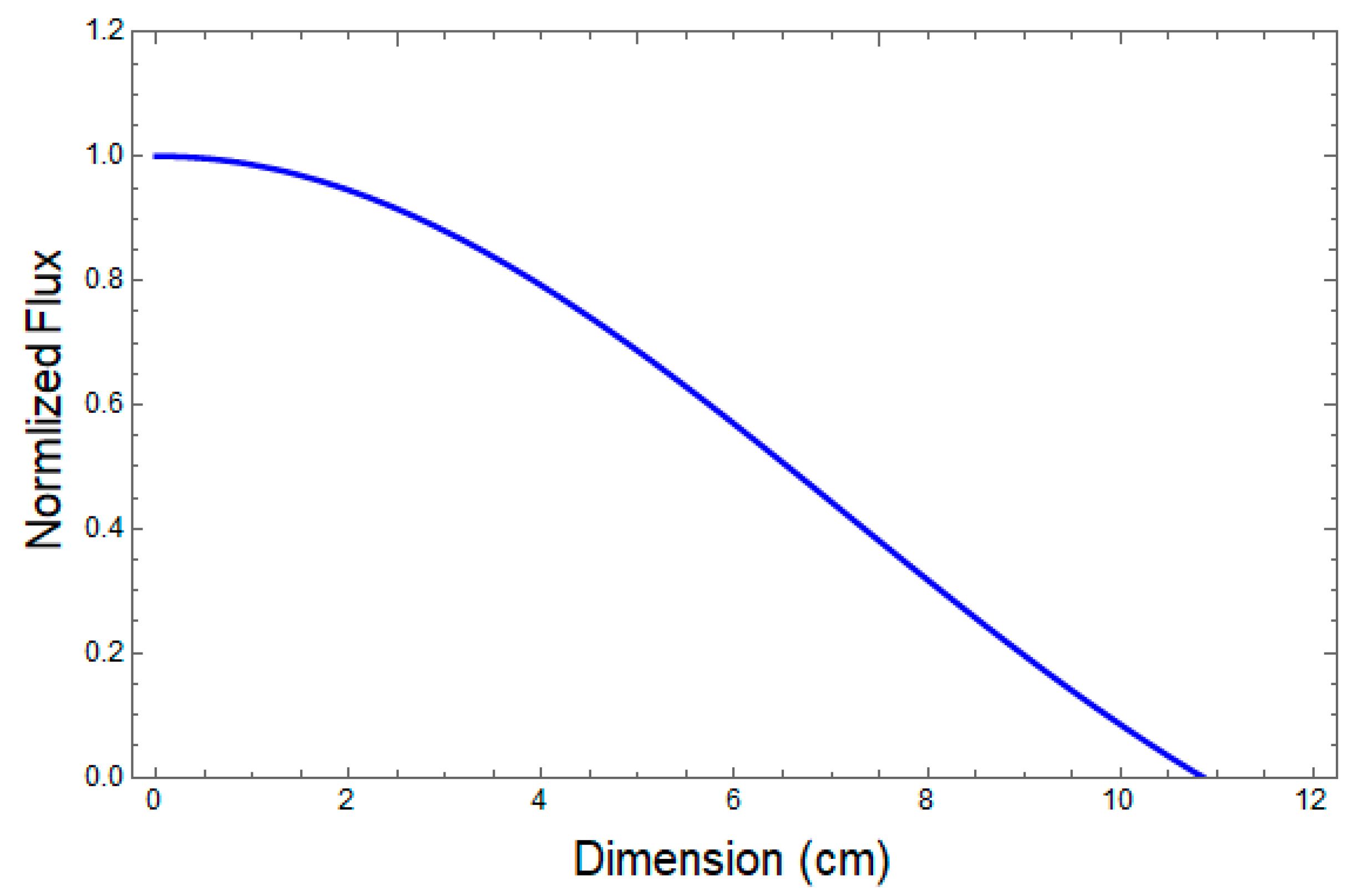
expresses the neutron flux with a specific energy. Each flux has a maximum value at the center of the reactor, while its derivative vanishes there, so the initial conditions can be written in the mathematical form as:
In order to solve these equations using HPM, we construct the homotopy [
6,
16] as:
where
is the homotopy,
is the original problem, and
is the simple problem.
Thus,
while the identical powers of
are:
The solution of the first component of Equation (7) is:
In summary, the fluxes, in this case, are given by:
Now, multi-group neutron diffusion equations for alternate buckling in the reactor core part will be:
where
is a constant connects between fluxes in different energy groups of neutrons. Respectively,
,
, and
are defined as:
Now, the diffusion system of multi energy groups of neutrons at spherical reactor can be written as:
One more time, the mathematical form of initial conditions can be written as:
In order to solve these equations using HPM, we construct the homotopy as:
To obtain a solution for this subsystem using HPM, the homotopy will be:
Taking identical powers of
as:
The solution of first component of Equation (18) is given by:
The other components are:
In summary, the fluxes of this part are:
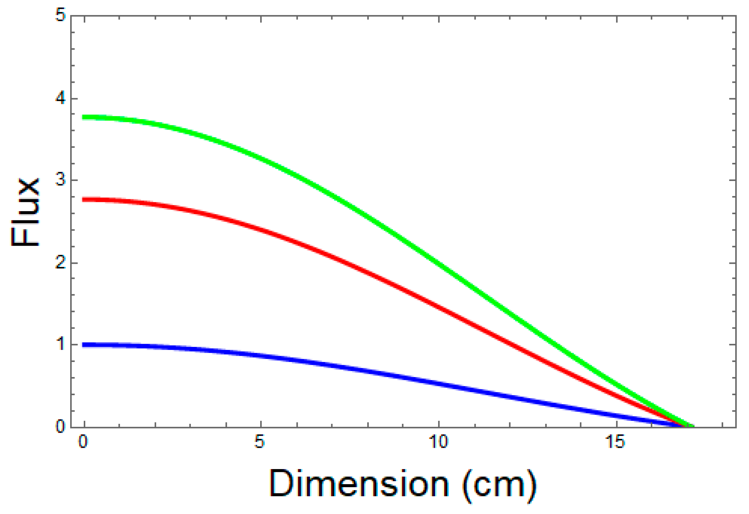
As is mentioned, the total flux of any group in the core part is linear combination of the two cases as:
Clearly, all fluxes should satisfy the needed boundary conditions.
2.3. The Core-Reflector Boundary Conditions
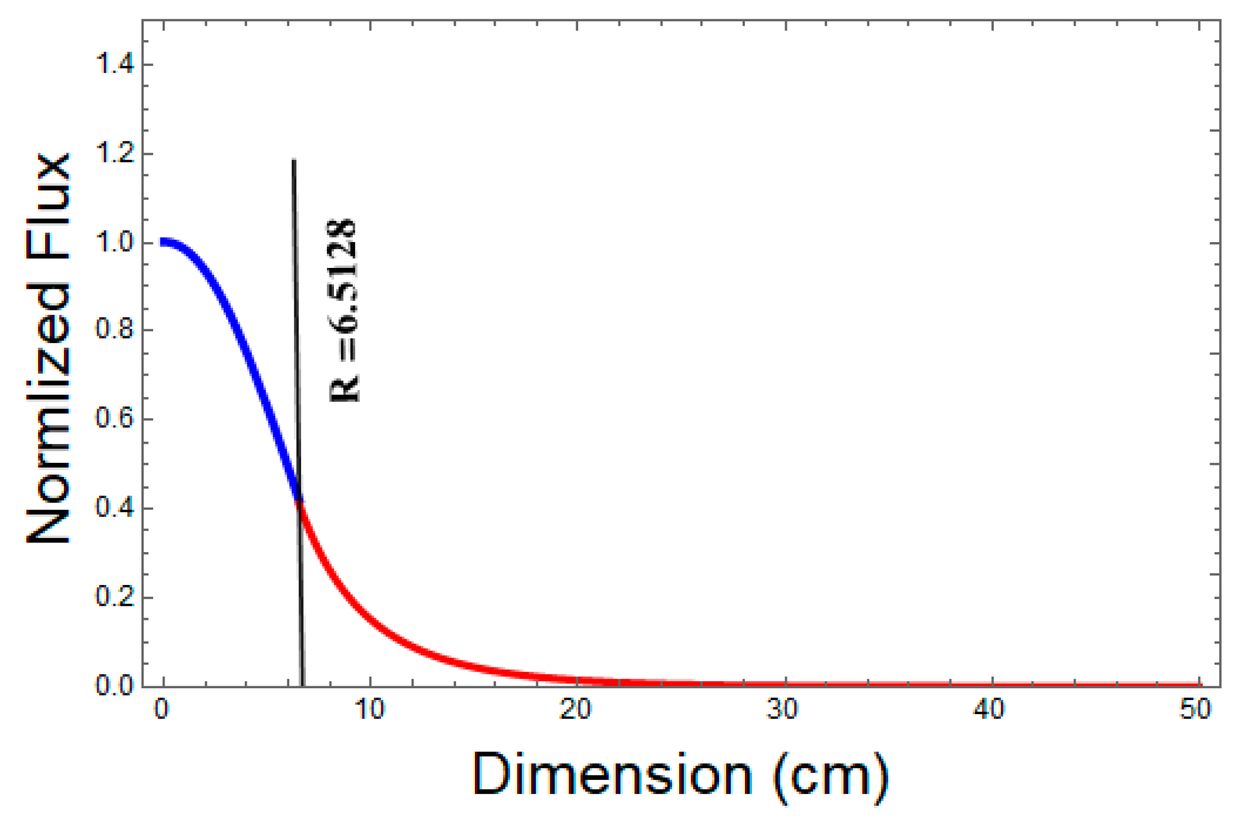
After finding the solution of neutron diffusion equations in the reactor core and reflector parts, it is essential to apply the boundary condition, the point , on the surface between them.
The neutron fluxes (
) must be continuous as well as their currents (
(
r)) [
24], which mathematically can be expressed as:
Neutron currents in Equation (38) will be defined as:
Therefore, after inserting the values of fluxes and currents in Equation (38), this system of equations can be written as:
By solving this system of equations computationally, we can find R.


