
A Discrete Dynamics Approach to a Tumor System

 , ,
, ,  ,
,
Abstract
:1. Introduction
2. The Continuous Version of the Cancer System
3. Discretization Methods
3.1. Euler Discretization Method
3.2. Taylor Series Expansion Method
3.3. Runge–Kutta Discretization Method
4. Stability Analysis for Discrete Cancer System
- If then , we have a saddle at this fixed point.
- If then , we have a node stable at this fixed point.
- (i)
- If , we have three real eigenvalues.
- (ii)
- If , we have one real and two complex eigenvalues that are stable with the selected parameter sets.
5. Chaotic Discrete Cancer System
- (1)
- All eigenvalues of the Jacobian of map (11) at the fixed point v are greater than the one with the Euclidean norm.
- (2)
- There exists and , such that, for all ,
- (1)
- F is continuously differentiable in the neighborhood of ; all the eigenvalues of have absolute values larger than 1, implying that there exists a positive constant r and a Euclidean norm, such that F expands in in the Euclidean norm, and
- (2)
- is a snap-back repeller of F with for some , and some positive integer m. Furthermore, F is continuously differentiable in some neighbourhoods of , respectively, and for , where .
A Proof of the Chaos of the Discrete Cancer System
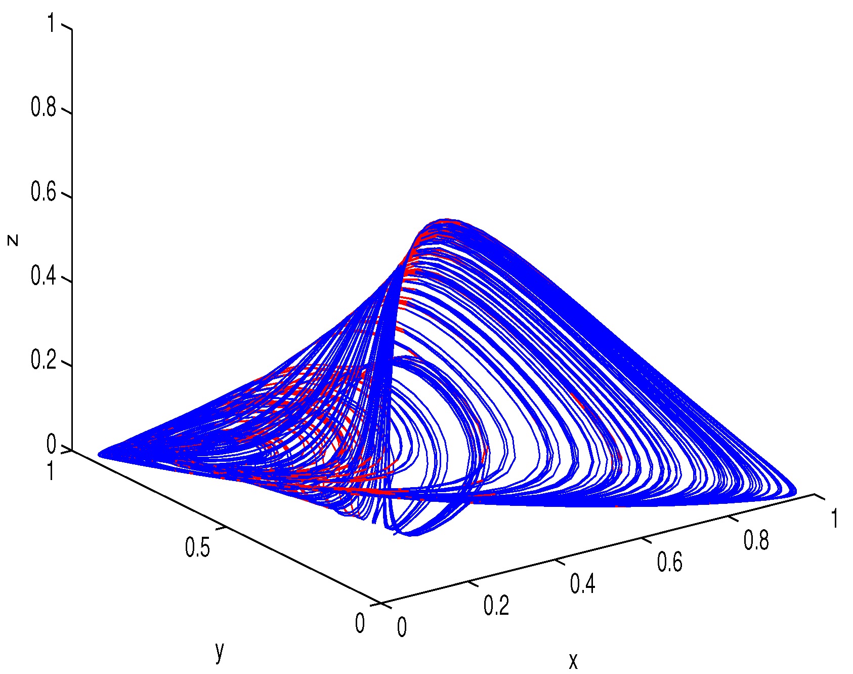
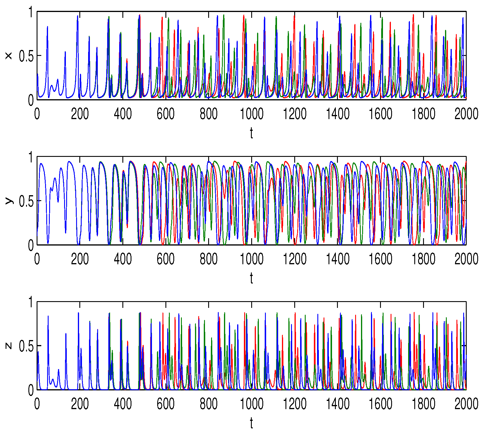
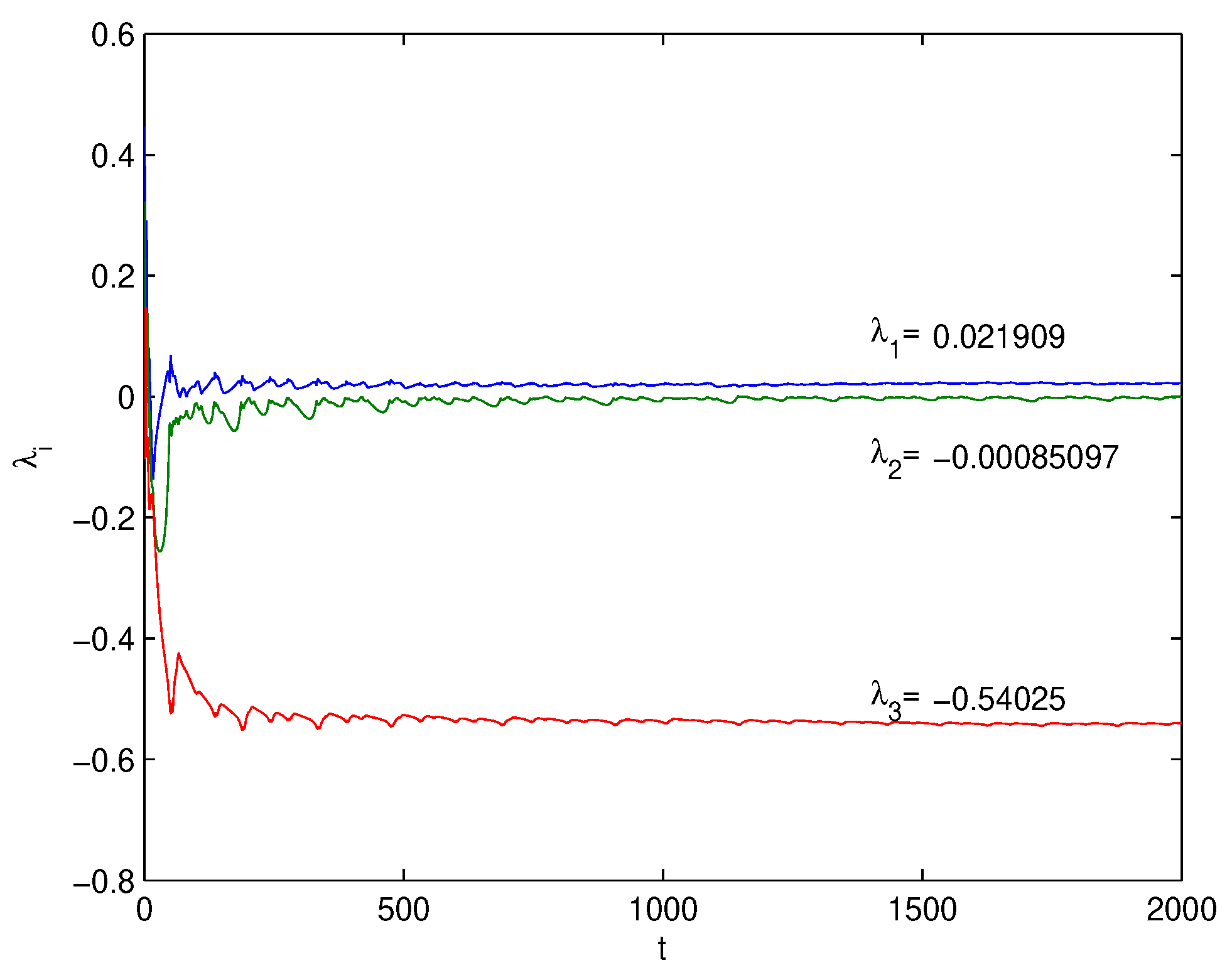
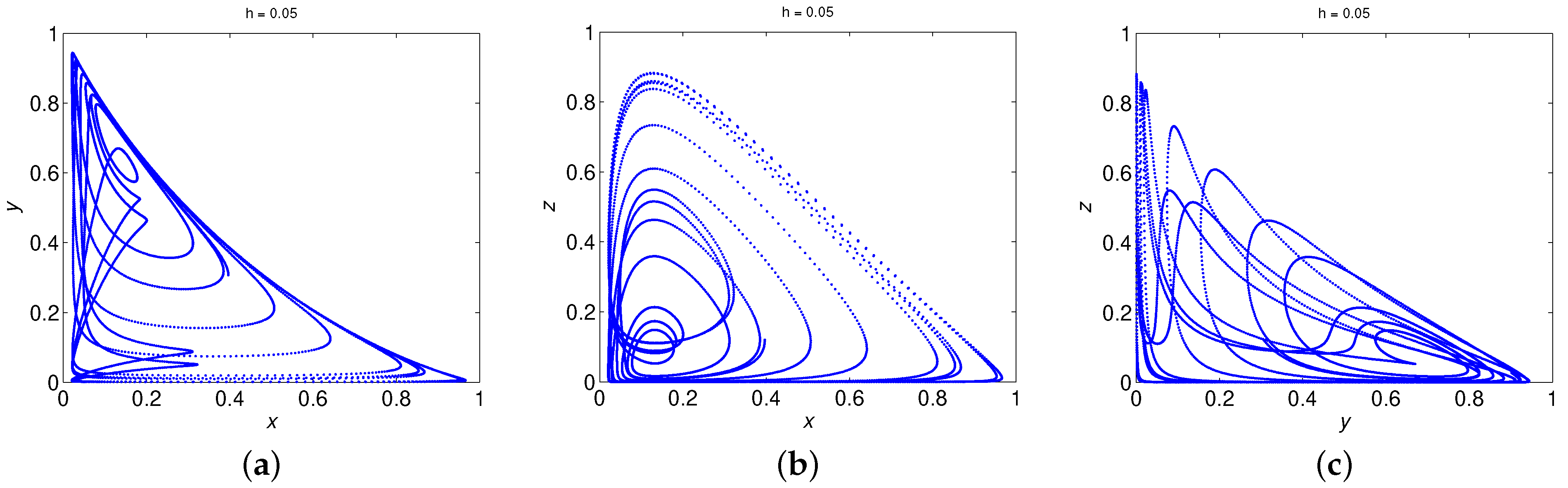
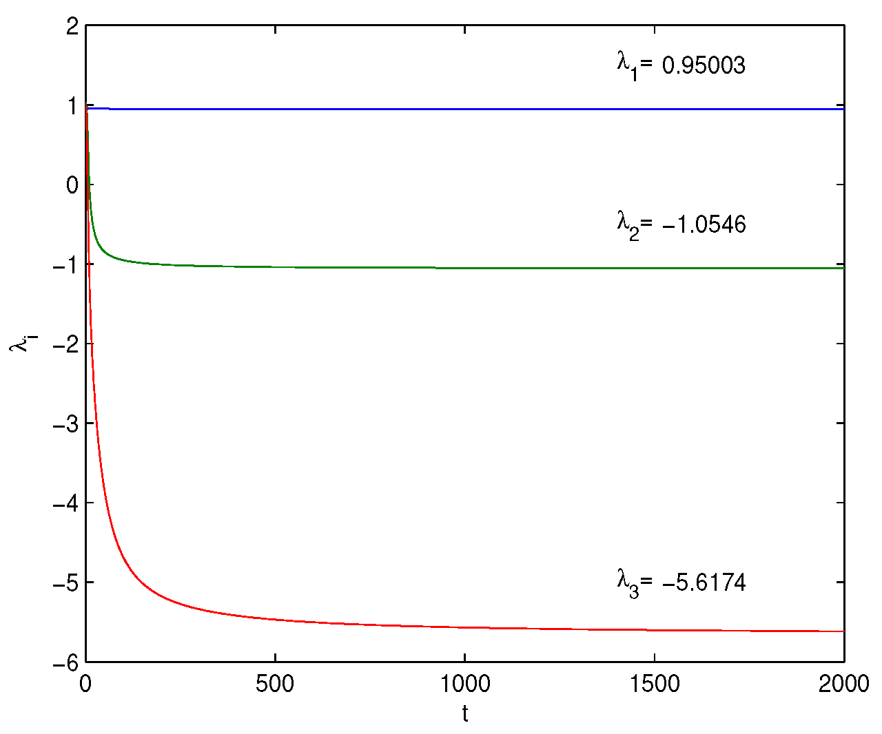
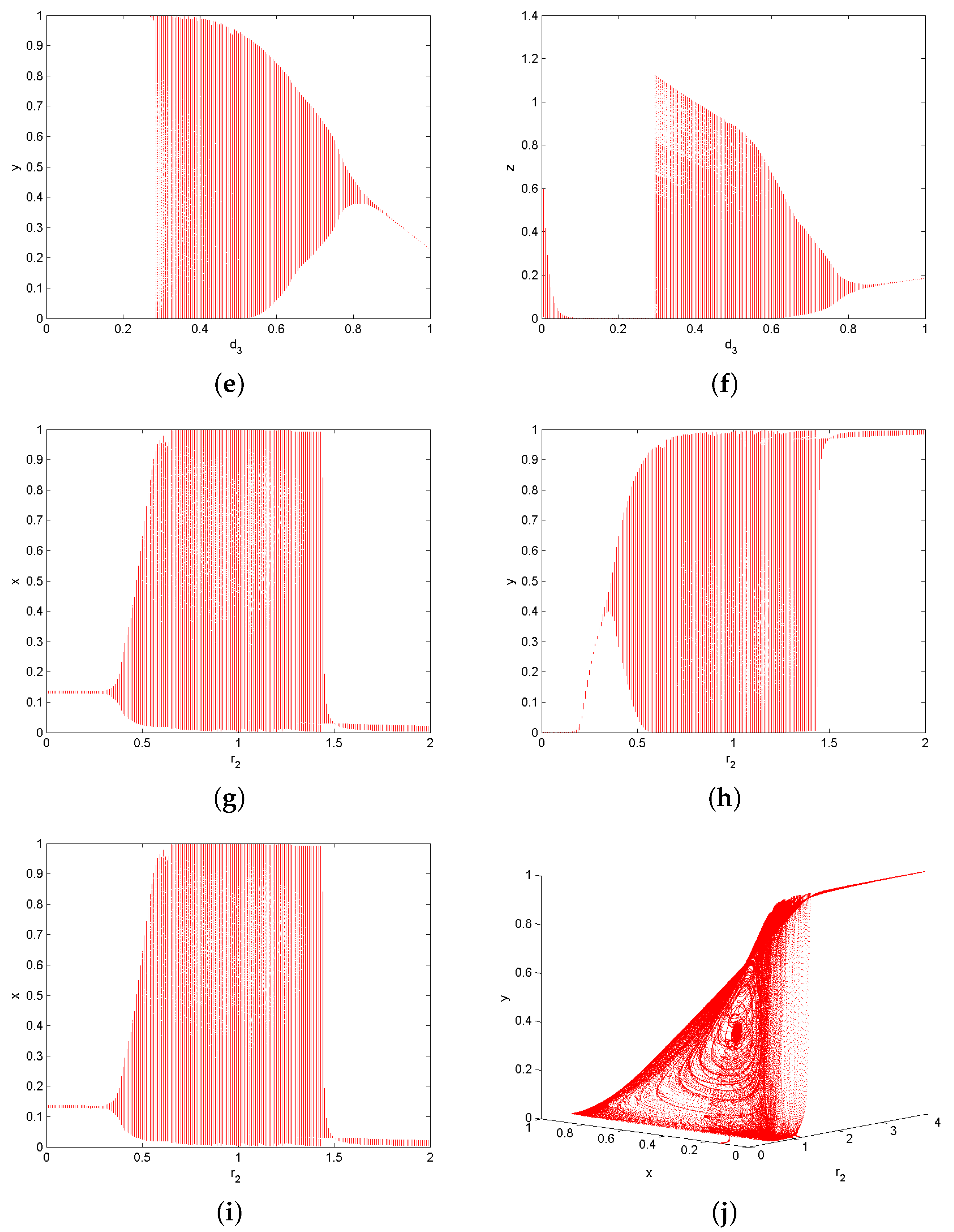
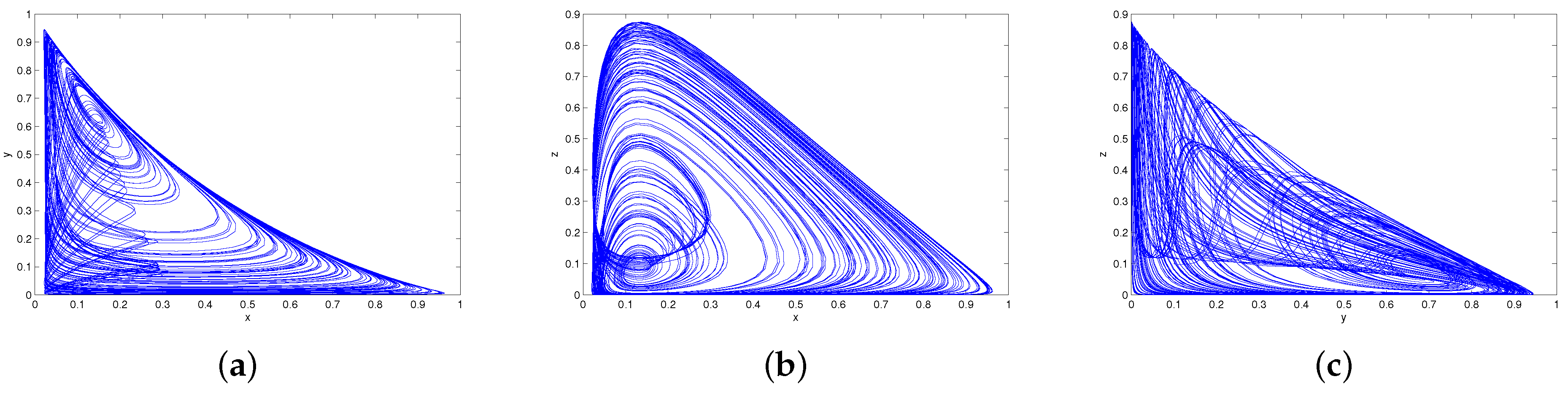
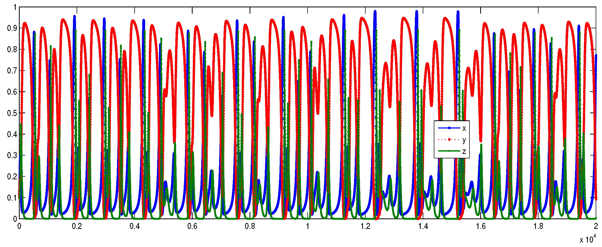
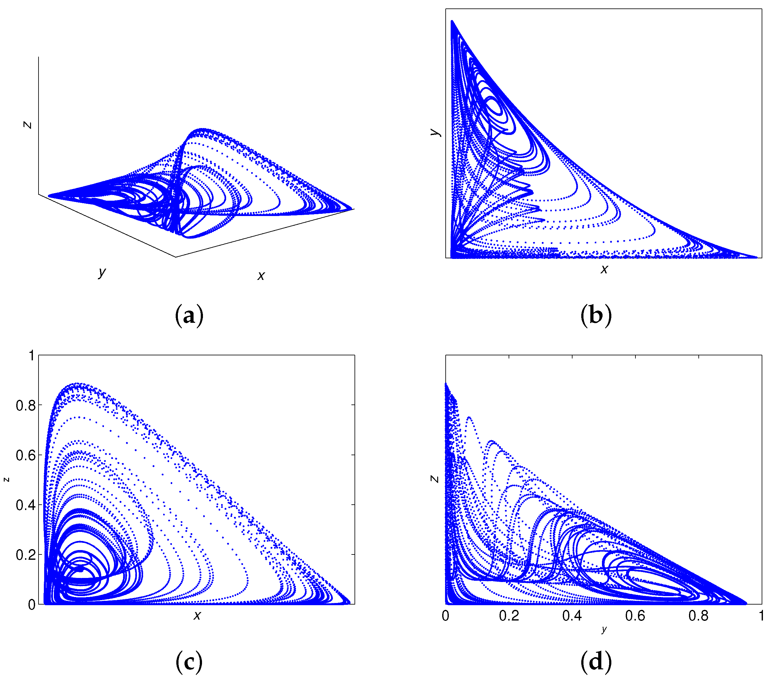
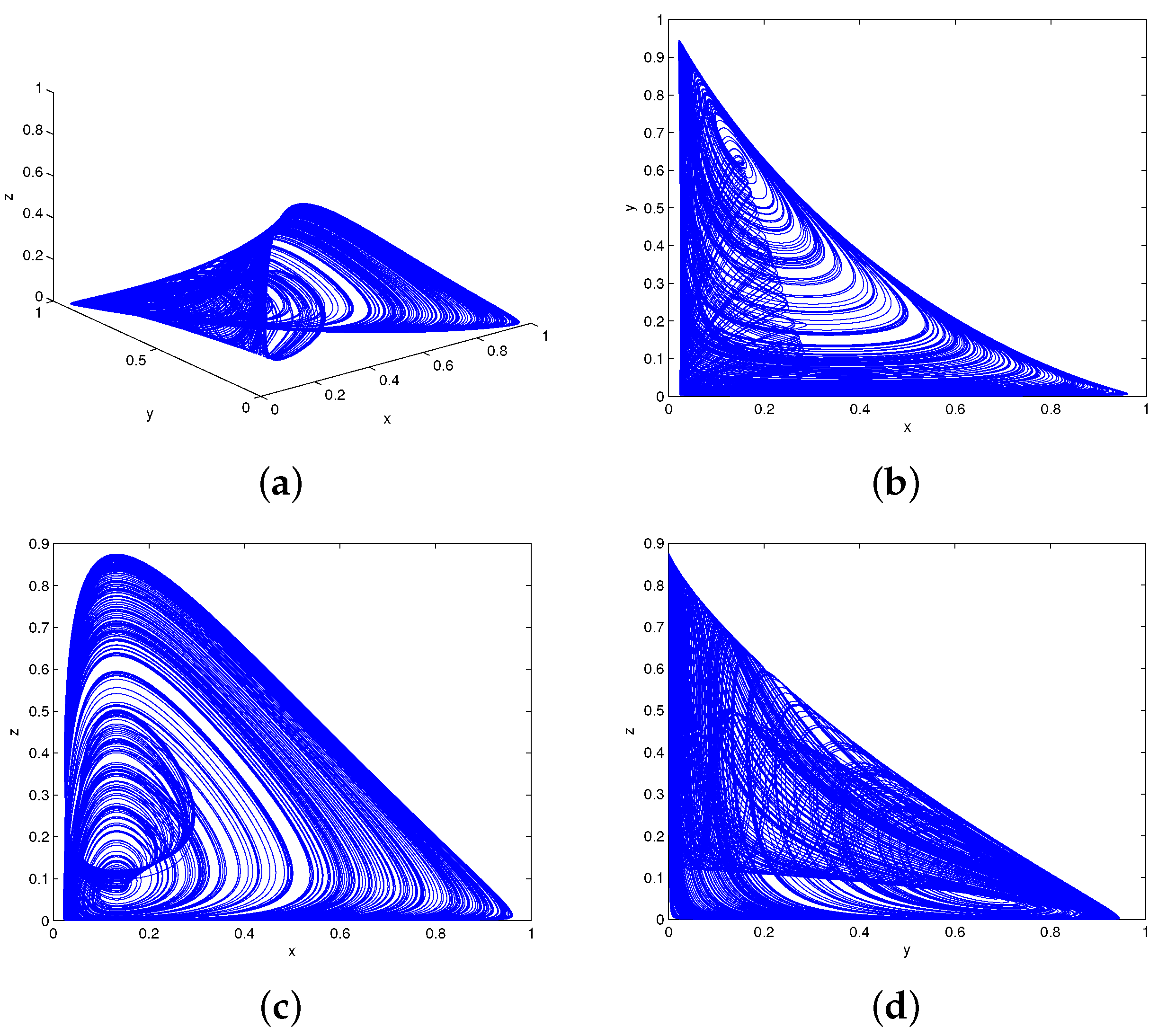
6. Numerical Simulations
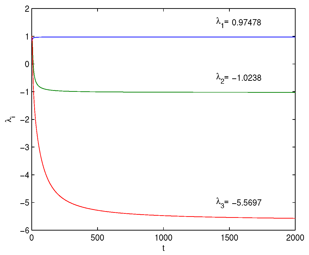
Lyapunov Exponents
7. Conclusions
Author Contributions
Funding
Data Availability Statement
Conflicts of Interest
References
- De Pillis, L.G.; Radunskaya, A. The dynamics of an optimally controlled tumor model: A case study. Math. Comput. 2003, 37, 1221–1244. [Google Scholar] [CrossRef]
- De Pillis, L.G.; Radunskaya, A.E.; Wiseman, C.L. A validated mathematical model of cell-mediated immune response to tumor growth. Cancer Res. 2005, 65, 7950–7958. [Google Scholar] [CrossRef] [PubMed] [Green Version]
- Eftimie, R.; Macnamara, C.K.; Dushoff, J.; Bramson, J.L.; Earn, D.J. Bifurcations and chaotic dynamics in a tumour-immune-virus system. Math. Model. Nat. 2016, 11, 65–85. [Google Scholar] [CrossRef] [Green Version]
- Kamel, D. Dynamics in a Discrete-Time Three Dimensional Cancer System. Int. J. Appl. Math. 2019, 49, 1–7. [Google Scholar]
- Karakaya, B.; Turk, M.A.; Turk, M.; Gulten, A. Selection of optimal numerical method for implementation of Lorenz Chaotic system on FPGA. Int. Res. Eng. J. 2018, 2, 147–152. [Google Scholar]
- Sarif Hassan, S. Computational Complex Dynamics Of The Discrete Lorenz System. arXiv 2016, arXiv:1604.02671. [Google Scholar]
- Selvam, A.G.; Roslin, D.; Rajendran, J. A discrete model of Rössler system. Int. J. Adv. Technol. Eng. Sci. 2014, 2, 130–134. [Google Scholar]
- Yuksel, G.; Isik, O.R. Numerical analysis of Backward-Euler discretization for simplified magnetohydrodynamic flows. Appl. Math. Model. 2015, 39, 1889–1898. [Google Scholar] [CrossRef]
- Song, W.; Liang, J. Difference equation of Lorenz system. Int. J. Pure Appl. Math. 2013, 83, 101–110. [Google Scholar]
- Zwarycz-Makles, K.; Majorkowska-Mech, D. Gear and Runge-Kutta Numerical Discretization Methods in Differential Equations of Adsorption in Adsorption Heat Pump. Appl. Sci. 2018, 8, 2437. [Google Scholar] [CrossRef] [Green Version]
- Murray, J.D. Mathematical biology I: An introduction. In Interdisciplinary Applied Mathematics, 3rd ed.; Springer: New York, NY, USA, 2002. [Google Scholar]
- Shi, Y.; Chen, G. Chaos of discrete dynamical systems in complete metric spaces. Chaos Solitons Fractals 2004, 22, 555–571. [Google Scholar] [CrossRef]
- Shi, Y.; Chen, G. Discrete chaos in Banach spaces. Sci. China Ser. A Math. 2005, 48, 222–238. [Google Scholar] [CrossRef]
- Wolf, A.; Swift, J.B.; Swinney, H.L.; Vastano, J.A. Determining Lyapunov exponents from a time series. Phys. D Nonlinear Phenom. 1985, 16, 285–317. [Google Scholar] [CrossRef] [Green Version]
- Pérez-García, V.M.; Fitzpatrick, S.; Pérez-Romasanta, L.A.; Pesic, M.; Schucht, P.; Arana, E.; Sánchez-Gómez, P. Applied mathematics and nonlinear sciences in the war on cancer. Appl. Math. Nonlinear Sci. 2016, 1, 423–436. [Google Scholar] [CrossRef] [Green Version]
- De Anda-Jáuregui, G.; Fresno, C.; García-Cortés, D.; Enríquez, J.E.; Hernández-Lemus, E. Intrachromosomal regulation decay in breast cancer. Appl. Math. Nonlinear Sci. 2019, 4, 223–230. [Google Scholar] [CrossRef] [Green Version]
- Amer, A.; Nagah, A.; Osman, M.A.-R.E.-N.; Majid, A. Modeling the pathway of breast cancer in the Middle East. Appl. Math. Nonlinear Sci. 2022. ahead of print. [Google Scholar] [CrossRef]


Publisher’s Note: MDPI stays neutral with regard to jurisdictional claims in published maps and institutional affiliations. |
© 2022 by the authors. Licensee MDPI, Basel, Switzerland. This article is an open access article distributed under the terms and conditions of the Creative Commons Attribution (CC BY) license (https://creativecommons.org/licenses/by/4.0/).
Share and Cite
Saeed, T.; Djeddi, K.; Guirao, J.L.G.; Alsulami, H.H.; Alhodaly, M.S. A Discrete Dynamics Approach to a Tumor System. Mathematics 2022, 10, 1774. https://doi.org/10.3390/math10101774
Saeed T, Djeddi K, Guirao JLG, Alsulami HH, Alhodaly MS. A Discrete Dynamics Approach to a Tumor System. Mathematics. 2022; 10(10):1774. https://doi.org/10.3390/math10101774
Chicago/Turabian StyleSaeed, Tareq, Kamel Djeddi, Juan L. G. Guirao, Hamed H. Alsulami, and Mohammed Sh. Alhodaly. 2022. "A Discrete Dynamics Approach to a Tumor System" Mathematics 10, no. 10: 1774. https://doi.org/10.3390/math10101774
APA StyleSaeed, T., Djeddi, K., Guirao, J. L. G., Alsulami, H. H., & Alhodaly, M. S. (2022). A Discrete Dynamics Approach to a Tumor System. Mathematics, 10(10), 1774. https://doi.org/10.3390/math10101774