
Scalable Visible Light Indoor Positioning System Using RSS

 , , ,
, , ,  , and
, and
Abstract
:1. Introduction
2. Materials
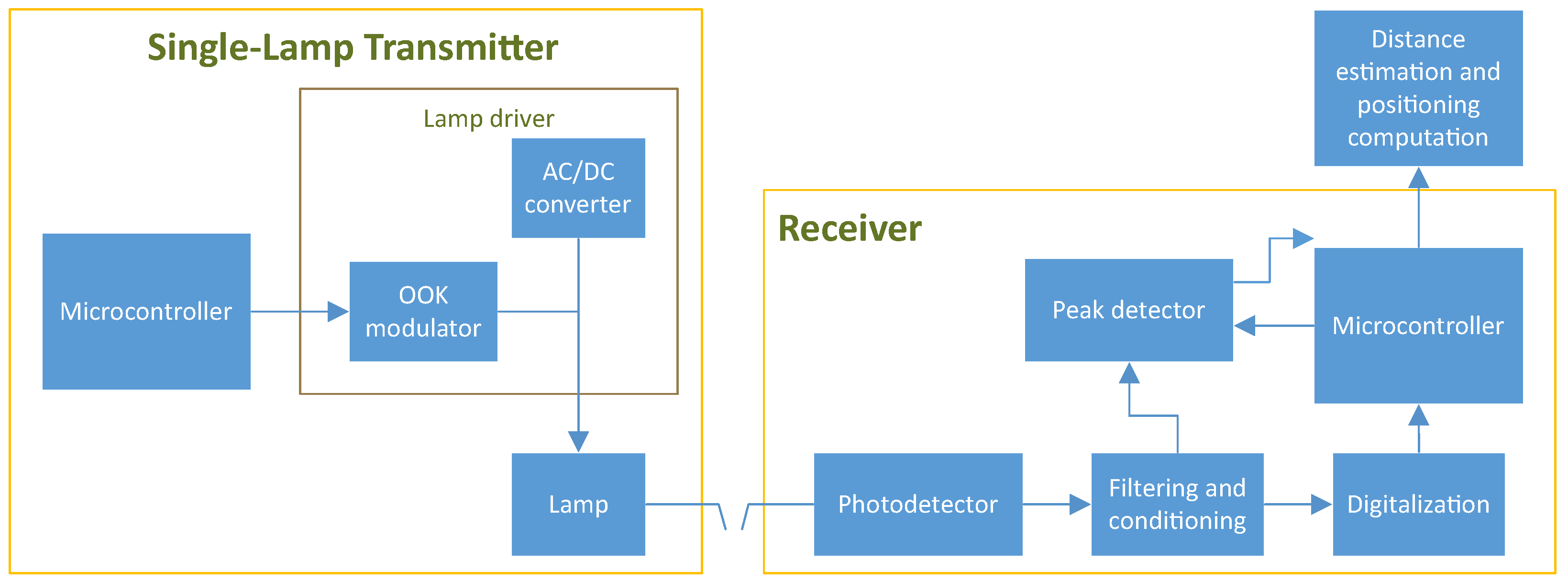
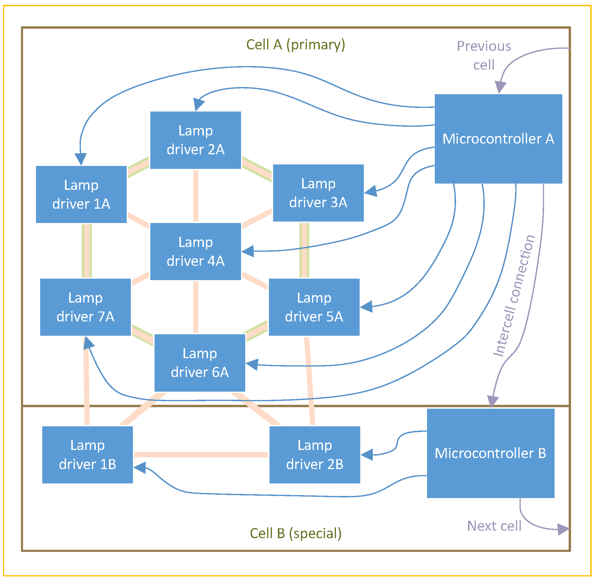
2.1. Transmitter
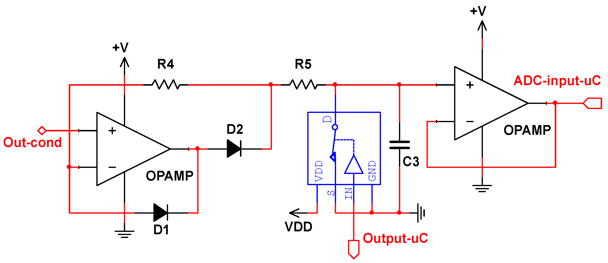
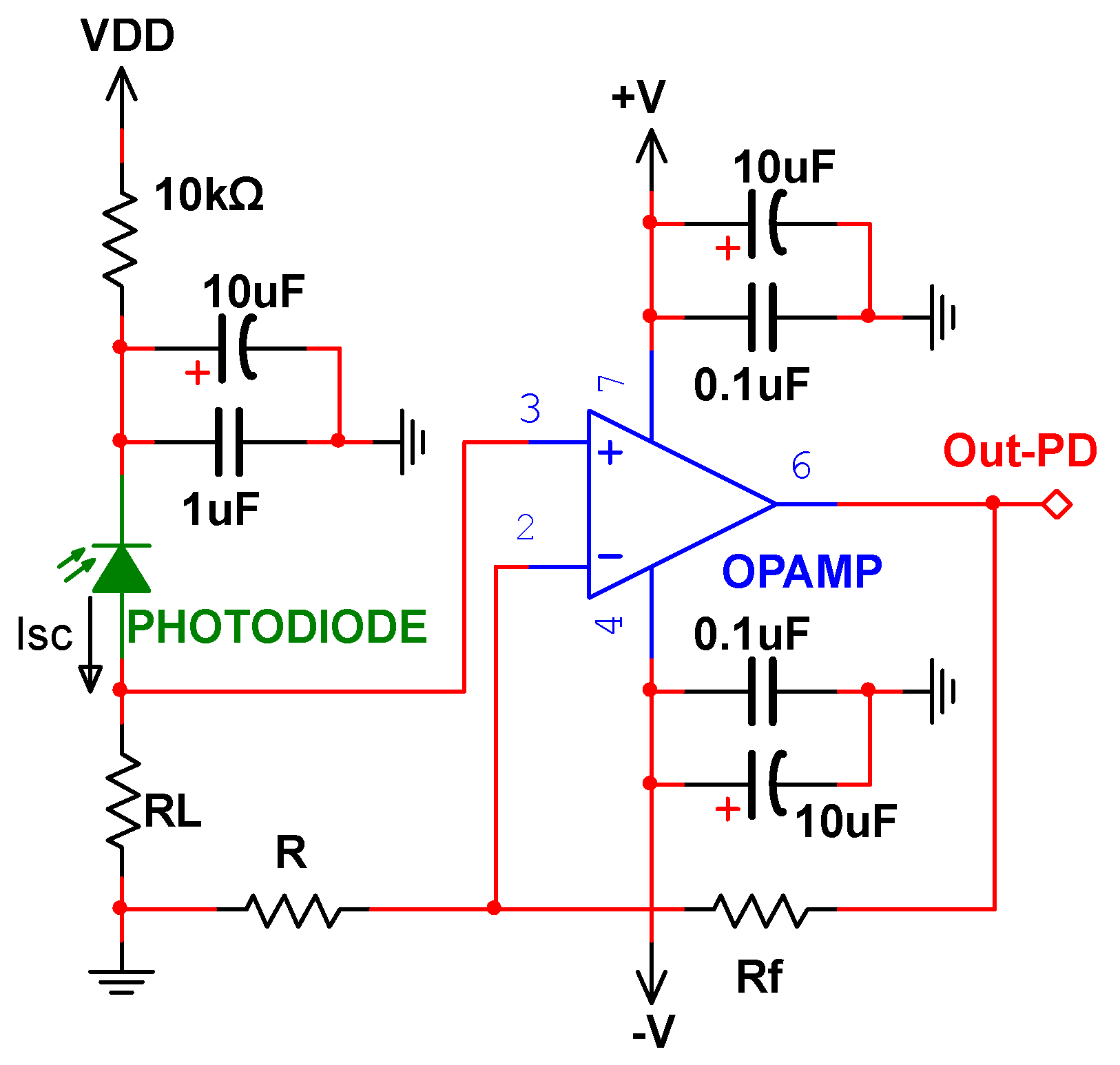
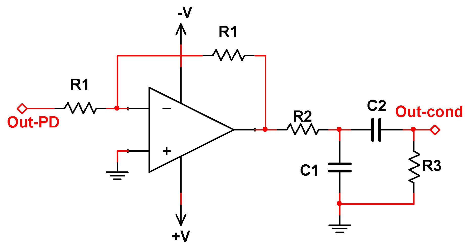
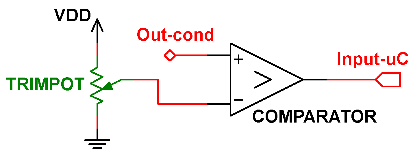
2.2. Receiver
3. Methods
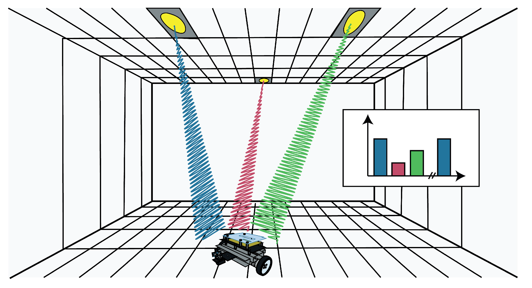
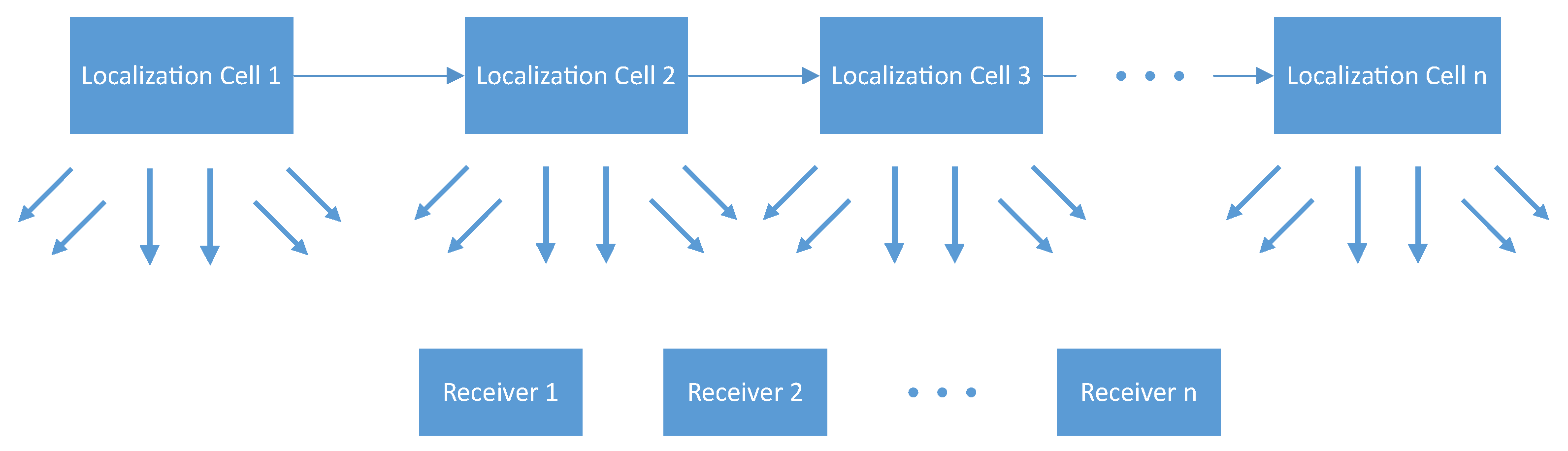
3.1. System Overview
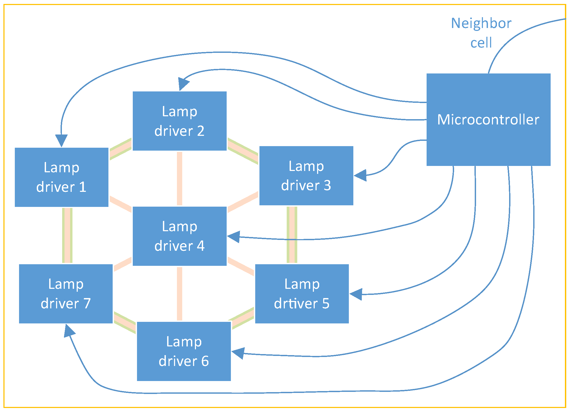
3.2. Medium Access Control
3.3. Synchronization
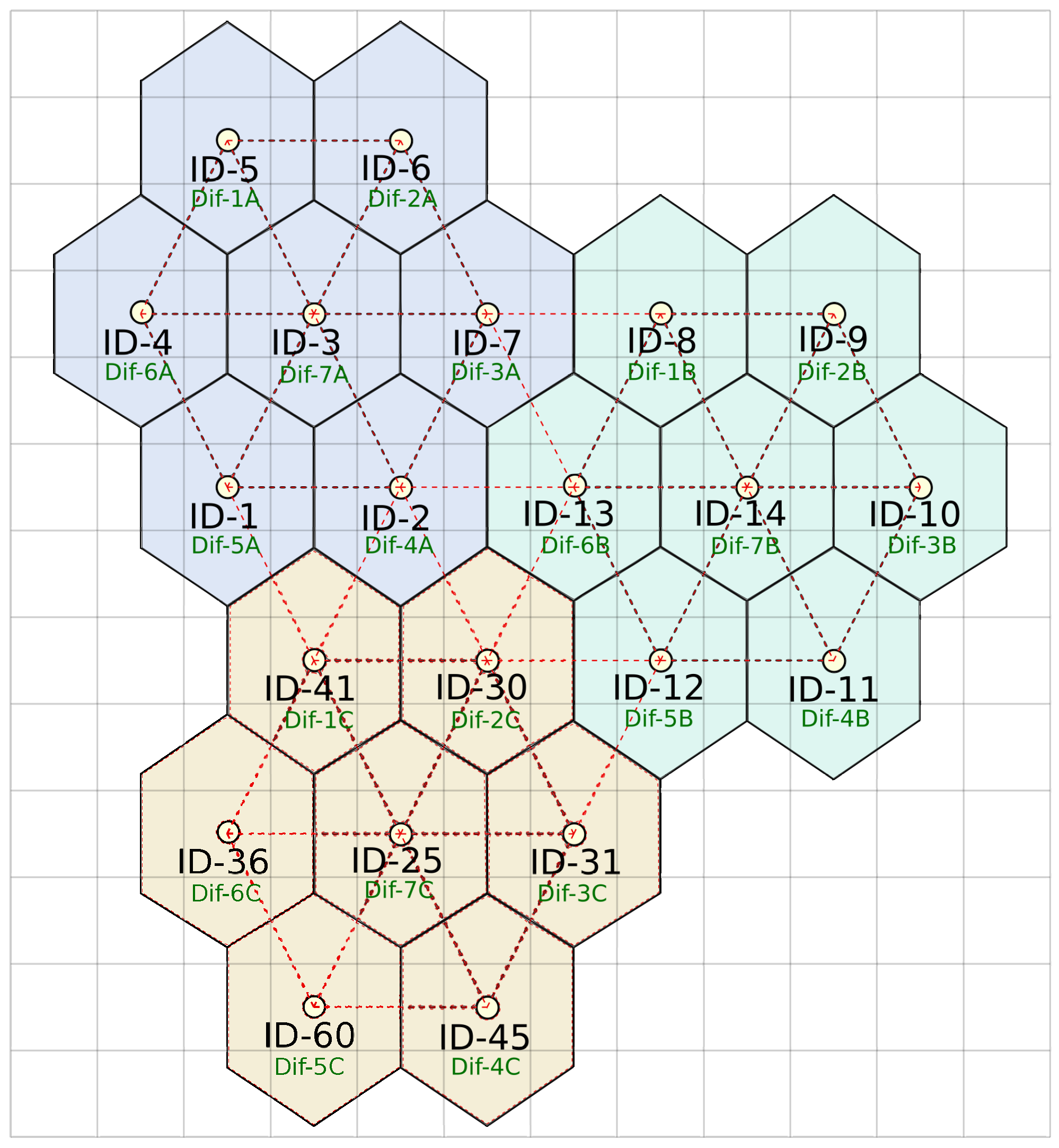
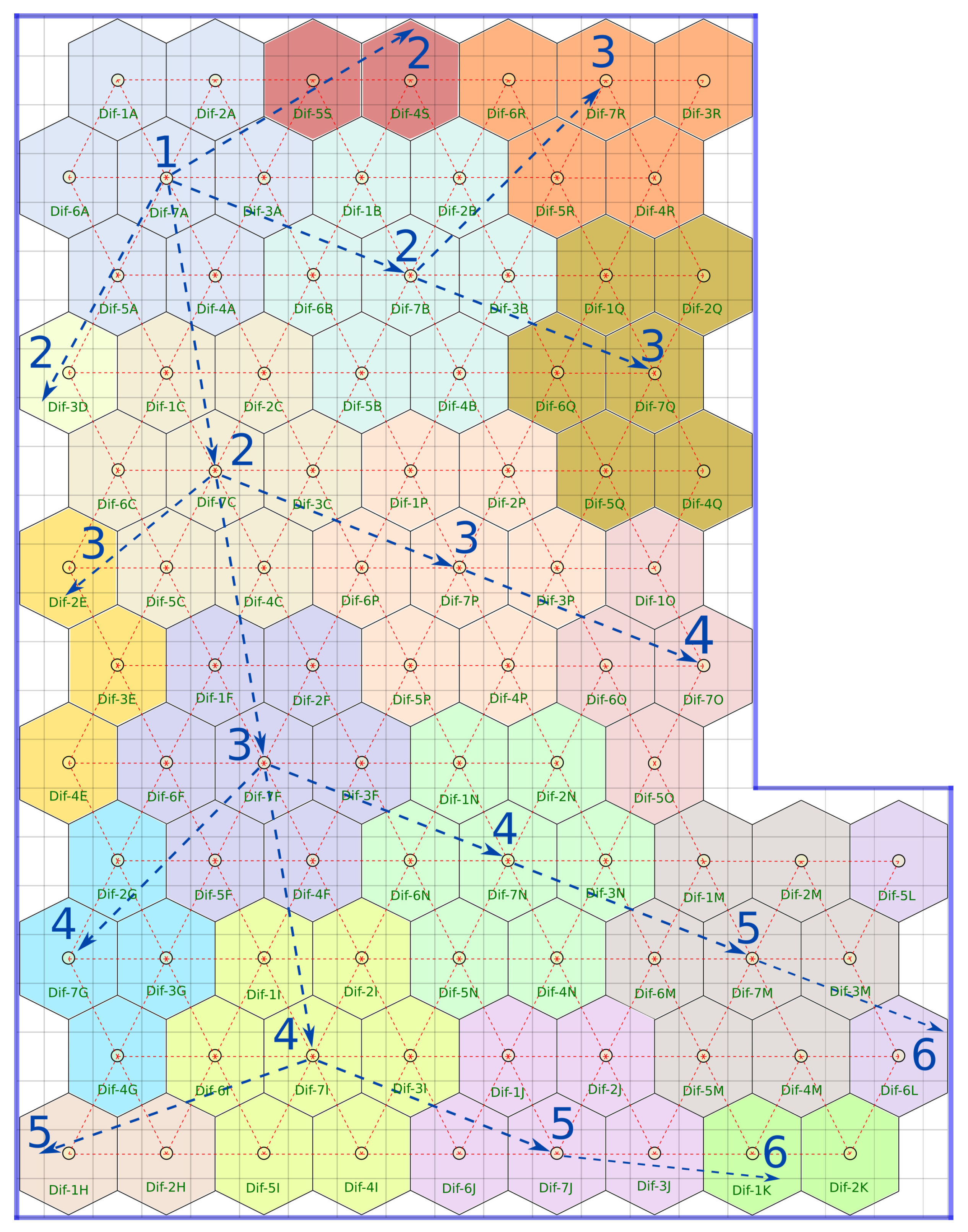
3.4. Deployment and Refresh Time
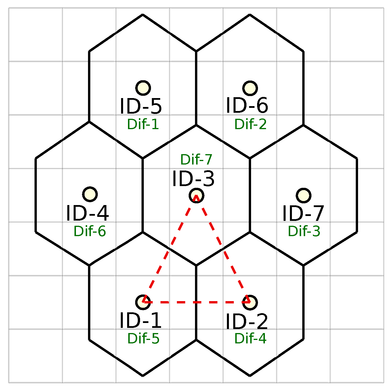
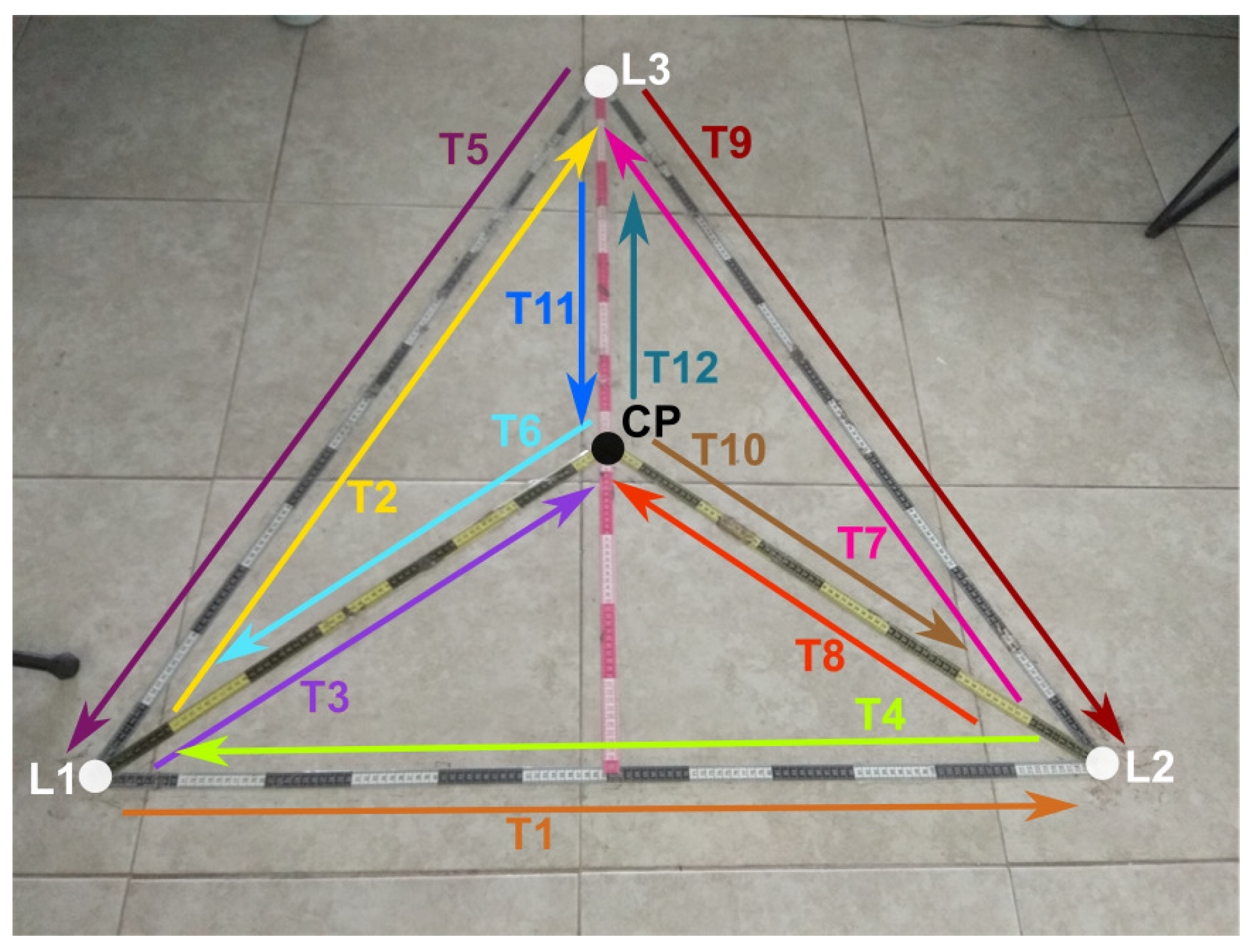
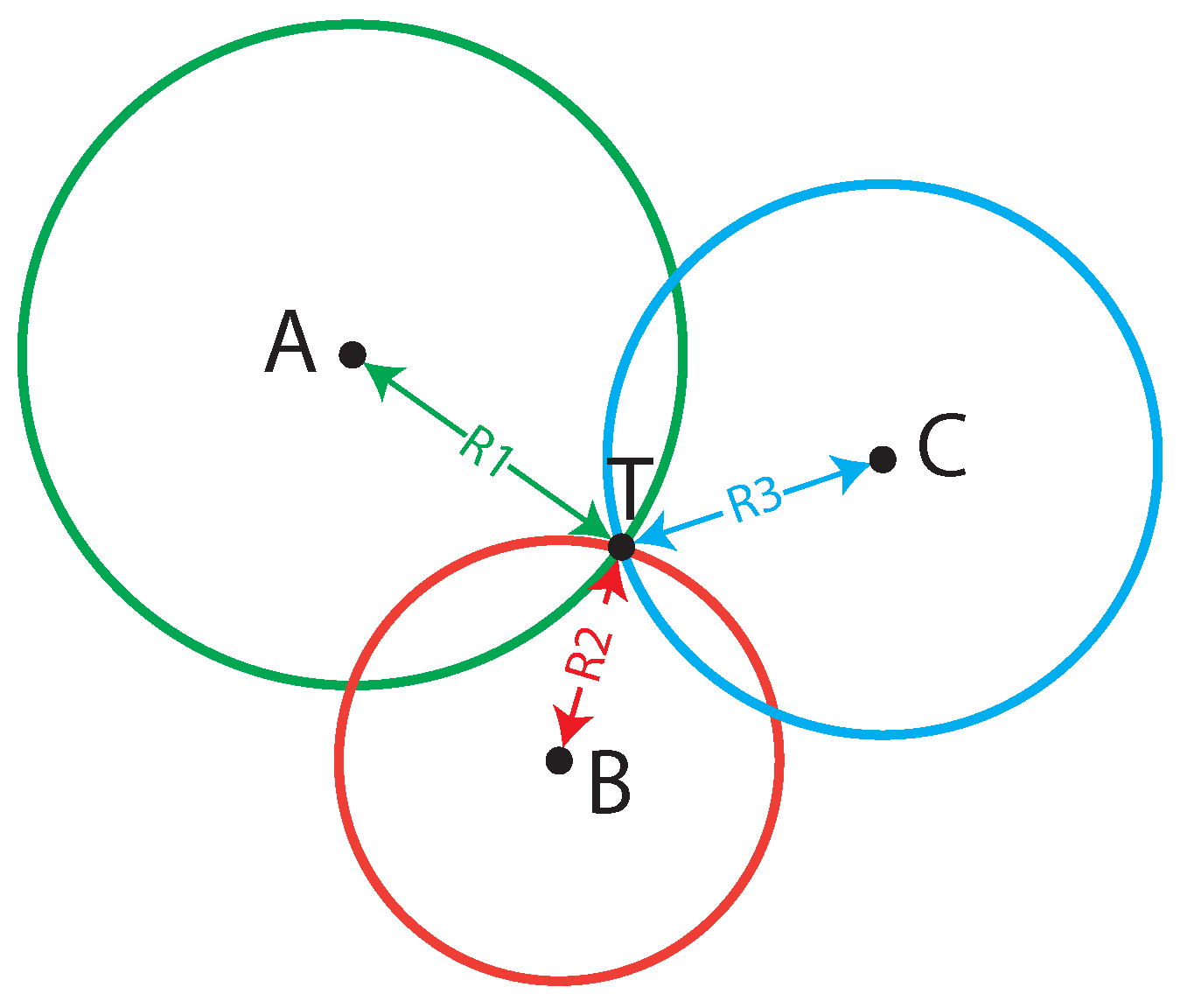
3.5. Localization Triangle
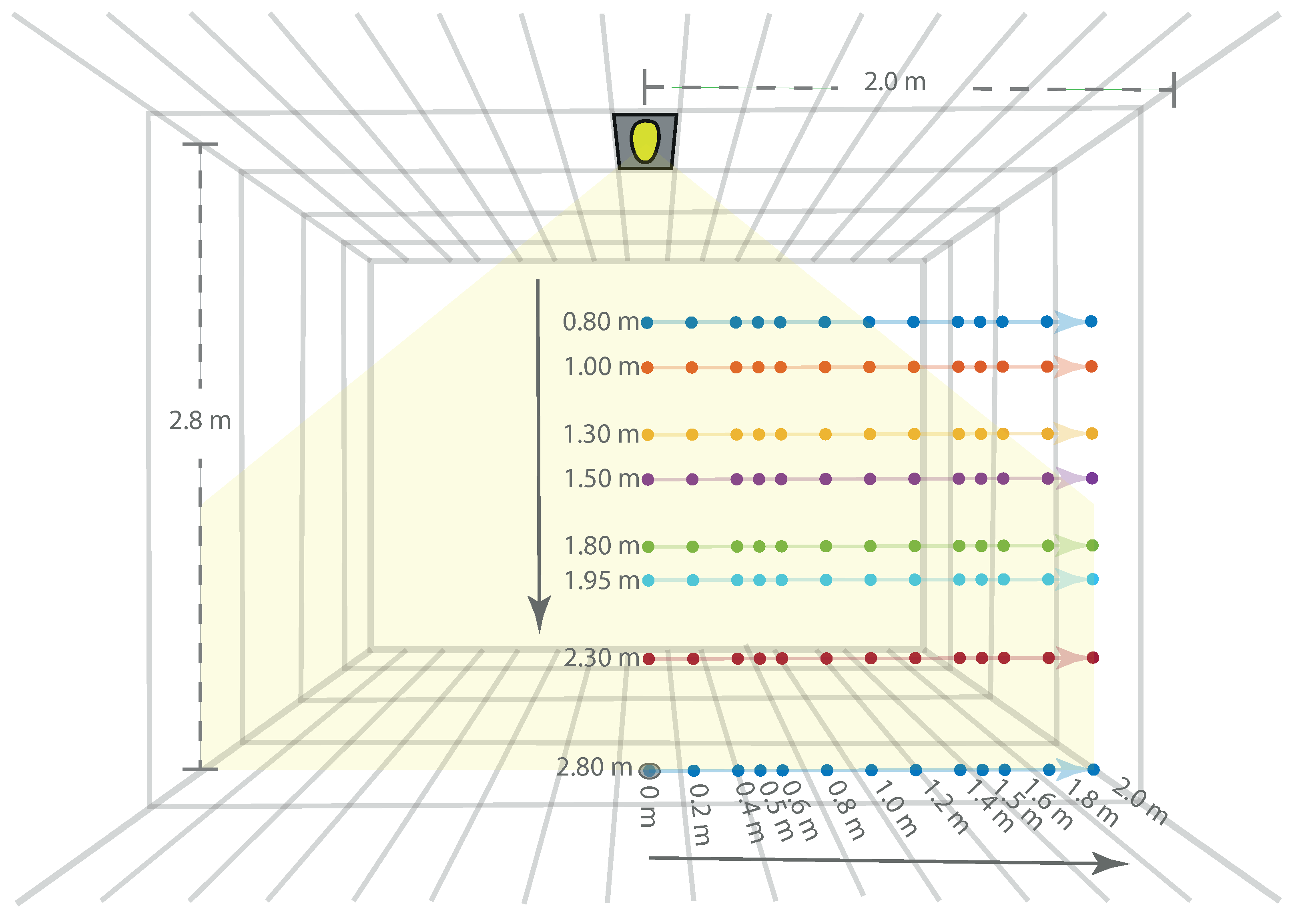
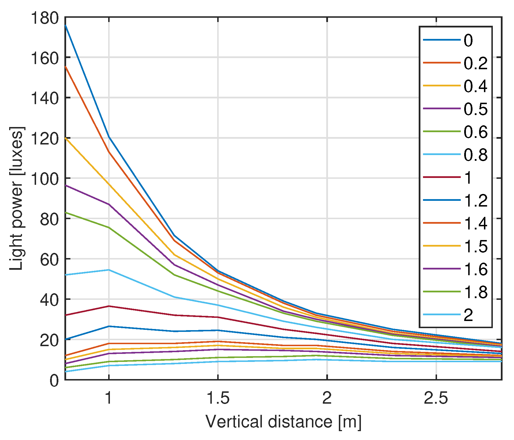
3.6. Distance Estimation
4. Results
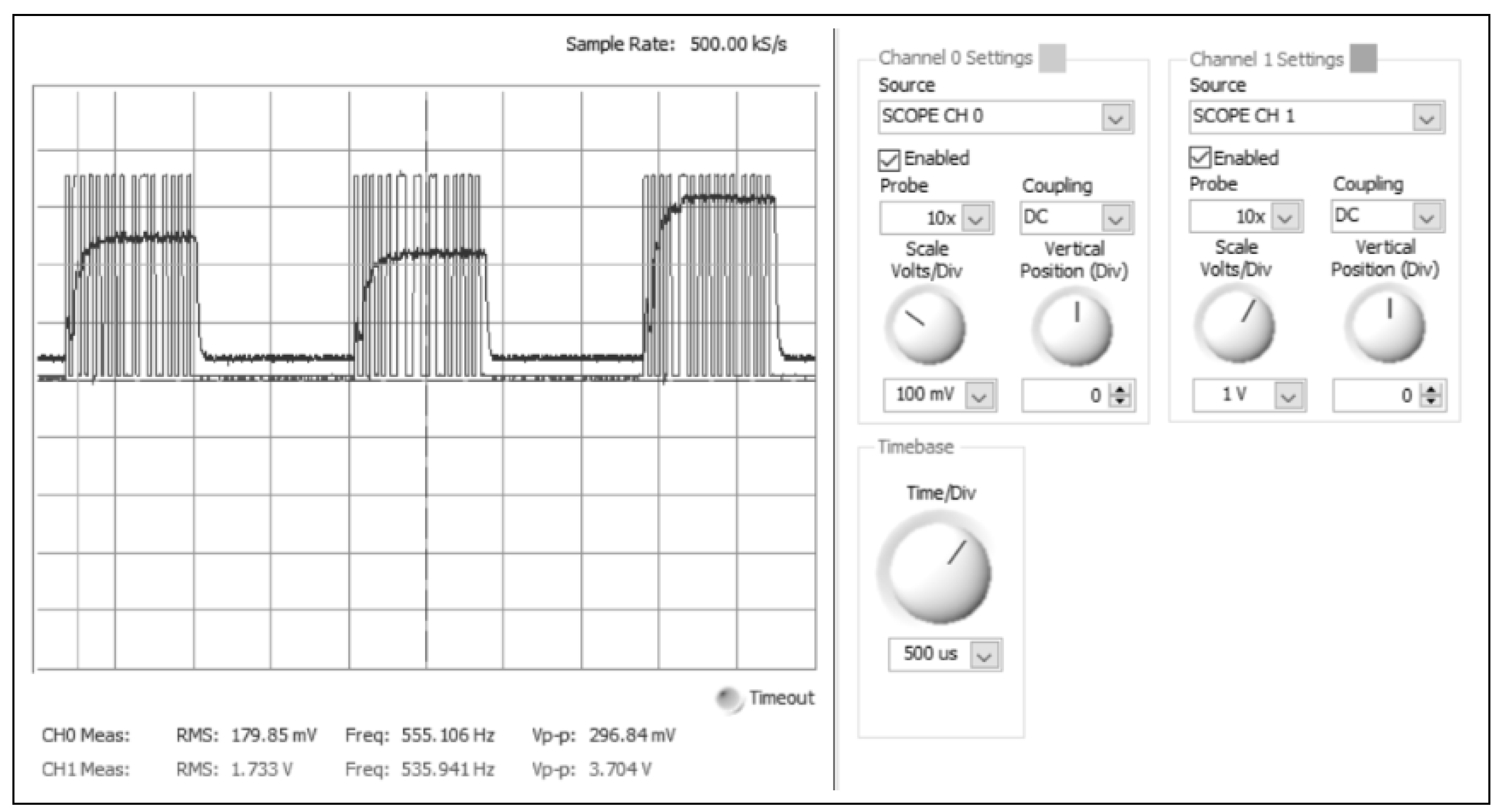
4.1. Transmitter
4.2. Receiver
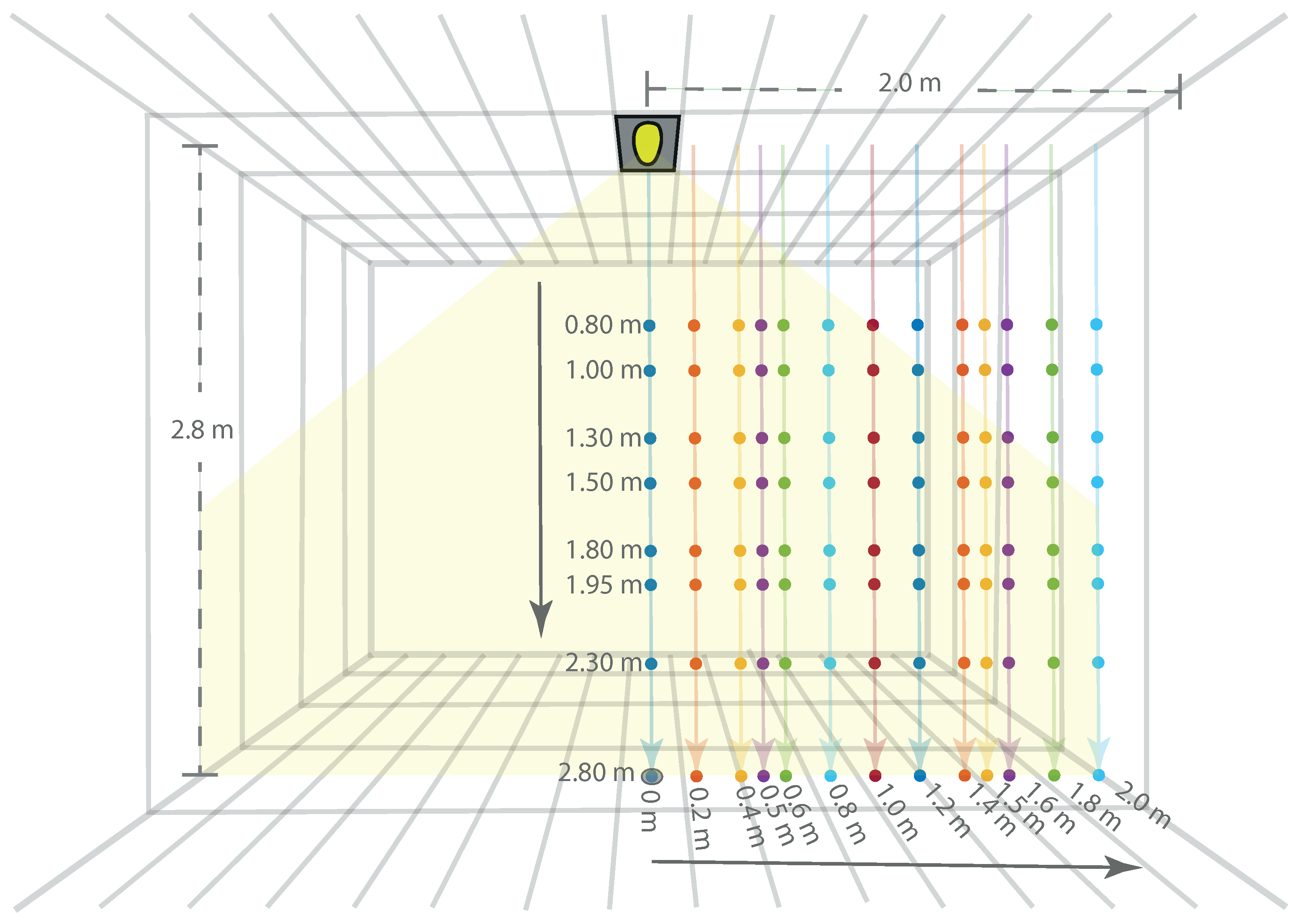
4.3. Test Scenario
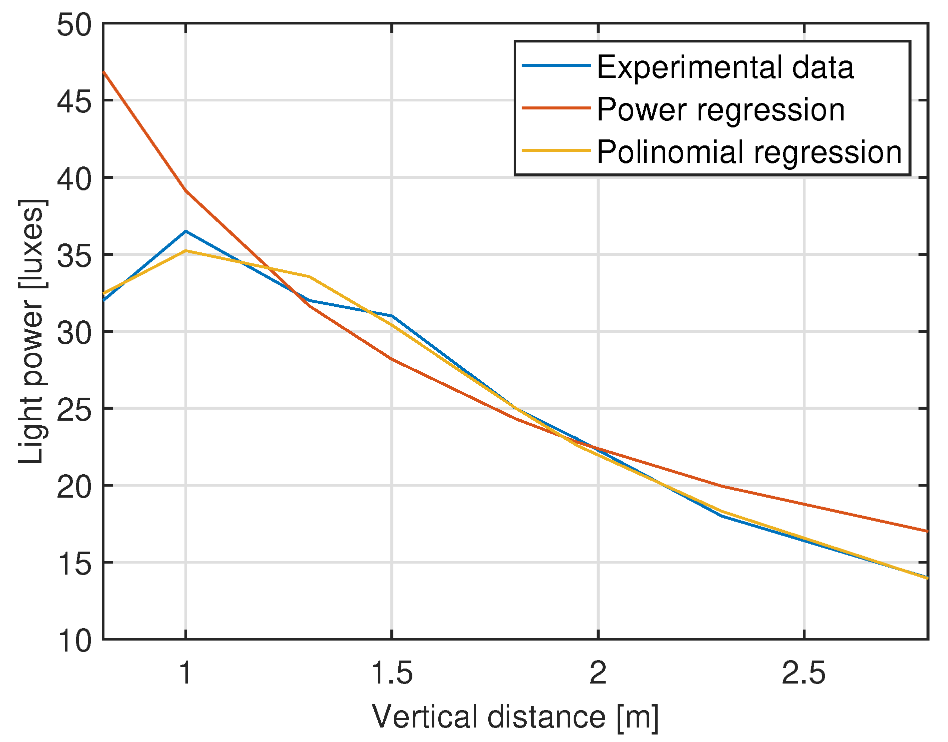
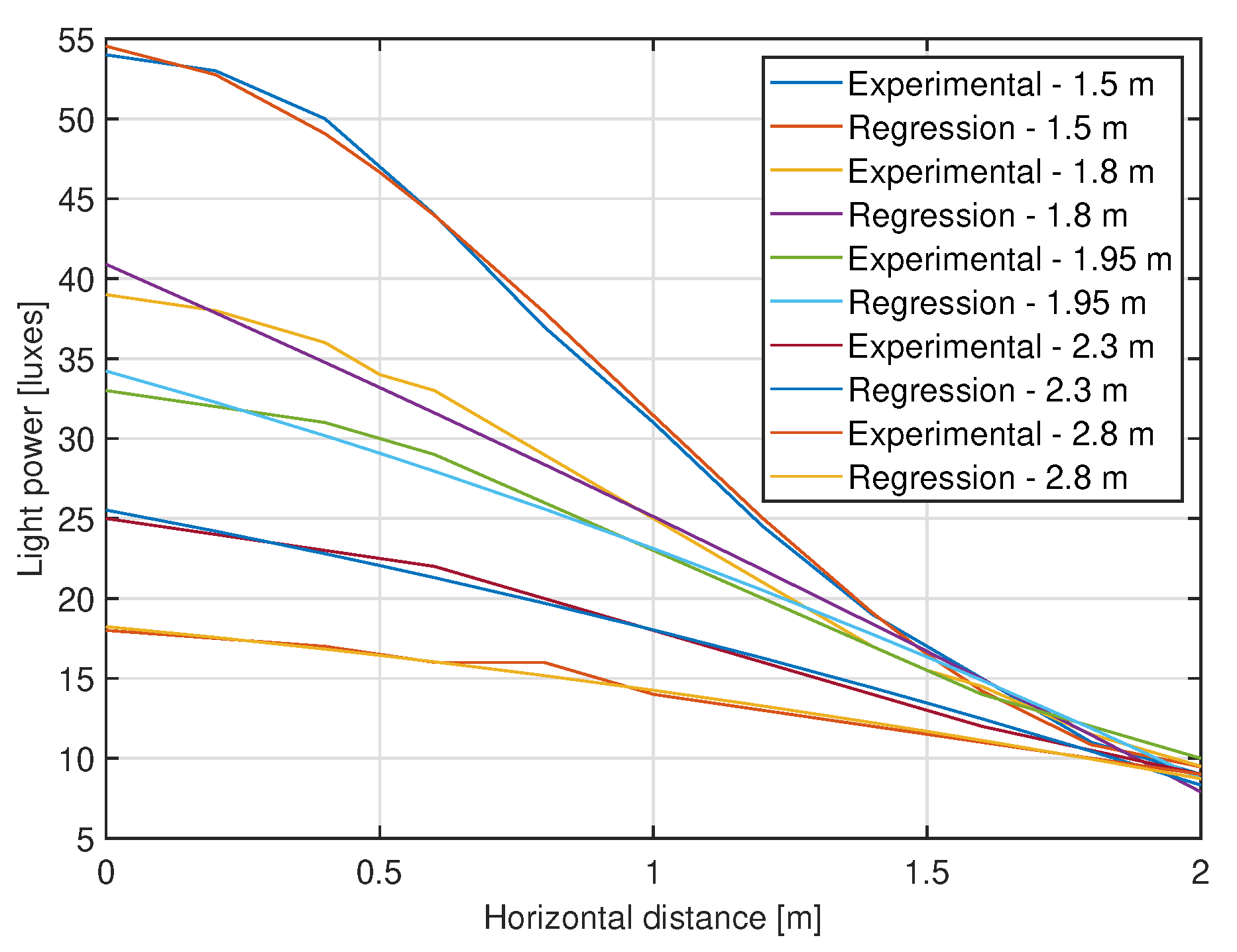
4.4. Distance Estimator
4.5. Experimental Results
5. Conclusions
Author Contributions
Funding
Institutional Review Board Statement
Informed Consent Statement
Data Availability Statement
Acknowledgments
Conflicts of Interest
Abbreviations
| LED | Light-Emitting Diode |
| IMDD | Intensity Modulation and Direct Detection |
| OKK | On–Off Keying |
| TDM | Time-Division Multiplexing |
| RSS | Received Signal Strength |
| ANN | Artificial Neural Network |
| IPS | Indoor Positioning System |
| RSS | Received Signal Strength |
| VLC | Visible Light Communications |
| VLPS | Visible Light Positioning System |
| GNSS | Global Navigation Satellite Systems |
| FoV | Field of View |
| IoT | Internet of Things |
| INS | Inertial Navigation System |
| WSN | Wireless Sensor Network |
| RF | Radio-Frequency |
| MLE | Maximum Likelihood Estimation |
| IM | Intensity Modulation |
| MOSFET | Metal-Oxide-Semiconductor Field-Effect Transistor |
| DC | Direct Current |
| MCU | Microcontroller |
| PD | Photodiode |
| DD | Direct Detection |
| SPST | Single Pole Single Throw |
| ADC | Analog to Digital Converter |
| S/H | Sampling and Hold |
| MAC | Medium Access Control |
| FDM | Frequency-Division Multiplexing |
| LOS | Line of Sight |
| MLP | Multi-Layer Perceptron |
References
- Department of Defense—United States of America and Navstar GPS. Global Positioning System Standard Positioning Service Performance Standard, 5th ed.; Department of Defense—United States of America and Navstar GPS: Arlington, VA, USA, 2020. [Google Scholar]
- Gu, Y.; Lo, A.; Niemegeers, I. A survey of indoor positioning systems for wireless personal networks. IEEE Commun. Surv. Tutor. 2009, 11, 13–32. [Google Scholar] [CrossRef] [Green Version]
- Koyuncu, H.; Yang, S.H. A survey of indoor positioning and object locating systems. IJCSNS Int. J. Comput. Sci. Netw. Secur. 2010, 10, 121–128. [Google Scholar]
- Mautz, R.; Tilch, S. Survey of optical indoor positioning systems. In Proceedings of the 2011 International Conference on Indoor Positioning and Indoor Navigation, Guimaraes, Portugal, 21–23 September 2011; pp. 1–7. [Google Scholar]
- Nuaimi, K.A.; Kamel, H. A Survey of Indoor Positioning Systems and Algorithms. In Proceedings of the 2011 International Conference on Innovations in Information Technology (IIT), Abu Dhabi, United Arab Emirates, 25–27 April 2011; pp. 185–190. [Google Scholar] [CrossRef]
- IEEE Std 802.15.7-2011; IEEE Standard for Local and Metropolitan Area Networks–Part 15.7: Short-Range Wireless Optical Communication Using Visible Light. IEEE: Piscataway, NJ, USA, 2011; pp. 1–309. [CrossRef]
- Dardari, D.; Closas, P.; Djurić, P.M. Indoor Tracking: Theory, Methods, and Technologies. IEEE Trans. Veh. Technol. 2015, 64, 1263–1278. [Google Scholar] [CrossRef] [Green Version]
- Zhuang, Y.; Hua, L.; Qi, L.; Yang, J.; Cao, P.; Cao, Y.; Wu, Y.; Thompson, J.; Haas, H. A Survey of Positioning Systems Using Visible LED Lights. IEEE Commun. Surv. Tutor. 2018, 20, 1963–1988. [Google Scholar] [CrossRef] [Green Version]
- Yu, N.; Wang, S. Enhanced Autonomous Exploration and Mapping of an Unknown Environment with the Fusion of Dual RGB-D Sensors. Engineering 2019, 5, 164–172. [Google Scholar] [CrossRef]
- Chen, X.C.; Chu, S.; Li, F.; Chu, G. Hybrid ToA and IMU indoor localization system by various algorithms. J. Cent. South Univ. 2019, 26, 2281–2294. [Google Scholar] [CrossRef]
- Dong, L.; Sun, D.; Han, G.; Li, X.; Hu, Q.; Shu, L. Velocity-Free Localization of Autonomous Driverless Vehicles in Underground Intelligent Mines. IEEE Trans. Veh. Technol. 2020, 69, 9292–9303. [Google Scholar] [CrossRef]
- Gubbi, J.; Buyya, R.; Marusic, S.; Palaniswami, M. Internet of Things (IoT): A vision, architectural elements, and future directions. Future Gener. Comput. Syst. 2013, 29, 1645–1660. [Google Scholar] [CrossRef] [Green Version]
- Shaikh, F.K.; Zeadally, S. Energy harvesting in wireless sensor networks: A comprehensive review. Renew. Sustain. Energy Rev. 2016, 55, 1041–1054. [Google Scholar] [CrossRef]
- Hui, T.K.L.; Sherratt, R.S.; Sánchez, D.D. Major requirements for building Smart Homes in Smart Cities based on Internet of Things technologies. Future Gener. Comput. Syst. 2017, 76, 358–369. [Google Scholar] [CrossRef] [Green Version]
- Elgala, H.; Mesleh, R.; Haas, H. Indoor optical wireless communication: Potential and state-of-the-art. IEEE Commun. Mag. 2011, 49, 56–62. [Google Scholar] [CrossRef]
- Haas, H.; Yin, L.; Wang, Y.; Chen, C. What is LiFi? J. Light. Technol. 2016, 34, 1533–1544. [Google Scholar] [CrossRef]
- Mousa, F.I.K.; Almaadeed, N.; Busawon, K.; Bouridane, A.; Binns, R.; Elliott, I. Indoor visible light communication localization system utilizing received signal strength indication technique and trilateration method. Opt. Eng. 2018, 57, 016107. [Google Scholar] [CrossRef]
- Avendaño-Lopez, C.M. Diseño e Implementacion de un Sistema de Posicionamiento en Ambientes de Interiores Basados en VLC. Ph.D. Thesis, Universidad de Guanajuato Campus Irapuato-Salamanca División de Ingenierías, Salamanca, Mexico, 2018. [Google Scholar]
- Avendaño López, C.M.; Ibarra-Manzano, M.A.; Castro-Sánchez, R.; Almanza-Ojeda, D.L.; Gómez-Carranza, J.C.; Amézquita Sánchez, J.P.; Rivera Guillen, J.R.; Rangel Magdaleno, J.D.J. Indoor Positioning System Based on Visible Light Communications. In Proceedings of the 2018 International Conference on Mechatronics, Electronics and Automotive Engineering (ICMEAE), Cuernavaca, Mexico, 27–30 November 2018; pp. 26–31. [Google Scholar] [CrossRef]
- Kim, H.S.; Kim, D.R.; Yang, S.H.; Son, Y.H.; Han, S.K. An Indoor Visible Light Communication Positioning System Using a RF Carrier Allocation Technique. J. Light. Technol. 2013, 31, 134–144. [Google Scholar] [CrossRef]
- Lee, K.; Park, H.; Barry, J.R. Indoor Channel Characteristics for Visible Light Communications. IEEE Commun. Lett. 2011, 15, 217–219. [Google Scholar] [CrossRef]


| Model | Mean Absolute Error | Standard Deviation |
|---|---|---|
| Quadratic | 2.40 cm | 1.90 cm |
| Individual ANN | 2.50 cm | 1.60 cm |
| General ANN | 39.8 cm | 30.1 cm |
| Model | MSE | RMSE |
|---|---|---|
| Quadratic | 0.0976 mm | 3.10 cm |
| Individual ANN | 0.0897 mm | 3.00 cm |
| General ANN | 0.0868 mm | 9.30 cm |
Publisher’s Note: MDPI stays neutral with regard to jurisdictional claims in published maps and institutional affiliations. |
© 2022 by the authors. Licensee MDPI, Basel, Switzerland. This article is an open access article distributed under the terms and conditions of the Creative Commons Attribution (CC BY) license (https://creativecommons.org/licenses/by/4.0/).
Share and Cite
Avendaño-Lopez, C.M.; Castro-Sanchez, R.; Almanza-Ojeda, D.L.; Avina-Cervantes, J.G.; Gomez-Martinez, M.A.; Ibarra-Manzano, M.A. Scalable Visible Light Indoor Positioning System Using RSS. Mathematics 2022, 10, 1738. https://doi.org/10.3390/math10101738
Avendaño-Lopez CM, Castro-Sanchez R, Almanza-Ojeda DL, Avina-Cervantes JG, Gomez-Martinez MA, Ibarra-Manzano MA. Scalable Visible Light Indoor Positioning System Using RSS. Mathematics. 2022; 10(10):1738. https://doi.org/10.3390/math10101738
Chicago/Turabian StyleAvendaño-Lopez, Carlos M., Rogelio Castro-Sanchez, Dora L. Almanza-Ojeda, Juan Gabriel Avina-Cervantes, Miguel A. Gomez-Martinez, and Mario A. Ibarra-Manzano. 2022. "Scalable Visible Light Indoor Positioning System Using RSS" Mathematics 10, no. 10: 1738. https://doi.org/10.3390/math10101738
APA StyleAvendaño-Lopez, C. M., Castro-Sanchez, R., Almanza-Ojeda, D. L., Avina-Cervantes, J. G., Gomez-Martinez, M. A., & Ibarra-Manzano, M. A. (2022). Scalable Visible Light Indoor Positioning System Using RSS. Mathematics, 10(10), 1738. https://doi.org/10.3390/math10101738