
Shifted Brownian Fluctuation Game


Faculty of Applied Sciences, Macao Polytechnic University, R. de Luis Gonzaga Gomes, Macao SAR, China
Mathematics 2022, 10(10), 1735; https://doi.org/10.3390/math10101735
Submission received: 19 April 2022
/
Revised: 12 May 2022
/
Accepted: 16 May 2022
/
Published: 19 May 2022
(This article belongs to the Special Issue Operations Research and Optimization)
Abstract
:This article analyzes the behavior of a Brownian fluctuation process under a mixed strategic game setup. A variant of a compound Brownian motion has been newly proposed, which is called the Shifted Brownian Fluctuation Process to predict the turning points of a stochastic process. This compound process evolves until it reaches one step prior to the turning point. The Shifted Brownian Fluctuation Game has been constructed based on this new process to find the optimal moment of actions. Analytically tractable results are obtained by using the fluctuation theory and the mixed strategy game theory. The joint functional of the Shifted Brownian Fluctuation Process is targeted for transformation of the first passage time and its index. These results enable us to predict the moment of a turning point and the moment of actions to obtain the optimal payoffs of a game. This research adapts the theoretical framework to implement an autonomous trader for value assets including stocks and cybercurrencies.
Keywords:
Brownian motion process; fluctuation theory; mixed game strategy; shifted Brownian fluctuation gameMSC:
60G25; 60K99; 90B50; 91A35; 91A601. Introduction
Random walk is a stochastic process for determining the probable position of a particle by given probabilities of moving some distance in some direction [1]. It describes the particle that moves through a deterministic single or multiple dimensional integer lattice one step at a time [2]. There have been many variants of the random walk in the literature, and these variants include adding fluctuations [3,4,5,6], dependent random variables [7] and combining exit and return to a fixed set [8,9,10]. Although stochastic fluctuation is a classical topic, it is still one of the popular subjects to be applied into various areas even in the present years [11,12]. Random walks are also applied into various areas, including decision support systems [10,13,14,15,16], computer visions [17,18,19,20,21], social network analysis [22] and knowledge discovery [23]. The Brownian motion process is a Wiener stochastic process which is the random motion of a particle suspended in a medium [24,25,26]. The Wiener stochastic process is a continuous-space and continuous-time process, which can be motivated by a simple random walk [27]. This process presents a stochastic motion of particles induced by random collisions with molecules [28,29]. An important characteristic of an active Wiener process is the probability distribution of fluctuations in the displacement of particles [24]. The combination of a random walk and a fluctuation model has evolved in various ways during the last four decades [30,31]. As a consequence of the central limit theorem, typical fluctuations during long time intervals can be well described by a Gaussian distribution [32], and inside every one-dimensional Wiener process is a simple random walk. These fit together in a coherent way to skeleton forms for the Brownian motion [7].
This research proposes an alternative variant of a one-dimensional Wiener process which can describes the random positions with containing ups and downs. The Shifted Brownian Fluctuation Process (SBFP) which is a compound Wiener process with state-dependent conditions has been designed to predict the turning points of a stochastic process. The SBFP that also combined with the first exceed theory is able to find the first moment of a turning point: either a concave or a convex shape. The first exceed theory is that the compound process evolves until one of its marks hits (i.e., reaches or exceeds) its associated level for the first time, and the process will evolve until one of the components hits its assigned level for the first time [33]. The first exceed theory delivers a closed joint functional to predict the moment of the first observed threshold [34,35], which is crossing a turning point of the SBFP.
On the other hand, game theory has been applied for various strategic situations and also developed to solve real-world issues innovatively [36,37,38,39,40]. Game theory is the study of mathematical models of strategic interactions among rational decision-makers and a mixed strategy is an assignment of a probability to each pure strategy [41]. When enlisting mixed strategy, it is often because the game does not allow for a rational description in specifying a pure strategy for the game. This allows for a player to randomly select a pure strategy [41]. Since probabilities are continuous, there are infinitely many mixed strategies available to a player. Since probabilities are being assigned to strategies for a specific player when discussing the payoffs of certain scenarios, the payoff must be referred to as an expected payoff. A mixed game strategy could be constructed on the top of a SBFP, which represents any random changes including economic changes, oil market changes and stock market changes. This two-player game is targeted to find a best strategy from the payoff matrix when the decision is made one step prior to hitting the first turning point. The Shifted Brownian Fluctuation Game (SBFG) is this two-person mixed strategy game with the parameters from the functional of a SBFP in a payoff matrix.
The main contribution of this research is designing the innovative game frame which could be applied into any Brownian-based process to find the critical moment to take an action. In the stock market case, this is one step prior to hitting the peaks to sell stocks (or to hitting the bottom to buy stocks). The explicit functional could analytically predict the moments of turning points and the moments of actions (i.e., one step prior to the first turning point). This research adapts the theoretical framework to implement an autonomous trader for value assets.
The paper is organized as follows: Section 2 presents a model of SBFP where the decision making occurs according to a marked point process in time, with one-dimensional marks presenting the cumulative success probabilities up to the turning point. A joint functional of each component has been delivered as the process at the first passing of the turning point and at one step prior to this. This section also contains the practical implications to understand this new model more properly. In Section 3, the special case of an SBFG is covered. It demonstrates how the SBFP and its game (SBFG) could be applied in the stock market exchange. Lastly, the conclusion is presented in Section 4.
2. Shifted Brownian Fluctuation Game
The Shifted Brownian Fluctuation Game predicts turning points and evolves until it reaches one step prior to the turning point. This game model consists of two players with mixed strategies, and the explicit function (Theorem–SBFP) gives the predicted moment of one step prior to the first turning point of the process.
2.1. Shifted Brownian Fluctuation Process
The Shifted Brownian Fluctuation Process (SBFP) is a compound Brownian motion process with state-dependent conditions. Before formulating the SBFP, a simple Brownian motion process is denoted as follows:
where
and is the unit time to take the step. Suppose is assumed to be independent with fair probabilities:
From (1), the variant of the Brownian motion process (i.e., SBFP) is as follows:
where is the mean of the step changes when a Brownian motion process is moving within the time s. Since is normally distributed with zero mean and variance when , this process is basically the same as a Brownian motion process except for “shifting” the mean in a timely manner with the slope w and . All processes for the SBFP are defined on a probability space and are -subalgebras [33,39]. The process (4) is observed at random moments in accordance with the point process:
and from (4),
From (1), (5) and (6), the Shifted Brownian Fluctuation Process (SBFP) is defined as follows:
where are the statement-dependent constant values of SBFP with the notation
From (9), the following functionals can be evaluated as follows:
and the marginal Laplace–Stieltjes transform by adapting the double expectation is applied as follows:
Therefore, we have
where
Analogously, we can also find
where and the SBFP is ended when passes the first turning point with the correspond time . With , , we focused the time of turning points upon its escape from S. To formalize this model, the exit index is introduced as follows:
and is the exit time or first passage time and is the position of the fluctuation at . The actual moment of hitting the turning point is , and the first exceed value could be either a maximum (a concave shape process which is monotony decreased before ) or a minimum (a convex shape process which is monotony increased before ). A SBFP is terminated when happens for the first time for a concave shape process ( for a convex shape process) (see Figure 1).
The process is terminated at time . The associated exit time from the confined SBFP and the Formula (7) will be modified as
which is the path of the SBFP from for a concave shape process (or for a convex shape). It gives an exact definition of the process observed until . The functional
(for a concave-shaped process)
or (for a convex-shaped process)
A shape of the process is determined by
because a SBFP is monotonic for either shape. The latter is of particular interest; we are interested in the observation moment of passing the turning point and one observation prior to this. The Theorem-SBFP establishes an explicit formula for from (16)–(18). The Laplace–Carson transform is applied as follows:
with the inverse
where is the inverse of the bivariate Laplace transform [33,34,39].
Theorem 1
(i.e., Theorem–SBFP). The functional of the SBFP on σ-algebra
satisfies the following formula:
Proof.
Introduce the families:
Application for to will bypass all terms except for
. Thus, applying operator to random set , we arrive at
and it is additionally noted that
because
and
Similarly, we can conclude the same answer for the convex shape process:
To prove Formula (24), it is noted that
and iterating the integral of (20) from (29)
which yields (24). Let us consider
From (17), we have
then, due to (25), (28) and (31),
(from (12) and (13))
because
where
Continuing from (33),
then we can finally get the Formula (22) from (31):
where
□
The moment of the first turning point is found as follows:
where
The functional contains all decision-making parameters regarding this standard stopping game. The information includes the first moments of a turning point (), the moment of one step prior to passing the highest peak () and so on. The information from the closed functional are as follows:
2.2. Shifted Brownian Fluctuation Game
A mixed game strategy could be constructed based on an SBFP that represents random changes including economic changes, oil market changes and stock market changes. This two-player game is targeted to find a payoff matrix when the decision is made at one step prior to hit the first peak at (see Figure 2). The Shifted Brownian Fluctuation Game (SBFG) is the two-person mixed strategy game with the values from an SBFP in a payoff matrix.
The players of this game are usually an uncontrollable subject (i.e., a nature, a market, an economy) verses a controller (i.e., a human, a company, a government). A controller (i.e., player 1) responds based on uncontrollable stochastic changes from an opponent player (i.e., player 2). In the SBFG, the decision is made at , and the reward (payoff) of each player is determined after passing the peak (in a concave-shaped SBFP). The normal of the game is:
Based on the above conditions, the general cost matrix at the prior time to passing the first turning point at could be composed in Table 1 and the mixed strategy of player 1 in the SBFG is as follows:
where
Additionally, the mixed strategy of player 2 is:
where
3. Special Case: Memoryless Observation Process
Let us consider that the observation process has the memoryless property. This case is very practical for actual implementation of the SBFG because this property implies that the history of a SBFP is not considered. The moment of the decision making and the first exceed level index could be calculated from (46) and (49). Recalling from (20) and (21), the operator is determined as follows:
and
It is also noted that Formulas (11)–(13) could be rewritten as follows:
Let us consider a monotonic increased SBFP (i.e., a concave-shaped process) for this case. From (32), we can find
and
where
Let us consider (i.e., , ); then,
where
and . For (67) and (68), we have:
where
.
From (43), (44) and (73)–(75),
where
From (43), (44) and (76), we can find the optimal moment of turning point by solving the following equation of h:
From (79), we find the solution of the following equation:
.and the solution of (80) is as follows:
where
From (82)–(84), we can find the condition of a first turning point as follows:
Finding the optimal moment of making a decision is straight forward, and the demonstration is provided by computing (see Figure 3).
Upon the setup for the demonstration, the optimal moment of the turning point is 2.49 () which actually determined the joint functional from (22), which represents all probability information of the SBFP (i.e., ) by putting .
The above special case is actually describing a monthly stock market prediction, and the moment indicates the moment of the first peak point, which is mentioned in Figure 3 ( (month)). The mean of observation duration is (month) and the one step prior to hitting the first peak of the stock is (month) (i.e., ). We could find the condition of stock changes that indicates passing the turning point at the next observation time , which is the moment of selling the stocks. In the case of a stock bull market in Figure 1a, the stocks are predicted to be dropped (i.e., passing a turning point) at the k-th observation moment if the net benefit of the stock satisfies the following condition from (85):
where from (35). Then, we can conclude and the k-th observation time is the moment of selling the stocks because is one step prior to the first turning point (i.e., ) from (86).
4. Conclusions
A new type of a mixed strategic game has been studied. The objective of this paper is establishing the theoretical framework of the Shifted Brownian Fluctuation Game for constructing the explicit solutions. The core parts of the research including the proof of the Theorem–SBFP, the analytic functionals for the decision-making parameters and the special case are fully deployed in this research. A joint functional of the standard stopping the game has analyzed the best strategies of players and optimal moments of actions. Compact closed forms from the Laplace–Carson transforms were obtained. Although the Shifted Brownian Fluctuation Game is mathematically proven, it is not yet practically implemented, which remains the limitation of this research. Hence, this game framework could be enhanced as future research topics by adapting real-world applications including stock exchanges based on setting up the initial parameters based on the real measured data.
Funding
This research received no external funding.
Institutional Review Board Statement
Not applicable.
Informed Consent Statement
Not applicable.
Data Availability Statement
There are no available data to be stated.
Acknowledgments
Special thanks to the referees, whose comments are very constructive.
Conflicts of Interest
The author declares no conflict of interest.
References
- Britannica. Available online: https://www.britannica.com/science/random-walk (accessed on 1 May 2022).
- Dshalalow, J.H.; White, R.T. Current Trends in Random Walks on Random Lattices. Mathematics 2021, 9, 1148. [Google Scholar] [CrossRef]
- Andersen, E.S. On the fluctuations of sums of random variables. Math. Scand. 1953, 1, 263. [Google Scholar] [CrossRef] [Green Version]
- Andersen, E.S. On the fluctuations of sums of random variables II. Math. Scand. 1954, 2, 194. [Google Scholar] [CrossRef] [Green Version]
- Takacs, L. On fluctuations of sums of random variables. In Studies in Probability and Ergodic Theory. Adv. Math. 1978, 2, 45–93. [Google Scholar]
- Takacs, L. Random walk on a finite group. Acta Sci. Math. 1983, 45, 395–408. [Google Scholar]
- Takacs, C. Biased random walks on directed trees. Probab. Theory Relat. Fields 1983, 111, 123–139. [Google Scholar] [CrossRef]
- Dshalalow, J.H.; Syski, R. Lajos Takacs and his work. J. Appl. Math. Stoch. Anal. 1994, 7, 215–237. [Google Scholar] [CrossRef] [Green Version]
- Van den Berg, M. Exit and Return of a Simple Random Walk. Potential Anal. 2005, 23, 45–53. [Google Scholar] [CrossRef]
- Gori, M.; Pucci, A.; Roma, V.; Siena, I. Itemrank: A random-walk based scoring algorithm for recommender engines. In Proceedings of the International Joint Conference on Artificial Intelligence, Hyderabad, India, 6–12 January 2007; Volume 7, pp. 2766–2771. [Google Scholar]
- Baron, J.W.; Galla, T. Stochastic fluctuations and quasipattern formation in reaction-diffusion systems with anomalous transport. Phys. Rev. E 2019, 99, 052124. [Google Scholar] [CrossRef] [Green Version]
- Chanu, A.L.; Bhadana, J.; Singh, R.B. Stochastic fluctuations as a driving force to dissipative non-equilibrium states. J. Phys. A Math. Theor. 2020, 53, 425002. [Google Scholar] [CrossRef]
- Gori, M.; Pucci, A. Research paper recommender systems: A randomwalk based approach. In Proceedings of the IEEE/WIC/ACM International Conference on Web Intelligence, Hong Kong, China, 18–22 December 2006; pp. 778–781. [Google Scholar]
- Xia, F.; Liu, H.; Lee, I.; Cao, L. Scientific article recommendation: Exploiting common author relations and historical preferences. IEEE Trans. Big Data 2006, 2, 1010–1112. [Google Scholar] [CrossRef]
- Xia, F.; Chen, Z.; Wang, W.; Li, J.; Yang, L.T. MVCWalker: Random walk-based most valuable collaborators recommendation exploiting academic factors. IEEE Trans. Emerg. Top. Comput. 2014, 2, 364–375. [Google Scholar] [CrossRef]
- Sarkar, P.; Moore, A. A tractable approach to finding closest truncatedcommute-time neighbors in large graphs. arXiv 2012, arXiv:1206.5259. [Google Scholar]
- Shen, J.; Du, Y.; Wang, W.; Li, X. Lazy random walks for superpixel segmentation. IEEE Trans. Image Process. 2014, 23, 1451–1462. [Google Scholar] [CrossRef]
- Meila, M.; Shi, J. A random walks view of spectral segmentation. In Proceedings of the Eighth International Workshop on Artificial Intelligence and Statistics, Key West, FL, USA, 4–7 January 2001; pp. 177–182. [Google Scholar]
- Gorelick, L.; Galun, M.; Sharon, E.; Basri, R.; Brandt, A. Shape representation and classification using the Poisson equation. IEEE Trans. Pattern Anal. Mach. Intell. 2016, 28, 1991–2005. [Google Scholar] [CrossRef] [Green Version]
- Grady, L. Random walks for image segmentation. IEEE Trans. Pattern Anal. Mach. Intell. 2006, 28, 1768–1783. [Google Scholar] [CrossRef] [Green Version]
- Grady, L. Multilabel random walker image segmentation using prior models. In Proceedings of the IEEE Computer Society Conference on Computer Vision and Pattern Recognition, San Diego, CA, USA, 20–25 June 2005; Volume 1, pp. 763–770. [Google Scholar]
- Sarkar, P.; Moore, A.W. Random walks in social networks and their applications: A survey. In Social Network Data Analytics; Springer: Berlin, Germany, 2011; pp. 43–77. [Google Scholar]
- de Arruda, H.F.; Silva, F.N.; Costa, L.D.F.; Amancio, D.R. Knowledge acquisition: A complex networks approach. Inf. Sci. 2017, 421, 154–166. [Google Scholar] [CrossRef] [Green Version]
- Lalle, S. Brownian Motion, Lecture Note. 2012. Available online: https://galton.uchicago.edu/~lalley/Courses/313/ (accessed on 1 May 2022).
- Ermogenous, A. Brownian Motion and Its Applications in the Stock Market. In Undergraduate Mathematics Day: Proceedings and Other Materials; University of Dayton: Dayton, OH, USA, 2006; Volume 15. [Google Scholar]
- Shreve, S. Stochastic Calculus for Finance II Continuous Time Models; Springer: New York, NY, USA, 2004. [Google Scholar]
- Feynman, R. Lecture Notes on Physics. 1964. Available online: https://www.feynmanlectures.caltech.edu/I_41.html (accessed on 1 May 2022).
- Metcalfe, G.; Speetjens, M.F.; Lester, D.R.; Clercx, H.J.H. Beyond Passive: Chaotic Transport in Stirred Fluids. Adv. Appl. Mech. 2012, 45, 109–188. [Google Scholar]
- Gensdarme, F. Methods of Detection and Characterization. Nanoengineering 2015, 55–84. [Google Scholar]
- Alili, L.; Chaumont, L.; Dony, R.A. On A Fluctuation Identity For Random walks and Levy Processes. Bull. Lond. Math. Soc. 2005, 37, 141–148. [Google Scholar] [CrossRef]
- Mardoukhi, Y.; Jeon, J.H.; Chechkin, A.V.; Metzler, R. Fluctuations of random walks in critical random environments. Phys. Chem. Chem. Phys. 2018, 20, 20427–20438. [Google Scholar] [CrossRef]
- Pietzonka, P.; Kleinbeck, K.; Seifert, U. Extreme fluctuations of active Brownian motion. New J. Phys. 2016, 18, 052001. [Google Scholar] [CrossRef] [Green Version]
- Dshalalow, J.H. First excess levels of vector processes. J. Appl. Math. Stoch. Anal. 1994, 7, 457–464. [Google Scholar] [CrossRef] [Green Version]
- Kim, S.-K. A Versatile Stochastic Duel Game. Mathematics 2020, 8, 678. [Google Scholar] [CrossRef]
- Kim, S.-K. Antagonistic One-To-N Stochastic Duel Game. Mathematics 2020, 8, 1114. [Google Scholar] [CrossRef]
- Moschini, G. Nash equilibrium in strictly competitive games: Live play in soccer. Econ. Lett. 2004, 85, 365–371. [Google Scholar] [CrossRef]
- Kim, S.-K. Blockchain Governance Game. Comp. Indust. Eng. 2019, 136, 373–380. [Google Scholar] [CrossRef] [Green Version]
- Kim, S.-K. Strategic Alliance For Blockchain Governance Game. Probab. Eng. Inf. Sci. 2022, 36, 184–200. [Google Scholar] [CrossRef]
- Dshalalow, J.H.; Ke, H.-J. Layers of noncooperative games. Nonlinear Anal. 2009, 71, 283–291. [Google Scholar] [CrossRef]
- Kim, S.-K. Multi-Layered Blockchain Governance Game. Axioms 2022, 11, 27. [Google Scholar] [CrossRef]
- Polak, B. Discussion of Duel. Open Yale Courses. 2008. Available online: http://oyc.yale.edu/economics/econ-159/ (accessed on 1 May 2022).
Figure 1.
Convex shape and concave shape processes.
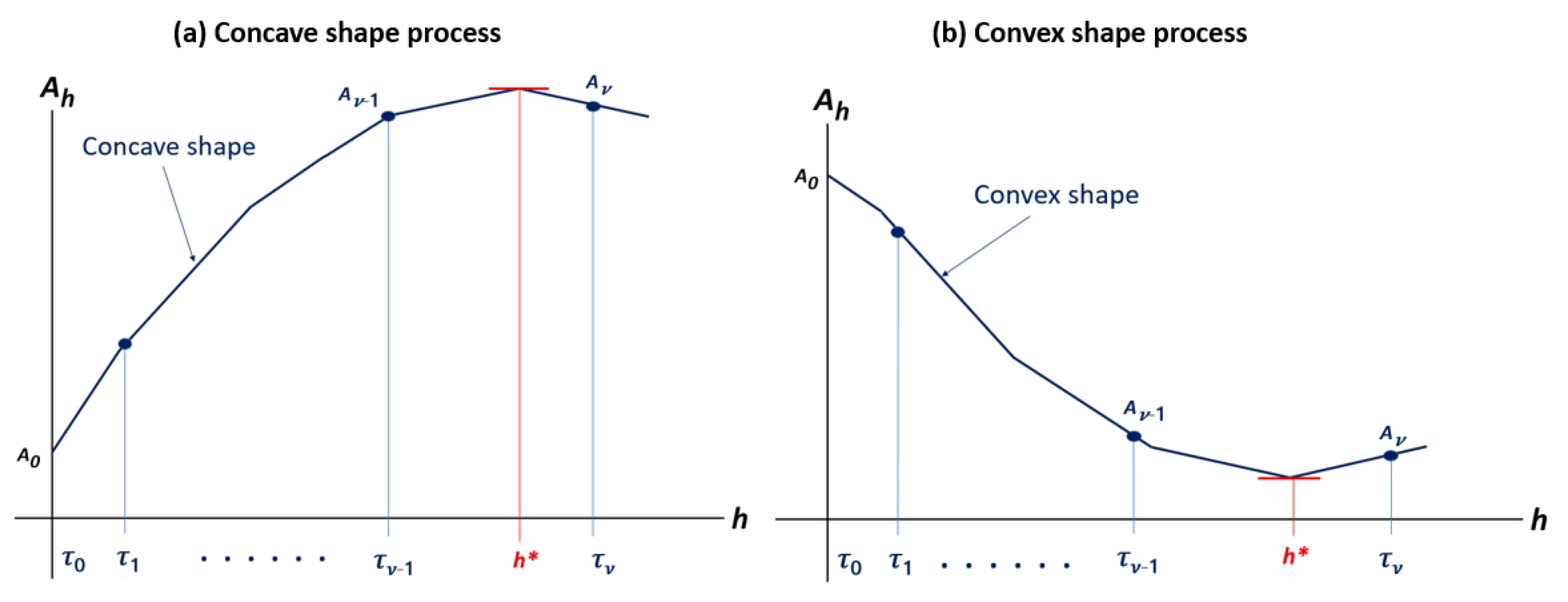
Figure 2.
SBFP on NASDAQ 100 stock chart for 6 months (Source: etoro.com).

Figure 3.
Find the optimal moment using Matlab.


Table 1.
Cost matrix.
| Up | Down | |
|---|---|---|
| Hold | ||
| Action |
Publisher’s Note: MDPI stays neutral with regard to jurisdictional claims in published maps and institutional affiliations. |
© 2022 by the author. Licensee MDPI, Basel, Switzerland. This article is an open access article distributed under the terms and conditions of the Creative Commons Attribution (CC BY) license (https://creativecommons.org/licenses/by/4.0/).
Share and Cite
MDPI and ACS Style
Kim, S.-K. Shifted Brownian Fluctuation Game. Mathematics 2022, 10, 1735. https://doi.org/10.3390/math10101735
AMA Style
Kim S-K. Shifted Brownian Fluctuation Game. Mathematics. 2022; 10(10):1735. https://doi.org/10.3390/math10101735
Chicago/Turabian StyleKim, Song-Kyoo (Amang). 2022. "Shifted Brownian Fluctuation Game" Mathematics 10, no. 10: 1735. https://doi.org/10.3390/math10101735
APA StyleKim, S.-K. (2022). Shifted Brownian Fluctuation Game. Mathematics, 10(10), 1735. https://doi.org/10.3390/math10101735
Note that from the first issue of 2016, this journal uses article numbers instead of page numbers. See further details here.