Study of Solutions for a Degenerate Reaction Equation with a High Order Operator and Advection

Abstract

The goal of the present study is to characterize solutions under a travelling wave formulation to a degenerate Fisher-KPP problem. With the degenerate problem, we refer to the following: a heterogeneous diffusion that is formulated with a high order operator; a non-linear advection and non-Lipstchitz spatially heterogeneous reaction. The paper examines the existence of solutions, uniqueness and travelling wave oscillatory properties (also called instabilities). Such oscillatory behaviour may lead to negative solutions in the proximity of zero. A numerical exploration is provided with the following main finding to declare: the solutions keeps oscillating in the proximity of the null stationary solution due to the high order operator, except if the reaction term is quasi-Lipschitz, in which it is possible to define a region where solutions are positive locally in time.

1. Introduction and Problem Outline

The seminal work proposed by the scientists Kolmogorov, Petrovskii and Piskunov [1] (to study combustion phenomena) and by Fisher [2] (to understand the interactions of genes) introduced a novel methodology on how to search for solutions in non-linear reaction-diffusion problems. The proposed solutions were known as travelling waves and the main idea was to find a travelling speed for which the associated solution was monotone and stable, i.e., the solution did not oscillate. Afterwards, the proposed methodology was widely considered for modelling in different sciences: from biology and ecology (refer to [3,4,5]) to fluid dynamics [6].

The problem introduced in this study can be considered as highly degenerate. Indeed, this is because of the heterogeneous diffusion, the non-linear reaction term and the non-linearity in the advection term.

Firstly, the diffusion is given by a high order spatial operator. This kind of operator allows us to account for an heterogeneous diffusion in a given domain (see [7]). High order operators have attracted interest to model unstable patterns of heteroclinic solutions in bi-stable systems ([8,9,10,11]). In addition, the Giorgi’s conjecture to an Allen-Cahn equation formulated with a high order operator has been provided in [12].

Other types of heterogeneous diffusion for Fisher-KPP problems have been contemplated, for instance, the p-Laplacian operator in [13], the p-Laplacian with non-Lipschitz reaction in [14] and the doubly nonlinear diffusion in [15,16]. Considering the advection term, well-posedness and regularity of solutions have been provided by Montaru in [17].

The proposed analysis in this paper considers the travelling waves formulation that has provided important achievements to model in different scenarios (refer to [18] for wide discussion together with [19,20,21]) including heterogeneous diffusion (see [22,23,24,25]) and porous medium degenerate diffusion [26,27,28].

Heterogeneity in the Fisher-KPP reaction term is a research topic of interest. Indeed, in [29], the authors provide existence analysis in the travelling wave domain to an heterogeneous (in space and time) Fisher-KPP equation. Additional analysis in relation with high order operators can be found in [30,31,32].

The proposed problem (P), set in Equation (1), is constituted of three degenerate terms: a heterogeneous diffusion formulated with a order four operator, a non-linear advection term and a non-Lipschitz reaction. In addition, assume that the initial condition belongs to the bounded space of locally square integrable functions.

$$\begin{array}{c}{w}_t=-{\Delta }^{2}w+c{\left(w^q\right)}_x+{|x|}^{\delta }{w}^p(a-w),\\ w_0\left(x\right)\in L_{loc}^2\left(R\right)\cap L^{\infty }\left(R\right),\\ w_{0,x}\in L^q\left(R\right),\\ 0<p<1,q>1,\delta >0,a>1.\end{array}$$

(1)

The main novelty introduced is related with the treatment of the three discussed degenerate terms and the theoretical aspects to study existence and uniqueness of positive solutions. In case positivity does not hold, the intention is to search for specific conditions in the involved parameters $p,q,\delta$ for which solutions may be positive globally or in a certain region locally in time.

Firstly, regularity results are obtained based on the formulation of the problem as an abstract evolution of a super continuous semi-group for which a fix point argument is employed (see [33] for a fixed point theorem formulation applicable to analysis of existence topics). Afterwards, the instabilities of travelling profiles are characterized. This is an important aspect as it permits to confirm that the high degenerate problem provides inherently unstable patterns of solutions. As discussed, the presence of a non-linear advection and a degenerate reaction shall be investigated. Particularly, to determine if under certain conditions positivity of solutions may hold in the proximity of zero. Such searching of positivity (and smoothness) is explored based on numerical evidences. To make the numerical exploration tractable, the bvp4c function in MATLAB is used to provide graphical representation of solutions. It shall be noted that such representation provided aims at introducing the equation dynamics. A similar approach in this regards can be consulted in [34], where a graphical design introduces the dynamics of a space-time fractional nonlinear Bogoyavlenskii equation and a Schrödinger equation. As our intention is to characterize positivity of solutions, the analysis is performed in one dimension, $x\in R$. Nonetheless, in case of higher spatial dimensions, the MATLAB function bvp4c may not be valid. In this case, solutions shall be found based in mesh-less methods for solving transport phenomena (the reader is referred to [35] as a representative example of this approach).

2. Assessment on Regularity, Existence and Uniqueness

2.1. Previous Definitions and Supporting Results

Definition 1.

Assume the following definition of a norm in a Hilbert–Sobolev space $H_{\alpha }^4\left(R\right)$:

$${\parallel w\parallel }_{\alpha }^2={\int }_R\alpha \left(\zeta \right)\sum _{k=0}^4{|D^{k}w\left(\zeta \right)|}^{2}d\zeta ,$$

(2)

such that $D=\frac{d}{d\zeta }$, and the function $w\in (H_{\alpha }^4\cap W^{4,2})\left(R\right)\subset L_{\alpha }^2\left(R\right)\subset L^2\left(R\right)$. The weight $\alpha \left(\zeta \right)$ is given by (see [17,23]):

$$\alpha \left(\zeta \right)=e^{a_0{|\zeta |}^{\frac{4}{3}}-a_1{|\zeta |}^{\delta }-\frac{1}{{\zeta }^q}\frac{1}{t^{\gamma }}{\int }_0^t({\parallel w_x\left(\tau \right)\parallel }^q+1)d\tau },$$

(3)

where $a_0>0$ is a sufficiently small constant and $0<a_1<<1$ is determined locally for $|w(x,t_0)|<<1$ (to have the exponential behaviour $e^{-a_1{|\zeta |}^{\delta }}$) and $\gamma >q+1$.

As the intention is to study oscillating (in the sense of unstable) solutions, a mollifying norm in a Sobolev space is introduced. The mollifying kernel is of the exponential type.

Definition 2.

For $j\in R^{+}$ and $0\le t<\infty$, the following norm is defined in a weighted Sobolev space $H^j$:

$${\parallel w\parallel }_{H^j}^2={\int }_{-\infty }^{\infty }{e}^{j{\omega }^2}{|\widehat{w}(\omega ,t)|}^{2}d\omega ,$$

(4)

where the exponential kernel complies with the $A_p$-condition for $(p=1)$ [36].

The coming proposition is well-known from the theory of Sobolev spaces and continuity embedding. To this end, assume a sequence of open bounded intervals $U_n\subset R$ such that $U_n=\{x\in B(0,n),n\in N\}$:

Proposition 1.

Consider the Sobolev space $W^{m,p}\left(U_n\right)$ and define $k=int\{m-\frac{1}{p}\}$, then the following continuous (in the sense of Hölder) inclusion holds (see [37], p. 79):

$$W^{m,p}\left(U_n\right)\hookrightarrow C^k\left(U_n\right).$$

(5)

Note that in our case $m=4$, $p=2$ then $k=3$.

2.2. Solution Bounds and Regularity

Consider the general homogeneous problem:

$$w_t=Lw,$$

(6)

where $L=(-D_x^4+q{w}^{q-1}c{D}_x)$ is a formal representation.

The following bounds hold:

Lemma 1.

Consider the square integral function $w_0\in L^2\left(R\right)$:

$${\parallel w\parallel }_{L^2}\le {\parallel w_0\parallel }_{L^2}.$$

(7)

In addition, assume $w_0\in H^j\left(R\right)\cap L^2\left(R\right)$, then:

$${\parallel w\parallel }_{H^j}\le {\parallel w_0\parallel }_{H^j},{\parallel w\parallel }_{H^j}\le {\parallel w_0\parallel }_{L^2},fort\ge \frac{j}{4}.$$

(8)

Finally:

$${\parallel w\parallel }_{\alpha }\le {\rm Y}{\parallel w\parallel }_{H^j}\le {\rm Y}{\parallel w_0\parallel }_{H^j},{{\rm Y}}^2=25max\{w,D^{1}w,D^{2}w,D^{3}w,D^{4}w\},$$

(9)

where the order four derivative shall comply with the sub-exponential behaviour:

$$|D^{4}w\left(\zeta \right)|<e^{-{|\zeta |}^{\frac{4}{3}}},$$

(10)

whenever $|w|\to 0$.

Proof. 

Given the single Equation (6), the following abstract representation holds:

$$w(x,t)=e^{tL}{w}_0\left(x\right),$$

(11)

and making the Fourier transformation (f-domain):

$$\widehat{w}(f,t)=e^{t(-f^4+2\pi fci\widehat{w^q})}{\widehat{w}}_0\left(f\right).$$

(12)

Considering the Fourier isometric condition under $L^2$ norm:

$$\begin{array}{cc}\hfill {\parallel w\parallel }_{L^2}^2& ={\int }_{-\infty }^{\infty }|e^{2t(-f^4+2\pi fci\widehat{w^q})}{|}^2|{\widehat{w}}_0\left(f\right){|}^{2}df={\int }_{-\infty }^{\infty }{e}^{-2f^{4}t}{|{\widehat{w}}_0\left(f\right)|}^{2}df\hfill \\ & \le \underset{f\in R}{sup}\left(e^{-2f^{4}t}\right){\int }_{-\infty }^{\infty }{|{\widehat{w}}_0\left(f\right)|}^{2}df={\parallel w_0\parallel }_{L^2}^2.\hfill \end{array}$$

(13)

Concluding on ${\parallel w\parallel }_{L^2}\le {\parallel w_0\parallel }_{L^2}$.

Now, consider the weighted Sobolev space $H^j$ with norm (4). The following bound holds:

$$\begin{array}{cc}\hfill {\parallel w\parallel }_{H^j}^2& ={\int }_{-\infty }^{\infty }{e}^{j{f}^2}|\widehat{w}(f,t){|}^{2}df={\int }_{-\infty }^{\infty }{e}^{j{f}^2}|e^{2t(-f^4+2\pi fci\widehat{w^q})}||{\widehat{w}}_0\left(f\right){|}^{2}df\hfill \\ & \le \underset{f\in R}{sup}\left(e^{-2f^{4}t}\right){\int }_{-\infty }^{\infty }{e}^{j{f}^2}{|{\widehat{w}}_0\left(f\right)|}^{2}df={\parallel w_0\parallel }_{H^j}^2.\hfill \end{array}$$

(14)

Initially, it has been requested $w_0\in L^2\left(R\right)$, then:

$${\parallel w\parallel }_{H^j}^2={\int }_{-\infty }^{\infty }{e}^{j{f}^2}|\widehat{w}(f,t){|}^{2}df\le \underset{f\in R}{sup}\left(e^{j{f}^2}{e}^{-2f^{4}t}\right){\int }_{-\infty }^{\infty }{|{\widehat{w}}_0\left(f\right)|}^{2}df.$$

(15)

After standard assessments:

$${\parallel w\parallel }_{H^j}^2\le {\left(\frac{j}{4t}\right)}^{1/2}{\parallel w_0\parallel }_{L^2}^2.$$

(16)

Concluding on:

$${\parallel w\parallel }_{H^j}\le {\parallel w_0\parallel }_{L^2},$$

(17)

for $t\ge \frac{j}{4}$.

Considering the weighted Sobolev space $H_{\alpha }^4$ with norm (2):

$$\begin{array}{cc}\hfill {\parallel w\parallel }_{\alpha }^2& ={\int }_R\alpha \left(\zeta \right)\sum _{k=0}^4|D^{k}w\left(\zeta \right){|}^{2}d\zeta \le {\int }_R{e}^{j{\zeta }^2}\sum _{k=0}^4{|D^{k}w\left(\zeta \right)|}^{2}d\zeta \hfill \\ & \le {{\rm Y}}^2{\int }_{U_{n\to \infty }}{e}^{j{\zeta }^2}{|w\left(\zeta \right)|}^{2}d\zeta \le {{\rm Y}}^2{\parallel w\parallel }_{H^j}^2.\hfill \end{array}$$

(18)

For the last inequality, the continuity Proposition 1 has been considered, so that, the following scaling variable is defined upon: ${{\rm Y}}^2=25{sup}_{\zeta \in U_{n\to \infty }}\{w,D^{1}w,D^{2}w,D^{3}w,D^{4}w\}$. Note that the Proposition 1 permits to account for the regularity in the involved derivatives. The fourth derivative in ${\rm Y}$ can be considered as a controlling parameter. Indeed, the inequality (18) states that any function, under norm $H_{\alpha }^4$, can be bounded by the mollifying norm (4) provided there exists a finite value of ${\rm Y}$. In case any of the derivatives (but certainly the fourth) in ${\rm Y}$ is not controlled, because of the presence of high instabilities in the solutions, then the inequality (18) states that the norm $H_{\alpha }^4$ is not mollified, leading to high values in ${\rm Y}$ that predominate over the mollifying norm. In this case, it shall be required ${\parallel w\parallel }_{H^j}\to 0$ to balance cases of $|{\rm Y}|>>1$ because of a potentially uncontrolled order four derivative. In our case, it is the idea to study solutions in the proximity of the null state, $w=0$; therefore, it is natural to assume ${\parallel w\parallel }_{H^j}\to 0$. Furthermore, and according to [23], the global decreasing behaviour of solutions is below an exponential behaviour. Then, it is required that a four order derivative shall comply:

$$|D^{4}w\left(\zeta \right)|<e^{-{|\zeta |}^{\frac{4}{3}}}.$$

(19)

We have shown that the mollifying space $H^j$ is bounded by the norm $L^2$ defined for square integrable initial data. Furthermore, the weighted space $H_{\alpha }^4$ has been proved to be bounded by the space $H^j$ of mollified solutions, multiplied by the scaling term ${\rm Y}$. □

The fourth order operator, $-{\Delta }^2$, can be regarded as the infinitesimal representation of a singe parametric (with $0<\tau \le t$) strongly continuous semi-group. Hence, an abstract form to represent the evolving solution is given by:

$$w\left(\tau \right)=e^{-{\Delta }^2\tau }{w}_0+{\int }_0^{\tau }\left[c·\nabla e^{-{\Delta }^2(\tau -s)}{w}^q\left(s\right)+e^{-{\Delta }^2(\tau -s)}{|x|}^{\delta }{w}^p\left(s\right)(a-w\left(s\right))\right]ds.$$

(20)

A solution to the homogeneous problem $w_t=-{\Delta }^{2}w,$ with pulse shape initial data $w(x,0)=\delta \left(x\right)$ is:

$$\widehat{w}\left(t\right)=e^{-f^{4}t}{\widehat{w}}_0.$$

(21)

A kernel to the homogeneous equation is given by:

$$N(x,t)=F^{-1}\left(e^{-f^{4}t}\right)=\frac{1}{2\pi }{\int }_R{e}^{-f^{4}t-ifx}df={\int }_R{e}^{-f^{4}t}cos\left(fx\right)df.$$

(22)

The integral (22) convergences for $f\in R$. Consequently, a kernel $N(x,t)$ does exist.

Consider the following operator defined as a mapping:

$${\Sigma }_{w_0,t}:H_{\alpha }^4\left(R\right)\to H_{\alpha }^4\left(R\right),$$

(23)

for $0<\tau \le t$, such that:

$$\begin{array}{cc}\hfill {\Sigma }_{w_0,t}\left(v\right)& =N(x,t)\ast w_0\left(x\right)+{\int }_0^{\tau }[c·\nabla N(x,t-s)\ast w^q(x,s)\hfill \\ & +N(x,t-s)\ast \{|x{|}^{\delta }{w}^p(x,s)(a-w(x,s))\}]ds.\hfill \end{array}$$

(24)

The following Lemma holds:

Lemma 2.

The operator ${\Sigma }_{w_0,t}$ (where t refers to a free parameter) is bounded in the space $H_{\alpha }^4\left(R\right)$ under norm (2).

Proof. 

As a previous step, the inequality $B_0{\parallel w_0\parallel }_{\alpha }\le {\parallel w\parallel }_{\alpha }$ (being $B_0>0$ a suitable constant) is proved:

$$\begin{array}{cc}\hfill {\parallel w\parallel }_{\alpha }^2& ={\int }_R\alpha \left(\zeta \right)\sum _{k=0}^4|D^k\widehat{w}\left(\zeta \right){|}^{2}d\zeta ={\int }_R\alpha \left(\zeta \right)\sum _{k=0}^4{|D^k\left[e^{t(-{\zeta }^4+2\pi \zeta ci\widehat{w^q})}{\widehat{w}}_0\right]|}^{2}d\zeta \hfill \\ & \ge {\int }_R\alpha \left(\zeta \right)\sum _{k=0}^4|D^k\left[e^{t(-{\zeta }^4+2\pi \zeta ci\widehat{w^q})}\right]{|}^2\sum _{k=0}^4{|D^k{\widehat{w}}_0|}^{2}d\zeta \hfill \\ & \ge B_0^2{\int }_R\alpha \left(\zeta \right)\sum _{k=0}^4{|D^k{\widehat{w}}_0|}^{2}d\zeta =B_0^2{\parallel w_0\parallel }_{\alpha }^2,\hfill \end{array}$$

(25)

where $B_0^2={inf}_{\zeta \in B_r}\{{\sum }_{k=0}^4|D^k\left[e^{t(-{\zeta }^4+2\pi \zeta ci\widehat{w^q})}\right]{|}^2\}>0$ is required to be small in $B_r=\{\zeta ,|\zeta |<r\}$ for $r>0$.

Now, considering the single parametric operator ${\Sigma }_{w_0,t}$:

$$\begin{array}{cc}\hfill & {\parallel {\Sigma }_{w_0,t}\left(w\right)\parallel }_{\alpha }={\parallel {\Sigma }_{w_0,t}\parallel }_{\alpha }{\parallel w\parallel }_{\alpha }\le {\parallel N\parallel }_{\alpha }{\parallel w_0\parallel }_{\alpha }+{\int }_0^{\tau }[{\parallel c·\nabla N\parallel }_{\alpha }{\parallel w^q\parallel }_{\alpha }\hfill \\ & +{\parallel N\parallel }_{\alpha }{\parallel |x|}^{\delta }{\parallel }_{\alpha }{\parallel w\parallel }_{\alpha }^p{\parallel a-w\parallel }_{\alpha }]ds\hfill \\ & \le \left[{\parallel N\parallel }_{\alpha }\frac{1}{B_{0}t}+{\int }_0^{\tau }\left[{\parallel c·\nabla N\parallel }_{\alpha }{\parallel w_0^{q-1}\parallel }_{H^j}+{\parallel N\parallel }_{\alpha }{\parallel |x|}^{\delta }{\parallel }_{\alpha }{\parallel w\parallel }_{\alpha }^{p-1}|{\parallel a\parallel }_{\alpha }-B_0{\parallel w_0\parallel }_{\alpha }|\right]ds\right]\hfill \\ & t{\parallel w\parallel }_{\alpha }.\hfill \end{array}$$

(26)

Consider the inequalities in (14) and (18) to the terms ${\parallel w^{q-1}\parallel }_{\alpha }$ and ${\parallel w^{p-1}\parallel }_{\alpha }$:

$${\parallel w^{q-1}\parallel }_{\alpha }\le {\parallel w^{q-1}\parallel }_{H^j}\le {\parallel w_0^{q-1}\parallel }_{H^j},{\parallel w^{p-1}\parallel }_{\alpha }\le {\parallel w^{p-1}\parallel }_{H^j}\le {\parallel w_0^{p-1}\parallel }_{H^j}.$$

(27)

Based on these inequalities and the convergent kernel $N(x,t)$ shown in (22) (${\parallel N\parallel }_{\alpha }$ finite), we conclude that the right hand side term in (26) is indeed bounded. Therefore, the mapping ${\Sigma }_{w_0,t}$, $\forall t>0$ is bounded. □

2.3. Uniqueness

The objective in this section is to show that the mapping ${\Sigma }_{w_0,t}$ as defined in (23) has a single fix point, i.e., $w(x,t)={\Sigma }_{w_0,t}\left(w(x,t)\right)$. To this end, the following holds:

$$\begin{array}{cc}\hfill & {\parallel {\Sigma }_{w_0,t}\left(w_1\right)-{\Sigma }_{w_0,t}\left(w_2\right)\parallel }_{\alpha }\le {\int }_0^{\tau }\parallel c·\nabla N(x,t-s)\ast (w_1^q-w_2^q)+\hfill \\ & N(x,t-s)\ast [w_1^p(a-w_1)-w_2^p(a-w_2)]{\parallel |x|}^{\delta }{{\parallel }_{\alpha }\parallel }_{\alpha }ds\hfill \\ & ={\int }_0^{\tau }\parallel {\int }_{\tau }^s\{c·\nabla N(x,t-s-\nu )(w_1^q-w_2^q)\hfill \\ & +N(x,t-s-\nu )[w_1^p(a-w_1)-w_2^p(a-w_2)]{\parallel |x|}^{\delta }{\parallel }_{\alpha }{\}d\nu \parallel }_{\alpha }ds\hfill \\ & \le {\int }_0^{\tau }{\int }_{\tau }^s\{{\parallel c·\nabla N(x,t-s-\nu )(w_1^q-w_2^q)\parallel }_{\alpha }\hfill \\ & +{\parallel N(x,t-s-\nu )[w_1^p(a-w_1)-w_2^p(a-w_2)]\parallel }_{\alpha }{\parallel |x|}^{\delta }{\parallel }_{\alpha }\}d\nu ds\hfill \\ \hfill & ={\int }_0^{\tau }{\int }_{\tau }^s{\{\parallel c·\nabla N(x,t-s-\nu )\parallel }_{\alpha }{\parallel w_1^q-w_2^q\parallel }_{\alpha }\hfill \\ & +{\parallel N(x,t-s-\nu )\parallel }_{\alpha }{\parallel w_1^p(a-w_1)-w_2^p(a-w_2)\parallel }_{\alpha }{\parallel |x|}^{\delta }{\parallel }_{\alpha }\}d\nu ds\hfill \\ \hfill & \le \Lambda {\int }_0^{\tau }{\int }_{\tau }^s\{{\parallel w_1^q-w_2^q\parallel }_{\alpha }+{\parallel w_1^p(a-w_1)-w_2^p(a-w_2)\parallel }_{\alpha }{\parallel |x|}^{\delta }{\parallel }_{\alpha }\}d\nu ds.\hfill \end{array}$$

(28)

Note that N and $\nabla N$ are bounded functions as per the converge condition in (22), then:

$$\Lambda =sup\{{\parallel N(x,t-s-\nu )\parallel }_{\alpha },{\parallel c·\nabla N(x,t-s-\nu )\parallel }_{\alpha };x\in R,\forall t>0,\}$$

(29)

is finite $\forall s$ and $\forall \nu$.

The intention now is to assess each of the integrals in (28). To this end, the following supporting functions are previously defined:

$$A(ϵ,s)=\left\{\begin{array}{c}\frac{w_1{(ϵ,s)}^q-w_2{(ϵ,s)}^q}{w_1(ϵ,s)-w_2(ϵ,s)}for{w}_1\not\equiv w_2\\ q{w}_1^{q-1}otherwise\end{array}\right\},B(ϵ,s)=\left\{\begin{array}{c}\frac{w_1{(ϵ,s)}^p-w_2{(ϵ,s)}^p}{w_1(ϵ,s)-w_2(ϵ,s)}for{w}_1\not\equiv w_2\\ p{w}_1^{p-1}otherwise\end{array}\right\}.$$

(30)

Given fixed values for $ϵ$ and s, the functions $A(ϵ,s)$ and $B(ϵ,s)$ are bounded. Hence, assume the following definitions of $c_0$ and $k_0$:

$$0\le A(ϵ,s)\le c_0(q,\parallel w_0{\parallel }_{\infty },T),0\le B(ϵ,s)\le k_0(p,\parallel w_0{\parallel }_{\infty },T).$$

(31)

So that:

$$|w_1^q-w_2^q|\le c_0|w_1-w_2|,|w_1^p-w_2^p|\le k_0|w_1-w_2|.$$

(32)

In the proximity of the stationary solution $w=a$, any solution is convergent (this is further analyzed in the travelling waves study afterwards). Hence, consider $M=max\{a-w_1,a-w_2\}$:

$$\begin{array}{cc}\hfill & {\parallel [w_1^p(a-w_1)-w_2^p(a-w_2)]\parallel }_{\alpha }^2={\int }_R\alpha \left(\zeta \right)\sum _{k=0}^4{|D^k[w_1^p(a-w_1)-w_2^p(a-w_2)]|}^{2}d\zeta \hfill \\ \hfill & ={\int }_R\alpha \left(\zeta \right)\left\{|w_1^p(a-w_1)-w_2^p(a-w_2){|}^2+\sum _{k=1}^4{|D^k[w_1^p(a-w_1)-w_2^p(a-w_2)]|}^2\right\}d\zeta \hfill \\ \hfill & \le 25M{\int }_R\alpha \left(\zeta \right)\left\{k_0^2|(w_1-w_2){|}^2+\sum _{k=1}^4\sum _{i=1}^k{k}_0^2{|D^k|w_1-w_2||}^2\right\}d\zeta \hfill \\ \hfill & =25M{k}_0^2{\int }_R\alpha \left(\zeta \right)\sum _{k=0}^4{|D^k[w_1-w_2]|}^{2}d\zeta =25M{k}_0^2{\parallel w_1-w_2\parallel }_{\alpha }^2.\hfill \end{array}$$

(33)

Consequently:

$$\begin{array}{cc}\hfill {\parallel {\Sigma }_{w_0,t}\left(w_1\right)-{\Sigma }_{w_0,t}\left(w_2\right)\parallel }_{\alpha }& \le M^{1/2}(5k_0{\parallel |x|}^{\delta }{\parallel }_{\alpha }+c_0){\int }_0^{\tau }{\int }_{\tau }^s{\parallel w_1-w_2\parallel }_{\alpha }dsd\nu \hfill \\ & =M^{1/2}(5k_0{\parallel |x|}^{\delta }{\parallel }_{\alpha }+c_0)\tau (\tau -s){\parallel w_1-w_2\parallel }_{\alpha },\hfill \end{array}$$

(34)

where the term ${\parallel |x|}^{\delta }{\parallel }_{\alpha }<\infty$ under the norm in (2).

Given a ball centered in $0<\tau \le t$ with an amplitude as a multiple of $\tau -s$, uniqueness applies in the limit $w_1\swarrow w_2$ resulting in a contractive ${\Sigma }_{w_0,t}$, such that ${\Sigma }_{w_0,t}\left(w_1\right)\swarrow w_1$ in the space $H_{\alpha }^4$.

3. Travelling Waves

Travelling waves profiles are given by $w(x,t)=\chi \left(\omega \right),\omega =x·n_d-\lambda t\in R$, being $n_d\in R$ a unit vector providing the travelling wave propagation direction, $\lambda$ is the travelling wave velocity and $\chi \in L_{loc}^2\left(R\right)\cap L^{\infty }\left(R\right)$ or $\chi \in L^2\left(R\right)\cap L^{\infty }\left(R\right)\cap H_{\alpha }^4\left(R\right)$, $\xi \in L^2\left(R\right)\cap L^{\infty }\left(R\right)\cap H^4\left(R\right)$ in the proximity of the stationary solutions $w=0$ and $w=a$.

For $n_d=(1,0,...,0)$, $w(x,t)=\chi \left(\omega \right),\omega =x-\lambda t\in R$.

In the sake of simplicity, the advection vector c acts in the same direction $n_d$. Hence:

$$-\lambda {\chi }^{\prime }=-{\chi }^{\left(4\right)}+c{\left({\chi }^q\right)}_x+{|x|}^{\delta }{\chi }^p(a-\chi ).$$

(35)

Consider a truncation for the term ${|x|}^{\delta }$, to control the growing behaviour of the degenerate reaction:

$${|x|}_{ϵ}^{\delta }=\left[\begin{array}{c}{|x|}^{\delta },0\le |x|<ϵ\\ {ϵ}^{\delta },|x|\ge ϵ\end{array}\right].$$

(36)

Then, the associated problem $P^{\prime }$ is given as:

$$-\lambda {\chi }^{\prime }=-{\chi }^{\left(4\right)}+c{\left({\chi }^q\right)}_x+{|x|}_{ϵ}^{\delta }{\chi }^p(a-\chi )\le -{\chi }^{\left(4\right)}+c{\left({\chi }^q\right)}_x+{ϵ}^{\delta }{\chi }^p(a-\chi ).$$

(37)

Note that the truncated term ${|x|}_{ϵ}^{\delta }$ allows us to define finite balls in the spatial domain where the travelling wave profiles evolve. Based on this, the following Lemma characterizes the travelling waves motion:

Lemma 3.

The travelling wave velocity λ is positive (i.e., the travelling waves moves from $\omega \to -\infty$ to $\omega \to \infty$) provided the following condition is met:

$$c>\frac{\left(\frac{1}{p+1}a-\frac{1}{p+2}\right){ϵ}^{\delta }}{q\left(\frac{1}{q-1}-2\right)},$$

(38)

where ${ϵ}^{\delta }>0$. The travelling wave velocity λ is negative for $c<\frac{\left(\frac{1}{p+1}a-\frac{1}{p+2}\right){ϵ}^{\delta }}{q\left(\frac{1}{q-1}-2\right)}$. Furthermore, the travelling wave stops for $c=\frac{\left(\frac{1}{p+1}a-\frac{1}{p+2}\right){ϵ}^{\delta }}{q\left(\frac{1}{q-1}-2\right)}.$

Proof. 

Multiply (37) by ${\chi }^{\prime }$:

$$-\lambda {\left({\chi }^{\prime }\right)}^2=-{\chi }^{\left(4\right)}{\chi }^{\prime }+c{\left({\chi }^q\right)}_x{\chi }^{\prime }+{ϵ}^{\delta }a{\chi }^p{\chi }^{\prime }-{ϵ}^{\delta }{\chi }^{p+1}{\chi }^{\prime },$$

(39)

Upon integration in each of the terms:

$$\begin{array}{cc}\hfill \int {\chi }^{\left(4\right)}{\chi }^{\prime }& ={\chi }^{\prime }{\chi }^{\left(3\right)}-\int {\chi }^{\left(3\right)}{\chi }^{\left(2\right)}={\chi }^{\prime }{\chi }^{\left(3\right)}-\left({\chi }^{\left(2\right)}{\chi }^{\left(2\right)}-\int {\chi }^{\left(2\right)}{\chi }^{\left(3\right)}\right)\hfill \\ \hfill & ={\chi }^{\prime }{\chi }^{\left(3\right)}-{\chi }^{\left(2\right)}{\chi }^{\left(2\right)}+\int {\chi }^{\left(2\right)}{\chi }^{\left(3\right)}={\chi }^{\prime }{\chi }^{\left(3\right)}-{\chi }^{\left(2\right)2}+{\chi }^{\prime }{\chi }^{\left(3\right)}-\int {\chi }^{\left(4\right)}{\chi }^{\prime }.\hfill \end{array}$$

(40)

Then

$$\int {\chi }^{\left(4\right)}{\chi }^{\prime }=\frac{1}{2}(2{\chi }^{\prime }{\chi }^{\left(3\right)}-{\chi }^{\left(2\right)2}).$$

(41)

The last integral is calculated between $\omega \to -\infty$ and $\omega \to +\infty$. In addition and in the asymptotic approximation, we consider:

$$\begin{array}{c}{\chi }^{\prime }(-\infty )={\chi }^{\left(2\right)}(-\infty )={\chi }^{\left(3\right)}(-\infty )=0,\\ \\ {\chi }^{\prime }(\infty )={\chi }^{\left(2\right)}(\infty )={\chi }^{\left(3\right)}(\infty )=0.\end{array}$$

(42)

As a consequence:

$${\int }_{-\infty }^{\infty }{\chi }^{\left(4\right)}{\chi }^{\prime }=0.$$

(43)

Now, for the integral involving the advection term:

$$c\int {\left({\chi }^q\right)}_x{\chi }^{\prime }=c{\left({\chi }^q\right)}_x\chi -c\int q(q-1){\chi }^{q-1}{\chi }^{\prime }-cq\int {\chi }^q{\chi }^{\left(2\right)}.$$

(44)

Note that $\int {\chi }^{q-1}{\chi }^{\prime }={\chi }^{q-1}\chi -\int {\left({\chi }^{q-1}\right)}_x\chi ,$$\int {\chi }^q{\chi }^{\left(2\right)}={\chi }^q{\chi }^{\prime }-\int {\left({\chi }^q\right)}_x{\chi }^{\prime }$.

Compiling all the exposed:

$$(1-q)c\int {\left({\chi }^q\right)}_x{\chi }^{\prime }=-cq(q-1){\chi }^q+cq(q-1)\int \chi {\left({\chi }^{q-1}\right)}_x.$$

(45)

Again, the integral on the right reads:

$$\int \chi {\left({\chi }^{q-1}\right)}_x=\frac{1}{q-1}{\chi }^q-{\chi }^q,$$

(46)

so that:

$$c{\int }_{-\infty }^{\infty }{\left({\chi }^q\right)}_x{\chi }^{\prime }=cq{\left(2{\chi }^q-\frac{1}{q-1}{\chi }^q\right)}_{-\infty }^{\infty }=cq\left(\frac{1}{q-1}-2\right).$$

(47)

Now, the integrals involving the reaction terms read:

$$\int {\chi }^p{\chi }^{\prime }={\chi }^p\chi -\int p{\chi }^p{\chi }^{\prime }\to {\int }_{-\infty }^{\infty }{\chi }^p{\chi }^{\prime }=\frac{1}{p+1}{\left[{\chi }^p\chi \right]}_{-\infty }^{\infty }=\frac{1}{p+1}(0-1)=-\frac{1}{p+1}.$$

(48)

Similarly:

$$\int {\chi }^{p+1}{\chi }^{\prime }=-\frac{1}{p+2}.$$

(49)

Compiling, in (39), the different integrals assessed:

$$-\lambda \int {\left({\chi }^{\prime }\right)}^2=0+cq\left(\frac{1}{q-1}-2\right)-\frac{1}{p+1}a{ϵ}^{\delta }+\frac{1}{p+2}{ϵ}^{\delta },$$

(50)

such that

$$\lambda =\frac{\left(2-\frac{1}{q-1}\right)cq+\frac{1}{p+1}a{ϵ}^{\delta }-\frac{1}{p+2}{ϵ}^{\delta }}{\int {\left({\chi }^{\prime }\right)}^2}.$$

(51)

Note that $ϵ>0$. In addition, $a>1$, then the term:

$$\frac{1}{p+1}a{ϵ}^{\delta }-\frac{1}{p+2}{ϵ}^{\delta }>0.$$

The problem P is recovered for $ϵ\to \infty$, then the expression obtained for $\lambda$ permits to prove the lemma postulations. □

3.1. Instabilities in the Domain of Travelling Waves

The objective in this section is to characterize instability of travelling wave profiles close the critical points in (37) at $\chi =0$ and $\chi =a$. The analysis followed is based on a set of Theorems and Lemmas that were previously introduced to study unstable spatial patterns of solutions in a high order operator with odd spatial derivative [25], in a Cahn–Hilliard equation [24] and in a Kuramoto–Sivashinsky equation [38]. Note that some modifications are encountered in our analysis compared to that in the previous equations mentioned.

Lemma 4.

Consider the Hilbert–Sobolev spaces $H^4$, $H_{\alpha }^4$. In addition, consider the Lebesgue $L^2$. The following inequalities hold: ${\parallel w\parallel }_{L^2}\le C_1{\parallel w\parallel }_{H^4}$, ${\parallel w\parallel }_{L^2}\le C_2{\parallel w\parallel }_{\alpha }$ i.e., any finite mass solution is bounded by the space of oscillating solutions.

Proof. 

Based on (4):

$${\parallel w\parallel }_{H^4}={\int }_R{e}^{4{\omega }^2}|\widehat{w}(\omega ,t){|}^{2}d\omega \ge \underset{\omega \in (-\infty ,\infty )}{inf}\{e^{4{\omega }^2}\}{\int }_R{|\widehat{w}(\omega ,t)|}^{2}d\omega ={\parallel w\parallel }_{L^2},$$

(52)

which implies $C_1=1$. Now, considering the norm in (2):

$${\parallel w\parallel }_{L^2}\le {\int }_R\sum _{k=0}^4|D^{k}w\left(\zeta \right){|}^{2}d\zeta \le {\int }_R\alpha \left(\zeta \right)\sum _{k=0}^4{|D^{k}w\left(\zeta \right)|}^{2}d\zeta ={\parallel w\parallel }_{\alpha },$$

(53)

a.e. in R. Then it suffices to assume $C_2=1$ □

Convergence of travelling waves profiles to the stationary solutions $w=0$ and $w=a$ can be studied based on the definition of a perturbed function, $\mu (x,t)$, that measures the distance between the actual solution and the travelling wave profile: $\mu (x,t)=w(x,t)-\chi (x,t)$. The problem P (1) is now formulated with the new function $\mu$ and the profile $\chi$ in the proximity of $\mu =0$ and considering $w(x,t)=\mu (x,t)+\chi (x,t)$. Note that the main terms are given by the high order operator as a source of unstable patterns and the advection term that introduces derivatives as well:

$${\mu }_t=-{\mu }^{\left(4\right)}+\frac{1}{2}\sum _{k=0}^{\infty }\left(\genfrac{}{}{0pt}{}{q}{k}\right)(q-k)c{\mu }^{q-k-1}{\chi }^q{\mu }_x+\frac{c}{2}\sum _{k=0}^{\infty }\left(\genfrac{}{}{0pt}{}{q}{k}\right){\mu }^{q-k}{\chi }^{q-1}{\chi }_x.$$

(54)

Assume the definition of:

$${\mu }_t=L_0\mu +\Phi \left(\mu \right),$$

(55)

where $L_0=-D_x^4$ and $\Phi \left(\mu \right)=\frac{1}{2}{\sum }_{k=0}^{\infty }\left(\genfrac{}{}{0pt}{}{q}{k}\right)(q-k)c{\mu }^{q-k-1}{\chi }^q{\mu }_x+\frac{c}{2}{\sum }_{k=0}^{\infty }\left(\genfrac{}{}{0pt}{}{q}{k}\right){\mu }^{q-k}{\chi }^{q-1}{\chi }_x$.

The coming Lemma aims to provide bounds to the advection term:

Lemma 5. 

$\Phi :H^4\to L^2$ is a continuous mapping. In addition, there exist ${\epsilon }_0>0$, $\epsilon >1$ and $C_3>0$ such that ${\parallel \Phi \left(\mu \right)\parallel }_{L^2}<C_3{\parallel \mu \parallel }_{H^4}^{\epsilon }$, provided $0<{\parallel \mu \parallel }_{H^4}<{\epsilon }_0$.

Proof. 

$$\begin{array}{cc}\hfill {\parallel \Phi \left(\mu \right)\parallel }_{L^2}& \le {\parallel \Phi \left(\mu \right)\parallel }_{H^4}\le \frac{1}{2}\sum _{k=0}^{\infty }\left(\genfrac{}{}{0pt}{}{q}{k}\right)(q-k)c{\parallel {\mu }^{q-k-1}\parallel }_{H^4}{\parallel {\chi }^q\parallel }_{\infty }{\omega }_1{\parallel \mu \parallel }_{H^4}\hfill \\ & +\frac{c}{2}\sum _{k=0}^{\infty }\left(\genfrac{}{}{0pt}{}{q}{k}\right){\parallel {\mu }^{q-k-1}\parallel }_{H^4}\parallel \mu \parallel {\parallel {\chi }^{q-1}\parallel }_{\infty }{\parallel {\chi }_x\parallel }_{\infty },\hfill \end{array}$$

(56)

where the constant ${\omega }_1>0$ comes from the local application of Gronwall‘s inequality ${\parallel {\mu }_x\parallel }_{H^4}\le {\omega }_1{\parallel \mu \parallel }_{H^4}$. Then:

$${\parallel \Phi \left(\mu \right)\parallel }_{H^4}\le ({\parallel {\chi }^q\parallel }_{\infty }{\omega }_1+{\parallel {\chi }^{q-1}\parallel }_{\infty }{\parallel {\chi }_x\parallel }_{\infty })\frac{c}{2}\sum _{k=0}^{\infty }\left(\genfrac{}{}{0pt}{}{q}{k}\right)(q-k){\parallel \mu \parallel }_{H^4}^{-k-1}{\parallel \mu \parallel }_{H^4}^{q+1}.$$

(57)

$${\parallel \Phi \left(\mu \right)\parallel }_{L^2}\le {\parallel \Phi \left(\mu \right)\parallel }_{H^4}\le C_3{\parallel \mu \parallel }_{H^4}^{\epsilon },$$

(58)

such that $\epsilon =q+1$ and $C_3=({\parallel {\chi }^q\parallel }_{\infty }{\omega }_1+{\parallel {\chi }^{q-1}\parallel }_{\infty }{\parallel {\chi }_x\parallel }_{\infty })\frac{c}{2}{\sum }_{k=0}^{\infty }\left(\genfrac{}{}{0pt}{}{q}{k}\right)(q-k)N$, for a sufficiently large $N\ge {\sum }_{k=0}^{\infty }{\parallel \mu \parallel }_{H^4}^{-k-1}$. □

It shall be noted that the last Lemma can be similarly treated for the mapping $\Phi :H_{\alpha }\to L^2$, provided there exist $r>0$, $\epsilon >1$ and $C_4>0$ such that ${\parallel \Phi \left(\mu \right)\parallel }_{L^2}<C_4{\parallel \mu \parallel }_{\alpha }^{\epsilon }$, for $0<{\parallel \mu \parallel }_{\epsilon }<r$. In this case $C_4=({\parallel {\chi }^q\parallel }_{\infty }{\omega }_1+{\parallel {\chi }^{q-1}\parallel }_{\infty }{\parallel {\chi }_x\parallel }_{\infty })\frac{c}{2}{\sum }_{k=0}^{\infty }\left(\genfrac{}{}{0pt}{}{q}{k}\right)(q-k)N_1$, for a sufficiently big $N_1\ge {\sum }_{k=0}^{\infty }{\parallel \mu \parallel }_{\alpha }^{-k-1}$.

The mapping ${\Sigma }_{{\mu }_0,t}$ is bounded (refer to Lemma 2), then and considering the exponential representation to the linear operator $L_0$, the following Lemma is shown:

Lemma 6.

The high order linear operator $L_0$ generates the bounded abstract evolution $e^{t{L}_0}$ that complies with:

$${\int }_0^1{\parallel e^{t{L}_0}\parallel }_{L^2\to H^4}=A_1<\infty ,{\int }_0^1{\parallel e^{t{L}_0}\parallel }_{L^2\to H_{\alpha }^4}=A_2<\infty$$

(59)

Proof. 

First, the following exponential representation holds for any homogeneous solution:

$$\widehat{\mu }(f,t)=e^{-t{f}^4}{\widehat{\mu }}_0\left(f\right).$$

(60)

Then

$${\parallel \mu \parallel }_{H^4}\le {\parallel e^{-t{f}^4}\parallel }_{H^4}{\parallel {\mu }_0\parallel }_{H^4}\le \underset{f\in (-\infty ,\infty )}{sup}\{e^{4f^2-2t{f}^4}\}{\parallel {\mu }_0\parallel }_{L^2},$$

(61)

$${\parallel e^{-t{f}^4}\parallel }_{L^2\to H^4}{\parallel {\mu }_0\parallel }_{L^2}\le {\parallel e^{-t{f}^4}\parallel }_{H^4}{\parallel {\mu }_0\parallel }_{H^4}\le \underset{f\in (-\infty ,\infty )}{sup}\{e^{4f^2-2t{f}^4}\}{\parallel {\mu }_0\parallel }_{L^2}.$$

(62)

Then

$${\parallel e^{-t{f}^4}\parallel }_{L^2\to H^4}\le \underset{f\in (-\infty ,\infty )}{sup}\{e^{4f^2-2t{f}^4}\}=e^{2t^{-1}},0<t\le 1.$$

(63)

A finite $A_1$ is get after integration with regards to t in the interval $(0,1]$. Similarly, for $A_2$:

$$\begin{array}{cc}\hfill {\parallel \mu \parallel }_{\alpha }^2& ={\int }_R\alpha \left(f\right)\sum _{k=0}^4|D^k\widehat{\mu }\left(f\right){|}^{2}df\le 2{{\rm Y}}^2{\int }_{R^{+}}{e}^{a_0{f}^{4/3}}{|\widehat{\mu }\left(f\right)|}^{2}df\hfill \\ & \le 2{{\rm Y}}^2{\int }_{R^{+}}{e}^{a_0{f}^{4/3}-2t{f}^4}{|{\widehat{\mu }}_0\left(f\right)|}^{2}df\le 2{{\rm Y}}^2\underset{f\in (0,\infty )}{sup}\{e^{a_0{f}^{4/3}-2t{f}^4}\}{\parallel {\mu }_0\parallel }_{L^2}^2\hfill \\ & =2{{\rm Y}}^2{e}^{A_c{a}_0^{3/2}{t}^{-1/2}}{\parallel {\mu }_0\parallel }_{L^2}^2,{\parallel \mu \parallel }_{\alpha }\le 2^{\frac{1}{2}}{\rm Y}{e}^{\frac{A_c}{2}{a}_0^{3/2}{t}^{-1/2}}{\parallel {\mu }_0\parallel }_{L^2}.\hfill \end{array}$$

(64)

where $A_c>0$ is a suitable constant obtained after standard operations. Note that ${\parallel e^{-t{f}^4}\parallel }_{L^2\to H_{\alpha }^4}{\parallel {\mu }_0\parallel }_{L^2}\le {\parallel \mu \parallel }_{\alpha }$, and

$${\parallel e^{-t{f}^4}\parallel }_{L^2\to H_{\alpha }^4}\le 2^{\frac{1}{2}}{\rm Y}{e}^{\frac{A_c}{2}{a}_0^{3/2}{t}^{-1/2}}.$$

(65)

A finite value for $A_2$ is obtained upon integration with regards to t in the interval $(0,1]$. □

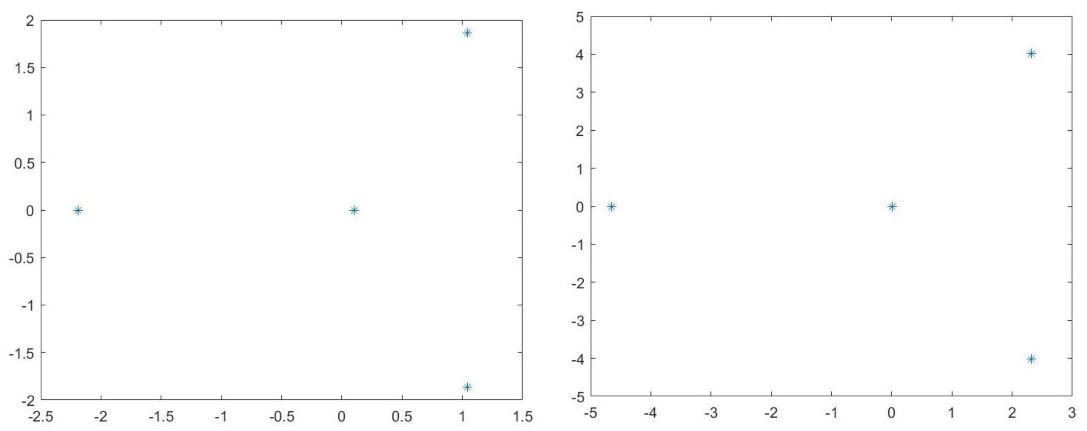
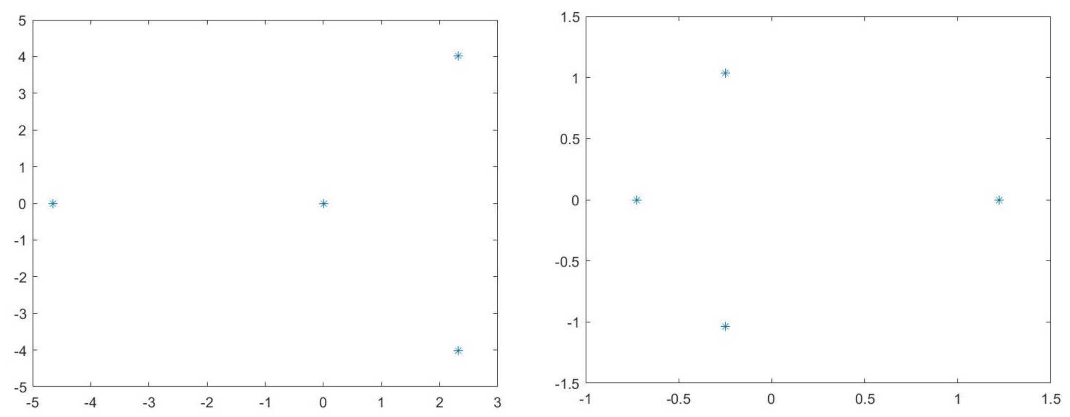
The following objective consists on characterizing the spectrum of the operator L in the proximity of the critical points. To this end, it shall be considered that the inherent instability criteria requires L to satisfy the following Lemma:

Lemma 7.

The local spectrum of L (6) in $H^4$, in the proximity of the equilibrium at $w=0$ and $w=a$, has at least one eigenvalue (s) with positive real part ($Re\left(s\right)>0)$.

Proof. 

The local spectrum of L can be shown based on the theory of Evans functions (refer to [39]). In our case, we make use of a symbolic matrix representation to a linearized approach close the equilibrium points $w=0$ and $w=a$. To understand the influence of the travelling wave velocity, $\lambda$, a parametric analysis is presented in the form of homotopy graphs. First of all, assume the symbolic representation of (35) given by:

$${\left(\begin{array}{c}{\chi }_1\\ {\chi }_2\\ {\chi }_3\\ {\chi }_4\end{array}\right)}^{\prime }=\left(\begin{array}{cccc}0& 1& 0& 0\\ 0& 0& 1& 0\\ 0& 0& 0& 1\\ (a-{\chi }_1){|x|}_{ϵ}^{\delta }& \lambda +cq{\chi }_1^{q-1}& 0& 0\end{array}\right)\left(\begin{array}{c}{\chi }_1\\ {\chi }_2\\ {\chi }_3\\ {\chi }_4\end{array}\right)$$

(66)

$${\chi }^{\prime }=E(c,a,\lambda ,x)F.$$

(67)

Such that the characteristic polynomial to the matrix E is given by:

$$P\left(s\right)=s^4-(cq{\chi }_1^{q-1}+\lambda )s+({\chi }_1-a){|x|}_{ϵ}^{\delta }=0.$$

(68)

assume the approximation ${\chi }_1<ϵ\to 0$, then it is easily checked that $P\left(s\right)$ has at least one root with positive real part. Given an arbitrary $ϵ$ in ${|x|}_{ϵ}^{\delta }$ and for $0<s<<1$ we have $P\left(s\right)<0$, now for $s>>1$, $P\left(s\right)>0$. To further understand the root behaviours to the polynomial $P\left(s\right)$ and with no loss of generality, assume ${|x|}_{ϵ}^{\delta }=1$ (see Figure 1, Figure 2, Figure 3 and Figure 4 to check on the root behaviour for different travelling waves velocities).

In the proximity of the equilibrium state ${\chi }_1=a$ and considering ${|x|}_{ϵ}^{\delta }=1$, the homotopy graphs show that there exists one eigengavalue s with positive real part (refer to Figure 5 and Figure 6). Alternatively, this can be easily assessed to be $s={\left(cq{a}^{q-1}+\lambda \right)}^{\frac{1}{3}}$. □

3.2. Travelling Wave Exact Profiles and Positivity Conditions

As discussed in Lemma 7, there exist complex roots associated to oscillating flows of solutions. Consequently, the philosophy initially provided in the seminal work in [1] cannot be systematically followed. Indeed, the oscillating profiles induced by the high order operator make impossible to find a critical travelling wave speed for which oscillations do not exist, leading to purely monotonic exponential solutions. As an alternative idea, the problem is translated into searching for an appropriate travelling wave velocity for which solutions are positive in the first minimum and locally in time. The localization of such minimum is carried out in the travelling wave solutions and, likely, only in a local close domain in virtue of the heterogeneity in the reaction term. Hence, and in general, we postulate that it is not possible to search for global positive solutions $\forall \omega \in R$, due to the introduced degenerate reaction and to the inherent instabilities associated to the operator (shown in Section 3.1 that impedes the formulation of a maximum principle).

The analysis of exact travelling waves profiles is performed with the function bvp4c in MATLAB. This function employs an implicit Runge-Kutta with interpolant extensions [40]. Furthermore, the solver is based on a collocation procedure for which pseudo-boundary conditions shall be specified. In our case, the initial condition is given as a Heaviside step function of the form $w_0\left(x\right)=aH(-x)$. This function is relevant as it allows us to understand the behaviour of a positive initial mass (at $x=\omega <0$) and a null mass (for $x=\omega >0$). In addition, an heteroclinic connection is given between the two stationary solutions at $w_0(x<0)=a$ and $w_0(x>0)=0$. To avoid the impact of the pseudo-boundary conditions, required by the collocation method, the domain has been considered large enough, i.e. $\omega \in (-1000,1000)$. In addition, the maximum error assumed is ${10}^{-5}$ and the number of nodes in the domain has been defined accordingly to 100,000.

Our idea is to explore the existence of a specific value in the variable $\Pi =\lambda t$ for which the first travelling profile minimum is positive. The numerical routine has been executed for $\lambda =1$ with no loss of generality, so that a wide interval of t values have been introduced until the first profile minimum is positive. The numerical analysis reveals that it is not possible to find a unique travelling wave speed (valid for any time) for which the first minimum is positive, and hence, providing a stationary inner region of positive solutions. This observation is caused by the heterogeneous reaction. On the contrary, we show that the non-Lipschitz reaction term keeps solutions unstable. Further, the analysis is explored for p values close to one, where it is possible to conclude that positivity holds for a certain travelling wave speed and locally in time. In addition, it shall be assumed that the travelling profile moves from left to right, i.e. for particular values in p, a, $\delta$ and q, the advection coefficient c shall comply with (38). To make the problem tractable, assume that $q=2$, $p=0.5$ (afterwards $p=0.999$ to explore quasi-Lipschitz conditions), $a=1$ and $c=1$.

Based on the discussions hold, the following Lemma aims to compile the main findings.

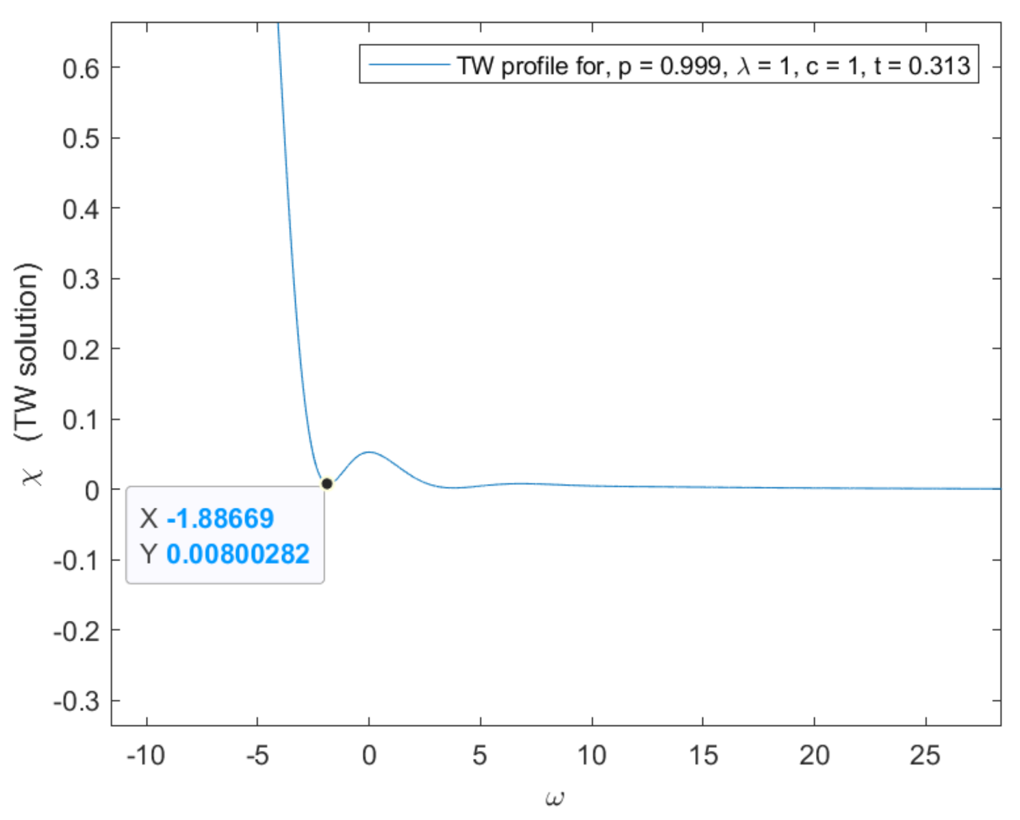
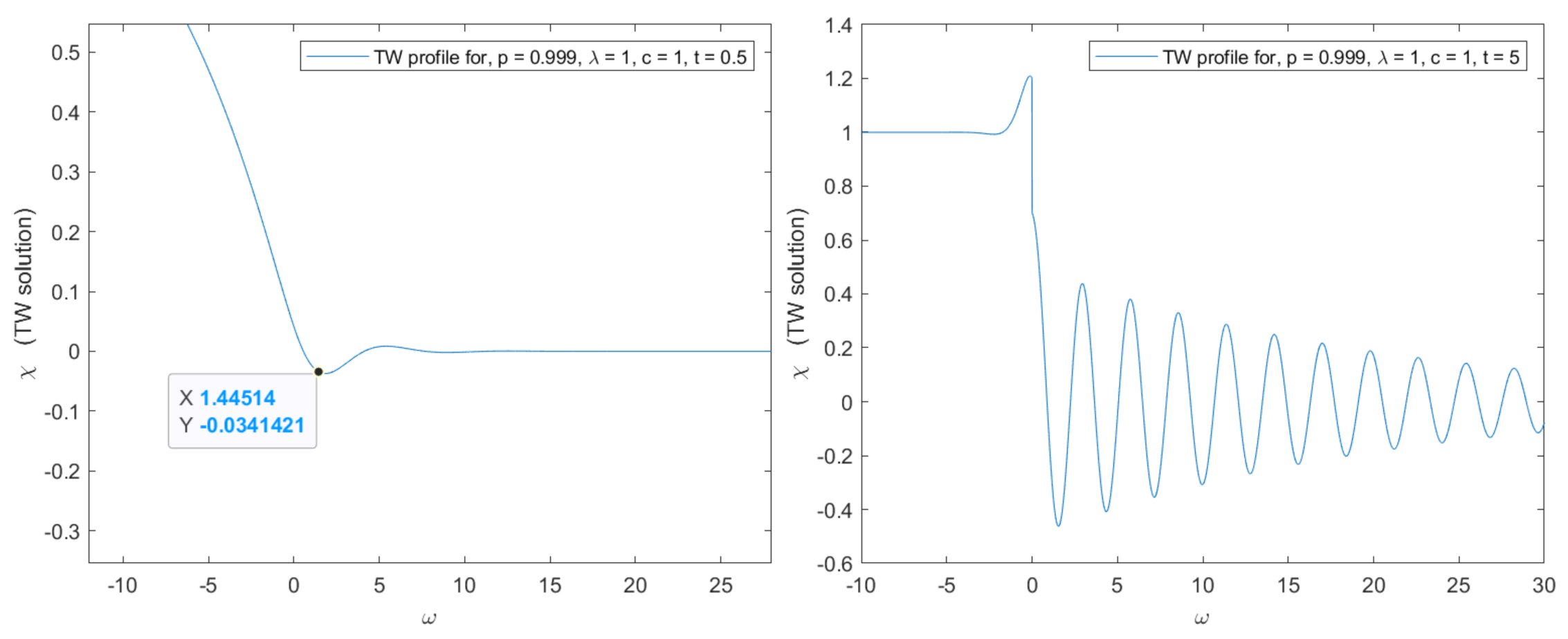
Lemma 8.

Consider the set $M_{\Pi }$::

$$M_{\Pi }=min\{\Pi =\lambda t/\chi >0,{\chi }^{\prime }=0,{\chi }^{″}>0\},$$

(69)

which provides a set whose elements permit to localize the minimum values of $\chi \left(\omega \right)$ in the travelling wave tail.

For $p$-values in the range $0<p<1$ (i.e., non-Lipschitz reaction) solutions are oscillating for any time. For $p$-values close to one (quasi-Lipschitz conditions), it is possible to conclude on the existence of a first positive minimum such that $\chi \left(M_{\Pi }\right)>0$.

Proof. 

The proof of the proposed Lemma is based on the numerical findings compiled in Figure 7, Figure 8, Figure 9, Figure 10 and Figure 11. Note that the determination of a general $\Pi$ is difficult in a general sound given the number of involved parameters. To avoid this issue, the numerical explorations have been pursuit for the different values provided in the Figures. Note that when $p\to 1$, the reaction term becomes slightly Lipschitz, then it is possible to conclude on the existence of a local positive first minimum (see Figure 10). Considering the travelling waves variable $\omega =x-\Pi$ and given the results in Figure 10, it is possible to determine an $x$-region of positivity, indeed:

$$|x|=1.567.$$

(70)

Note that this region of positive solutions only holds for quasi-Lipschitz reaction and locally for $t=0.313$. For $t>0.313$, positivity in the quasi-Lipschitz case does not hold in general (refer to Figure 11). □

4. Conclusions

The analysis provided has shown the bound properties of solutions in generalized Hilbert–Sobolev spaces together with existence and uniqueness results upon the definition of an abstract evolution. Afterwards, solutions have been shown to exhibit oscillatory patterns due to the fourth order operator. The oscillating behavior of solutions was explored based on a set of Lemmas (from Lemma 4 to 7) already used to study a high order operator with odd spatial derivative [25], a Cahn–Hilliard equation [24] and a Kuramoto–Sivashinsky equation [38]. Eventually, a numerical routine is provided in the search of travelling waves profiles together with regions where conditions to characterize positive solutions hold. As a main finding, it was observed that solutions are oscillating in the proximity of the null critical point (and hence being negative since the first minimum) due to the non-Lipschitz reaction term. On the contrary, when the reaction term is quasi-Lipschitz ($p=0.999$), it is possible to define a region where solutions are positive locally in time. The numerical exploration was executed for specific values in the parameters p, c, q and a, but conclusions remain valid for any other combination. i.e., a region of positive solutions holds only in the quasi-Lipschitz case.

References

1. Kolmogorov, A.N.; Petrovskii, I.G.; Piskunov, N.S. Study of the diffusion equation with growth of the quantity of matter and its application to a biological problem. Byull. Moskov. Gos. Univ. 1937, 1, 1–25. [Google Scholar]
2. Fisher, R.A. The advance of advantageous genes. Ann. Eugen. 1937, 7, 355–369. [Google Scholar] [CrossRef] [Green Version]
3. Aronson, D. Density-dependent interaction-diffusion systems. In Proc. Adv. Seminar on Dynamics and Modeling of Reactive System; Academic Press: New York, NY, USA, 1980. [Google Scholar]
4. Aronson, D.; Weinberger, H. Nonlinear diffusion in population genetics, combustion and nerve propagation. In Partial Differential Equations and Related Topic; Springer: New York, NY, USA, 1975; pp. 5–49. [Google Scholar]
5. Aronson, D.; Weinberger, H. Multidimensional nonlinear diffusion arising in population genetics. Adv. Math. 1978, 30, 33–76. [Google Scholar] [CrossRef] [Green Version]
6. Ladyzhenskaya, O. Some results on modifications of three-dimensional Navier-Stokes equations. In Nonlinear Analysis and Continuum Mechanics; Springer: New York, NY, USA, 1998; pp. 73–84. [Google Scholar]
7. Cohen, D.S.; Murray, J.D. A generalized diffusion model for growth and dispersal in a population. J. Math. Biol. 1981, 12, 237–249. [Google Scholar] [CrossRef]
8. Audrito, A. Bistable and monostable reaction equations with doubly nonlinear diffusion. Discrete Contin. Dyn. Syst. 2019, 39, 2977–3015. [Google Scholar] [CrossRef] [Green Version]
9. Bonheure, D.; Sánchez, L. Heteroclinics Orbits for Some Classes of Second and Fourth Order Differential Equations. In Handbook of Differential Equations; Elsevier: Amsterdam, The Netherlands, 2006; Volume 3, pp. 103–202. [Google Scholar]
10. Dee, G.T.; Van Sarloos, W. Bistable systems with propagating fronts leading to pattern formation. Phys. Rev. Lett. 1998, 60. [Google Scholar] [CrossRef] [Green Version]
11. Peletier, L.A.; Troy, W.C. Spatial Patterns. Higher order models in Physics and Mechanics. In Progress in Non Linear Differential Equations and Their Applications; Université Pierre et Marie Curie: Paris, France, 2001; Volume 45. [Google Scholar]
12. Bonheure, D.; Hamel, F. One-dimensional symmetry and Liouville type results for the fourth order Allen-Cahn equation in R. Chin. Ann. Math. Ser. B 2017, 38, 149–172. [Google Scholar] [CrossRef] [Green Version]
13. Audrito, A.; Vázquez, J.L. The Fisher–KPP problem with doubly nonlinear “fast” diffusion. Nonlinear Anal. 2017, 157, 212–248. [Google Scholar] [CrossRef] [Green Version]
14. Díaz, J.L. Non-Lipschitz heterogeneous reaction with a p-Laplacian operator. AIMS Math. 2022, 7, 3395–3417. [Google Scholar] [CrossRef]
15. Audrito, A.; Vázquez, J.L. The Fisher-KPP problem with doubly nonlinear diffusion. J. Differ. Equ. 2017, 263, 7647–7708. [Google Scholar] [CrossRef] [Green Version]
16. Du, Y.; Gárriz, A.; Quirós, F. Travelling-wave behaviour in doubly nonlinear reaction-diffusion equations. arXiv 2009, arXiv:2009.12959. [Google Scholar]
17. Montaru, A. Wellposedness and regularity for a degenerate parabolic equation arising in a model of chemotaxis with nonlinear sensitivity. Discret. Contin. Dyn. Syst. 2014, 231–256. [Google Scholar] [CrossRef]
18. Gilding, B.H.; Kersner, R. Travelling waves in nonlinear diffusion-convection reaction. In Progress in Nonlinear Differential Equations and Their Applications; Springer: Basel, Switzerland, 2004. [Google Scholar]
19. Durham, A.C.; Ridgway, E.B. Control of chemotaxis in physarum polycephalum. J. Cell. Biol. 1976, 69, 218–223. [Google Scholar] [CrossRef] [PubMed] [Green Version]
20. Niemela, J.J.; Ahlers, G.; Cannell, D.S. Localized traveling-wave states in binary-fluid convection. Phys. Rev. Lett. 1990, 64, 1365–1368. [Google Scholar] [CrossRef] [PubMed]
21. Rauprich, O.; Matsushita, M.; Weijer, C.J.; Siegert, F.; Esipov, S.E.; Shapiro, J.A. Periodic phenomena in proteus mirabilis swarm colony development. J. Bacteriol. 1996, 178, 6525–6538. [Google Scholar] [CrossRef] [Green Version]
22. Galaktionov, V.A. On a spectrum of blow-up patterns for a higher-order semilinear parabolic equation. Proc. R. Soc. A Math. Phys. Eng. Sci. 2001. [Google Scholar] [CrossRef]
23. Galaktionov, V. Towards the KPP–Problem and Log-Front Shift for Higher-Order Nonlinear PDEs I. Bi-Harmonic and Other Parabolic Equations. arXiv 2012, arXiv:1210.3513. [Google Scholar]
24. Gao, H.; Liu, C. Instabilities of traveling waves of the convective-diffusive Cahn–Hilliard equation. Chaos Solitons Fractals 2004, 20, 253–258. [Google Scholar]
25. Li, Z.; Liu, C. On the Nonlinear Instability of Traveling waves for a Sixth-Order Parabolic Equation. Abstr. Appl. Anal. 2012, 17, 739156. [Google Scholar] [CrossRef]
26. De Pablo, A.; Vázquez, J.L. Travelling Waves and Finite Propagation in a Reaction-Diffusion Equation. J. Differ. Equ. 1991, 93, 19–61. [Google Scholar] [CrossRef] [Green Version]
27. Du, Y.; Quirós, F.; Zhou, M. Logarithmic corrections in Fisher-KPP type Porous Medium Equations. J. Math. Pures Appl. 2020, 136, 415–455. [Google Scholar] [CrossRef] [Green Version]
28. Gárriz, A. Propagation of solutions of the Porous Medium Equation with reaction and their travelling wave behaviour. Nonlinear Anal. 2020, 195, 1–23. [Google Scholar] [CrossRef] [Green Version]
29. Nadin, G.; Rossi, L. Transition waves for Fisher-KPP equations with general time-heterogeneous and space-periodic coefficients. Analysis 2015, 8, 1351–1377. [Google Scholar] [CrossRef]
30. Akveld, M.E.; Hulshof, J. travelling wave Solutions of a Fourth-Order Semilinear Diffusion Equation. Appl. Math. Lett. 1998, 11, 115–120. [Google Scholar] [CrossRef] [Green Version]
31. Egorov, Y.; Galaktionov, V.; Kondratiev, V.; Pohozaev, S. Global solutions of higher-order semilinear parabolic equations in the supercritical range. Adv. Differ. Equat. 2004, 9, 1009–1038. [Google Scholar] [CrossRef]
32. Rottschäfer, V.; Doelman, A. On the transition from the Ginzburg-Landau equation to the extended Fisher-Kolmogorov equation. Physica D 1998, 118, 261–292. [Google Scholar] [CrossRef] [Green Version]
33. Benchohra, M.; Medjadj, I. Measure of Noncompactness and Partial Functional Differential Equations with State-Dependent Delay. Differ. Equ. Dyn. Syst. 2018, 26, 139–155. [Google Scholar] [CrossRef]
34. Alam, N.; Tunç, C. The new solitary wave structures for the (2 + 1)-dimensional time-fractional Schrodinger equation and the space-time nonlinear conformable fractional Bogoyavlenskii equations. Alex. Eng. J. 2020, 59, 2221–2232. [Google Scholar] [CrossRef]
35. Lin, J.; Bai, J.; Reutskiy, S.; Lu, J. A novel RBF-based meshless method for solving time-fractional transport equations in 2D and 3D arbitrary domains. Eng. Comput. 2022, 1–18. [Google Scholar] [CrossRef]
36. Goldshtein, V.; Ukhlov, A. Weighted Sobolev Spaces and embeddings Theorems. Trans. Am. Math. Soc. 2009, 361, 3829–3850. [Google Scholar] [CrossRef] [Green Version]
37. Kesavan, S. Topics in Functional Analysis and Applications; New Age International (formerly Wiley-Eastern): Hoboken, NJ, USA, 1989. [Google Scholar]
38. Strauss, W.; Wang, G. Instabilities of travelling waves of the Kuramoto–Sivashinsky equation. Chin. Ann. Math. B 2002, 23, 267–276. [Google Scholar] [CrossRef]
39. Alexander, J.; Gardner, R.; Jones, C. A topological invariant arising in the stability analysis of travelling waves. J. Reine Angew. Math. 2020, 410, 167–212. [Google Scholar] [CrossRef]
40. Enright, H.; Muir, P.H. A Runge-Kutta Type Boundary Value ODE soLwer with Defect Control; Teh. Rep. 267/93; University of Toronto, Department of Computer Sciences: Toronto, ON, Canada, 1993. [Google Scholar]
Figure 1. λ = 1 (left) and λ = 10 (right). P ( s ) roots evolution in the complex domain (Real part in the horizontal and Imaginary in the vertical) for a = 1 , with χ 1 < ϵ 0 and | x | ϵ δ = 1 . It shall be noted that there exists at least one root R e ( s ) > 0 .
Mathematics 10 01729 g001
Figure 2. Root evolution for λ = 100 (left) and λ = 1000 (right). To this end, a = 1 , with χ 1 < ϵ 0 and | x | ϵ δ = 1 . It shall be noted that there exists at least one root R e ( s ) > 0 .
Mathematics 10 01729 g002
Figure 3. Root evolution for λ = 1 (left) and λ = 10 (right). To this end, a = 1 , with χ 1 < ϵ 0 and | x | ϵ δ = 1 . It shall be noted that there exists at least one root R e ( s ) > 0 .
Mathematics 10 01729 g003
Figure 4. Idem for λ = 100 (left) and λ = 1000 (right). To this end, a = 1 , with χ 1 < ϵ 0 and | x | ϵ δ = 1 . It shall be noted that there exists at least one root R e ( s ) > 0 .
Mathematics 10 01729 g004
Figure 5. λ = 1 (left) and λ = 1000 (right). P ( s ) roots evolution in the complex domain (Real part in the horizontal and Imaginary in the vertical) for a = 1 , with χ 1 a and | x | ϵ δ = 1 . It shall be noted that there exists at least one root R e ( s ) > 0 .
Mathematics 10 01729 g005
Figure 6. Idem for λ = 1 (left) and λ = 1000 (right). To this end, a = 1 , with χ 1 a and | x | ϵ δ = 1 . It shall be noted that there exists at least one root R e ( s ) > 0 .
Mathematics 10 01729 g006
Figure 7. Travelling wave profile evolution for p = 0.5 . It is possible to observe that the first minimum is negative for each given time.
Mathematics 10 01729 g007
Figure 8. Idem for higher time values.
Mathematics 10 01729 g008
Figure 9. Similarly for other time values with p = 0 , 5 .
Mathematics 10 01729 g009
Figure 10. Positivity in the first minimum holds for p close to one (i.e., close to a Lipschitz reaction term). In this case Π = λ t = 0.313 . For Π < 0.313 , solution profiles have a negative first minimum. Idem for Π > 0.313 , refer to Figure 11.
Mathematics 10 01729 g010
Figure 11. For a quasi-Lipschitz reaction, solutions keep oscillating for t > 0.313 .
Mathematics 10 01729 g011
Publisher’s Note: MDPI stays neutral with regard to jurisdictional claims in published maps and institutional affiliations.