A Hybridized Mixed Approach for Efficient Stress Prediction in a Layerwise Plate Model

Abstract

Building upon recent works devoted to the development of a stress-based layerwise model for multilayered plates, we explore an alternative finite-element discretization to the conventional displacement-based finite-element method. We rely on a mixed finite-element approach where both stresses and displacements are interpolated. Since conforming stress-based finite-elements ensuring traction continuity are difficult to construct, we consider a hybridization strategy in which traction continuity is relaxed by the introduction of an additional displacement-like Lagrange multiplier defined on the element facets. Such a strategy offers the advantage of uncoupling many degrees of freedom so that static condensation can be performed at the element level, yielding a much smaller final system to solve. Illustrative applications demonstrate that the proposed mixed approach is free from any shear-locking in the thin plate limit and is more accurate than a displacement approach for the same number of degrees of freedom. As a result, this method can be used to capture efficiently strong intra- and inter-laminar stress variations near free-edges or cracks.

1. Introduction

Multilayered plates are important in structural engineering and are widely studied by engineers during the 20th century with applications ranging from aerospace engineering to civil engineering. The materials in each layer can be either homogeneous and isotropic or heterogeneous and anisotropic (e.g., fiber-reinforced composites). The difficulty in studying such structures comes from the strong variations of mechanical properties between each ply, especially when using anisotropic materials. Free-edge effects have been a source of many difficulties, both in terms of design or analysis of multilayered plates. In fact, near free edges, there are highly concentrated interlaminar stresses [1,2,3,4,5]. Such stress concentrations are important to account for since they are at the origin of interlayer delamination and failure of the laminate. Many models have been proposed to correctly account for such detrimental effects. If three-dimensional (3D) finite-element methods allow for an accurate modeling of stress singularities near regions of interest, they require well-refined meshes and therefore cannot model a whole laminated plate without tremendous numerical cost. Moreover, traditional finite-element approaches are based on displacement interpolation which make the corresponding stress predictions less accurate than stress-based methods. On the contrary, two-dimensional plate models aim at providing a much simpler representation of the mechanical fields through the thickness and are therefore less computationally demanding. The main challenge is related to the efficiency of the underlying through-the-thickness hypothesis which should result in a sufficiently accurate representation of local 3D displacement and stress fields.

A first approach concerns equivalent single layer (ESL) models which replace the laminate as an equivalent homogeneous plate. Most of them are based on higher order theories [6,7,8,9,10,11,12,13,14,15]. If the prediction of the global structural response of the laminate is generally good, the investigation of the local 3D fields near regions of strong singularities is in general not satisfying.

Instead of replacing the laminate with a single plate, layerwise models consider instead the laminate as a collection of layers with their own plate-like kinematics in order to improve the accuracy of the 3D local fields representation [16,17,18,19,20,21]. Obviously more expensive than the ESL model, they are an interesting alternative to fully 3D models since they rely on physically-motivated through-the-thickness assumptions. A general review of the development of layerwise models can be found in [22,23,24].

Many layerwise models are based on a kinematic assumptions of the 3D displacement fields. However, it is known that such a hypothesis will not necessarily satisfy interlayer traction continuity for instance. Conversely, a collection of stress-based layerwise models has been proposed in [25,26,27,28,29,30,31,32,33,34] following the ideas first proposed in [35]. In the so-called LS1 model, the laminate can be seen as a collection of Reissner–Mindlin plates which are connected with each other through interlaminar stresses which are part of the model generalized stresses. The construction of the LS1 model is however not completely based on stress-like assumptions as some equilibrium conditions are not enforced exactly. To circumvent this drawback, a fully statically compatible LS1 (SCLS1) model has been developed more recently [36]. The SCLS1 model is fully statically compatible in the sense that it produces a 3D stress field which satisfies the local 3D equilibrium equations and stress boundary conditions if the corresponding 2D equilibrium equations and boundary conditions are verified.

Such models have generally been solved numerically using a classical displacement-based finite-element approach, as in [30,36]. A notable exception is the recent implementation of the LS1 model of [37] which relies on a mixed finite-element approach. Mixed finite-element approaches are appealing since stress quantities are also interpolated, as opposed to pure displacement-based approaches in which they are post-processed from the displacement solution. This interpolation usually results in higher quality of the stress fields which are the principal quantity of interest in engineering applications. Mixed approaches are however more difficult to implement; they yield a saddle point problem, and result in a much higher system dimension. This difficulty may well render mixed methods less efficient than displacement-based methods using a much finer mesh. In the present contribution, we will explore the use of hybridized mixed methods which not only offer similar advantages in terms of stress field accuracy, but also result in smaller system size by using static condensation of the stress unknowns. We will show that these methods can be more accurate than a displacement approach for the same number of degrees of freedom. The methodology of hybridized mixed methods is general enough in order to be applied on a complex model as the SCLS1 layerwise model.

The paper is organized as follows: the SCLS1 model is first recalled in Section 2. Hybridized mixed methods for 3D models are then reviewed in Section 3. Section 4 is then devoted to the application of hybridized mixed methods to the SCLS1 model. Finally, Section 5 is dedicated to numerical examples demonstrating the efficiency of the hybridized mixed approach.

2. The Governing Equations of the SCLS1 Model

In this section, we recall the general equations governing the SCLS1 model. We will give the definitions of the generalized strains and stresses of this model, as well as the equilibrium equations and the constitutive equations. This model is obtained via a purely stress-based construction. It is assumed that membrane stresses vary linearly with each ply thickness. Local 3D equilibrium equations are then enforced exactly to yield a fully statically compatible 3D stress fields, hence the SCLS1 terminology. The presentation essentially follows that of [38].

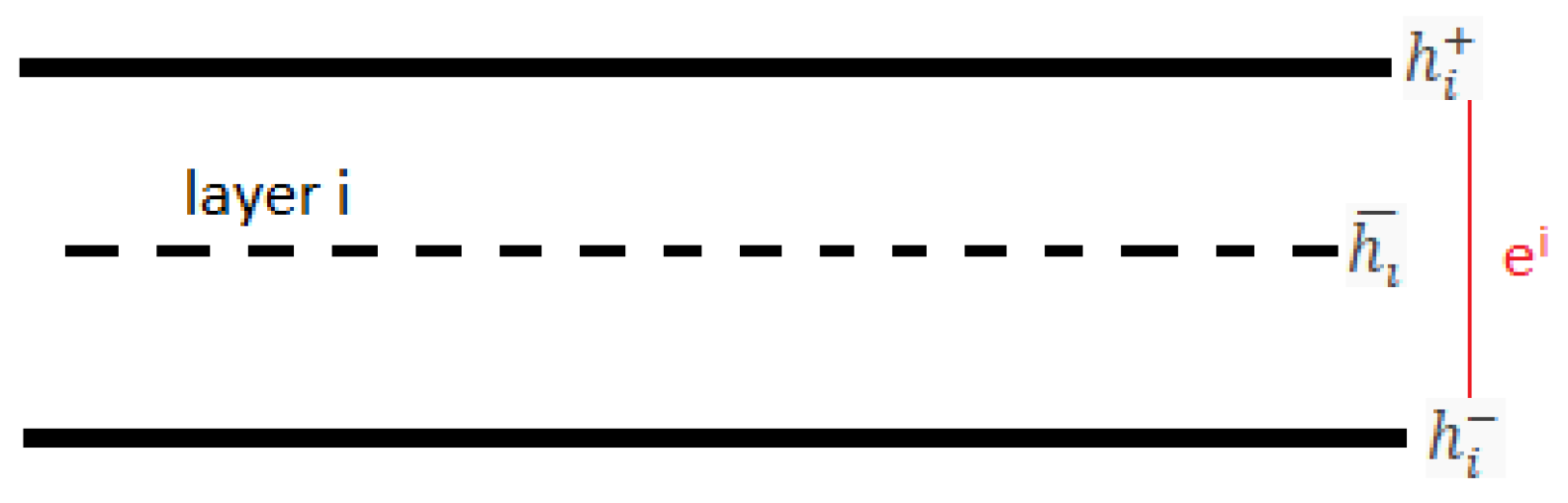
2.1. Notations and Model Description

We consider a linear elastic multilayered plate consisting of n orthotropic elastic layers and occupying the $3D$ domain ${\displaystyle \Omega =\omega \times [h_1^{-},h_n^{+}]}$ where $\omega \subset {\mathbb{R}}^2$ is the middle surface of the plate and h its thickness. The plate is subjected to forces on its upper face ${\omega }^{+}$ and lower face ${\omega }^{-}$ with distributed surface forces ${\displaystyle T^{+}=\left(T_k^{+}\right) \mathrm{and} T^{-}=\left(T_k^{-}\right)}$. The boundary of the domain, denoted by $\partial \Omega$, is decomposed into two parts: a free part ${\displaystyle \partial {\Omega }_N=\partial {\omega }_N\times [h_1^{-},h_n^{+}]}$ where $T=\left(T_k\right)=\left({\sigma }_{kl}{n}_l\right)$ is set to zero, and a restrained part ${\displaystyle \partial {\Omega }_D=\partial {\omega }_D\times [h_1^{-},h_n^{+}]}$ where the displacement $u=\left(u_k\right)$ is set to zero. The subsets $\partial {\omega }_N \mathrm{and} \partial {\omega }_D$ are the partition of $\partial \omega$, and $n=\left(n_k\right)$ is the outer normal of $\partial {\omega }_N$.

In the following, $x \mathrm{and} y$ are the in-plane coordinates and z is the out-of-plane coordinate. The following notations are introduced:

• The subscript $i \mathrm{and} j,j+1$ indicate layer i, and the interface between layers $j \mathrm{and} j+1$ with $1\le i\le n \mathrm{and} 1\le j\le n-1$, respectively. By extension, the superscripts $0,1 \mathrm{and} n,n+1$ refer to the lower face ${\omega }^{-}=\omega \times h_1^{-}$ and the upper face ${\omega }^{+}=\omega \times h_n^{+}$, respectively.
• In each layer $i,h_i^{-},h_i^{+} \mathrm{and} {\overline{h}}_i$ are, respectively, the bottom, the top and the mid-plane z coordinate of the layer, and $e^i=h_i^{+}-h_i^{-}$ is the thickness. Thus, we have $h_i^{+}=h_{i+1}^{-}$ for all $a\le i\le n-1$, and we set $h_0^{+}=h_1^{-} \mathrm{and} h_{n+1}^{-}=h_n^{+}$. See Figure 1.
• Greek subscripts $\alpha ,\beta ,\gamma ,\dots \in \{1,2\}$ indicate the in-plane components.
• Latin subscripts $k,l,m,n,\dots \in \{1,2,3\}$ indicate the $3D$ components.
• ${}^t\left[X\right]$ is the transpose of $\left[X\right]$.
• ${\displaystyle ({\mathit{S}}^i=\left(S_{klmn}^i\right))}$ is the fourth-order 3D compliance tensor of layer i with the minor and major symmetries: $S_{klmn}^i=S_{lkmn}^i=S_{klnm}^i=S_{mnkl}^i$, and it is positive definite. Its inverse is the 3D elasticity stiffness tensor and is denoted by ${\displaystyle \left(C_{klmn}^i\right)}$ for layer i. The tensor ${\displaystyle \left(C_{klmn}^i\right)}$ possesses the same symmetries as ${\displaystyle \left(S_{klmn}^i\right)}$, and it is also positive definite.
• ${\mathit{S}}^i$ is monoclinic in direction z: $S_{\alpha \beta \gamma 3}^i=S_{\alpha 333}^i=0$
• ${\sigma }_{\alpha \beta }(x,y,z)$ are the in-plane stress components, ${\sigma }_{\alpha 3}(x,y,z)$ are the transverse shear stresses and ${\sigma }_{33}(x,y,z)$ is the normal stress.
• ${ϵ}_{\alpha \beta }(x,y,z)$ are the in-plane strain components, ${ϵ}_{\alpha 3}(x,y,z)$ are the transverse strains and ${ϵ}_{33}(x,y,z)$ is the normal strain.
• $u_{\alpha }(x,y,z)$ are the in-plane 3D displacement components, and $u_3(x,y,z)$ is the normal 3D displacement component.

2.2. The 3D Model Equations

The $3D$ elastic problem is to find a statically compatible stress field $\sigma =\left({\sigma }_{kl}\right)$, and a kinematically strain field $ϵ=\left({ϵ}_{kl}\right)$ which comply with the constitutive equation:

$${ϵ}_{kl}\left(x,y,z\right)=S_{klmn}\left(z\right):{\sigma }_{mn}\left(x,y,z\right) \mathrm{on} \Omega ,$$

(1)

where the stress field $\sigma$ is statically compatible if it complies with the equilibrium equations:

$${\sigma }_{kl,l}=0 \mathrm{on} \Omega ,$$

(2)

and the stress conditions on the upper and the lower faces:

$${\sigma }_{k3}=-T_k^{-} \mathrm{on} {\omega }^{-},{\sigma }_{k3}=T_k^{+} \mathrm{on} {\omega }^{+},$$

(3)

and on the lateral boundary:

$${\sigma }_{kl}{n}_l=0 \mathrm{on} \partial {\Omega }_N.$$

(4)

A strain field $ϵ$ is kinematically compatible if there exists a displacement field $\mathit{u}=\left(u_k\right)$ complying with the displacement conditions on the lateral boundary:

$$u_k=0 \mathrm{on} \partial {\Omega }_D,$$

(5)

and such that

$${\displaystyle {ϵ}_{kl}=\frac{1}{2}\left(u_{k,l}+u_{l,k}\right) \mathrm{on} \Omega .}$$

(6)

2.3. The Static of the SCLS1 Model

The SCLS1 model considers the following form of the $3D$ stresses in layer i, for $1\le i\le n$, such that ${\sigma }_{\alpha \beta }$ are layerwise functions of z, the transverse shear stress ${\sigma }_{\alpha 3}$ are layerwise quadratic functions of z, and the normal stress ${\sigma }_{33}$ is a layerwise third-order polynomial function of z. In addition, the stresses ${\sigma }_{\alpha 3} \mathrm{and} {\sigma }_{33}$ take into account the continuity at the interfaces between the layers:

$${\displaystyle {\sigma }_{\alpha \beta }^{3D}(x,y,z)=N_{\alpha \beta }^i(x,y)\frac{P_0^i\left(z\right)}{e^i}+\frac{12}{{e^i}^2}{M}_{\alpha \beta }^i(x,y)P_1^i\left(z\right)}$$

(7)

$$\begin{array}{ccc}{\sigma }_{\alpha 3}^{3D}(x,y,z)& =& {\displaystyle Q_{\alpha }^i\frac{P_0^i\left(z\right)}{e^i}+\left({\mathsf{\tau }}_{\alpha }^{i,i+1}(x,y)-{\mathsf{\tau }}_{\alpha }^{i-1,i}(x,y)\right)P_1^i\left(z\right)}\hfill \\ & +& {\displaystyle \left({\displaystyle Q_{\alpha }^i(x,y)-\frac{e^i}{2}\left({\mathsf{\tau }}_{\alpha }^{i,i+1}(x,y)+{\mathsf{\tau }}_{\alpha }^{i-1,i}(x,y)\right)}\right)\frac{P_2^i\left(z\right)}{e^i}}\hfill \end{array}$$

(8)

$$\begin{array}{ccc}{\sigma }_{33}^{3D}(x,y,z)& =& \left({\displaystyle \frac{1}{2}\left({\nu }^{i,i+1}(x,y)+{\nu }^{i-1,i}(x,y)\right)+\frac{e^i}{12}\left({\pi }^{i,i+1}(x,y)-{\pi }^{i-1,i}(x,y)\right)}\right)P_0^i\left(z\right)\hfill \\ & +& \left({\displaystyle \frac{6}{5}\left({\nu }^{i,i+1}(x,y)-{\nu }^{i-1,i}(x,y)\right)+\frac{e^i}{10}\left({\pi }^{i,i+1}(x,y)+{\pi }^{i-1,i}(x,y)\right)}\right)P_1^i\left(z\right)\hfill \\ & +& \left({\displaystyle \frac{e^i}{12}\left({\pi }^{i,i+1}(x,y)-{\pi }^{i-1,i}(x,y)\right)}\right)P_2^i\left(z\right)\hfill \\ & +& \left({\displaystyle \frac{e^i}{2}\left({\pi }^{i,i+1}(x,y)+{\pi }^{i-1,i}(x,y)\right)+\left({\nu }^{i,i+1}(x,y)-{\nu }^{i-1,i}(x,y)\right)}\right)P_3^i\left(z\right)\hfill \end{array}$$

(9)

where $P_k^i,k=0,1,2,3,$ are the orthogonal Legendre-like polynomial basis defined on layer i by: for $h_i^{-}\le z\le h_i^{+},$

$$\left\{\begin{array}{ccc}{P}_0^i\left(z\right)& =& 1\hfill \\ P_1^i\left(z\right)& =& {\displaystyle \frac{z-{\overline{h}}_i}{e^i}}\hfill \\ P_2^i\left(z\right)& =& {\displaystyle -6{\left({\displaystyle \frac{z-{\overline{h}}_i}{e^i}}\right)}^2+\frac{1}{2}}\hfill \\ P_3^i\left(z\right)& =& {\displaystyle -2{\left({\displaystyle \frac{z-{\overline{h}}_i}{e^i}}\right)}^3+\frac{3}{10}\left({\displaystyle \frac{z-{\overline{h}}_i}{e^i}}\right)}\hfill \end{array}\right.$$

(10)

and where:

• $N^i=\left(N_{\alpha \beta }\right)$ is in-plane stress resultants tensor, related to the $3D$ local stress $\left({\sigma }_{ij}\right)$ in each layer i by:

  $$N^i=(N_{\alpha \beta }^i)=\langle {\sigma }_{\alpha \beta }^{3D}\rangle$$

  where the integration through the thickness is noted ${\displaystyle \langle ·\rangle :{\int }_{h_i^{-}}^{h_i^{+}}f\left(z\right)dz=\langle f\rangle .}$
• $M^i=\left(M_{\alpha \beta }\right)$ is the moment resultants tensor expressed in terms of the $3D$ stress field ${\sigma }^{3D}$ in each layer i as follows:

  $$M^i=(M_{\alpha \beta }^i)=\langle (z-{\overline{h}}_i){\sigma }_{\alpha \beta }^{3D}\rangle$$
• $Q^i=\left(Q_{\alpha }^i\right)$ is the out-of-plane shear stress resultant vector, defined from the $3D$ stress field ${\sigma }^{3D}$ in each layer i as follows:

  $$Q^i=\left(Q_{\alpha }^i\right)=\langle {\sigma }_{\alpha 3}^{3D}\rangle$$
• ${\tau }_{\alpha }^{j,j+1}$ is the interlaminar shear stress at the interface between layer j, and layer $j+1$ for $0\le j\le n-1$ given by:

  $${\tau }_{\alpha }^{j,j+1}(x,y)={\sigma }_{\alpha 3}^{3D}(x,y,h_j^{+})={\sigma }_{\alpha 3}^{3D}(x,y,h_{j+1}^{-})$$
• ${\nu }^{j,j+1}$ is the normal stress at the interface between j and $j+1$, for $0\le j\le n-1$, given by:

  $${\nu }^{j,j+1}(x,y)={\sigma }_{33}^{3D}(x,y,h_j^{+})={\sigma }_{33}^{3D}(x,y,h_{j+1}^{-})$$
• ${\pi }^{j,j+1}$ is the divergence of the interlaminar shear stress vector ${\tau }^{j,j+1}=\left({\tau }_{\alpha }^{j,j+1}\right)$ defined on the interface between layer j and $j+1$ for $0\le j\le n-1$.

2.4. The Equilibrium Equations

The ${\sigma }^{3D}$ will verify the $3D$ equilibrium Equation $\left(2\right)$, if and only if:

$$\left\{\begin{array}{ccc}& & N_{\alpha \beta ,\beta }^i+{\tau }_{\alpha }^{i,i+1}-{\tau }_{\alpha }^{i-1,i}=0\hfill \\ & & Q_{\alpha ,\alpha }^i+{\nu }^{i,i+1}-{\nu }^{i-1,i}=0\hfill \\ & & {\displaystyle M_{\alpha \beta ,\beta }-Q_{\alpha }+\frac{e^i}{2}\left({\tau }_{\alpha }^{i,i+1}+{\tau }_{\alpha }^{i-1,i}\right)=0}\hfill \\ & & {\tau }_{\alpha ,\alpha }^{j,j+1}-{\pi }^{j,j+1}=0\hfill \end{array}\right.\mathrm{in}\omega$$

(11)

for all $i=1,\dots ,n \mathrm{and} j=0,\dots ,n$.

The lateral boundary conditions ${\sigma }_{ij}^{3D}{n}_j=0$ on $\partial {\Omega }_N$ are equivalent to the following equations $i=1,\dots ,n \mathrm{and} j=0,\dots ,n:$

$$N_{\alpha \beta }^i{n}_{\beta }=0,M_{\alpha \beta }^i{n}_{\beta }=0,Q_{\alpha }{n}_{\alpha }^i=0,{\tau }_{\alpha }^{j,j+1}{n}_{\alpha }=0 \mathrm{on} \partial {\omega }_N$$

(12)

whereas in-plane traction continuity is equivalent to continuity of the generalized tractions involved in (12).

In addition, the boundary conditions on the lower and the upper faces write, respectively,

$$\left\{\begin{array}{ccc}{\tau }_1^{0,1}(x,y)& =& -T_1^{-}(x,y)\hfill \\ {\tau }_2^{0,1}(x,y)& =& -T_2^{-}(x,y)\hfill \\ {\nu }^{0,1}(x,y)& =& -T_3^{-}(x,y)\hfill \end{array}\right.$$

(13)

$$\left\{\begin{array}{ccc}{\tau }_1^{n,n+1}(x,y)& =& T_1^{+}(x,y)\hfill \\ {\tau }_2^{n,n+1}(x,y)& =& T_2^{+}(x,y)\hfill \\ {\nu }^{n,n+1}(x,y)& =& T_3^{+}(x,y)\hfill \end{array}\right.$$

(14)

2.5. Generalized Displacements

The SCLS1 generalized displacements are $(U_{\alpha }^i,U_3^i,{\Phi }_{\alpha }^i \mathrm{and} V^{j,j+1})$. $U_{\alpha }^i$ are the two in-plane displacements, $U_3^i$ is the vertical displacement, ${\Phi }_{\alpha }^i$ are the two bending rotations in each layer i, and $V^{j,j+1}$ is a kinematical variable, having the dimension of an area, which is dual to the static variable ${\pi }^{j,j+1}$ defined on the interface $j,j+1$:

$${\displaystyle U_{\alpha }^i(x,y)={\int }_{h_i^{-}}^{h_i^{+}}{\displaystyle \frac{P_0^i\left(z\right)}{e^i}{u}_{\alpha }(x,y,z)dz}}$$

(15)

$${\displaystyle {\Phi }_{\alpha }^i(x,y)={\int }_{h_i^{-}}^{h_i^{+}}{\displaystyle \frac{12}{{e^i}^2}{P}_1^i\left(z\right)u_{\alpha }(x,y,z)dz}}$$

(16)

$${\displaystyle U_3^i(x,y)={\int }_{h_i^{-}}^{h_i^{+}}\left({\displaystyle \frac{P_0^i\left(z\right)}{e^i}+\frac{P_2^i\left(z\right)}{e^i}}\right)u_3(x,y,z)dz}$$

(17)

$${\displaystyle W_{\pm }^i(x,y)={\int }_{h_i^{-}}^{h_i^{+}}\left({\displaystyle P_1^i\left(z\right)\pm \frac{P_2^i\left(z\right)}{2}}\right)u_3(x,y,z)dz}$$

(18)

and,

$$V^{j,j+1}(x,y)=W_{-}^j(x,y)-W_{+}^{j+1}(x,y)$$

(19)

In addition, the generalized displacement verifies the following generalized boundary conditions for $1\le i\le n$ and $0\le j\le n$:

$$U_{\alpha }^i=0,U_3^i=0,{\Phi }_{\alpha }^i=0,V^{j,j+1}=0, \mathrm{on} \partial {\omega }_D.$$

(20)

2.6. Generalized Strains

The generalized strains dual of the generalized stresses $N_{\alpha \beta }^i,M_{\alpha \beta }^i,{\tau }_{\alpha }^{j,j+1},{\nu }^{j,j+1},{\pi }^{j,j+1}$ for $i=1,\dots ,n \mathrm{and} j=1,\dots ,n-1$ are respectively expressed in terms of the generalized displacements as:

$${\displaystyle \begin{array}{ccc}{ϵ}_{\alpha \beta }^i& =& {\displaystyle \frac{1}{2}\left(U_{\alpha ,\beta }^i+U_{\beta ,\alpha }^i\right)}\hfill \\ {\chi }_{\alpha \beta }^i& =& \frac{1}{2}\left({\Phi }_{\alpha ,\beta }^i+{\Phi }_{\beta ,\alpha }^i\right)\hfill \\ {\gamma }_{\alpha }^i& =& {\Phi }_{\alpha }^i+U_{3,\alpha }^i\hfill \\ D_{\alpha }^{j,j+1}& =& U_{\alpha }^{j+1}-U_{\alpha }^j-\frac{e^j}{2}{\Phi }_{\alpha }^j-\frac{e^{j+1}}{2}{\Phi }_{\alpha }^{j+1}\hfill \\ D_v^{j,j+1}& =& U_3^{j+1}-U_3^j,\hfill \\ {\lambda }^{j,j+1}& =& V^{j,j+1}\hfill \end{array}}$$

2.7. The Constitutive Equations of the SCLS1 Model

The constitutive equations of the SCLS1 model are calculated using the stress energy associated with ${\sigma }^{3D}$. They are given by: for $1\le i\le n \mathrm{and} \mathrm{for} 1\le j\le n-1$

• Membrane constitutive equation of layer i:

  $${\displaystyle {ϵ}_{\alpha \beta }^i=\frac{1}{e^i}{S}_{\alpha \beta \gamma \delta }^i{N}_{\gamma \delta }^i+S_{\alpha \beta 33}^i\left({\displaystyle \frac{1}{2}\left({\nu }^{i,i+1}+{\nu }^{i-1,i}\right)+\frac{e^i}{12}\left({\pi }^{i,i+1}-{\pi }^{i-1,i}\right)}\right).}$$

  (21)
• Bending constitutive equations of layer i:

  $${\displaystyle {\chi }_{\alpha \beta }^i=\frac{12}{{e^i}^3}{S}_{\alpha \beta \gamma \delta }^i{M}_{\gamma \delta }^i+\frac{1}{e^i}{S}_{\alpha \beta 33}^i\left({\displaystyle \frac{6}{5}\left({\nu }^{i,i+1}-{\nu }^{i-1,i}\right)+\frac{e^i}{10}\left({\pi }^{i,i+1}+{\pi }^{i-1,i}\right)}\right).}$$

  (22)
• Transverse shear constitutive equation of layer i:

  $${\displaystyle {\gamma }_{\alpha }^i=\frac{24}{5e^i}{S}_{\alpha 3\beta 3}^i{Q}_{\beta }^i-\frac{2}{5}{S}_{\alpha 3\beta 3}^i({\mathsf{\tau }}_{\beta }^{i,i+1}+{\mathsf{\tau }}_{\beta }^{i-1,i}).}$$

  (23)
• Shear constitutive equation of interface $j,j+1$:

  $$\begin{array}{ccc}{D}_{\alpha }^{j,j+1}& =& {\displaystyle -\frac{2}{5}{S}_{\alpha 3\beta 3}^j{Q}_{\beta }^j-\frac{2}{5}{S}_{\alpha 3\beta 3}^{j+1}{Q}_{\beta }^{j+1}-\frac{2}{15}{e}^j{S}_{\alpha 3\beta 3}^j{\mathsf{\tau }}_{\beta }^{j-1,j}}\hfill \\ & & {\displaystyle +\frac{8}{15}{\mathsf{\tau }}_{\beta }^{j,j+1}\left(e^j{S}_{\alpha 3\beta 3}^j+e^{j+1}{S}_{\alpha 3\beta 3}^{j+1}\right)-\frac{2}{15}{e}^{j+1}{S}_{\alpha 3\beta 3}^{j+1}{\mathsf{\tau }}_{\beta }^{j+1,j+2}.}\hfill \end{array}$$

  (24)
• Normal constitutive equation of interface $j,j+1$:

  $$\begin{array}{ccc}{D}_{\nu }^{j,j+1}& =& {\displaystyle \frac{9}{70}{e}^j{S}_{3333}^j{\nu }^{j-1,j}+\frac{13}{35}\left(e^j{S}_{3333}^j+e^{j+1}{S}_{3333}^{j+1}\right){\nu }^{j,j+1}}\hfill \\ & & {\displaystyle +\frac{9}{70}{e}^{j+1}{S}_{3333}^{j+1}{\nu }^{j+1,j+2}-\frac{13}{420}{\left(e^j\right)}^2{S}_{3333}^j{\pi }^{j-1,j}}\hfill \\ & & {\displaystyle +\frac{11}{210}\left({\left(e^j\right)}^2{S}_{3333}^j-{\left(e^{j+1}\right)}^2{S}_{3333}^{j+1}\right){\pi }^{j,j+1}}\hfill \\ & & {\displaystyle +\frac{13}{420}{\left(e^{j+1}\right)}^2{S}_{3333}^{j+1}{\pi }^{j+1,j+2}+\frac{1}{2}{S}_{\alpha \beta 33}^j{N}_{\alpha \beta }^j.}\hfill \\ & & {\displaystyle +\frac{1}{2}{S}_{\alpha \beta 33}^{j+1}{N}_{\alpha \beta }^{j+1}+\frac{6}{5e^j}{S}_{\alpha \beta 33}^j{M}_{\alpha \beta }^j-\frac{6}{5e^{j+1}}{S}_{\alpha \beta 33}^{j+1}{M}_{\alpha \beta }^{j+1}.}\hfill \end{array}$$

  (25)
• Constitutive equation for the $\pi$ generalized stress at interface $j,j+1$:

  $$\begin{array}{ccc}{\lambda }^{j,j+1}& =& {\displaystyle \frac{1}{105}\left(S_{3333}^j{\left(e^j\right)}^3+{\left(e^{j+1}\right)}^3{S}_{3333}^{j+1}\right){\pi }^{j,j+1}-\frac{1}{140}{S}_{3333}^j{\left(e^j\right)}^3{\pi }^{j-1,j}}\hfill \\ & & {\displaystyle -\frac{1}{140}{\left(e^{j+1}\right)}^3{S}_{3333}^{j+1}{\pi }^{j+1,j+2}+\frac{11}{210}{\nu }^{j,j+1}\left({\left(e^j\right)}^2{S}_{3333}^j-{\left(e^{j+1}\right)}^2{S}_{3333}^{j+1}\right)}\hfill \\ & & {\displaystyle +\frac{13}{420}{\left(e^j\right)}^2{S}_{3333}^j{\nu }^{j-1,j}-\frac{13}{420}{\left(e^{j+1}\right)}^2{S}_{3333}^{j+1}{\nu }^{j+1,j+2}}\hfill \\ & & {\displaystyle +\frac{e^j}{12}{S}_{\alpha \beta 33}^j{N}_{\alpha \beta }^j-\frac{e^{j+1}}{12}{S}_{\alpha \beta 33}^{j+1}{N}_{\alpha \beta }^{j+1}+\frac{1}{10}{S}_{\alpha \beta 33}^j{M}_{\alpha \beta }^j+\frac{1}{10}{S}_{\alpha \beta 33}^{j+1}{N}_{\alpha \beta }^{j+1}.}\hfill \end{array}$$

  (26)

2.8. Finite-Element Displacement-Based Implementation

The numerical study of the SCLS1 multilayered plate model has been investigated in [36] using an in-house FE solver described in [30], and in [38] using the open-source finite element FEniCS package [39,40]. This latter implementation follows a classical finite-element interpolation of the generalized displacement fields. In particular, all kinematic variables $U_{\alpha }^i,U_3^i,{\Phi }_{\alpha }^i$ and $V^{j,j+1}$ are interpolated as a quadratic polynomial on a triangular cell of a 2D mesh. As discussed in [36,39], the finite-element discretization suffers from shear-locking issues in the thin plate limit, which is alleviated using selective reduced integration.

3. Hybridized Mixed Methods for 3D Continua

Mixed approaches for 3D continua consist of considering a simultaneous interpolation for the stress variable $\sigma$ and the displacement u [41,42,43,44]. The interpolation space for $\sigma$ is often chosen to satisfy the traction continuity condition. If choosing such spaces is feasible when u is a scalar (e.g., in the case of antiplane elasticity), this is much harder for the general vectorial case of 2D/3D elasticity [45,46,47]. Hybridized mixed methods therefore consist of relaxing the a priori traction continuity requirement and including it in the variational formulation [48]. They are therefore easier to formulate, especially regarding the choice of the stress interpolation space, and offer computational advantages as it will be seen in the following section.

3.1. Continuous Variational Formulation

Let us consider a domain $\Omega$ with imposed displacements $u_i=u_i^0$ on a Dirichlet part $\partial {\Omega }_D$ of the boundary and imposed tractions ${\sigma }_{ij}{n}_j=T_i^0$ on the remaining Neumann part $\partial {\Omega }_N=\partial \Omega \mathit{\setminus }\partial {\Omega }_D$. Let us also denote by $\Gamma$ the set of internal lines of stress discontinuities (typically inner edges of a finite-element mesh) and introduce the jump operator through $\Gamma$ as follows: $\left[\left[v\right]\right]=v^{+}+v^{-}$ where ± are arbitrarily defined sides of $\Gamma$. $n^{+}$ (resp. $n^{-}$) will denote the unit normal of $\Gamma$ pointing outwards of the + (resp. −) side.

Let us start from the complementarity energy principle which states that the solution (in terms of stresses) minimizes the following complementarity energy under static equilibrium conditions:

$$\begin{array}{cc}\hfill {\displaystyle \underset{\sigma }{min}}& {\displaystyle {\int }_{\Omega }{\displaystyle \frac{1}{2}}{\sigma }_{ij}{S}_{ijkl}{\sigma }_{kl}d\Omega -{\int }_{\partial {\Omega }_D}{\sigma }_{ij}{n}_j{u}_i^{0}dS}\hfill \\ \hfill \mathrm{s}.\mathrm{t}.& {\sigma }_{ij,j}+f_i=0\mathrm{in}\Omega \hfill \\ \hfill & \left[\left[{\sigma }_{ij}{n}_j\right]\right]=0\mathrm{on}\Gamma \hfill \\ \hfill & {\sigma }_{ij}{n}_j=T_i^0\mathrm{on}\partial {\Omega }_N\hfill \end{array}$$

(27)

Introducing a Lagrange multiplier u defined on $\Omega$ associated with the first constraint, and another Lagrange multiplier v defined on $\Gamma \cup \partial {\Omega }_N$ associated with the last two constraints, the above minimization problem is equivalent to the following saddle point problem:

$$\underset{u,v}{max}\underset{\sigma }{min}\mathcal{L}(\sigma ,u,v)$$

(28)

where the system Lagrangian is given by:

$$\begin{array}{cc}\hfill \mathcal{L}(\sigma ,u,v)=& {\int }_{\Omega }{\displaystyle \frac{1}{2}}{\sigma }_{ij}{S}_{ijkl}{\sigma }_{kl}d\Omega -{\int }_{\partial {\Omega }_D}{\sigma }_{ij}{n}_j{u}_i^{0}dS\hfill \\ \hfill & +{\int }_{\Omega }({\sigma }_{ij,j}+f_i)u_{i}d\Omega \hfill \\ \hfill & +{\int }_{\Gamma }\left[\left[{\sigma }_{ij}{n}_j\right]\right]v_{i}dS+{\int }_{\partial {\Omega }_N}({\sigma }_{ij}{n}_j-T_i^0)v_{i}dS\hfill \end{array}$$

(29)

The first-order optimality conditions of this min/max result in the following mixed variational formulation: Find $(\sigma ,u,v)\in {\mathcal{V}}_{\sigma }\times {\mathcal{V}}_u\times {\mathcal{V}}_v$ such that:

$$\begin{array}{cc}& {\int }_{\Omega }{\widehat{\sigma }}_{ij}{S}_{ijkl}{\sigma }_{kl}d\Omega +{\int }_{\Omega }{\sigma }_{ij,j}{u}_{i}d\Omega \hfill \\ \hfill +& {\int }_{\Gamma }\left[\left[{\widehat{\sigma }}_{ij}{n}_j\right]\right]v_{i}dS+{\int }_{\partial {\Omega }_N}{\widehat{\sigma }}_{ij}{n}_j{v}_{i}dS\hfill & ={\int }_{\partial {\Omega }_D}{\widehat{\sigma }}_{ij}{n}_j{u}_i^{0}dS\hfill & \hfill \forall \widehat{\sigma }\in {\mathcal{V}}_{\sigma }\end{array}$$

(30)

$$\begin{array}{ccc}\hfill {\int }_{\Omega }{\sigma }_{ij,j}{\widehat{u}}_{i}d\Omega & =-{\int }_{\Omega }{f}_i{\widehat{u}}_{i}d\Omega \hfill & \hfill \forall \widehat{u}\in {\mathcal{V}}_u\end{array}$$

(31)

$$\begin{array}{ccc}\hfill {\int }_{\Gamma }\left[\left[{\sigma }_{ij}{n}_j\right]\right]{\widehat{v}}_{i}dS+{\int }_{\partial {\Omega }_N}{\sigma }_{ij}{n}_j{\widehat{v}}_{i}dS& ={\int }_{\partial {\Omega }_N}{T}_i^0{\widehat{v}}_{i}dS\hfill & \hfill \forall \widehat{v}\in {\mathcal{V}}_v\end{array}$$

(32)

where ${\mathcal{V}}_{\sigma }$, ${\mathcal{V}}_u$ and ${\mathcal{V}}_v$ are appropriate function spaces for the corresponding variable.

Let us introduce the following notations for the different bilinear forms:

$$\begin{array}{cc}\hfill a(\widehat{\sigma },\sigma )& :={\int }_{\Omega }{\widehat{\sigma }}_{ij}{S}_{ijkl}{\sigma }_{kl}d\Omega \hfill \\ \hfill b(\widehat{\sigma },u)& :={\int }_{\Omega }{\widehat{\sigma }}_{ij,j}{u}_{i}d\Omega \hfill \\ \hfill c(\widehat{\sigma },v)& :={\int }_{\Gamma }\left[\left[{\widehat{\sigma }}_{ij}{n}_j\right]\right]v_{i}dS+{\int }_{\partial {\Omega }_N}{\widehat{\sigma }}_{ij}{n}_j{v}_{i}dS\hfill \end{array}$$

and:

$$\begin{array}{cc}\hfill {\ell }_1\left(\widehat{\sigma }\right)& :={\int }_{\partial {\Omega }_D}{\widehat{\sigma }}_{ij}{n}_j{u}_i^{0}dS\hfill \\ \hfill {\ell }_2\left(\widehat{u}\right)& :=-{\int }_{\Omega }{f}_i{\widehat{u}}_{i}d\Omega \hfill \\ \hfill {\ell }_3\left(\widehat{v}\right)& :={\int }_{\partial {\Omega }_N}{T}_i^0{\widehat{v}}_{i}dS\hfill \end{array}$$

for the different linear forms, such that the variational formulation can be rewritten as:

$$\begin{array}{cccc}a(\widehat{\sigma },\sigma )+b(\widehat{\sigma },u)+c(\widehat{\sigma },v)\hfill & =& {\ell }_1\left(\widehat{\sigma }\right)\hfill & \forall \widehat{\sigma }\in {\mathcal{V}}_{\sigma }\hfill \\ b(\sigma ,\widehat{u})\hfill & =& {\ell }_2\left(\widehat{u}\right)\hfill & \forall \widehat{u}\in {\mathcal{V}}_u\hfill \\ c(\sigma ,\widehat{v})\hfill & =& {\ell }_3\left(\widehat{v}\right)\hfill & \forall \widehat{v}\in {\mathcal{V}}_v\hfill \end{array}$$

(33)

The above symmetric block-like structure is typical of hybrid mixed methods. Let us note that, from a mechanical stand point, u and v can both be interpreted as displacements, defined either in $\Omega$ or on $\Gamma \cup \partial {\Omega }_N$. Finally, no continuity conditions across $\Gamma$ are required for both $\sigma$ and u.

3.2. Finite-Element Discretization

Let us now consider a discretization of $\Omega$ into a mesh of triangular/tetrahedral cells K and with $\Gamma$ denoting now the inner facets (segments in 2D, triangles in 3D) of this mesh. It is important to point out that no continuity conditions have to be enforced on the stress variable $\sigma$ and the Lagrange multiplier u across the mesh cells. They are both defined cell-wise. The Lagrange multiplier v lives on the mesh facets and is not defined inside the cells. No continuity at the mesh vertices (in 2D) or edges (in 3D) linking different facets are required.

As a result, let us consider a discretization of the stress field $\sigma$ using discontinuous Lagrange elements of degree p for $p\ge 1$ (see also Figure 2). Enforcing the local balance equation will therefore require an interpolation of the Lagrange multiplier field u using discontinuous Lagrange elements of degree $p-1$. Similarly, stress continuity can be achieved using discontinuous Lagrange elements on the facets of degree p for the multiplier field v.

Using standard finite-element technology, the various bilinear/linear forms involved in (33) are assembled into global matrices/vectors forming the following final linear system:

$$\left[\begin{array}{ccc}\mathbf{A}& \mathbf{B}& \mathbf{C}\\ {\mathbf{B}}^T& 0& 0\\ {\mathbf{C}}^T& 0& 0\end{array}\right]\left\{\begin{array}{c}\Sigma \\ U\\ V\end{array}\right\}=\left\{\begin{array}{c}{L}_1\\ L_2\\ L_3\end{array}\right\}$$

(34)

The main feature of hybridizable mixed methods is that operators $\mathbf{A}$ and $\mathbf{B}$ have a block structure since their assembly on each cell involves only stress $\sigma$ and displacement u variables associated with the cell itself. Both $\sigma$ and u can therefore be eliminated by local static condensation at the cell level by inverting a small-size matrix. Doing so, the final system is of a much smaller size than (34) since it involves only the vector of unknowns V corresponding to the Lagrange multiplier v:

$$\tilde{\mathbf{A}}V=L$$

(35)

where $\tilde{\mathbf{A}}$ and L are assembled from the corresponding local contribution of cell K:

$$\begin{array}{cc}\hfill {\tilde{\mathbf{A}}}_K& =-\left[\begin{array}{cc}{\mathbf{C}}_K^T& 0\end{array}\right]{\left[\begin{array}{cc}{\mathbf{A}}_K& {\mathbf{B}}_K\\ {\mathbf{B}}_K^T& 0\end{array}\right]}^{-1}\left[\begin{array}{c}{\mathbf{C}}_K\\ 0\end{array}\right]\hfill \end{array}$$

(36)

$$\begin{array}{cc}\hfill L_K& ={\left(L_3\right)}_K-\left[\begin{array}{cc}{\mathbf{C}}_K^T& 0\end{array}\right]{\left[\begin{array}{cc}{\mathbf{A}}_K& {\mathbf{B}}_K\\ {\mathbf{B}}_K^T& 0\end{array}\right]}^{-1}\left[\begin{array}{c}{\left(L_1\right)}_K\\ {\left(L_2\right)}_K\end{array}\right]\hfill \end{array}$$

(37)

A last interesting feature of hybridized mixed solutions is related to the reconstruction of a displacement field. One simple strategy is to exploit the Lagrange multiplier field u, which gives a piecewise polynomial approximation of the real displacement. Projection of u onto a suitable continuous functional space will therefore give a continuous approximation to the displacement. However, as discussed in [42], the facet Lagrange multiplier v can also be used to derive an even more accurate approximation of the displacement. Such a reconstruction requires the resolution of local problems at the cell-level, the so-obtained displacement usually being non-conforming with continuity at the edge Gauss points. This more advanced reconstruction procedure will not be investigated in this work.

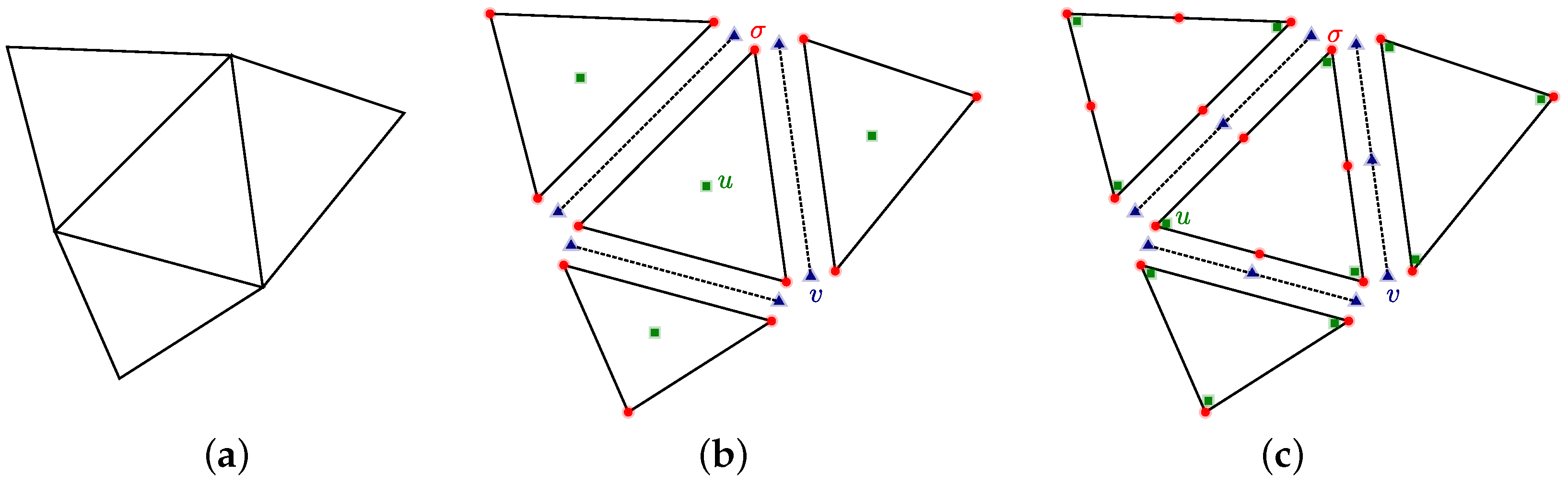
4. Hybridization of a Mixed Method for the SCLS1 Model

In this section, we transpose the hybridization of mixed methods as described in the 3D continuum case to the SCLS1 model.

4.1. Continuous Formulation

Let us first denote by $\Sigma$ the vector of generalized stresses of the SCLS1 model as described in Section 2.3.

The set of equilibrium Equation (11) will be denoted by $\mathcal{D}\Sigma =f$, where $\mathcal{D}$ is the corresponding linear differential operator and f is related to the imposed values $T_{\alpha }^{\pm },T_3^{\pm }$ of ${\tau }_{\alpha }$ and $\nu$ on the top and bottom interfaces as in (20). Similarly to the 3D continuum, two Lagrange multiplier fields will be introduced. These fields are denoted by U and V and will be respectively used to enforce the generalized equilibrium Equation (11) and the continuity and stress boundary conditions associated with (12). The latter conditions will be denoted as follows:

$$\begin{array}{cc}\hfill \left[\right[\mathcal{T}\Sigma \left]\right]=0& \mathrm{on}\Gamma \hfill \end{array}$$

(38)

$$\begin{array}{cc}\hfill \mathcal{T}\Sigma =0& \mathrm{on}\partial {\omega }_N\hfill \end{array}$$

(39)

Finally, introducing $\mathbf{S}$, the generalized compliance matrix involved in the generalized constitutive Equations (21)–(26), the complementary energy principle characterizing the solution to the elastic SCLS1 model can be stated as:

$$\begin{array}{cc}\hfill {\displaystyle \underset{\Sigma }{min}}& {\displaystyle {\int }_{\omega }{\displaystyle \frac{1}{2}}{\Sigma }^T\mathbf{S}\Sigma d\omega }\hfill \\ \hfill \mathrm{s}.\mathrm{t}.& \mathcal{D}\Sigma =f\mathrm{in}\omega \hfill \\ \hfill & \left[\right[\mathcal{T}\Sigma \left]\right]=0\mathrm{on}\Gamma \hfill \\ \hfill & \mathcal{T}\Sigma =0\mathrm{on}\partial {\Omega }_N\hfill \end{array}$$

(40)

in which we considered purely homogeneous Dirichlet and Neumann boundary conditions for simplicity.

The SCLS1 mixed approach will be therefore given by:

$$\begin{array}{cccc}a(\widehat{\Sigma },\Sigma )+b(\widehat{\Sigma },U)+c(\widehat{\Sigma },V)\hfill & =& 0\hfill & \forall \widehat{\Sigma }\in {\mathcal{V}}_{\Sigma }\hfill \\ b(\Sigma ,\widehat{U})\hfill & =& \ell \left(\widehat{U}\right)\hfill & \forall \widehat{U}\in {\mathcal{V}}_U\hfill \\ c(\Sigma ,\widehat{V})\hfill & =& 0\hfill & \forall \widehat{V}\in {\mathcal{V}}_V\hfill \end{array}$$

(41)

where:

$$\begin{array}{cc}\hfill a(\widehat{\Sigma },\Sigma )& :={\int }_{\omega }{\widehat{\Sigma }}^T\mathbf{S}\Sigma d\omega \hfill \\ \hfill b(\widehat{\Sigma },U)& :={\int }_{\omega }{(\mathcal{D}\widehat{\Sigma })}^{T}Ud\omega \hfill \\ \hfill c(\widehat{\Sigma },V)& :={\int }_{\Gamma }{([[\mathcal{T}\widehat{\Sigma }]])}^{T}VdS+{\int }_{\partial {\Omega }_N}{(\mathcal{T}\widehat{\Sigma })}^{T}VdS\hfill \\ \hfill \ell (\widehat{U})& :={\int }_{\omega }{f}^T\widehat{U}d\omega \hfill \end{array}$$

4.2. Finite-Element Implementation

Throughout this study, we will consider the following discretization strategy for the hybridizable mixed approach on a triangular mesh:

• discontinuous Lagrange interpolation of degree p for $\Sigma$;
• discontinuous Lagrange interpolation of degree $p-1$ for U;
• discontinuous Lagrange interpolation of degree p on edges for V;

with either $p=1$ or $p=2$ in the subsequent numerical examples.

This choice is similar to the 3D continuum case although it is not obvious that this choice will be numerically stable. Let us mention that we will not necessarily expect similar stability results as in the 3D continuum case since the generalized differential operator $\mathcal{D}$ couples the various generalized stress fields of $\Sigma$ through first-order and zero-order derivatives as seen in Equation (11). Numerical analysis of the chosen discretization for the SCLS1 model is out of the scope of the present paper and stability will only be assessed numerically in the next section.

However, the discontinuous nature of the chosen interpolations will make it possible to reduce the system at the cell level through local static condensation as discussed in the 3D case. The final reduced system also involves only the Lagrange multiplier field V.

Table 1. Number of degrees of freedom per cell for both mixed discretizations and a pure displacement approach. Each vertex dof counts for $\frac{1}{6}$ in a cell and each edge dof for $\frac{1}{2}$ in the asymptotic fine mesh regime. Total and condensed numbers of dofs are approximated for large values of n.

Discretization	$\mathbf{\Sigma }$	U	V	Total	Condensed
Mixed ($p=1$)	$3(12n-4)$	$6n-1$	$2\frac{3}{2}(6n-1)$	$\approx 60n$	$\approx 18n$
Mixed ($p=2$)	$6(12n-4)$	$3(6n-1)$	$3\frac{3}{2}(6n-1)$	$\approx 117n$	$\approx 27n$
Displacement	–	–	–	$2(6n-1)\approx 12n$

enumerates the total number of degrees of freedom per triangular cell with and without static condensation. We also compare the resulting size with a displacement-based interpolation using continuous quadratic Lagrange triangles for the generalized displacement field as in [36,38]. Clearly, static condensation is absolutely necessary to obtain a reasonable dof count for the mixed approach. For example, for $p=2$ and for 5 layers, without static condensation, there would be around 600 dofs/triangle against 135 with static condensation. It can also be observed that both mixed approaches with static condensation are more expensive than the quadratic displacement approach of [36,38].

Numerical implementation has been performed using the Firedrake software package [49]. The local static condensation operations are performed automatically using the Slate domain-specific language [48]. We used a recent version of Firedrake which relies on Loopy [50] for an optimized assembly of matrix-free local finite-element kernels [51,52].

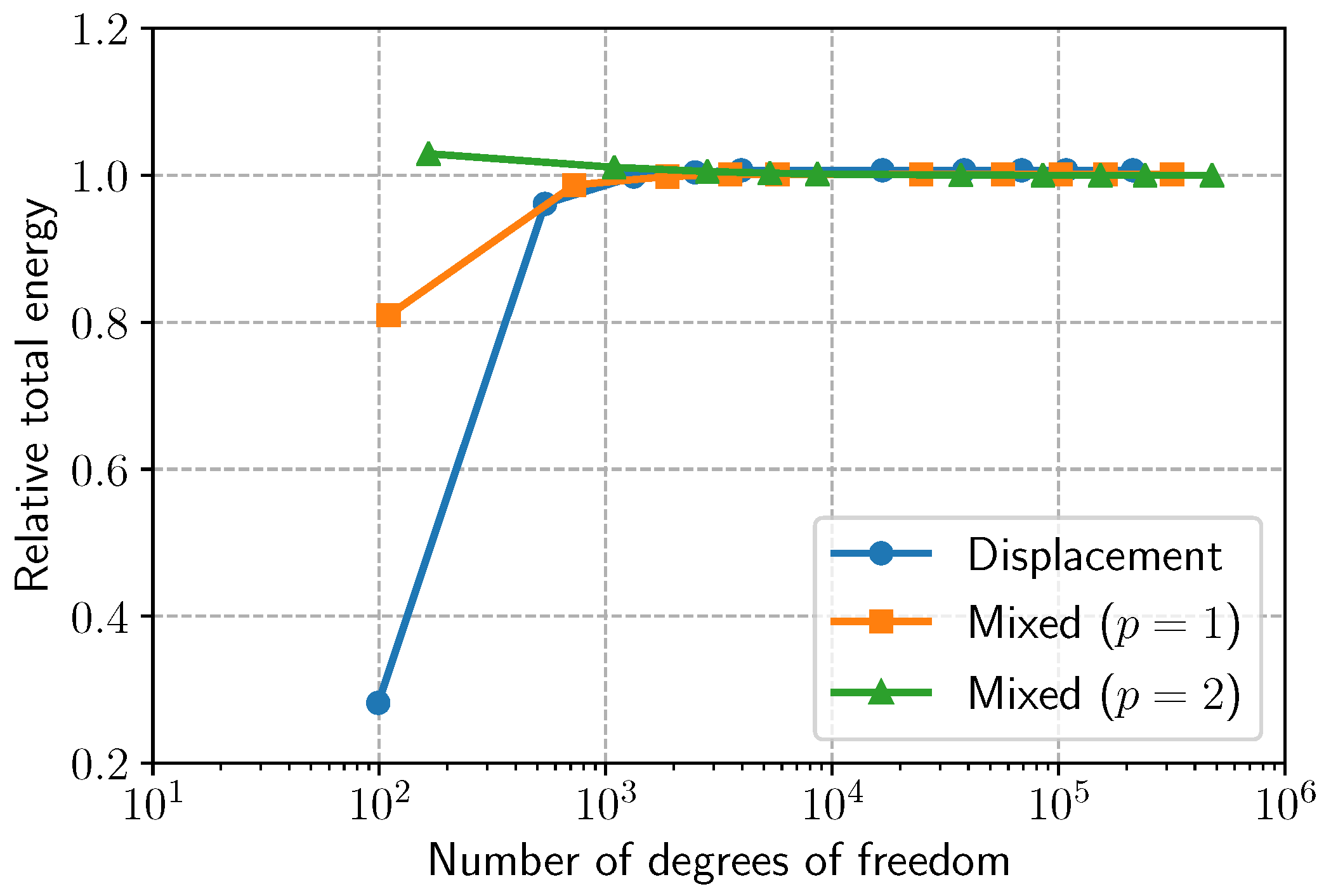
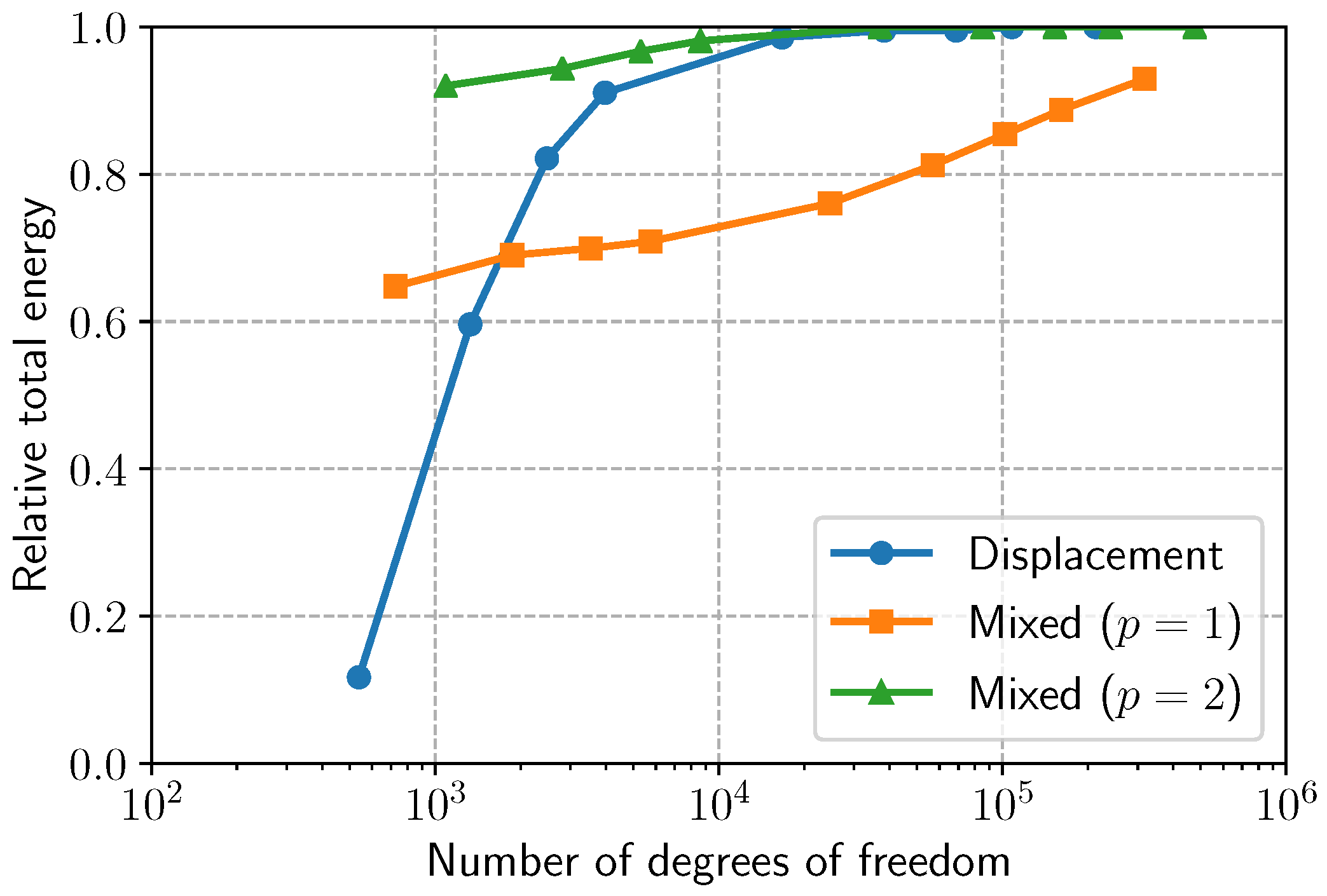
5. Illustrative Applications

In this section, we investigate different illustrative applications assessing the quality of the hybridized mixed approach.

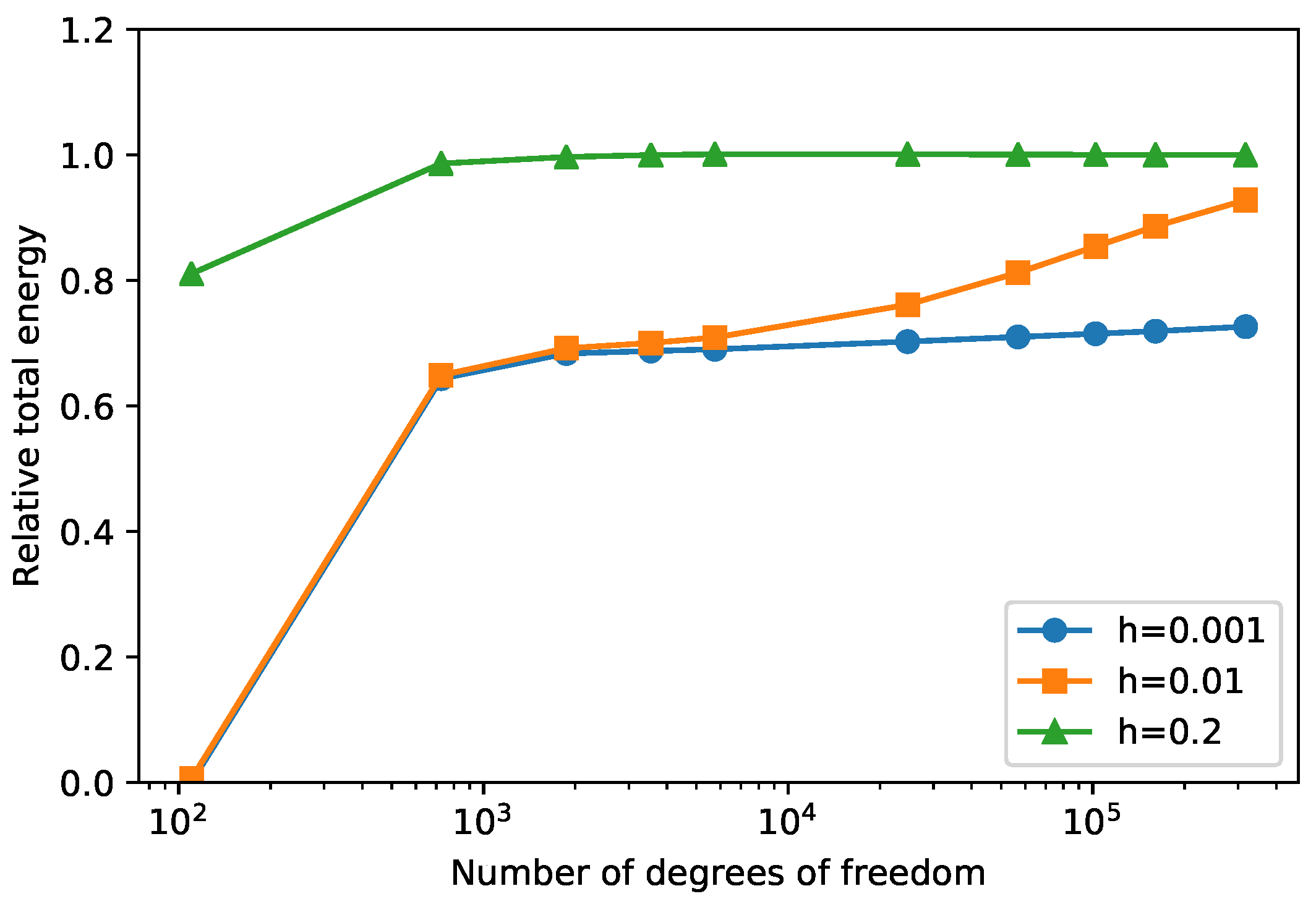
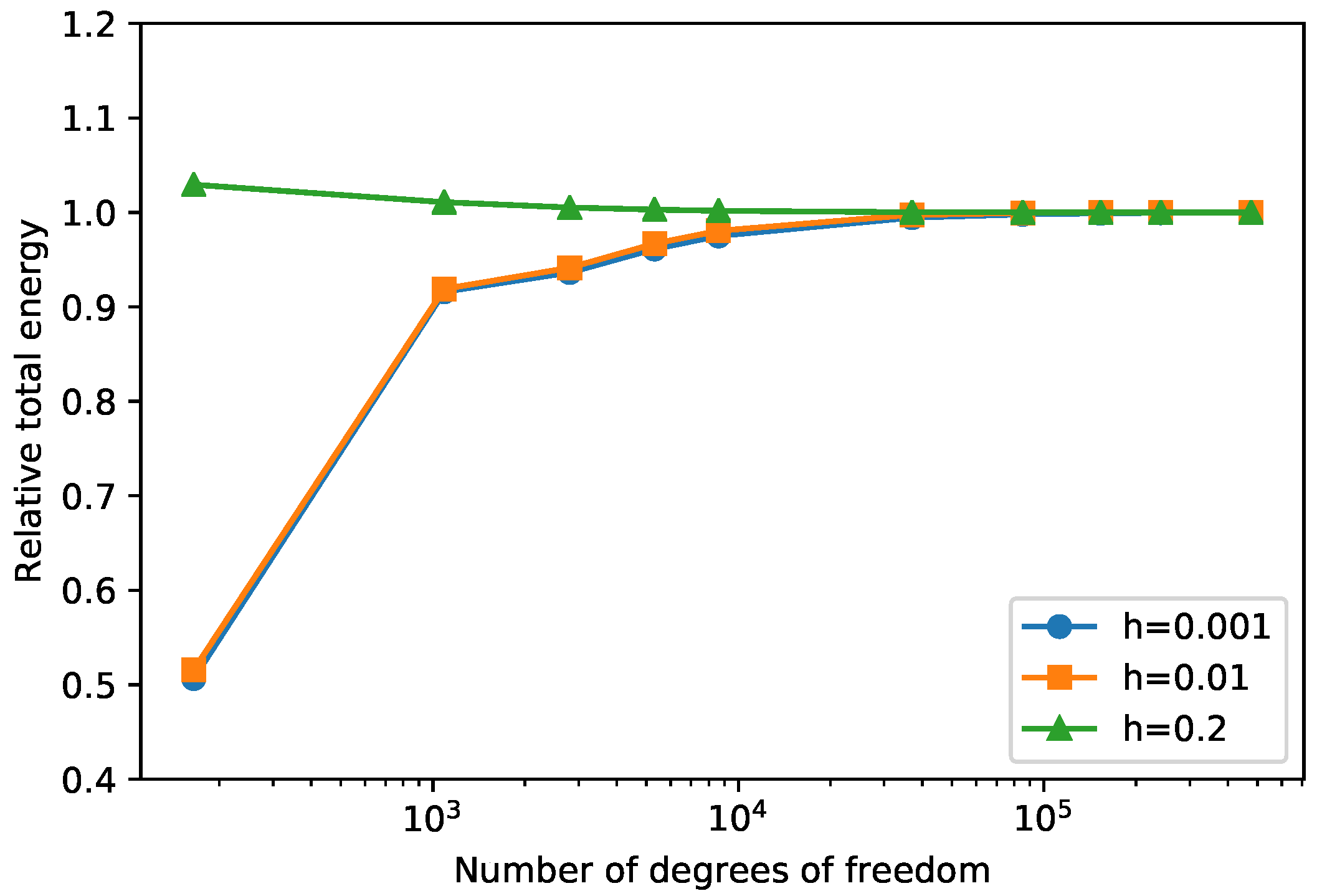
5.1. Homogeneous Laminate

We first consider a square plate of length $l=1$ m made of a homogeneous isotropic linear elastic material with $E=10$ GPa and $\nu =0.3$. We consider a thin plate case with a thickness $h=0.01$ m as well as a thick plate case with $h=0.2$ m. The boundary is assumed to be fully clamped and the plate is subjected to a uniform vertical loading of density $q=1$ MPa for the thin plate case and $q=8$ GPa for the thick plate case. Calculations are performed considering a subdivision of the plate thickness in $n=2$ layers. To compare the performance of the mixed approach with the more standard displacement-based FE interpolation, we monitor the evolution of the total elastic energy ($\frac{1}{2}a(\Sigma ,\Sigma )$ for the present mixed approach) with mesh refinement. Results are normalized with respect to the total energy of a reference solution obtained with an extremely fine mesh.

In the thick plate case ($h=0.2$ m), convergence of the total energy has been represented in Figure 3 in terms of total number of degrees of freedom. One can observe that convergence of the quadratic mixed approach $(p=2)$ is faster than the linear mixed approach ($p=1$) and the displacement approach. In particular, the total energy is already well approximated with the coarsest mesh (2 elements/side) unlike the displacement approach.

The corresponding results in the thin plate case (h = 0.01 m) have been presented in Figure 4. In this case, the quadratic mixed approach still exhibits a faster convergence than the displacement approach. However, in this case, the linear mixed approach shows an extremely slow convergence rate. This may be attributed to a lack of stability of the retained discretization choice which would require more in-depth mathematical analysis. As a result, only the mixed approach with $p=2$ will be retained in the remaining part of the paper. Finally, we can remark that, unlike the displacement approach, the quadratic mixed approach exhibits no shear-locking effect in the thin plate limit. Specific treatment such as selective reduced integration as in the displacement approach is therefore unnecessary.

Figure 5 and Figure 6 represent respectively the results of the linear mixed approach ($p=1$) and the quadratic mixed approach ($p=2$) for three different thicknesses ($h=0.001$ m, $h=0.01$ m, $h=0.2$ m). The case of linear mixed approach clearly shows shear-locking for the thin plate, while the quadratic mixed approach shows no shear-locking effect in the thin plate. Finally, we can also observe that the quadratic mixed approach, although exhibiting good convergence irrespective of the plate thickness, tends to converge from above for thick plates and from below for thinner plates. This is a confirmation that our approach is of mixed nature: it is neither a pure displacement (which would always converge from above) nor a pure static approach (which would always converge from below). We can postulate that, in the thin plate case, shear effects become negligible and our mixed approach almost satisfies exactly the equilibrium and traction continuity conditions related to the bending part, which results in a static-like convergence behavior.

Let us now compare the values of the vertical deflection $U_3$ along the plate middle line $0\le x\le 1,y=0.5$ for the thin plate $h=0.01$ m. In the displacement approach, $U_3$ is one of the primal unknowns, whereas, in the quadratic mixed approach, the deflection is computed from an $L^2$-projection of the corresponding cell Lagrange multiplier U on the space of piecewise linear Lagrange polynomials. We represent in Figure 7 the deflection of the first layer (in this case, both layers have the same deflection) on a coarse (10 elements/side) and fine (70 elements/side) mesh. It can clearly be observed that, for a coarse mesh, the projected deflection obtained from the mixed approach is more accurate than the deflection computed from the displacement approach. For a fine mesh, both solutions coincide as expected.

Finally, a similar comparison is performed regarding the horizontal membrane force $N_{11}$ in the first layer along the same middle line, see Figure 8. Regarding the displacement approach, the membrane force computed from the FE displacement solution will, a priori, be discontinuous across cells. We therefore represent, for the coarse mesh, a discontinuous version $N_{11}$ projected over a piecewise constant space as well as a “smoothed” version obtained by projecting $N_{11}$ over a continuous piecewise linear space. Such stress fields obtained from a displacement FE approach are not very accurate for a coarse mesh contrary to their counterpart obtained with a mixed approach. The projection over a continuous space even deteriorates the quality of the approximation of the discontinuous version. This is a clear advantage of mixed methods since stress fields are usually the quantities of interest used by the engineer to design mechanical systems. Obtaining more accurate estimations of stresses on a coarse mesh is thus extremely valuable.

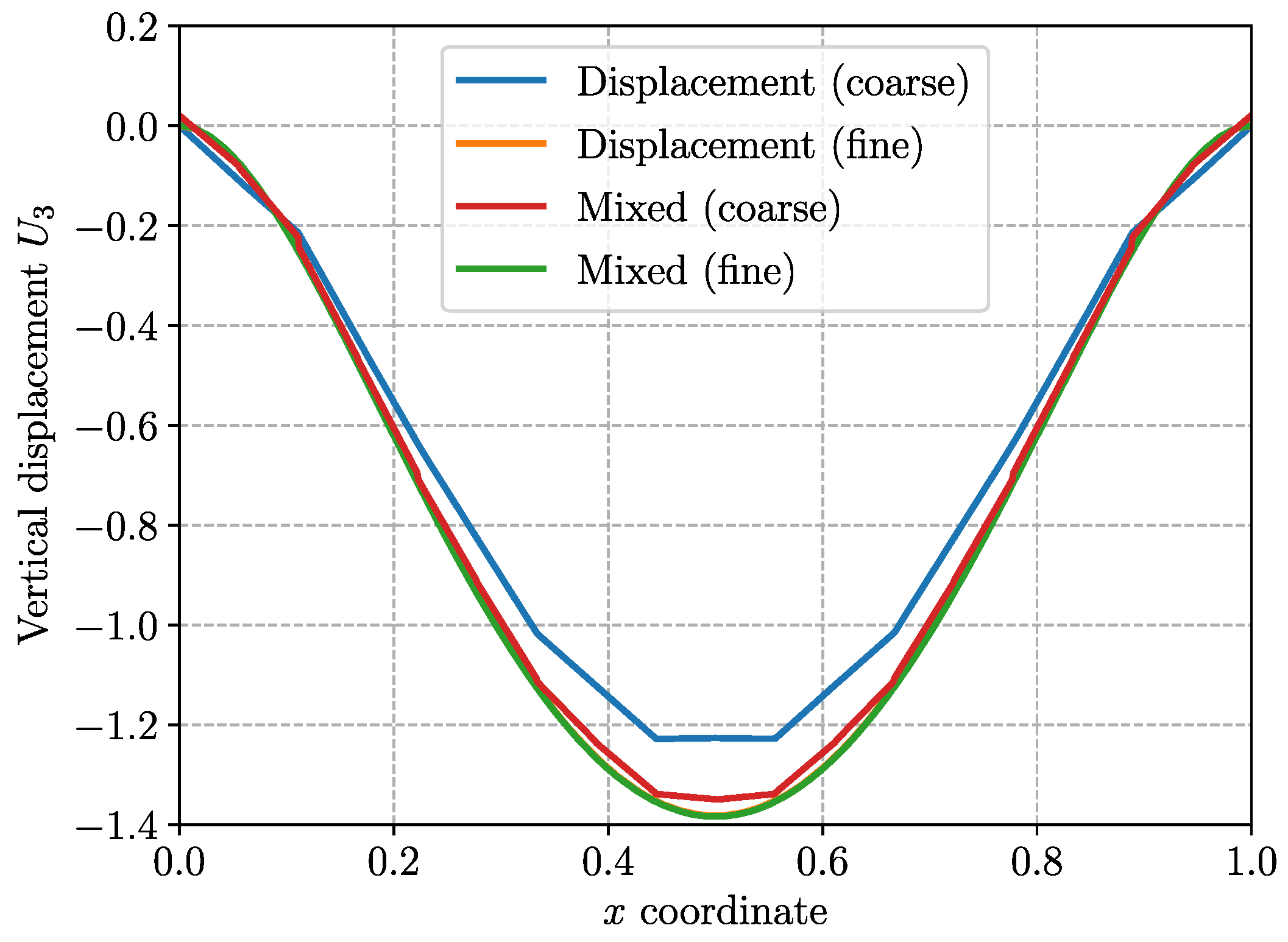
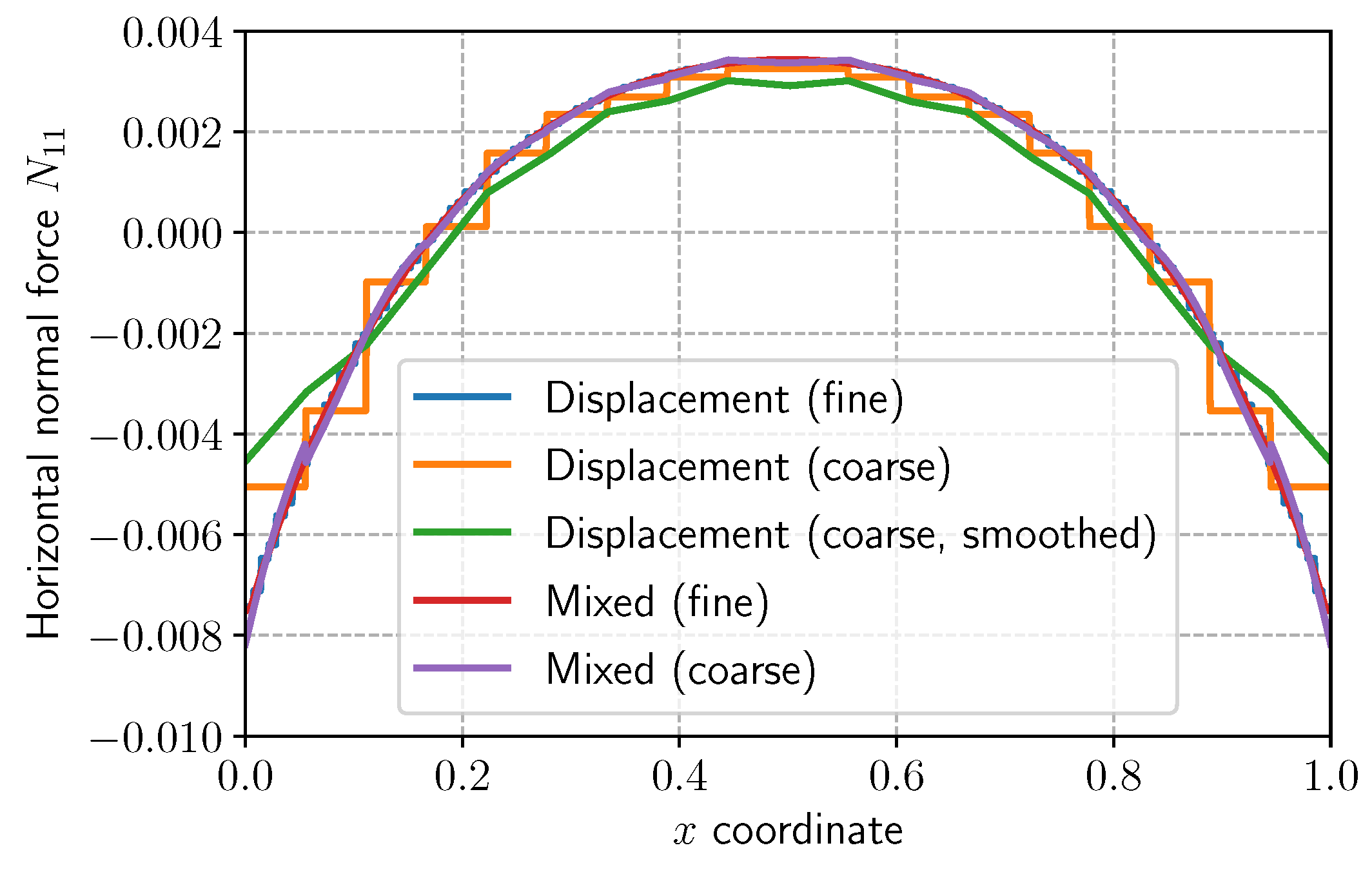
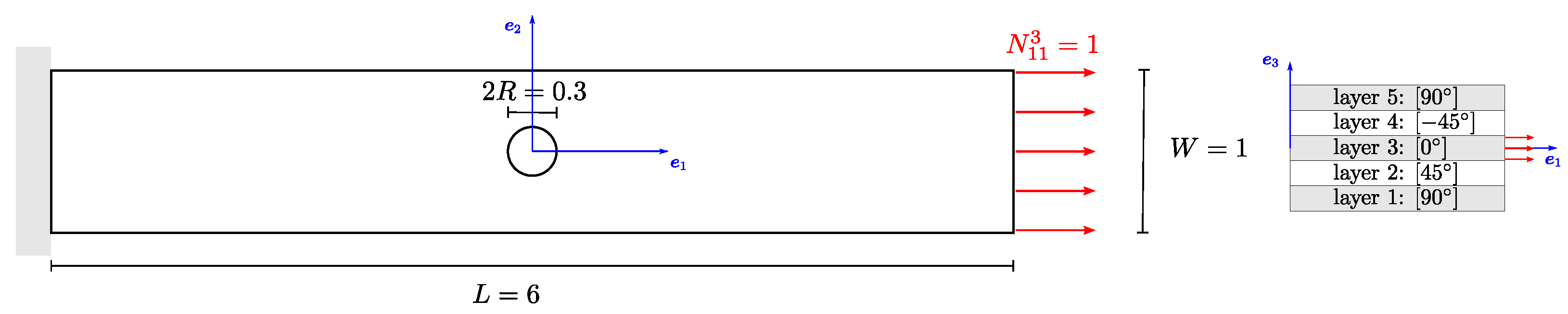
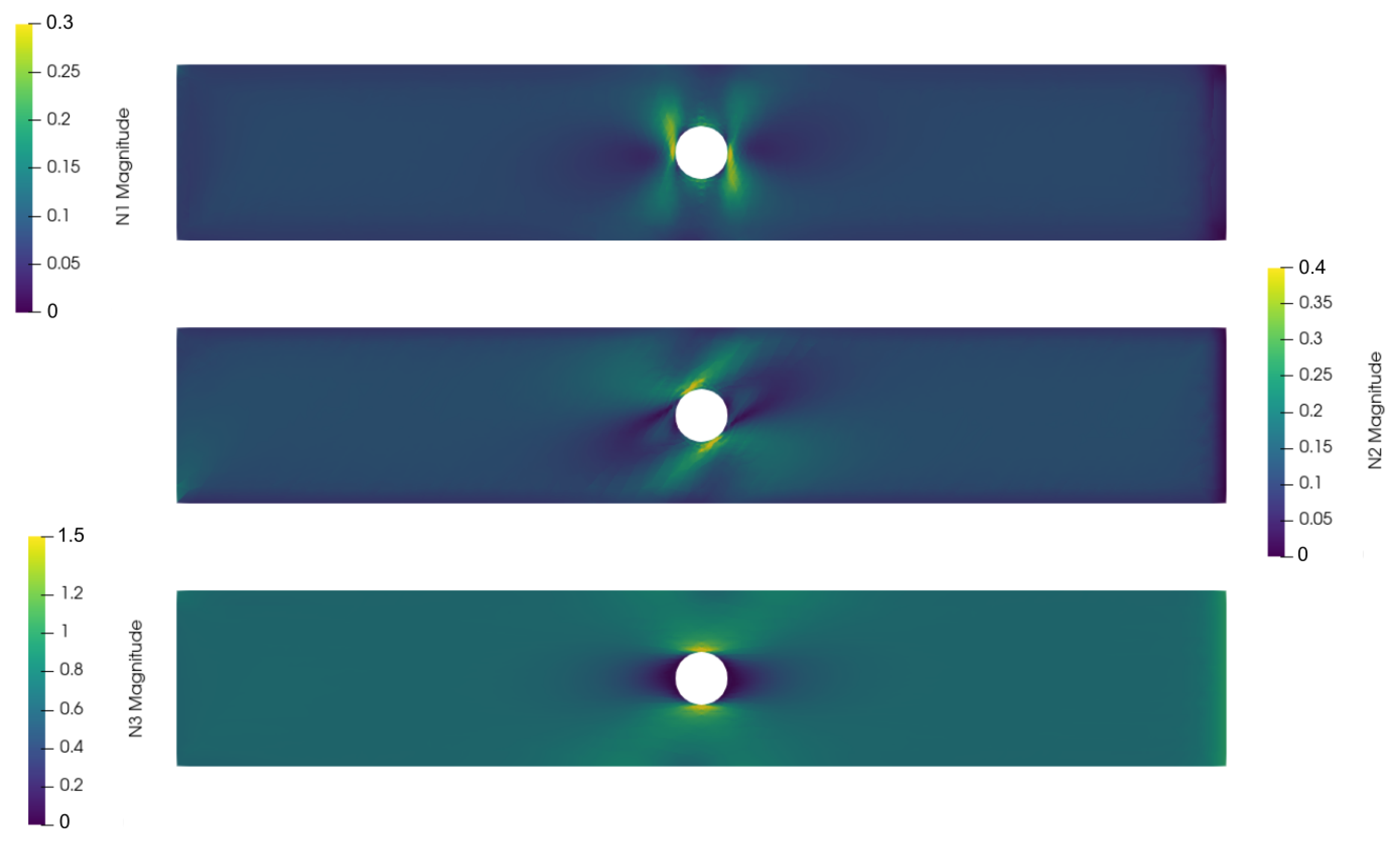
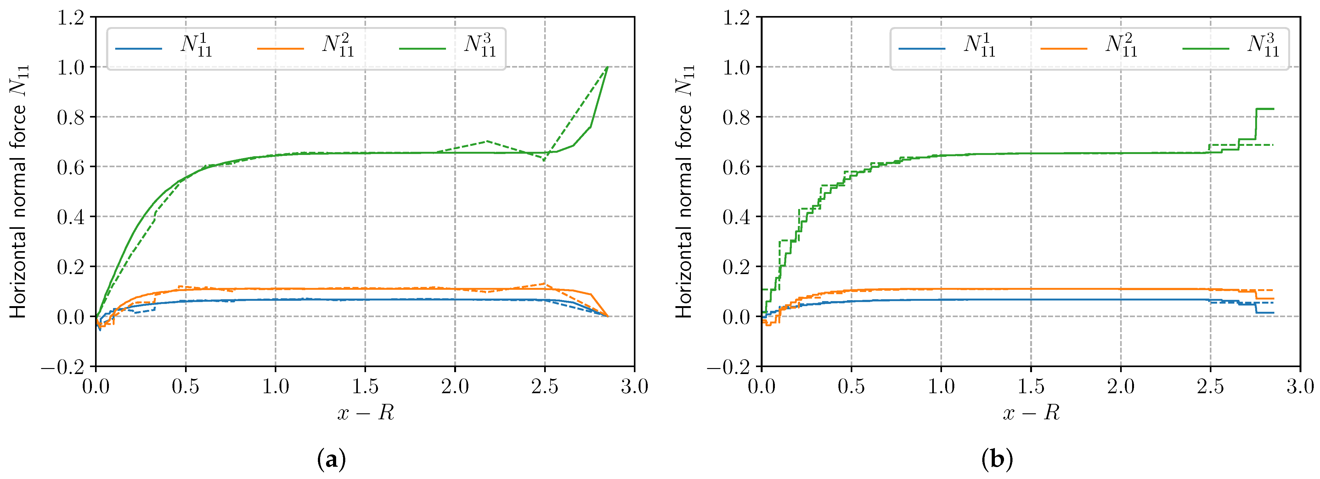
5.2. Laminate with a Circular Hole

We now investigate a rectangular plate of length $L=6$ m, width $W=1$ m and total thickness $h=0.2$ m. The plate is perforated by a circular hole of radius $R=0.15$ m in its center. The multilayered plate is made of five plies (one layer per ply) with fibers oriented at $[{90}^{\circ },{45}^{\circ },0^{\circ },-{45}^{\circ },{90}^{\circ }]$ with respect to the horizontal direction. Each ply consists of a transversely isotropic material with the following elastic properties $E_T=14.48$ GPa, $E_L=137.9$ GPa, ${\nu }_T=0.21$, ${\nu }_L=0.21$, ${\mu }_T=5.86$ GPa and ${\mu }_L=5.86$ GPa with $L\left(\mathrm{resp}. T\right)$ denoting the fiber longitudinal direction (resp. the perpendicular transverse direction). The plate is clamped on the left boundary, free on the top, bottom and on the hole boundaries. A uniform traction is applied to the 3rd layer (i.e., $N_{11}^3=1$ MPa/m) on the right boundary while the other layers remain free, as shown in Figure 9. Due to the laminate anisotropic layout, strong stress concentrations are expected at the hole boundary. Similarly, applying a traction only on the third layer will induce a boundary layer effect along which stress transfers will occur between the third layer and its adjacent ones.

As expected, Figure 10 shows that each individual layer experiences strong stress concentrations near the hole boundary. The resulting stress fields clearly illustrate the material anisotropy between the first, second and third layer.

In addition, we compare the $N_{11}$ membrane stress in the first three layers along the $y=0$, $x\ge R$ line in Figure 11 for both mixed and displacement approaches for a coarse and a fine mesh. Clearly, the mixed approach succeeds in satisfying the stress-free boundary condition on the right boundary in layers 1 and 2, even with a coarse mesh (dotted line). The edge effects near the boundary are therefore much better represented than using a displacement approach, even with a fine mesh. This feature is particularly beneficial in order to accurately predict the occurrence of delamination in composite laminates for instance.

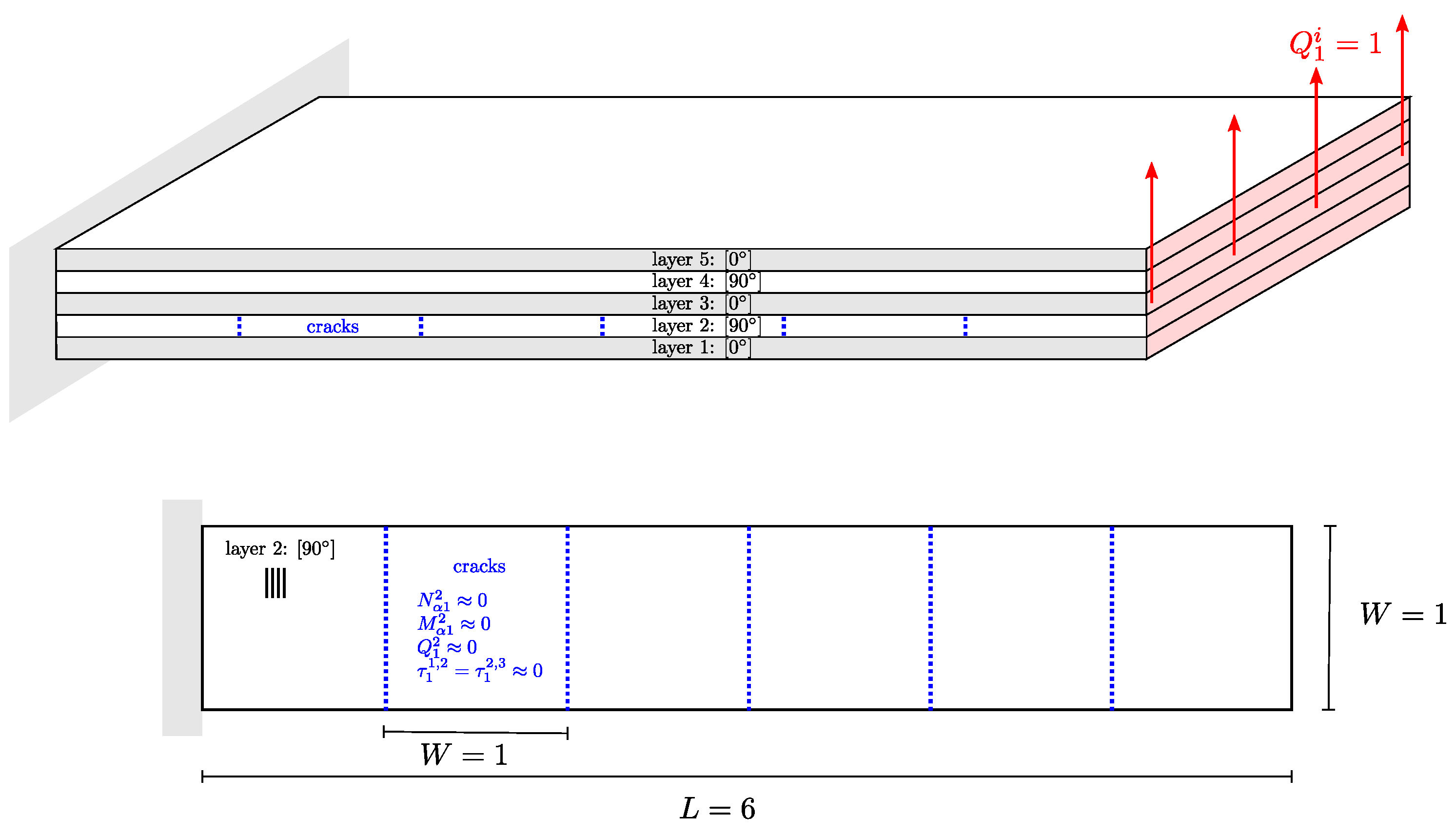
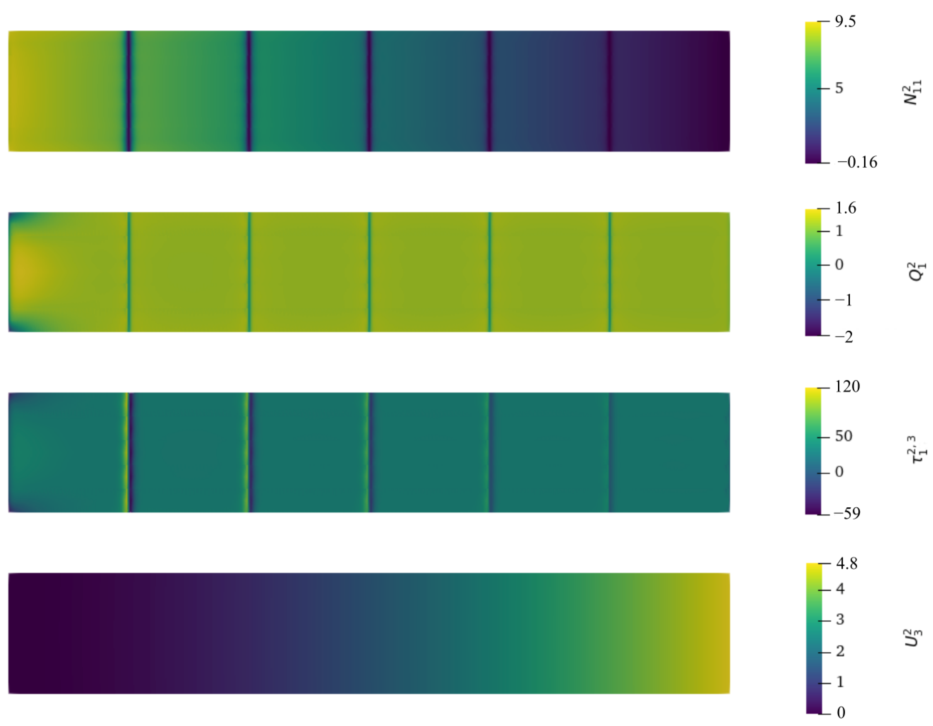
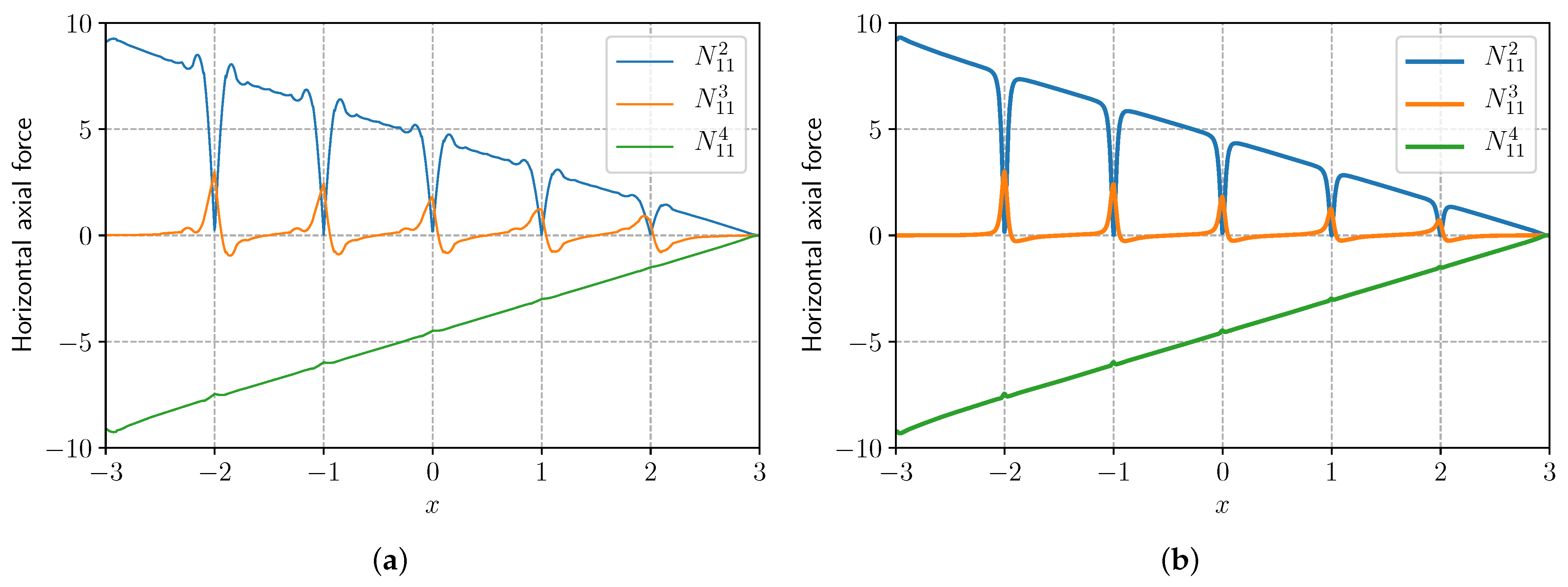
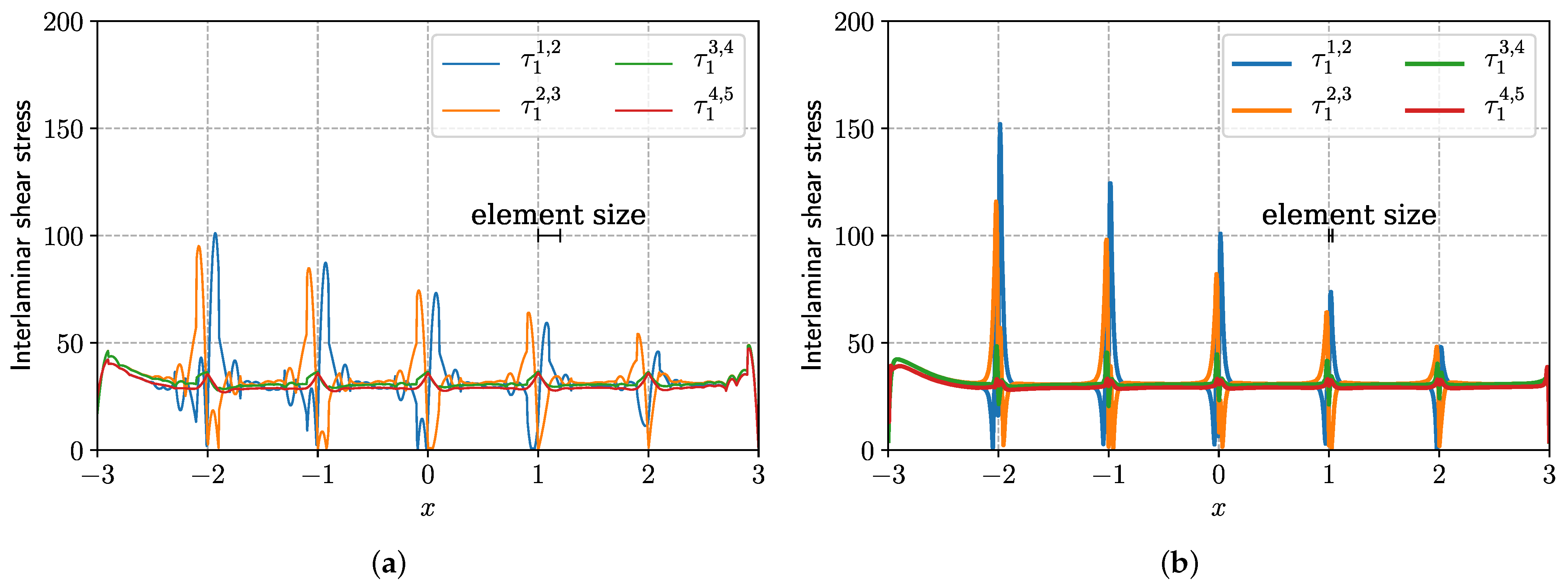
5.3. Bending of a Laminate with Multi-Cracking

The final example (Figure 12) considers a rectangular multilayered plate having the same dimensions as previously in Section 5.2 (without the circular hole). The laminate consists of five plies (one layer per ply) with fiber oriented at $[0^{\circ },{90}^{\circ },0^{\circ },{90}^{\circ },0^{\circ }]$ with respect to the horizontal direction and with the same lamination properties. The second layer is weakened by the introduction of five cracks through the ply thickness. The plate is clamped at the left border, free on its lateral sides, and a uniform vertical force is applied on the right border for all layers i.e., $Q_1^i=1$ MPa/m for $i=1,\dots ,5$.

Cracks are modeled by adding to the variational formulation (41) an additional elastic energy of the corresponding generalized tractions on the crack interface ${\Gamma }_{\mathrm{crack}}$, i.e., the bilinear form a representing the elastic energy is replaced by:

$$\begin{array}{cc}\hfill \tilde{a}(\widehat{\Sigma },\Sigma )& =a(\widehat{\Sigma },\Sigma )+a_{\mathrm{crack}}(\widehat{\Sigma },\Sigma )\hfill \end{array}$$

(42)

$$\begin{array}{cc}\hfill a_{\mathrm{crack}}(\widehat{\Sigma },\Sigma )& ={\displaystyle \frac{1}{K_{\mathrm{int}}}}{\int }_{{\Gamma }_{\mathrm{crack}}}\left({\widehat{N}}_{\alpha 1}^2{N}_{\alpha 1}^2+{\widehat{M}}_{\alpha 1}^2{M}_{\alpha 1}^2+{\widehat{Q}}_1^2{Q}_1^2+{\widehat{\tau }}_1^{1,2}{\tau }_1^{1,2}+{\widehat{\tau }}_1^{2,3}{\tau }_1^{2,3}\right)dS\hfill \end{array}$$

(43)

where the associated interface stiffness is assumed to be very small $K_{int}\ll 1$ (note that we did not pay attention to physical units in this penalized term).

Figure 13 represents the variations of the generalized stresses $N_{11}^2,Q_1^2,{\tau }_1^{2,3}$ and the vertical displacement $U_3^2$ in layer 2. As expected, the stress fields exhibit strong variations around the cracks. Indeed, these fields must vanish at the crack stress-free interface, but due to the bonding exerted by adjacent layers, stress transfers occur between the different cracked regions. The stress fields recover a value similar to what it would be without the cracks. On the contrary, the vertical displacement field remains continuous, whereas the in-plane displacement $U_1^2$ in layer 2 exhibits weak discontinuities due to the bonding of adjacent layers. As a result, a mixed approach is extremely advantageous in such situations where stresses are much more singular than displacements.

The variation of the axial stress $N_{11}$ in layers 2, 3 and 4 for a coarse mesh (5 elements between cracks) is represented in Figure 14a. When compared to the solution on a much finer mesh (Figure 14b), we notice that the strong variations near the cracks are already well captured.

Finally, the variations of the interfacial shear stress field ${\tau }_1$ at the interfaces $(1,2)$, $(2,3)$, $(3,4)$ and $(4,5)$ are represented in Figure 15. Such strong variations are harder to capture by the coarse mesh, especially when looking at the maximum values which are the quantities of interest that will drive the occurrence of interface delamination in such situations. However, we observe that coarser meshes can be used with the mixed approach to obtain an accurate estimation of such interfacial stresses.

6. Conclusions and Perspectives

In this work, we investigated an efficient discretization strategy for a stress-based layerwise plate model. A mixed finite-element discretization has been proposed as an alternative to the conventional displacement-based finite-element method. A hybridization strategy has been presented in which traction continuity is enforced explicitly through the use of an additional displacement-like Lagrange multiplier defined on the elements facets. Such a strategy offers the advantages of uncoupling many degrees of freedom. Local static condensation can be performed to yield a much smaller final system to solve. This static condensation operation on such a complex mechanical model has been made possible by recent developments in automated code-generating finite-element solvers such as Firedrake. Finally, some illustrative applications demonstrate that the proposed mixed approach is free from any shear-locking in the thin plate limit and is more accurate than a displacement approach for the same number of freedom degrees. This mixed method is therefore particularly well suited to capture strong intra-laminar and inter-laminar stress variations near free edges and cracks.

Further developments might be interesting to pursue. For instance, it is clear that such complex layerwise models are efficient and relevant in regions of strong stress variations (near cracks, holes, loading application, etc.). However, in the bulk region, i.e., far from these regions, it is known that an equivalent single layer model might be enough to describe the behavior of the laminate. An interesting perspective would then be to couple a detailed layerwise model in the previously mentioned critical regions with an ESL model in the bulk region. In this respect, the approach of [53] using the Proper Generalized Decomposition seems promising.

Finally, another natural extension of the present work is to model delamination phenomena between the different layers and simulate their propagation. Specific attention should therefore be paid to how delamination might impact the efficiency of the static condensation procedure.

References

1. Chue, C.H.; Liu, C.I. Disappearance of free-edge stress singularity in composite laminates. Compos. Struct. 2002, 56, 111–129. [Google Scholar] [CrossRef]
2. Leguillon, D. A method based on singularity theory to predict edge delamination of laminates. Int. J. Fract. 1999, 100, 105–120. [Google Scholar] [CrossRef]
3. Mittelsteda, C.; Becker, W. Asymptotic analysis of stress singularities in composite laminates by the boundary finite element method. Compos. Struct. 2005, 71, 210–219. [Google Scholar] [CrossRef]
4. Ting, T.C.T.; Chou, S.C. Edge singularities in anisotropic composites. Int. J. Solids Struct. 1981, 17, 1057–1068. [Google Scholar] [CrossRef]
5. Wang, S.S.; Choi, I. Boundary-layer effects in composite laminates Part II: Free-edge stress singularities. J. Appl. Mech. 1982, 49, 541–548. [Google Scholar] [CrossRef]
6. Cecchi, A.; Sab, K. A homogenized model for orthotropic perdiodic plates: Application to brickwork panels. Int. J. Solids Struct. 2007, 44, 6055–6079. [Google Scholar] [CrossRef] [Green Version]
7. Maenghyo, C.; Parmerter, R.R. Efficient higher order composite plate theory for general lamination configurations. AIAA J. 1993, 31, 1299–1306. [Google Scholar]
8. Lebée, A.; Sab, K. A Bending-Gradient model for thick plates. Part I: Theory. Int. J. Solids Struct. 2011, 48, 2878–2888. [Google Scholar] [CrossRef]
9. Lebée, A.; Sab, K. A Bending-Gradient model for thick plates. Part II: Closed form solutions for cylindrical bending of laminates. Int. J. Solids Struct. 2011, 48, 2889–2901. [Google Scholar] [CrossRef]
10. Lebée, A.; Sab, K. Homogenization of thick periodic plates: Application of the bending-gradient plate theory to a folded core sandwich panel. Int. J. Solids Struct. 2012, 49, 2778–2792. [Google Scholar] [CrossRef]
11. Reddy, J.N. A simple higher-order theory for laminated composite plates. J. Appl. Mech. 1984, 51, 745–752. [Google Scholar] [CrossRef]
12. Swaminathan, K.; Ragounadin, D. Analytical solutions using a higher-order refined theory for the static analysis of antisymmetric angle-ply composite and sandwich plates. Compos. Struct. 2004, 64, 405–417. [Google Scholar] [CrossRef]
13. Whitney, J.M.; Sun, C.T. A higher-order theory for extensional motion of laminates composites. J. Sound Vib. 1973, 30, 85–97. [Google Scholar] [CrossRef]
14. Vidal, P.; Polit, O. A family of sinus finite elements for the analysis of rectangular laminated beams. Compos. Struct. 2008, 84, 56–72. [Google Scholar] [CrossRef] [Green Version]
15. Vidal, P.; Polit, O. A sine finite element using a zig-zag function for the analysis of laminated composite beams. Compos. Part B Eng. 2011, 42, 1671–1682. [Google Scholar] [CrossRef] [Green Version]
16. Barbero, E.J.; Reddy, J.N. Modeling of delamination in composite laminates using a layerwise plate theory. Int. J. Solids Struct. 1991, 28, 373–388. [Google Scholar] [CrossRef]
17. Botello, S.; Oñate, E.; Canet, J.M. A layer-wise triangle for analysis of laminated composite plates and shells. Comput. Struct. 1999, 70, 635–646. [Google Scholar] [CrossRef]
18. Carrera, E. Mixed layer-wise models for multilayered plates analysis. Compos. Struct. 1998, 43, 57–70. [Google Scholar] [CrossRef]
19. Moorthy, C.M.D.; Reddy, J.N. Modeling of delamination using a layerwise element with enhanced strains. In Studies in Applied Mechanics; Elsevier: Amsterdam, The Netherlands, 1998; Volume 46, pp. 459–479. [Google Scholar]
20. Gaudenzi, P.; Barboni, R.; Mannini, A. A finite element evaluation of single-layer and multi-layer theories for the analysis of laminated plates. Comput. Struct. 1995, 30, 427–440. [Google Scholar] [CrossRef]
21. Robbins, D.H.; Reddy, J.N. Modeling of thick composites using a layerwise laminate theory. Int. J. Numer. Methods Eng. 1993, 36, 655–677. [Google Scholar] [CrossRef]
22. Carrera, E. Theories and finite elements for multilayered, anisotropic composite plates and shells. Arch. Comput. Methods Eng. 2002, 9, 87–140. [Google Scholar] [CrossRef]
23. Carrera, E. On the use of the Murakami’s zig-zag function in the modeling of layered plates and shells. Comput. Struct. 2004, 82, 541–554. [Google Scholar] [CrossRef]
24. Zhang, Y.X.; Yang, C.H. Recent developments in finite element analysis for laminated composite plates. Compos. Struct. 2009, 88, 147–157. [Google Scholar] [CrossRef]
25. Caron, J.F.; Diaz, A.D.; Carreria, R.P.; Chabot, A.; Ehrlacher, A. Multi-particle modelling for the prediction of delamination in multi-layered materials. Compos. Sci. Technol. 2006, 66, 755–765. [Google Scholar] [CrossRef]
26. Carreria, R.P.; Caron, J.F.; Diaz, A.D. Model of multilayered materials for interface stresses estimation and validation by finite element calculations. Mech. Mater. 2002, 34, 217–230. [Google Scholar] [CrossRef] [Green Version]
27. Diaz, A.D.; Caron, J.F.; Carreira, R.P. Software application for evaluating interfacial stresses in inelastic symmetrical laminates with free edges. Compos. Struct. 2002, 58, 195–208. [Google Scholar] [CrossRef]
28. Lerpiniere, A.; Caron, J.F.; Diaz, A.D.; Sab, K. The LS1 model for delamination propagation in multilayered materials at 00/θ0 interfaces: A comparison between experimental and finite elements strain energy release rates. Int. J. Solids Struct. 2014, 51, 3973–3986. [Google Scholar] [CrossRef]
29. Naciri, T.; Ehrlacher, A.; Chabot, A. Interlaminar stress analysis with a new multiparticle modelization of multilayered materials (M4). Compos. Sci. Technol. 1998, 58, 337–343. [Google Scholar] [CrossRef] [Green Version]
30. Nguyen, V.T.; Caron, J.F. A new finite element for free edges effect analysis in laminated composites. Compos. Struct. 2006, 84, 1538–1546. [Google Scholar] [CrossRef]
31. Saeedi, N.; Sab, K.; Caron, J.F. Delaminated multilayered plates under uniaxial extension. Part I: Analytical analysis using a layerwise stress approach. Int. J. Solids Struct. 2012, 49, 3711–3726. [Google Scholar] [CrossRef]
32. Saeedi, N.; Sab, K.; Caron, J.F. Delaminated multilayered plates under uniaxial extension. Part II: Very efficient layerwise mesh strategy for the prediction of delamination onset. Int. J. Solids Struct. 2012, 49, 3727–3740. [Google Scholar] [CrossRef]
33. Saeedi, N.; Sab, K.; Caron, J.F. Cylindrical bending of multilayered plates with multi-delamination via a layerwise stress approach. Compos. Struct. 2013, 95, 728–739. [Google Scholar] [CrossRef]
34. Saeedi, N.; Sab, K.; Caron, J.F. Stress analysis of long multilayered plates subjected to invariant loading: Analytical solutions by a layerwise stress model. Compos. Struct. 2013, 100, 307–322. [Google Scholar] [CrossRef]
35. Pagano, N.; Pipes, R. Interlaminar stresses in composite laminates under uniform axial extension. J. Composite Mat. 1970, 4, 538–548. [Google Scholar]
36. Baroud, R.; Sab, K.; Caron, J.F.; Kaddah, F. A statically compatible layerwise stress model for the analysis of multilayered plates. Int. J. Solids Struct. 2016, 96, 11–24. [Google Scholar] [CrossRef]
37. Nasser, H.; Chupin, O.; Piau, J.M.; Chabot, A. Mixed FEM for solving a plate type model intended for analysis of pavements with discontinuities. Road Mater. Pavement Des. 2018, 19, 496–510. [Google Scholar] [CrossRef]
38. Salha, L.; Bleyer, J.; Sab, K.; Bodgi, J. Mesh-adapted stress analysis of multilayered plates using a layerwise model. Adv. Modeling Simul. Eng. Sci. 2020, 7, 2. [Google Scholar] [CrossRef] [Green Version]
39. Logg, A.; Mardal, K.A.; Wells, G.N. Automated Solution of Differential Equations by the Finite Element Method; Springer: Berlin/Heidelberg, Germany, 2012. [Google Scholar]
40. Alnæs, M.; Blechta, J.; Hake, J.; Johansson, A.; Kehlet, B.; Logg, A.; Richardson, C.; Ring, J.; Rognes, M.E.; Wells, G.N. The FEniCS project version 1.5. Arch. Numer. Softw. 2015, 3, 9–23. [Google Scholar]
41. Fraeijs de Veubeke, B. Displacement and equilibrium models in the finite element method. In Stress Analysis; John Wiley & Sons: Hoboken, NJ, USA, 1965; Chapter 9. [Google Scholar]
42. Arnold, D.N.; Brezzi, F. Mixed and nonconforming finite element methods: Implementation, postprocessing and error estimates. ESAIM Math. Model. Numer. Anal. 1985, 19, 7–32. [Google Scholar] [CrossRef] [Green Version]
43. Cockburn, B.; Gopalakrishnan, J.; Lazarov, R. Unified hybridization of discontinuous Galerkin, mixed, and continuous Galerkin methods for second order elliptic problems. SIAM J. Numer. Anal. 2009, 47, 1319–1365. [Google Scholar] [CrossRef]
44. Brezzi, F.; Fortin, M. Mixed and Hybrid Finite Element Methods; Springer Science & Business Media: Berlin/Heidelberg, Germany, 2012; Volume 15. [Google Scholar]
45. Arnold, D.N.; Winther, R. Mixed finite elements for elasticity. Numer. Math. 2002, 92, 401–419. [Google Scholar] [CrossRef]
46. Arnold, D.; Falk, R.; Winther, R. Mixed finite element methods for linear elasticity with weakly imposed symmetry. Math. Comput. 2007, 76, 1699–1723. [Google Scholar] [CrossRef] [Green Version]
47. Gong, S.; Wu, S.; Xu, J. New hybridized mixed methods for linear elasticity and optimal multilevel solvers. Numer. Math. 2019, 141, 569–604. [Google Scholar] [CrossRef] [Green Version]
48. Gibson, T.H.; Mitchell, L.; Ham, D.A.; Cotter, C.J. Slate: Extending Firedrake’s domain-specific abstraction to hybridized solvers for geoscience and beyond. Geosci. Model Dev. 2020, 13, 735–761. [Google Scholar] [CrossRef] [Green Version]
49. Rathgeber, F.; Ham, D.A.; Mitchell, L.; Lange, M.; Luporini, F.; McRae, A.T.; Bercea, G.T.; Markall, G.R.; Kelly, P.H. Firedrake: Automating the finite element method by composing abstractions. ACM Trans. Math. Softw. 2016, 43, 1–27. [Google Scholar] [CrossRef]
50. Klöckner, A. Loo.py: Transformation-based code generation for GPUs and CPUs. In Proceedings of the ACM SIGPLAN Workshop on Libraries, Languages, and Compilers for Array Programming, Edinburgh, Scotland, 9–11 June 2014. [Google Scholar]
51. Kirby, R.C.; Mitchell, L. Solver composition across the PDE/linear algebra barrier. SIAM J. Sci. Comput. 2018, 40, C76–C98. [Google Scholar] [CrossRef]
52. Sun, T.; Mitchell, L.; Kulkarni, K.; Klöckner, A.; Ham, D.A.; Kelly, P.H. A study of vectorization for matrix-free finite element methods. arXiv 2019, arXiv:1903.08243. [Google Scholar] [CrossRef]
53. Vidal, P.; Gallimard, L.; Polit, O. Proper generalized decomposition and layer-wise approach for the modeling of composite plate structures. Int. J. Solids Struct. 2013, 50, 2239–2250. [Google Scholar] [CrossRef]
Figure 1. Notation in a layer.
Mathematics 10 01711 g001
Figure 2. (a) geometrical 2D mesh; (b) mixed approach with p = 1 ; (c) mixed approach with p = 2 .
Mathematics 10 01711 g002
Figure 3. Total energy convergence for the clamped thick plate case.
Mathematics 10 01711 g003
Figure 4. Total energy convergence for the clamped thin plate case.
Mathematics 10 01711 g004
Figure 5. Total energy convergence for the linear mixed approach ( p = 1 ) for different thicknesses.
Mathematics 10 01711 g005
Figure 6. Total energy convergence for the quadratic mixed approach ( p = 2 ) for different thicknesses.
Mathematics 10 01711 g006
Figure 7. Vertical deflection U 3 [m] for the thin plate case (both solutions in the fine mesh case are superimposed).
Mathematics 10 01711 g007
Figure 8. Horizontal membrane force N 11 [GN/m] for the thin plate case.
Mathematics 10 01711 g008
Figure 9. Laminate with circular hole under tension.
Mathematics 10 01711 g009
Figure 10. Magnitude N α β N α β [MPa/m] in layers 1, 2, and 3.
Mathematics 10 01711 g010
Figure 11. Evolution of N 11 [MPa/m] along the plate length for a coarse (dotted line) and a fine (solid line) mesh. (a) N 11 with the mixed ( p = 2 ) approach; (b) N 11 with the displacement approach.
Mathematics 10 01711 g011
Figure 12. Cracked plate problem.
Mathematics 10 01711 g012
Figure 13. Generalized stresses and vertical displacement fields in layer 2 ( N 11 2 , Q 1 2 in MPa/m, τ 1 2 , 3 in MPa, U 3 2 in m).
Mathematics 10 01711 g013
Figure 14. Axial force N 11 [MPa/m] along the plate length in layers 2, 3 and 4. (a) Coarse mesh; (b) fine mesh.
Mathematics 10 01711 g014
Figure 15. Interfacial stress τ 1 [MPa] along the plate length at all interfaces. (a) coarse mesh; (b) fine mesh.
Mathematics 10 01711 g015