Optimization of Observer Feedback Gains for Stable Sensorless IM Drives at Very Low Frequencies: A Comparative Study between GA and PSO

Abstract

Instability of an adaptive flux observer (AFO) in the regenerating mode at low frequencies is a great challenge of sensorless induction motor (SIM) drives. Zero observer feedback gains (OFGs) in the regenerating mode at low frequencies are the main reasons for moving the dominant zero of the speed estimators to the unstable region. OFGs should be appropriately selected to transfer the unstable dominant zero to the stable region. In this paper, genetic algorithm (GA) and particle swarm optimization (PSO) techniques were used to design the OFGs for a stable observer. A fair comparison of the dominant zero location between the two approaches using the optimized OFGs is presented under parameter deviation. Analytical results and the design procedure of the OFGs using the two approaches are presented under deviations of stator resistance and mutual inductance to guarantee a stable dominant zero in the regenerating mode of IM. The dominant zeros obtained by PSO had a superior location to that obtained by GA for both stator resistance and mutual inductance deviations. It was observed that one of the gains had an almost constant value over a wide range of parameter deviations. However, the value of the other gain was dependent on the deviation of machine parameters. The advantage of using PSO over GA is that the relation between the gain and parameter deviation can be represented by a deterministic and mostly linear relationship. Simulation and experimental work of the SIM drive are presented and evaluated under the optimized OFGs.

1. Introduction

Sensorless induction motor (SIM) drives have many advantages compared to sensored IM drives. Elimination of the speed sensor ensures reduction of cost, lower hardware complexity, higher reliability, better mechanical robustness, and lower maintenance requests. Sensorless control is also suitable for operating in a hostile environment [1]. Many methods have been recognized for SIM drives. They have been classified into the machine mathematical model-based methods and others that are independent of the machine model [2].

Numerous methods for SIM drives have employed the machine-model-based state observers, such as full-order observers [3,4], reduced-order observers [5], extended Kalman filters [6], nonlinear observers [7,8], and sliding mode observer [9,10].

Adaptive flux observer (AFO) ensures good estimation accuracy, robustness, and reliability at high- and medium-speed regions [11]. A large issue of machine-model-based observers is the robustness under parameters’ deviation [12] and the instability at low speeds in the regenerating mode operation [13].

An important issue is the dependence of machine-model-based observers on the machine parameters. Many research works have been reported to remedy this issue for the AFO. Methods using Routh–Hurwitz [11] and Lyapunov criteria [12] were presented to study the stability of AFO in the regenerative region due to unstable zeros. The coupling between estimation loops of rotor speed, rotor resistance, and stator resistance was described in [13,14,15]. These works analyzed the coupling effect of parameters’ variation on the stability of AFO in the low-speed region. Routh–Hurwitz criterion and root-locus were used for stability analysis of AFO to demonstrate the stable and unstable regions. To simplify the mathematical analysis and AFO complexity, the coupling effect of the three estimators were ignored in [16]. This coupling was taking into consideration in [17]. However, the AFO complexity and mathematical modelling were observed. Methods for complete stability conditions of AFO based on Routh–Hurwitz criterion [18], root-locus [19], and the linearized error dynamics [20,21,22] were derived and presented. To improve the AFO robustness to parameter deviation, design of adaptive law and parameters’ adaptation were introduced in [23]. In [24], the observer feedback gains were tuned in order to enhance the convergence rate of AFO. A comparison between the AFO and model reference adaptive system speed estimators was studied in [25] during the working in the regenerating mode. To overcome the observability obstacle of AFO around zero speed, different works were introduced. In [26], a scaling factor to design the observer feedback gains was used to alleviate the gross error influence on AFO stability. However, the observability obstacle of AFO near the zero speed without signal injection was remedied in [27] by adding a stator voltage error to the speed estimator. An auxiliary adaptive variable in AFO to modify the performance of AFO in the regenerating mode in comparison to the classic AFO was proposed in [28]. A virtual voltage injection method of AFO was described in [29] to treat the low-speed unobservable problem. However, the work in [30] employed a compensator for the estimated speed error that was produced from the virtual voltage injection method of AFO.

It is known that there are issues in speed-sensorless IM drives in the low-speed range, where speed sensor is eliminated, and rotor speed has to be estimated according to the mathematical motor model [31]. Then, uncertainty in motor parameters significantly influence the stability and precision of a speed estimation, especially in a low-speed regenerating mode [32]. Therefore, different previous works estimated the motor parameters to achieve the accuracy of speed estimation in the low-speed region [33,34]. To improve the stability of AFO for sensorless IM drives in low-speed regenerating mode, the observer feedback gains and speed adaptive scheme for AFO were designed considering the IM operating-point changes [35]. To solve the unstable issue of sensorless IM drives at low-speed operation, a virtual voltage injection method in the AFO was used to achieve a stable transfer function of the speed estimator as well as an observable rotor speed [36]. In [37], rotor speed for sensorless IM drive was estimated on the basis of AFO with a nonadaptive structure without an integrator in different of the classical adaptive law with the integrator to remedy the problem with the stabilization of the observer structure for near to zero rotor speed or in the regenerating mode of an induction machine.

In this paper, unstable regions of AFO using zero observer feedback gains were analyzed, particularly in the regenerating mode of operation due to the unstable zero of the speed estimator transfer function and the unobservable issue at zero speed. The instability of AFO increases with parameters’ deviation. To solve this unstable issue, the observer feedback gains should be properly selected. Two optimization techniques using PSO and GA are introduced. Optimal observer feedback gains under the dominant parameters’ variation using the GA and PSO optimization techniques were designed. The dominant zero location of AFO using both zero observer feedback gains and optimized observer feedback gains was analyzed and compared. To solve the issue of offline optimization techniques for real-time implementation, a curve fitting to extract a formula for the observer feedback gains was used. A significant improvement of the AFO under the proposed OFGs was observed. Detailed simulation and experimental verification confirmed the stability improvement, particularly at low speeds in the regenerating mode.

This paper can be organized into the following sections: Section 2 presents models of the IM, AFO, and a speed estimator. Derivation in stability conditions of AFO is analyzed in Section 3. In Section 4, OFG optimization using GA and PSO approaches is presented. Special attention is paid for the comparison between the PSO and GA for designing the OFGs, which give the optimal dominant zero location for stable AFO. Section 5 describes detailed simulation and practical tests. This paper ends with a short conclusion, as given in Section 6.

2. Mathematical Models

2.1. Induction Motor Model

The IM dynamic dq model is introduced in the stationary reference frame by (1).

$$\frac{d}{dt}\left[\begin{array}{c}{i}_{ds}^s\\ i_{qs}^s\\ {\mathsf{\lambda }}_{dr}^s\\ {\mathsf{\lambda }}_{qr}^s\end{array}\right]=\left[\begin{array}{cccc}a& 0& c& d{\mathsf{\omega }}_r\\ 0& a& -d{\mathsf{\omega }}_r& c\\ g& 0& -f& -{\mathsf{\omega }}_r\\ 0& g& {\mathsf{\omega }}_r& -f\end{array}\right]\left[\begin{array}{c}{i}_{ds}^s\\ i_{qs}^s\\ {\mathsf{\lambda }}_{dr}^s\\ {\mathsf{\lambda }}_{qr}^s\end{array}\right]+b\left[\begin{array}{c}{v}_{ds}^s\\ v_{qs}^s\\ 0\\ 0\end{array}\right]$$

(1)

where

$$\begin{array}{l}a=-\left(\frac{R_s}{\mathsf{\sigma }{L}_s}+\frac{L_m^2}{\mathsf{\sigma }{L}_s{T}_r{L}_r}\right), c=\frac{1}{\mathsf{\epsilon }{T}_r}, d=\frac{1}{\mathsf{\epsilon }}, g=\frac{L_m}{T_r}\\ \mathsf{\epsilon }=\frac{\mathsf{\sigma }{L}_s{L}_r}{L_m}, b=\frac{1}{\mathsf{\sigma }{L}_s}, \mathsf{\sigma }=1-\frac{L_m^2}{L_s{L}_r}, T_r=\frac{L_r}{R_r}, f=\frac{1}{T_r}\end{array}$$

$v_{ds}^s \mathrm{and} v_{qs}^s$ are dq stator voltages; $i_{ds}^s \mathrm{and} i_{qs}^s$ are dq stator currents; $i_{dr}^s \mathrm{and} i_{qr}^s$ are the dq currents of the rotor; ${\mathsf{\lambda }}_{ds}^s \mathrm{and} {\mathsf{\lambda }}_{qs}^s$ are the dq flux linkages of the stator; ${\mathsf{\lambda }}_{dr}^s \mathrm{and} {\mathsf{\lambda }}_{qr}^s$ are the dq flux linkages of the rotor; R_r and R_s are the rotor and stator resistances; L_s, L_m, and L_r are the stator inductance, magnetizing inductance, and the rotor inductance, respectively; and ω_r is the rotor speed.

2.2. Adaptive Flux Observer Model

On the basis of (1), AFO is expressed in the stationary reference frame using (2):

$$\frac{d}{dt}\left[\begin{array}{c}{\widehat{i}}_{ds}^s\\ {\widehat{i}}_{qs}^s\\ {\widehat{\mathsf{\lambda }}}_{dr}^s\\ {\widehat{\mathsf{\lambda }}}_{qr}^s\end{array}\right]=\left[\begin{array}{cccc}a& 0& c& d{\widehat{\mathsf{\omega }}}_r\\ 0& a& -d{\widehat{\mathsf{\omega }}}_r& c\\ g& 0& -f& -{\widehat{\mathsf{\omega }}}_r\\ 0& g& {\widehat{\mathsf{\omega }}}_r& -f\end{array}\right]\left[\begin{array}{c}{\widehat{i}}_{ds}^s\\ {\widehat{i}}_{qs}^s\\ {\widehat{\mathsf{\lambda }}}_{dr}^s\\ {\widehat{\mathsf{\lambda }}}_{qr}^s\end{array}\right]+b\left[\begin{array}{c}{v}_{ds}^s\\ v_{qs}^s\\ 0\\ 0\end{array}\right]+\left[\begin{array}{c}{K}_1{e}_{id}\\ K_2{e}_{iq}\\ 0\\ 0\end{array}\right]$$

(2)

where K₁ and K₂ are the current observer gains, $e_{id}={\widehat{i}}_{ds}^s-i_{ds}^s$ and $e_{iq}={\widehat{i}}_{qs}^s-i_{qs}^s$. From (1) and (2), the current and flux errors can be obtained using (3)

$$\frac{d}{dt}\left[\begin{array}{c}{e}_{id}\\ e_{iq}\\ e_{\mathsf{\lambda }d}\\ e_{\mathsf{\lambda }q}\end{array}\right]=\left[\begin{array}{cccc}a+K_1& 0& c& d{\mathsf{\omega }}_r\\ 0& a+K_2& -d{\widehat{\mathsf{\omega }}}_r& c\\ g& 0& -f& -{\widehat{\mathsf{\omega }}}_r\\ 0& g& {\widehat{\mathsf{\omega }}}_r& -f\end{array}\right]\left[\begin{array}{c}{e}_{id}\\ e_{iq}\\ e_{\mathsf{\lambda }d}\\ e_{\mathsf{\lambda }q}\end{array}\right]+\Delta {\mathsf{\omega }}_r\left[\begin{array}{c}d{\widehat{\mathsf{\lambda }}}_{qr}^s\\ -d{\widehat{\mathsf{\lambda }}}_{dr}^s\\ -{\widehat{\mathsf{\lambda }}}_{qr}^s\\ {\widehat{\mathsf{\lambda }}}_{dr}^s\end{array}\right]$$

(3)

where $\mathsf{\Delta }{\mathsf{\omega }}_r={\mathsf{\omega }}_r-{\widehat{\mathsf{\omega }}}_r$, $e_{\mathsf{\lambda }d}={\widehat{\mathsf{\lambda }}}_{dr}^s-{\mathsf{\lambda }}_{dr}^s$, $e_{\mathsf{\lambda }q}={\widehat{\mathsf{\lambda }}}_{qr}^s-{\mathsf{\lambda }}_{qr}^s$.

The estimators of rotor speed and stator resistance can be expressed using (4) and (5) [5].

$${\widehat{\mathsf{\omega }}}_r=(K_{P\mathsf{\omega }}+K_{I\mathsf{\omega }}{\displaystyle \int dt){\overrightarrow{e}}_{{}^i}^T}J{\widehat{\overrightarrow{\mathsf{\lambda }}}}_r^s$$

(4)

$${\widehat{R}}_s=\left(K_{PR}+K_{IR}{\displaystyle \int dt}\right){\overrightarrow{e}}_{{}^i}^T{\widehat{\overrightarrow{i}}}_s^s$$

(5)

The block diagram of the indirect field-oriented control (IFOC) of SIM is shown in Figure 1.

2.3. Speed Observer Analysis

For stability analysis of AFO in the regenerating mode at low speeds, a speed estimator transfer function can be obtained by assuming the speed as a variable parameter. The relationship between the errors in rotor speed and stator current is obtained by (6) and (7). More derivation details can be found in [5,6,7,8].

$$p{\overrightarrow{e}}_i=\left(A_{11}-K\right){\overrightarrow{e}}_i+A_{12}{\overrightarrow{e}}_{\mathsf{\lambda }}+\Delta A_{12}{\widehat{\overrightarrow{\mathsf{\lambda }}}}_r^s+\Delta A_{11}{\widehat{\overrightarrow{i}}}_s^s$$

(6)

$$p{\overrightarrow{e}}_{\mathsf{\lambda }}=A_{21}{\overrightarrow{e}}_i+A_{22}{\overrightarrow{e}}_{\mathsf{\lambda }}+\Delta A_{22}{\widehat{\overrightarrow{\mathsf{\lambda }}}}_r^s$$

(7)

where

$$\begin{gathered} {\overrightarrow{e}}_{\mathsf{\lambda }}={\widehat{\overrightarrow{\mathsf{\lambda }}}}_r^s-{\overrightarrow{\mathsf{\lambda }}}_r^s, \\ \Delta A=\widehat{A}-A=\left[\begin{array}{cc}\Delta A_{11}& \Delta A_{12}\\ \Delta A_{21}& \Delta A_{22}\end{array}\right] \end{gathered}$$

Considering the speed as the only variable parameter, the error matrix ΔA can be derived as

$$\Delta A_{11}=0, \Delta A_{12}=\frac{\Delta {\mathsf{\omega }}_{r}J}{\mathsf{\epsilon }}, \Delta A_{21}=0, \Delta A_{22}=-\Delta {\mathsf{\omega }}_{r}J$$

Applying Laplace transform to (6) and (7) gives

$$\left[sI-\left(A_{11}-K\right)\right]{\overrightarrow{e}}_i=A_{12}{\overrightarrow{e}}_{\mathsf{\lambda }}+\Delta A_{12}{\widehat{\overrightarrow{\mathsf{\lambda }}}}_r^s+\Delta A_{11}{\widehat{\overrightarrow{i}}}_s^s$$

(8)

$$\left[sI-A_{22}\right]{\overrightarrow{e}}_{\mathsf{\lambda }}=A_{21}{\overrightarrow{e}}_i+\Delta A_{22}{\widehat{\overrightarrow{\mathsf{\lambda }}}}_r^s$$

(9)

The stator current error can be expressed using a speed error as [5]

$${\overrightarrow{e}}_{\mathsf{\omega }}=G_{\mathsf{\omega }}(s)\cdot J{\widehat{\overrightarrow{\mathsf{\lambda }}}}_r^s\Delta {\mathsf{\omega }}_r$$

(10)

where

$$G_{\mathsf{\omega }}(s)=\frac{s}{\mathsf{\epsilon }}{\left[s^{2}I+s\left(a_{1}I+a_{2}J\right)+\left(a_{3}I+a_{4}J\right)\right]}^{-1}$$

(11)

$$\begin{gathered} a_1=\left(\frac{R_s}{\mathsf{\sigma }{L}_s}+\frac{L_m^2}{\mathsf{\sigma }{L}_s{T}_r{L}_r}+\frac{1}{T_r}+K_1\right) \\ {a}_2=\left(K_2-{\mathsf{\omega }}_r\right) \\ {a}_3=\left[\frac{1}{T_r}\left(\frac{R_s}{\mathsf{\sigma }{L}_s}+\frac{L_m^2}{\mathsf{\sigma }{L}_s{T}_r{L}_r}-\frac{L_m}{\mathsf{\epsilon }{T}_r}+K_1\right)+K_2{\mathsf{\omega }}_r\right] \\ {a}_4=\left[\frac{K_2}{T_r}-{\mathsf{\omega }}_r\left(\frac{R_s}{\mathsf{\sigma }{L}_s}+\frac{L_m^2}{\mathsf{\sigma }{L}_s{T}_r{L}_r}-\frac{L_m}{\mathsf{\epsilon }{T}_r}+K_1\right)\right] \end{gathered}$$

Then, Equation (10) gives

$$e_{1q}=\left|{\widehat{\mathsf{\lambda }}}_r^s\right|{G^{\prime }}_{\mathsf{\omega }22}(s)\Delta {\mathsf{\omega }}_r$$

(12)

The TF of ${G^{\prime }}_{\mathsf{\omega }22}(s)$ can be expressed by (13). It is derived to plot a root locus for poles/zeros allocation.

$${G^{\prime }}_{\mathsf{\omega }22}(s)=\frac{s^3+a_1{s}^2+\left({\mathsf{\omega }}_o^2+a_3\right)s+{\mathsf{\omega }}_o^2{a}_1+{\mathsf{\omega }}_o{a}_4}{\mathsf{\epsilon }\left[{\left(s^2+a_{1}s-{\mathsf{\omega }}_o^2-{\mathsf{\omega }}_o{a}_2+a_3\right)}^2+{\left(\left(2{\mathsf{\omega }}_o+a_2\right)s+{\mathsf{\omega }}_o{a}_1+a_4\right)}^2\right]}$$

(13)

where ω_o is the rotor flux frequency.

3. Derivation of AFO Stability Conditions

The zeros of $G_{\mathsf{\omega }22}^{\prime }\left(s\right)$ must be located at the left-half s-plane only; otherwise, the dominant poles will be unstable.

The Routh–Hurwitz criterion was used to obtain the conditions that maintain the roots of the numerator of $G_{\mathsf{\omega }22}^{\prime }\left(s\right)$ in the stable region. The following conditions were obtained:

$${\mathsf{\omega }}_o\left({\mathsf{\omega }}_o-{\mathsf{\omega }}_{cr}\right)>0$$

(14)

$$a_1>0$$

(15)

$$a_1{a}_3-a_4{\mathsf{\omega }}_o>0$$

(16)

where ${\mathsf{\omega }}_{cr}=-\frac{a_4}{a_1}$ is the critical frequency.

From (14), the condition of stable zeros is guaranteed if the critical frequency becomes less than the operating frequency ${\mathsf{\omega }}_{cr}<{\mathsf{\omega }}_o$. Otherwise, the AFO becomes unstable.

Condition (15) is satisfied only if the observer feedback gain K₁ = 0 as a design restriction.

Finally, unstable complex conjugate zeros of $G_{\mathsf{\omega }22}^{\prime }\left(s\right)$ occurs if the condition (16) is violated; consequently, the dominant corresponding poles of $G_{\mathsf{\omega }22}^{\prime }\left(s\right)$ will move toward the unstable zeros.

Setting the feedback gains K₁ and K₂ to zero in the constants a₁, a₃, and a₄, the condition (16) becomes

$$-{\mathsf{\omega }}_o\cdot {\mathsf{\omega }}_r<\frac{1}{T_r}\left(\frac{R_s}{\mathsf{\sigma }{L}_s}+\frac{L_m^2}{\mathsf{\sigma }{L}_s{T}_r{L}_r}+\frac{1}{T_r}\right)$$

(17)

Condition (16) may be violated only under (${\mathsf{\omega }}_o\cdot {\mathsf{\omega }}_r<0$). This occurs in the plugging mode when the slip frequency is larger than ${\mathsf{\omega }}_o$ & ${\mathsf{\omega }}_r$. Practically, these unstable zeros can hardly occur in normal operation since the slip frequency is only about (3–5) % of the rated frequency.

From the presented analysis, it can be concluded that, condition (16) is the most severe stability restriction for AFO. To satisfy this condition, the working frequency should exceed the critical frequency.

At zero feedback gains (K₁ = K₂ = 0), the critical frequency is dependent on the speed and can be computed as

$${\mathsf{\omega }}_{cr}=\frac{{\mathsf{\omega }}_r}{1+\left(\frac{\mathsf{\sigma }{L}_s}{R_s{T}_r}+\frac{L_m^2}{R_s{T}_r{L}_r}\right)}$$

(18)

On the basis of (18), it is clear that ${\mathsf{\omega }}_{cr}<{\mathsf{\omega }}_r$. Therefore, two cases can be considered:

Case 1:

${\mathsf{\omega }}_r<{\mathsf{\omega }}_o$(motoring mode). Condition (14) with ${\mathsf{\omega }}_{cr}<{\mathsf{\omega }}_o$is ensured.

Case 2:

${\mathsf{\omega }}_r>{\mathsf{\omega }}_o$(regenerating mode) with negative loads. From (14), it can be derived that the unstable issue arises only when working under the condition of ${\mathsf{\omega }}_o<{\mathsf{\omega }}_{cr}<{\mathsf{\omega }}_r$.

This occurs under negative loads during the regenerating mode. The design of OFGs (K₁ and K₂) in the regenerating mode is considered the main stability issue for AFO [25,26,27,28,29,30]. Root locus plot is used to study the stability of AFO using (13). At zero OFGs (K₁ = K₂ = 0), the theoretical analysis of dominant zero locations in motoring and regenerating modes are given in Figure 2 and Figure 3, respectively. It is observed that the AFO is a stable in the motoring mode with zero OFGs as shown in Figure 2. However, instability issue is observed in the regenerating mode with zero OFGs as shown in Figure 3 due to the unstable zero of the speed estimator (13).

To deal with this obstacle, the OFGs should be appropriately selected. Previous works have designed the OFGs by different mathematical algorithms. These works guarantee the stability and ensure a good dynamic performance. However, the fixed OFGs cannot achieve the desired performance under different operating conditions, particularly parameter mismatch. Therefore, the motivation of this paper is to design the OFGs to guarantee a stable AFO, particularly at low speeds in the regenerating mode. These OFGs are tuned under parameter mismatch to ensure a good dynamic performance. Two optimization approaches using GA and PSO techniques are employed for this purpose. The OFGs are tuned under parameter mismatch.

4. Optimization of OFGs Using GA and PSO

The OFGs are optimized under parameter mismatch to enhance the dynamic performance of the system to guarantee a stable AFO, particularly at low speeds in the regenerating mode. Two optimization algorithms (GA and PSO) are employed and compared for this purpose.

4.1. Genetic Algorithm

GA is a powerful modern optimization algorithm that searches for a global optimal solution to complicated optimization problems. It is inspired by natural selection and natural genetics. It is started with a random population of guesses that will spread throughout the search space. Selection, crossover, and mutation are applied iteratively to force the algorithm towards the optimal solution. More details on the GA model can be found in [38].

4.2. Particle Swarm Optimization Technique

PSO is a population-based optimization technique inspired by social behavior of bird flocking. Particles fly around in the search space where each particle updates its position according to self-experience and the neighbor particles experience. In the solution swarm, particles are flown through the search space by following the current optimum particle. Each particle keeps track of its own best solution that it has achieved so far (pbest). The best value obtained so far by any particle in the swarm is known as the global best (gbest). PSO modelling and details can be found in [39].

The OFGs are optimized by GA and PSO under deviations of stator resistance and mutual inductance to guarantee a stable dominant zero in the regenerating mode. The dominant zeros obtained by PSO have a superior location than that obtained by GA for both stator resistance and mutual inductance deviations, as shown in Figure 4.

The optimal adaptation of OFGs (K₁ and K₂) are shown in Figure 5. It is shown that the value of K₂ has almost constant value over a wide range of deviations either in resistance or mutual inductance. Therefore, K₂ is independent on the parameters’ uncertainties, and it will be kept constant at (−0.6356). However, the value of K₁ is dependent on the deviation of machine parameters (R_s, L_m).

A very useful advantage of using PSO over GA is that the relation between K₁ and resistance or reactance deviations can be represented by a deterministic and mostly linear relationship. This relationship can be extracted from designing gain K₁ over a wide range of resistance and reactance deviations, as shown in Figure 6.

To extract a formula for gain K₁ as a function of deviation in stator resistance and mutual inductance (ΔR_s, ΔL_m), the 3D relationship in Figure 6 was analyzed considering the following cases:

Base Case:

The gain K₁ is designed at each operating point of (ΔR_s, ΔL_m) over a wide range of variations. This case is considered the reference used to measure the degree of accuracy for the extracted relationships in other cases.

Case 1:

The gain K₁ is designed considering the deviation in resistance ΔR_s, while the deviation in the mutual inductance is considered constant (i.e., ΔL_m = 0) and its effect is neglected. From the linear relationship between gain K₁ and ΔR_s, as shown in Figure 6, the following formula can be deduced:

$$K_1=a_1·\Delta R_s+a_2$$

Case 2:

The gain K₁ is designed considering the deviation in resistance ΔR_s as well as the deviation in reactance ΔL_m. The linear relationship between K₁ and ΔR_s can be extracted from Figure 7, as in the following formula:

$$F_1\left(\Delta R_s\right)=b_1·\Delta R_s+b_2$$

The superimposed effect of ΔL_m on the observer feedback gain K₁ can be extracted linearly from Figure 7, as in the following formula:

$$\begin{gathered} F_2\left(\Delta L_m\right)=b_3·\Delta L_m·\left(b_4·\Delta R+b_5\right) \\ {K}_1=F_1\left(\Delta R_s\right)+F_2\left(\Delta L_m\right) \end{gathered}$$

Case 3:

The gain K₁ is designed considering a linear deviation in resistance ΔR_s while considering a quadratic deviation in reactance ΔL_m as in the following formula:

$$\begin{gathered} K_1=C_1·{(\Delta L_m)}^2+C_2·\Delta L_m+C_3 \\ {C}_1=c_1·\Delta R_s+c_2 \\ {C}_2=c_3·\Delta R_s+c_4 \\ {C}_3=c_5·\Delta R_s+c_6 \end{gathered}$$

In the extracted formulas in all cases, the constants are deduced from the curve fitting, as given in

Table 1. Extracted formulas and associated constants.

Formula/Constant		Curve Fitting Value
$K_1=a_1·\Delta R_s+a_2$	a1	0.116270
	a2	11.633000
$K_1=F_1(\Delta R_s)+F_2(\Delta L_m)$	b1	0.116600
	b2	11.662000
	b3	−0.025000
	b4	0.007938
	b5	0.696600
$K_1=C_1·{(\Delta L_m)}^2+C_2·\Delta L_m+C_3$	c1	1.29830 × 10−6
	c2	1.13030 × 10−4
	c3	−1.97280 × 10−4
	c4	−0.017315
	c5	0.116080
	c6	11.617000

.

Figure 8 shows a comparison between the error measures for the different formulas in the proposed design cases of the gain K₁. Case 3 involving the quadratic representation gives superior error measures compared to the other two design methods.

5. Simulation and Experimental Results

5.1. Performance at Very Low Speed during Motoring Mode

Simulation and practical tests displaying the behavior of SIM drive at very low speeds are presented in Figure 9 and Figure 10, respectively. The rated values and parameters of the IM are given in Appendix A (

Table A1. The rated values and parameters of the IM.

Rated output power	5.5 kW	Stator self-inductance	57.3 mH
Rated voltage	186 V	Rotor self-inductance	57.3 mH
Rated frequency	50 Hz	Mutual inductance	56.43 mH
No. of pole pairs	2	Stator resistance	0.294 Ω
		Rotor resistance	0.14325 Ω

). A speed reference of 0.04 p.u (6.28 rad/s) was applied at T_L = 0. Then, T_L = +7 N.m at t = 2 s was applied. The first subplot displays the actual (black color) and estimated (red color) speeds in p.u. The second subplot demonstrates the iqs current component in Ampere. The third subplot presents the d-q rotor fluxes in p.u. It is noted that the estimated speed properly tracked the actual speed. This agrees with the theoretical analysis that the operation of SIM drive has no stability issue at very low speeds in the motoring mode.

5.2. Working at Very Low Speed during Regenerating Mode

To confirm the theoretical analysis of stable and unstable operation of SIM drive at very low speed during regenerating mode, we present the simulation and experimental tests in Figure 11 and Figure 12, respectively. In the simulation results, the speed reference of 0.08 p.u (12.56 rad/s) was applied at no-load torque (T_L = 0), and the negative rated load torque change of T_L = −7 N.m was applied at t = 2 s. In the experimental results, the speed reference of 0.08 p.u (12.56 rad/s) was applied at no-load torque (T_L = 0), and the negative rated load torque change of T_L= −7 N.m was applied at t = 2.2 s. It was observed that the estimated speed diverged from the actual speed. The current iqs was distorted and deviated of the actual value. The dq-rotor fluxes diverged from the rated values. Then, the speed SIM drive was unstable with zero OFGs (K₁ = K₂ = 0). This agrees with the theoretical analysis that the operation of SIM drive has a stability issue at very low speeds in the regenerating mode.

Identical simulation and experimental results are presented using the proposed OFGs in Figure 13 and Figure 14, respectively. As is obvious, the estimated speed properly tracked the actual speed. In the regenerating mode of SIM drive, the performance at very low speeds was stable with the proposed OFGs.

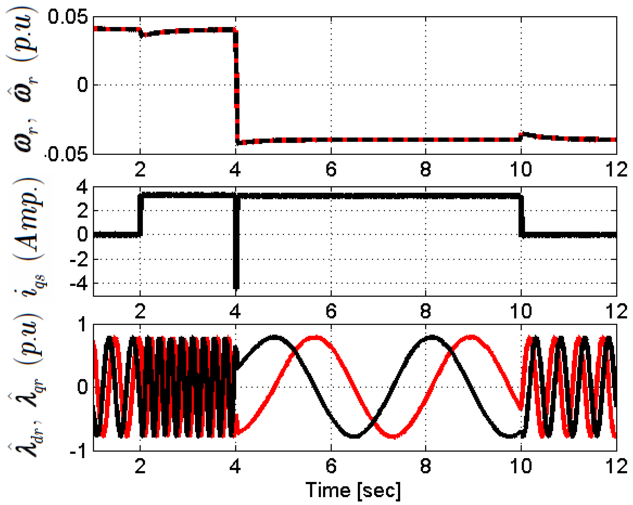
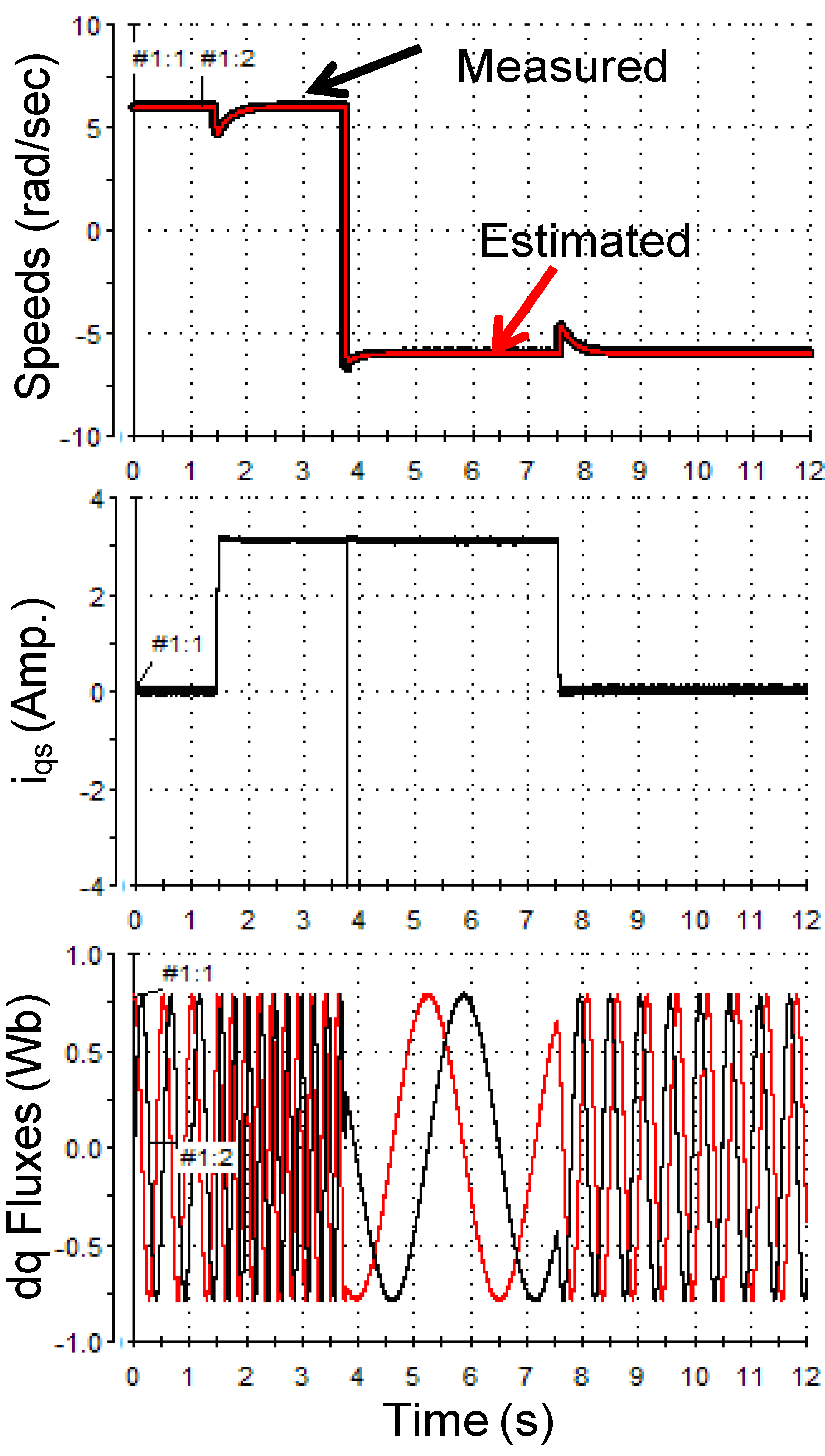
5.3. Fast Speed Reversal

The SIM drive using the designed OFGs was also examined during the performance at low-speed reversal. In the simulation results of Figure 15, the SIM drive worked in the motoring mode (forward) at a speed reference of 0.04 p.u (6.28 rad/s) during t = 0 to 2 s at T_L = 0. Then, a positive-rated T_L = +7 N.m at t = 2 s was applied. The speed reference was reversed to −0.04 p.u (−6.28 rad/s) at t = 4 s with rated load torque of T_L = +7 N.m. The SIM drive operated in the regenerating mode during t = 4 to 10 s with negative speed and positive load torque. The load torque was removed at t = 10 s. Then, SIM operated in the motoring mode (reverse) during t = 10 to 12 s at no-load torque. Identical experimental results are presented in Figure 16 with some differences in the time periods.

As is obvious, a significant convergence between the estimated speed and the actual one was achieved using with the proposed OFGs.

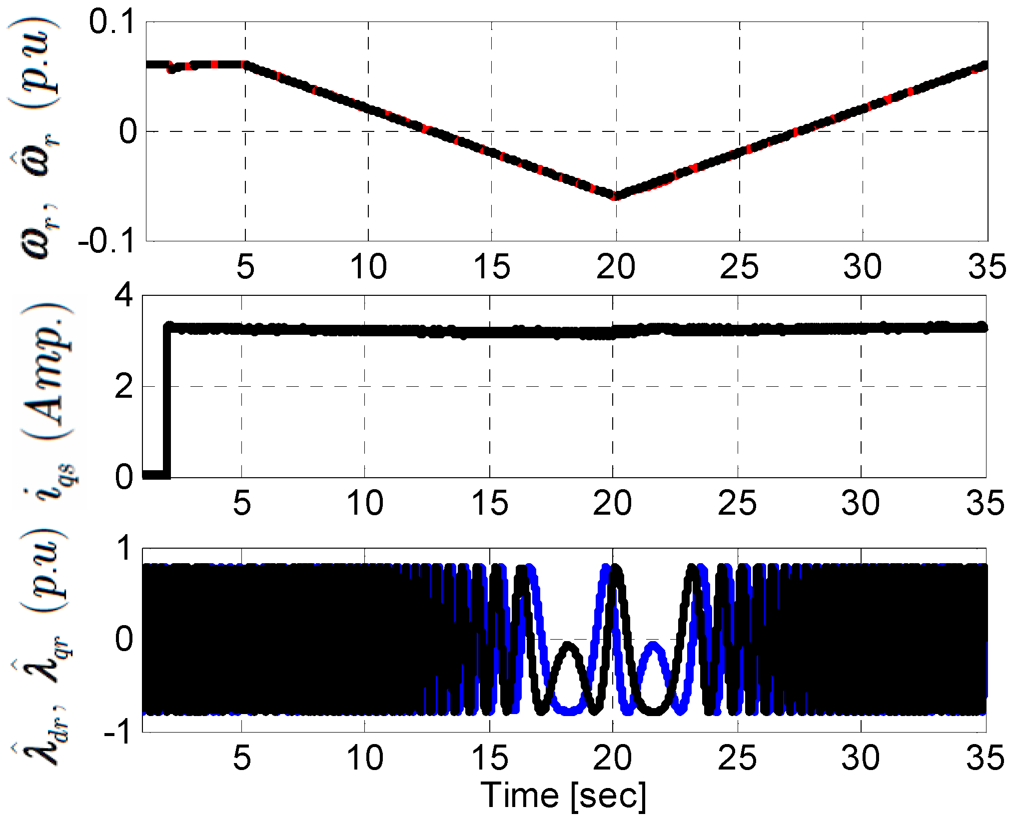
5.4. Slow Speed Reversal

The SIM drive using the designed OFGs was examined during the performance at slow speed reversal at low speeds. In the simulation results shown in Figure 17, the SIM drive operated in the motoring mode (forward) at a speed reference of 0.06 p.u (9.42 rad/s) during t = 0 to 1 s at no-load torque (T_L = 0). Then, a positive rated load torque of (T_L = +7 N.m) at t = 1 s was applied. The speed reference was slowly reversed to −0.06 p.u (−9.42 rad/s) at t = 5 s with rated load torque of T_L = +7 N.m at t = 20 s. Then, the speed reference was again slowly reversed to 0.06 p.u (9.42 rad/s) at t = 20 s with rated load torque of T_L = +7 N.m to t = 35 s. The SIM drive operated in the motoring mode, plugging mode, regenerating mode, and the plugging mode, and finally the motoring mode. Identical experimental results are presented in Figure 18 with some differences in the time periods. As is obvious, a significant convergence between the estimated speed and the actual one was achieved using with the proposed OFGs.

5.5. Zero Speed

The SIM drive with the proposed OFGs was examined during the performance at zero speed. As shown in the simulation results of Figure 19, the SIM drive operated at zero speed reference at no-load torque (T_L = 0). Then, a positive rated load torque of (T_L = +7 N.m) was applied at t = 4 s. Following this, the rated load torque of T_L = +7 N.m was removed at t = 12 s. Identical experimental results are presented in Figure 20. As is obvious, the SIM drive operated stably at zero speed using the proposed OFGs.

6. Comparison with Previous Works

To prove the efficacy of the optimal design of OFGs, the simulation and experimental results of Figure 17 and Figure 18 are presented in comparison to [23], (Figure 12 in [35]). It is evident that the proposed OFGs guaranteed a good performance during slow speed reversal.

Simulation and experimental results at zero speed are shown in Figure 19 and Figure 20, respectively. These figures shows the performance of the proposed OFGs in comparison to the designed AFO as in (Figure 9 in [21]), (Figure 12 in [23]), and (Figure 13 in [35]). As is obvious, the performance of the proposed OFGs is comparable with [21,23,35]. The stability was ensured during the operation in the unobservable region.

The proposed OFG-based AFO is an offline analytical method using GA and PSO optimization approaches. This is considered a limitation of the proposed method. Therefore, the designed OFG-based AFO by the offline method may not be working properly in online operations. This is the motivation for proposing a curve-fitting equation between the observer feedback gains and the deviations of stator resistance to guarantee the dominant zero location in the stable region.

In future work, GA and PSO optimization approaches will be designed and programmed as online optimization techniques of OFG-based AFO.

7. Conclusions

GA and PSO optimization approaches were used in this paper to design the OFGs of AFO. They were used to obtain the optimal OFGs to move the unstable dominant zero location under zero OFGs to the stable region during parameters’ mismatch in the regenerating mode of IM. The dominant zeros obtained by PSO had a superior location than that obtained by GA for both stator resistance and mutual inductance deviations. It was observed that the observer gain (K₂) had an almost constant value over a wide range of parameter deviations. However, the value of the observer gain K₁ was dependent on the deviation of machine parameters. The advantage of using PSO over GA was that the relation between the gain and parameter deviation can be represented by a deterministic and mostly linear relationship. The stability and accuracy of the SIM drive at very low speeds in the regenerating mode were proven using simulation and practical tests and compared with previous works. However, the proposed OFG-based AFO using GA or PSO techniques are offline analytical methods. Consequently, they may not be operating properly in an online real-time experimental system. This is considered a restriction of the proposed OFG-based AFO. A lock-up table will be considered in future work to determine the relation between the OFG-based AFO and the parameters’ deviation.

References

1. Pacas, M. Sensorless drives in industrial applications. IEEE Ind. Electron. Mag. 2011, 5, 16–23. [Google Scholar] [CrossRef]
2. Holtz, J. Sensorless control of induction machines—With or without signal injection? IEEE Trans. Ind. Electron. 2006, 53, 7–30. [Google Scholar] [CrossRef] [Green Version]
3. Kubota, H.; Matsuse, K.; Nakano, T. DSP-based speed adaptive flux observer of induction motor. IEEE Trans. Ind. Appl. 1993, 29, 344–348. [Google Scholar] [CrossRef]
4. Kubota, H.; Matsuse, K. Speed sensorless field-oriented control of induction motor with rotor resistance adaptation. IEEE Trans. Ind. Appl. 1994, 30, 1219–1224. [Google Scholar] [CrossRef]
5. Sun, W.; Yu, Y.; Wang, G. Design method of adaptive full order observer with or without estimated flux error in speed estimation algorithm. IEEE Trans. Power Electron. 2016, 31, 2609–2626. [Google Scholar] [CrossRef]
6. Xu, W.; Dian, R.; Liu, Y.; Hu, D.; Zhu, J. Robust flux estimation method for linear induction motors based on improved extended state observers. IEEE Trans. Power Electron. 2019, 34, 4628–4640. [Google Scholar] [CrossRef]
7. Devanshu, A.; Singh, M.; Kumar, N. An improved nonlinear flux observer based sensorless FOC IM drive with adaptive predictive current control. IEEE Trans. Power Electron. 2020, 35, 652–666. [Google Scholar] [CrossRef]
8. Alonge, F.; Cirrincione, M.; Pucci, M.; Sferlazza, A. A nonlinear observer for rotor flux estimation of induction motor considering the estimated magnetization characteristic. IEEE Trans. Ind. Appl. 2017, 53, 5952–5965. [Google Scholar] [CrossRef]
9. Zaky, M.S.; Metwaly, M.K.; Azazi, H.Z.; Deraz, S.A. A new adaptive smo for speed estimation of sensorless induction motor drives at zero and very low frequencies. IEEE Trans. Ind. Electron. 2018, 65, 6901–6911. [Google Scholar] [CrossRef]
10. Lascu, C.; Andreescu, G.-D. Sliding-mode observer and improved integrator with DC-offset compensation for flux estimation in sensorless-controlled induction motors. IEEE Trans. Ind. Electron. 2006, 53, 785–794. [Google Scholar] [CrossRef]
11. Suwankawin, S.; Sangwongwanich, S. A speed-sensorless IM drive with decoupling control and stability analysis of speed estimation. IEEE Trans. Ind. Electron. 2002, 49, 444–455. [Google Scholar] [CrossRef]
12. Suwankawin, S.; Sangwonwanich, S. Design Strategy of an Adaptive Full-Order Observer for Speed Sensorless Induction Motor Drives-Tracking Performance and Stabilization. IEEE Trans. Ind. Electron. 2006, 53, 96–119. [Google Scholar] [CrossRef]
13. HMaksoud, A.; Shaaban, S.M.; Zaky, M.S.; Azazi, Z.H. Performance and Stability Improvement of AFO for Sensorless IM Drives in Low Speeds Regenerating Mode. IEEE Trans. Power Electron. 2019, 34, 7812–7825. [Google Scholar] [CrossRef]
14. Saejia, M.; Sangwongwanich, S. Averaging analysis approach for stability analysis of speed-sensorless induction motor drives with stator resistance estimation. IEEE Trans. Ind. Electron. 2006, 53, 162–177. [Google Scholar] [CrossRef]
15. Zaky, M. Stability Analysis of Speed and Stator Resistance Estimators for Sensorless Induction Motor Drives. IEEE Trans. Ind. Electron. 2012, 59, 858–870. [Google Scholar] [CrossRef]
16. Zaky, M.; Metwaly, M.K. Sensorless Torque/Speed Control of Induction Motor Drives at Zero and Low Frequency with Stator and Rotor Resistance Estimation. IEEE J. Emerg. Sel. Top. Power Electron. 2016, 4, 1416–1429. [Google Scholar] [CrossRef]
17. Chang, C.-M.; Liu, C.-H. A new MRAS based strategy for simultaneous estimation and control of a sensorless induction motor drive. J. Chin. Inst. Eng. 2010, 33, 451–462. [Google Scholar] [CrossRef]
18. Harnefors, L.; Hinkkanen, M. Complete stability of reduced-order and full-order observers for sensorless IM drives. IEEE Trans. Ind. Electron. 2002, 55, 1319–1329. [Google Scholar] [CrossRef]
19. Kubota, H.; Sato, I.; Tamura, Y.; Matsuse, K.; Ohta, H.; Hori, Y. Regenerating-mode low-speed operation of sensorless induction motor drive with adaptive observer. IEEE Trans. Ind. Appl. 2002, 38, 1081–1086. [Google Scholar] [CrossRef]
20. Tsuji, M.; Chen, S.; Izumi, K.; Yamada, E. A sensorless vector control system for induction motors using q-axis flux with stator resistance identification. IEEE Trans. Ind. Electron. 2001, 48, 185–194. [Google Scholar] [CrossRef]
21. Hinkkanen, M. Analysis and design of full-order flux observers for sensorless induction motors. IEEE Trans. Ind. Electron. 2004, 51, 1033–1040. [Google Scholar] [CrossRef] [Green Version]
22. Etien, E.; Chaigne, C.; Bensiali, N. On the stability of full adaptive observer for induction motor in regenerating mode. IEEE Trans. Ind. Electron. 2010, 57, 1599–1608. [Google Scholar] [CrossRef]
23. Hinkkanen, M.; Luomi, J. Stabilization of regenerating-mode operation in sensorless induction motor drives by full-order flux observer design. IEEE Trans. Ind. Electron. 2004, 51, 1318–1328. [Google Scholar] [CrossRef] [Green Version]
24. Chen, B.; Wang, T.; Yao, W.; Lee, K.; Lu, Z. Speed Convergence Rate-Based Feedback Gains Design of Adaptive Full-Order Observer in Sensorless Induction Motor Drives. IET Electr. Power Appl. 2014, 8, 12–22. [Google Scholar] [CrossRef]
25. Orlowska-Kowalska, T.; Korzonek, M.; Tarchała, G. Stability Analysis of Selected Speed Estimators for Induction Motor Drive in Regenerating Mode—A Comparative Study. IEEE Trans. Ind. Electron. 2017, 64, 7721–7730. [Google Scholar] [CrossRef]
26. Yin, Z.; Zhang, Y.; Du, C.; Liu, J.; Sun, X.; Zhong, Y. Research on Anti-Error Performance of Speed and Flux Estimation for Induction Motors Based on Robust Adaptive State Observer. IEEE Trans. Ind. Electron. 2016, 63, 3499–3510. [Google Scholar] [CrossRef]
27. Sun, W.; Liu, X.; Gao, J.; Yu, Y.; Wang, G.; Xu, D. Zero Stator Current Frequency Operation of Speed-Sensorless Induction Motor Drives Using Stator Input Voltage Error for Speed Estimation. IEEE Trans. Ind. Electron. 2016, 63, 1490–1498. [Google Scholar] [CrossRef]
28. Orlowska-Kowalska, T.; Korzonek, M.; Tarchala, G. Stability Improvement Methods of the Adaptive Full-Order Observer for Sensorless Induction Motor Drive—Comparative Study. IEEE Trans. Ind. Inform. 2019, 15, 6114–6126. [Google Scholar] [CrossRef]
29. Sun, W.; Xu, D.; Jiang, D. Observability Analysis for Speed Sensorless Induction Motor Drives with and Without Virtual Voltage Injection. IEEE Trans. Power Electron. 2019, 34, 9236–9246. [Google Scholar] [CrossRef]
30. Sun, W.; Wang, Z.; Xu, D.G.; Yu, X.; Jiang, D. Stable Operation Method for Speed Sensorless Induction Motor Drives at Zero Synchronous Speed with Estimated Speed Error Compensation. IEEE Trans. Power Electron. 2019, 34, 11454–11466. [Google Scholar] [CrossRef]
31. Chen, J.; Huang, J.; Sun, Y. Resistances and Speed Estimation in Sensorless Induction Motor Drives Using a Model with Known Regressors. IEEE Trans. Ind. Electron. 2019, 66, 2659–2667. [Google Scholar] [CrossRef]
32. Chen, B.; Yao, W.; Chen, F.; Lu, Z. Parameter sensitivity in sensorless induction motor drives with the adaptive full-order observer. IEEE Trans. Ind. Electron. 2015, 62, 4307–4318. [Google Scholar] [CrossRef]
33. Hinkkanen, M.; Luomi, J. Parameter Sensitivity of Full-Order Flux Observers for Induction Motors. IEEE Trans. Ind. Appl. 2003, 39, 1127–1135. [Google Scholar] [CrossRef] [Green Version]
34. Hinkkanen, M.; Harnefors, L.; Luomi, J. Reduced-order flux observers with stator-resistance adaptation for speed-sensorless induction motor drives. IEEE Trans. Power Electron. 2010, 25, 1173–1183. [Google Scholar] [CrossRef]
35. Luo, C.; Wang, B.; Yu, Y.; Chen, C.; Huo, Z.; Xu, D. Operating-point tracking method for sensorless induction motor stability enhancement in low-speed regenerating mode. IEEE Trans. Ind. Electron. 2020, 67, 3386–3397. [Google Scholar] [CrossRef]
36. Sun, W.; Wang, Z.; Xu, D.; Wang, B. Robust stability improvement for speed sensorless induction motor drive at low speed range by virtual voltage injection. IEEE Trans. Ind. Electron. 2020, 67, 2642–2654. [Google Scholar] [CrossRef]
37. Morawiec, M.; Kroplewski, P.; Odeh, C. Nonadaptive rotor speed estimation of induction machine in an adaptive full-order observer. IEEE Trans. Ind. Electron. 2022, 69, 2333–2344. [Google Scholar] [CrossRef]
38. Zaky, M.S.; Fetouh, T.; Shaban, S.M.; Azazi, H.Z. A Novel Analytical Approach using Rough Set and Genetic Algorithm of a Stable Sensorless Induction Motor Drives in the Regenerating Mode. IEEE Access 2020, 8, 157748–157761. [Google Scholar] [CrossRef]
39. El-Ela, A.A.A.; Fetouh, T.; Bishr, M.A.; Saleh, R.A.F. Power System Operation using Particle Swarm Optimization Technique. Electr. Power Syst. Res. 2008, 78, 1906–1913. [Google Scholar] [CrossRef]
Figure 1. Block diagram of IFOC for a SIM drive with AFO. “*” means the reference variable.
Mathematics 10 01710 g001
Figure 2. Poles and zeros of G ω 22 s during the motoring mode of operation at low speed (20 rpm) and zero feedback gains (K1 = K2 = 0).
Mathematics 10 01710 g002
Figure 3. Poles and zeros of G ω 22 s during the regenerating mode of operation at low speed (20 rpm) and zero feedback gains (K1 = K2 = 0).
Mathematics 10 01710 g003
Figure 4. Optimal location of dominant zero in the regenerating mode using PSO and GA. (a) Under stator resistance deviation; (b) under magnetizing inductance deviation.
Mathematics 10 01710 g004
Figure 5. The optimal setting of observer feedback gains (K1 and K2) at different deviations in Rs and Lm using PSO. (a) Under stator resistance deviation; (b) under magnetizing inductance deviation.
Mathematics 10 01710 g005
Figure 6. The optimal setting of observer feedback gain K1 at different deviations in Rs and Lm using PSO.
Mathematics 10 01710 g006
Figure 7. Effect of deviation in Rs and superimposed effect of deviation in Lm on the observer feedback gain K1 using PSO. (a) Under stator resistance deviation; (b) under magnetizing inductance deviation.
Mathematics 10 01710 g007
Figure 8. Comparison between error measures for different design cases.
Mathematics 10 01710 g008
Figure 9. Simulation tests at low speeds. Speed reference of 0.04 p.u (6.28 rad/s) with rated TL change of +7 N.m at t = 2 s.
Mathematics 10 01710 g009
Figure 10. Practical tests at low speeds. Speed reference of 0.04 p.u (6.28 rad/s) with rated TL change of +7 N.m at t = 2 s.
Mathematics 10 01710 g010
Figure 11. Simulation tests at a speed reference of 0.08 p.u (12.56 rad/s) with rated TL change of −7 N.m at t = 2 s. Unstable AFO (K1 = K2 = 0).
Mathematics 10 01710 g011
Figure 12. Practical tests at a speed reference of 0.08 p.u (12.56 rad/s) with rated TL change of −7 N.m at t = 2 s. Unstable AFO (K1 = K2 = 0).
Mathematics 10 01710 g012
Figure 13. Simulation tests at a speed reference of 0.08 p.u (12.56 rad/s) with rated TL change of −7 N.m at t = 2 s.
Mathematics 10 01710 g013
Figure 14. Practical tests of at a speed reference of 0.08 p.u (12.56 rad/s) with rated TL change of −7 N.m at t = 2 s.
Mathematics 10 01710 g014
Figure 15. Simulation tests at a speed reference of 0.04 p.u (6.28 rad/s) was changed −0.04 p.u (−6.28 rad/s) with a rated TL change of +7 N.m applied at t = 2 s and removed t = 10 s.
Mathematics 10 01710 g015
Figure 16. Practical tests at a speed reference of 0.04 p.u (6.28 rad/s) was changed −0.04 p.u (−6.28 rad/s) with a rated TL change of +7 N.m applied at t = 2 s and removed t = 10 s.
Mathematics 10 01710 g016
Figure 17. Simulation tests at a speed reference of 0.06 p.u (9.42 rad/s) was changed slowly to −0.06 p.u (−9.42 rad/s) with an applied TL change of +7 N.m applied at t = 2 s.
Mathematics 10 01710 g017
Figure 18. Experimental tests at a speed reference of 0.06 p.u (9.42 rad/s) was changed slowly to −0.06 p.u (−9.42 rad/s) with an applied load torque change of +7 N.m applied at t = 2 s.
Mathematics 10 01710 g018
Figure 19. Simulation tests at speed reference of 0 p.u (0 rd/s) with rated load torque change of +7 N.m applied at t = 4 s and removed at t = 12 s.
Mathematics 10 01710 g019
Figure 20. Experimental tests at speed reference of 0 p.u (0 rd/s) with rated load torque change of +7 N.m applied at t = 4.5 s and removed at t = 12 s.
Mathematics 10 01710 g020