Warehouse Optimization: Energy Efficient Layout and Design

Abstract

It has been widely demonstrated by many research works that the distribution of a factory can condition its productivity. Because of this, a factory in Santiago, Chile, asked the authors for advice to evaluate the current situation in the company and what alternatives could be proposed to improve performance by increasing productivity without incurring too high costs. Among the most important requirements requested was a study of the current design of the raw materials warehouse within the plant since this is a main pillar in the design of the plant. For this purpose, the current layout ws analyzed and alternative designs were proposed under two scenarios: use the same area that is currently available or make the design from scratch considering land purchases to build the warehouse. In order to give a precise answer to many possible design decisions, formulations were developed and deduced to calculate the optimal dimensions of the warehouse, and qualitative criteria were incorporated for decision making.

1. Introduction

Nowadays, companies are challenged to redesign their processes and adapt to change. All this to improve the delivery and production of their goods and services. Among the most common strategic problems to be solved are those associated with the configuration of the supply chain [1] and how to tackle with supply chain risk [2]. The supply chain is the network of operations that manages the physical flow of materials, money and information throughout the entire purchasing, production, and distribution process, therefore, its configuration involves key elements such as facilities, transportation routes, cargo, storage areas, etc.

In this line, it has been shown that the planning of the design of facilities allows us to reduce costs, improve productivity, quality, and efficiency, giving us an overview of the current situation of the company and what we can do to achieve better scenarios.

In particular, this work deals with one key element of facility planning which is warehouse design. Since warehousing does not add value to the final product, the effort is placed on obtaining efficiency in costs, such as minimizing movements, workforce, equipment, and energy consumption, among other cost drivers.

From the sources review, starting in 2019, as to cite most recent works, several articles have focused on systematic literature reviews of the warehousing design problem [3,4]. Special issues in the production and operations management field have presented many works showing new problems and solutions [5,6] and novel methodologies [7].

In the literature we find several approaches to design, as in [8], where the design is planned through approaches with simulations and interactive design environments [9] which, although effective, mean high costs. Most works highlight the importance of design and how this concern has increased in recent years by the introduction of e-commerce, globalization, and new technologies such Internet and robotics ; these works, mainly focusing on address optimization algorithms to find better solutions or novel approaches to new problems, are applied in case studies [10]. For instance, in [11] a hierarchical design approach is presented; in [12], a new type of warehouse distribution, the fish-bone layout, is compared in performance; other works analyze changes in racks orientation and aisle design to move faster when performing order picking operations [13,14,15]. With the advent of e-commerce delivery operations and automation, new problems arise calling for intelligent warehouse or distribution center design [16].

Because of the different complexities involving warehouse design due to the variety of configurations and modes of operations, including stochastic demand patterns, chaotic storage and retrieval, among other factors, several works use simulation techniques, for instance, agent based modeling [17] and discrete event simulation combined with the design of experiments (DOE) [18,19].

In factories, warehouse design is one of the key areas to pay attention to since problems such as poorly designed facilities can cause excessive movements for product placement and picking, affecting customer service, delivery times, and increasing operational and labor costs. Although the works above are valuable, one problem from the practical point of view is the complexity of their implementation and they require considerable deployment of modeling skills and resources. For this reason, the main contribution of this work is to offer a closed-form solution that is easy to implement in industrial environments, drawing from experience in the field.

Previously in [20], the authors proposed formulas for the calculation of dimensions in the construction of warehouses, considering a given area in three dimensions; however, they are complex for implementation and limit the application only to known areas.

In this work, formulations for the energy efficient design of warehouses are deduced and proposed, which were developed for the calculation of the dimensions of a warehouse in a manufacturing company producing water heating appliances of two kinds: (a) fueled by LPG and (b) using electricity, the main water heating solution in the country and the Latin American region.

The formulations consider the construction of warehouses in two scenarios: restricted areas and unrestricted areas, with the objective that these found dimensions allow constructions that reduce the energy cost associated with the transportation of materials.

Then, in Section 2, the motivation and objectives of this work are detailed, where a little more about the situation of the company and the importance of design optimization are contextualized. Then in Section 3, the formulas for the calculation of dimensions are deduced and formally proposed, and in Section 4 they are tested with the factory that inspired this document. In Section 5, a case from the literature is taken to test the formulations deduced for the design of warehouses. Finally, in Section 6 the results obtained are analyzed and discussed, and then in Section 7 the conclusion is drawn.

2. Motivation and Objetives

In Chile and the world, the use of liquefied gas water heaters or heaters in private homes is common. Latin America is lagging in the energy transition race and will continue to use fossil fuel-based material moving equipment. As developed nations and Big Oil shareholders push for a faster transition to clean energy, much of Latin America is struggling just to meet its basic fossil fuel supply needs, which is forcing some countries to rely more on polluting energy sources. Experts speaking at the 2021 CERAWeek virtual conference, organized by IHS Markit, said that part of Latin America could be left behind in the energy transition due to outdated policies and ideas of resource nationalism, combined with the pressing need in some nations for cheap imported fuel [1]. At this time, as it is being accelerated by Big Oil companies and governments amid political pressure, Europe and now the United States have taken the lead through carbon neutral measures. “I do not see that aggressive policies in the energy matrix transition toward cleaner energy in Latin America”, said Decio Oddone, executive director of the Brazilian producer of petroleum and gas, Enauta S.A. As for the numbers, one could say that in 2018, Latin American nations together emitted as much carbon dioxide as Russia, the fourth largest emitter of CO₂ in the world, according to data from the International Energy Agency. The region has constantly increased the motor fuel import of natural gas, fuel oil, and diesel for power generation. In 2020, Latin America imported 2.69 million bpd of crude and refined products from the United States, its largest source of petroleum imports, according to a Reuters analysis based on data from the Energy Information Administration (EIA). According to the ECLAC transport division [2] in Chile, container handling oil and other liquid fuels accounted for 96% of all fuel consumption in 2014 and this country is a leader in the region on the issue of renewable energy. Motor gasoline continues to be the most used fuel in transportation, accounting for 39% of the total, while diesel follows closely in second place, with 36% in 2012. It is thus important to minimize the transfer of stored units, in order to cooperate within a cleaner industry. That is why the high demand and quality requirements for these products require continuous improvements within the production plants, to improve their performance and solve difficulties that often delay delivery times or hinder the work. In this context, the authors of this article were asked by a heater factory to provide a consultancy to evaluate the current design and distribution of the factory and proposals for redesign and improvements in one of its production plants located in Logroño, Estación Central, Chile.

Within the consultancy it was requested to evaluate the redesign of the finished products warehouse, evaluating two different scenarios: 1. use the space currently used as warehouse or 2. consider the purchase of new land to use and build it from scratch. At this stage is where the greatest complexity is generated since it was necessary to deduce and propose formulations for the calculation of the dimensions of this new warehouse whose objective is to minimize the distances traveled by the warehouse equipment.

Within the factory, materials are transported mainly by forklifts, which are very versatile vehicles and easy to maneuver in narrow spaces; however, careful planning of the transportation routes is required so that they do not interfere negatively with production activities. In addition, these cranes generate pollution during their use, so the objective was to minimize the movements of these cranes within the warehouse, which is directly associated with energy consumption. For this reason, it was proposed to minimize the energy expended when moving in the horizontal plane and at height.

3. Materials and Methods

Warehouse design is a process that considers two decisions: dimensions and inventory distribution. The efficiency of the warehouse will depend on this. The dimensions of the warehouse should be adjusted to the amount of inventory the company determines it should have, but it should also consider a prudent balance between height and width-length.

A warehouse with many levels in height decreases land expense; however, it is more difficult to maneuver, more effort is required to reach the inventory and, most importantly, there is a higher energy cost when transporting materials or inventory in vertical directions. On the other hand, if you choose to have a lower height warehouse, you must invest more in land to locate it, although the costs decrease inside the warehouse with transportation. Product movements are an important energy expense for the company, which can be minimized through design optimization.

Within the following formulas deduced for the design and distribution of warehouses, the movement factor was considered, and penalties were incorporated for vertical movement, preferring to travel horizontal distances. These features incorporated in design methodologies result in an energy efficient warehouse, where material movement costs are reduced and the distribution within the warehouse is improved according to the types of products inside.

To find the optimal dimensions and design, two study circumstances were used as explained in the previous section. These formulas are subject to a number of prior assumptions which are detailed below, which arise from the design of the warehouse in the plant of the consultancy carried out.

3.1. Assumptions

• The warehouse is rectangular (see Figure 1);
• Access to the factory is located at the top of the total area, while other facilities such as quality control and management are located at the bottom;
• Products will be stored on shelves on two sides except for the one adjacent to the wall;
• The aisle width will be the same for all aisles;
• Products enter the warehouse through the front door located on one of the longest walls on one side of the warehouse and exit through the opposite door (Figure 1).

These assumptions are based on the most used designs for warehouses, which are rectangular [6], with double racking to maximize capacity and space. On the other hand, only the orientation parallel to the longest part will be studied in this work due to the orientation of the warehouse in the consultancy used as a basis and given the limited literature available. It is believed that this type of design could set a precedent for the subsequent study of other warehouse orientations and shapes. By means of these assumptions, a simplified design commonly used in the world is analyzed.

Within the warehouse, the ABC method will be considered for the classification of inventories, so we will have three categories within: category A for the scarcest materials but which contribute to 80% of total profits, category B for products that represent 15% of sales and finally category C with 5%. This distribution policy considers the A products as those with the highest turnover, therefore, they will be the ones to be kept closer to periodically control the stock, since any stock rupture translates into large losses. On the opposite side for category C, we have products that generate low income and which we will have fewer resources to control.

With these considerations in the following section, we deduce the formulas used.

3.2. Case 1: Design of a Given Area

The objective is to model the energy use for moving products within the warehouse. Therefore, we will use Figure 1 as a schematic to refer to the dimensions and orientation of the warehouse. First, length $t_v$ and width $t_u$ of the warehouse will be calculated using Equations (1) and (2). The total width of the warehouse is $t_u$ in Figure 1:

$$t_u=n_u(w+c).$$

(1)

In addition, the total length of the warehouse is $t_v$, considering Figure 1 as [21]:

$$t_v=2c+ml.$$

(2)

Considering that both length and width restrict the cost of transporting and handling the goods inside the warehouse, the warehouse area (DC) has the dimension given by Equation (3).

$$Area=t_u\ast t_v=n_u(w+c)\ast (2c+n_{u}l).$$

(3)

The expected value of the travel distance is used to obtain an energy consumption function as a function of the distance covered. To calculate the warehouse cost function, the expected value of the distances covered on the horizontal plane is defined as $E(d_v)$ and $E(d_u)$, and on the vertical axis as $E(d_h)$. As indicated above, the doors are located in the middle of the longest wall, therefore, the distance covered in $\overrightarrow{u}$ is at most $t_u$/2. On average, this would be half of that amount, i.e., $t_u$/4, as shown in Equation (4) for the expected distance.

$$E(d_u)=\frac{t_u}{4}=\frac{n_u(e+c)}{4}$$

(4)

$${\Omega }_u:1,...,\left[\frac{t_u}{2}\right]$$

Measuring the distance covered in direction $\overrightarrow{v}$ depends on the category of the goods. Because category A goods are stored in the first part of the warehouse because they have a higher turnover; category B goods are stored in the second part and category C goods are stored in the last part, farther away. The number of storage spaces is $m_A$ for category A, which is why the average distance covered is $m_A$/2, therefore, the expected value of distance covered by an element of category A, $E(d_A)$ is given by Equation (5).

$$E(d_A)=\frac{m_{A}l}{2}=\frac{n_u(w+c)}{4}$$

(5)

$${\Omega }_A=1,...,m_{A}l$$

Then, for category B, first consider the distance covered in the first part for type A inventory and then follow the analogous procedure to obtain the average distance as shown in (6).

$$E(d_B)=m_{A}l+\frac{m_{B}l}{2}$$

(6)

$${\Omega }_B=1,...,m_{A}l+\frac{m_{B}l}{2}$$

Likewise, the expected value for the distance covered per category C article will be called $E(d_C)$, corresponding to the equation expressed in (7).

$$E(d_c)=m_{A}l+m_{B}l+\frac{m_{C}l}{2}$$

(7)

$${\Omega }_C=1,...,m_{A}l+m_{B}l+\frac{m_{C}l}{2}$$

With this formulation, the expected value of the travel distance of any item in direction $\overrightarrow{v}$ is given by Equation (8).

$$E(d_v)=\alpha +P_{rA}E(d_A)+P_{rB}E(d_B)+P_{rC}E(d_C).$$

(8)

Replacing $E(d_A)$, $E(d_B)$ and $E(d_C)$ in Equation (8) an expression for $E(d_v)$, we obtain Equation (9).

$$E(d_v)=\alpha +l(P_{rA}\frac{m_A}{2}+P_{rB}{m}_A+P_{rB}\frac{m_B}{2}+P_{rC}{m}_A+P_{rC}{m}_B+P_{rC}\frac{m_C}{2}).$$

(9)

By property of probabilities, it contains Equation (10).

$$P_{rA}+P_{rB}+P_{rC}=1.$$

(10)

The total capacity of the warehouse to store articles of categories A, B, and C can be expressed as follows in (11)–(13):

$$N_A=2m_A{n}_u{n}_h$$

(11)

$$N_B=2m_B{n}_u{n}_h$$

(12)

$$N_C=2m_C{n}_u{n}_h.$$

(13)

Finally, Equation (14) shows the expected value of the distance traveled in height, which is at most $n_h$, which on average is $n_h$/2.

$$E(d_h)=\frac{n_h}{2}.$$

(14)

The energy consumption equation for a warehouse with the ABC Method is as in Equation (15).

$$Energy=4d{E}_{\mu }(c+l(P_{rA}\frac{m_A}{2}+P_{rB}{m}_A+P_{rB}\frac{m_B}{2}+P_{rC}{m}_A+P_{rC}{m}_B+P_{rC}\frac{m_C}{2})$$

(15)

$$+\frac{n_u(w+c)}{4}+(2d{E}_{\mu }{F}_h)\frac{n_h}{2})$$

The term (15) depends on variables $m_A$, $m_B$, $m_C$, $n_u$ and $n_h$. Term $F_h$ is the energy cost penalty height factor for the movement of load in altitude. According to the cost data considered, we have estimated $F_h=3$. By considering and adding the constraints, the system can be expressed as follows, in (16) to (21).

Problem 1.

$$Mi{n}_{m_A,m_B,m_C,n_u,n_h}\left\{Energy\right\}$$

(16)

Subject to Equations (11)–(13) and:

$$n_u(w+c)=t_u$$

(17)

$$2c+l(m_A+m_B+m_C)=t_v$$

(18)

This is solved by transforming the system as a Lagrangian function, where we obtain Equation (22).

$$L_g=4d{E}_{\mu }(c+l(P_{rA}\frac{m_A}{2}+P_{rB}{m}_A+P_{rB}\frac{m_B}{2}+P_{rC}{m}_A+P_{rC}{m}_B+P_{rC}\frac{m_C}{2})+$$

(19)

$$\frac{n_u(w+c)}{4}+(2d{E}_{\mu }{F}_h)\frac{n_h}{2})+{\lambda }_u[t_u-n_u(w+c)]+{\lambda }_v[t_v-2c+l(m_A+m_B+m_C)]$$

$$+{\lambda }_A[N_A-2m_A{n}_u{n}_h]+{\lambda }_B[N_B-2m_B{n}_u{n}_h]+{\lambda }_C[N_C-2m_C{n}_u{n}_h]$$

Five new variables result in this new function as a product of the Lagrange function formation. Three of them, ${\lambda }_A$, ${\lambda }_B$ and ${\lambda }_C$, are related to the time slots of categories A, B, and C, respectively. On the other hand, the other two variables, ${\lambda }_u$ and ${\lambda }_v$, are related to the dimensions of the rectangular warehouse space $t_u$ and $t_v$. Partially differing with regard to variables $m_A$, $m_B$, $m_C$, $n_u$, $n_h$ and then equating to zero to find the minimum of the function and thus the minimum dimensions required, we obtain Equations (23) to (32).

$$\frac{\partial L_g}{\partial m_A}=4d{E}_{\mu }l(\frac{P_{rA}}{2}+P_{rB}+P_{rC})+{\lambda }_{v}l-2n_u{n}_h{\lambda }_A=0$$

(20)

$$\frac{\partial L_g}{\partial m_B}=4d{E}_{\mu }l(\frac{P_{rB}}{2}+P_{rC})-{\lambda }_{v}l-2n_u{n}_h{\lambda }_B=0$$

(21)

$$\frac{\partial L_g}{\partial m_C}=4d{E}_{\mu }l\frac{P_{rC}}{2}-{\lambda }_{v}l-2n_u{n}_h{\lambda }_C=0$$

(22)

$$\frac{\partial L_g}{\partial n_u}=4d{E}_{\mu }l\frac{(w+c)}{4}-{\lambda }_u(w+c)-{\lambda }_{A}2m_A{n}_h-{\lambda }_{B}2m_B{n}_h-{\lambda }_{C}2m_C{n}_h=0$$

(23)

$$\frac{\partial L_g}{\partial n_h}=\frac{2d{E}_{\mu }A}{2}-2m_A{n}_u{\lambda }_A-2m_B{n}_u{\lambda }_B-2m_c{n}_u{\lambda }_c=0$$

(24)

$$\frac{\partial L_g}{\partial {\lambda }_A}=N_A-2m_A{n}_u{n}_h=0$$

(25)

$$\frac{\partial L_g}{\partial {\lambda }_B}=N_B-2m_B{n}_u{n}_h=0$$

(26)

$$\frac{\partial L_g}{\partial {\lambda }_C}=N_C-2m_C{n}_u{n}_h=0$$

(27)

$$\frac{\partial L_g}{\partial {\lambda }_u}=T_u-n_u(w+c)=0$$

(28)

$$\frac{\partial L_g}{\partial {\lambda }_v}=T_v-2c+l(m_A+m_B+m_C)=0.$$

(29)

Multipliers ${\lambda }_A$, ${\lambda }_B$ and ${\lambda }_C$ measure the scarcity of the corresponding resource, either in A, B, or C. They are also called shadow prices, representing the opportunity cost of using space for this item. By clearing ${\lambda }_A$, ${\lambda }_B$, and ${\lambda }_C$ of the above equations, we obtain the Equations (33)–(35) for the shadow prices.

$${\lambda }_A=\frac{l(2d{E}_{\mu }(2-P_{rA})-{\lambda }_v)}{2n_u{n}_h}$$

(30)

$${\lambda }_B=\frac{l(2d{E}_{\mu }(P_{rB}+2P_{rC})-{\lambda }_v)}{2n_u{n}_h}$$

(31)

$${\lambda }_C=\frac{l(2d{E}_{\mu }{P}_{rC}-{\lambda }_v)}{2n_u{n}_h},$$

(32)

where ${\lambda }_u$ and ${\lambda }_v$ represent the scarcity of the resource regarding width and length. By clearing ${\lambda }_u$ and ${\lambda }_v$ of Equations (23) to (32) we obtain Equations (36) and (41).

$${\lambda }_v={\lambda }_u.$$

(33)

Finally, by clearing the variables, we obtain the dimensions sought for this first case:

$$n_u=\frac{T_u}{w+c}$$

(34)

$$n_h=\frac{N_A+N_B+N_C}{n_u(w+c)m}$$

(35)

$$m_A=\frac{N_A}{2n_u{n}_h}$$

(36)

$$m_B=\frac{N_B}{2n_u{n}_h}$$

(37)

$$m_C=\frac{N_C}{2n_u{n}_h}$$

(38)

Then we correct the Formulas (39) to (41) to adjust them to the given area.

$$f_c=\frac{t_v-2c}{lm}$$

(39)

And then we have:

$$m_A^{corr}=m_A\ast f_c$$

(40)

$$m_B^{corr}=m_B\ast f_c$$

(41)

$$m_C^{corr}=m_C\ast f_c$$

(42)

$$n_h^{corr}=n_h\ast f_c$$

(43)

3.3. Case 2: Design of an Unrestricted Area

In the previous case, since $T_u$ and $T_v$ are given a priori, the values of m and n are also fixed a priori, so that the only variable that determines the system is the number of spaces at height h. Therefore, there is no need to penalize movement in height, as the spaces are allocated so that the required load is complete. In the second case, the measurements on the horizontal plane are not defined a priori. In this way, the system of equations must determine three values of the number of spaces on the X-axis, Y-axis, and Z-axis. It is therefore important to properly penalize movement in height. The mean movement on the vertical axis is given by the Equation (42).

$$E(d_h)=\frac{n_h}{2}.$$

(44)

In [21], an interesting approach proposes to use an exponential function as in Equation (43), because the expected displacement increases exponentially, such as the height of the shelves or, in this case, the height of the space for the items. It is also stated that a linear function seems inappropriate for modeling the increase in storage equipment or investment, so this exponential approximation is used.

$$E(d_h)=e^{\frac{h}{2}}.$$

(45)

However, in doing so, the Lagrangian system does not reveal the variables directly, making it an implicit system of equations. Therefore, we have considered using an approximate quadratic function (44) representing the average distance covered from two points: the ground and the maximum represented by h.

$$E(d_h)=F_h=\frac{h^2}{2}.$$

(46)

This function approximates the values of the exponential. However, for very high height values, we obtain values that are lower than the real ones. The comparison of both variables is shown in the following chart (Figure 2).

For values of h greater than 7 we can observe that the approximation of the quadratic function is less accurate, as it underestimates the expected distance covered. However, between 7 and 8 m is the maximum height at which maneuvering inside the warehouse is not difficult.

Analogously following the procedure of the previous case, we obtain the new expression of the energy expenditure given by Equation (45), restricted by Equations (11)–(13), (47) and (48).

$$Energy=4d{E}_{\mu }(c+l(P_{rA}\frac{m_A}{2}+P_{rB}{m}_A+P_{rB}\frac{m_B}{2}+P_{rC}{m}_A+P_{rC}{m}_B+P_{rC}\frac{m_C}{2})$$

(47)

$$+\frac{n_u(w+c)}{4}+(2d{E}_{\mu }{F}_h)\frac{n_h}{2})$$

And subject to Equations (11)–(13).

With a Lagrangian given by Equation (49).

$$L_g=4d{E}_{\mu }(c+l(P_{rA}\frac{m_A}{2}+P_{rB}{m}_A+P_{rB}\frac{m_B}{2}+P_{rC}{m}_A+P_{rC}{m}_B+P_{rC}\frac{m_C}{2})+$$

(48)

$$\frac{n_u(w+c)}{4}+(2d{E}_{\mu }{F}_h)\frac{n_h}{2})+{\lambda }_u[t_u-n_u(w+c)]+{\lambda }_A[N_A-2m_A{n}_u{n}_h]$$

$$+{\lambda }_B[N_B-2m_B{n}_u{n}_h]+{\lambda }_C[N_C-2m_C{n}_u{n}_h]$$

Partially deriving as a function of variables $m_A$, $m_B$, $m_C$, $n_u$, $n_h$, ${\lambda }_A$, ${\lambda }_B$ and ${\lambda }_C$, Equations (50) to (57) are obtained.

$$\frac{\partial L_g}{\partial m_A}=4d{E}_{\mu }l(\frac{P_{rA}}{2}+P_{rB}+P_{rC})-2n_u{n}_h{\lambda }_A=0$$

(49)

$$\frac{\partial L_g}{\partial m_B}=4d{E}_{\mu }l(\frac{P_{rB}}{2}+P_{rC})-2n_u{n}_h{\lambda }_B=0$$

(50)

$$\frac{\partial L_g}{\partial m_C}=4d{E}_{\mu }l\frac{P_{rC}}{2}-2n_u{n}_h{\lambda }_C=0$$

(51)

$$\frac{\partial L_g}{\partial n_u}=4d{E}_{\mu }l\frac{(w+c)}{4}-{\lambda }_{A}2m_A{n}_h-{\lambda }_{B}2m_B{n}_h-{\lambda }_{C}2m_C{n}_h=0$$

(52)

$$\frac{\partial L_g}{\partial n_h}=\frac{2d{E}_{\mu }A}{2}-2m_A{n}_u{\lambda }_A-2m_B{n}_u{\lambda }_B-2m_C{n}_u{\lambda }_C=0$$

(53)

$$\frac{\partial L_g}{\partial {\lambda }_A}=N_A-2m_A{n}_u{n}_h=0$$

(54)

$$\frac{\partial L_g}{\partial {\lambda }_B}=N_B-2m_B{n}_u{n}_h=0$$

(55)

$$\frac{\partial L_g}{\partial {\lambda }_C}=N_C-2m_C{n}_u{n}_h=0$$

(56)

This value indicates how important the space is for the articles of category A, it is estimated that category B should be half as important as category A and category C half as important as category B. According to this you have:

Finally, the design variables obtained are shown in (63) to (71).

$${\lambda }_A=\frac{d{E}_{u}lA{n}_h}{N_A+N_B+N_C}$$

(57)

$${\lambda }_B=0.5{\lambda }_A$$

(58)

$${\lambda }_C=0.5{\lambda }_B$$

(59)

$$n_u=\frac{T_u-2C}{c+w}$$

(60)

$n_h$ It´s a data, it is fixed a priori, according to the height available.

$${\lambda }_v=\frac{4d{E}_{u}l(\frac{P_b}{2}+P_c)-n_{h}4d{E}_{u}l(\frac{P_a}{2}+P_b+P_c)}{l+n_h}$$

(61)

$${\lambda }_u=4d{E}_{u}l\frac{(w+c))}{4}-\frac{{\lambda }_A{N}_A+{\lambda }_B{N}_B+{\lambda }_C{N}_C}{n_u(w+c)}$$

(62)

$$m_A=\frac{N_A}{2n_u{n}_h}$$

(63)

$$m_B=\frac{N_B}{2n_u{n}_h}$$

(64)

$$m_C=\frac{N_C}{2n_u{n}_h}$$

(65)

4. Factory Testing

In this section, we present the application of the formulations proposed above. We begin by briefly characterizing and analyzing the configuration of the work plant, and then defining the variables and parameters used in the development of the case.

4.1. Factory Setup

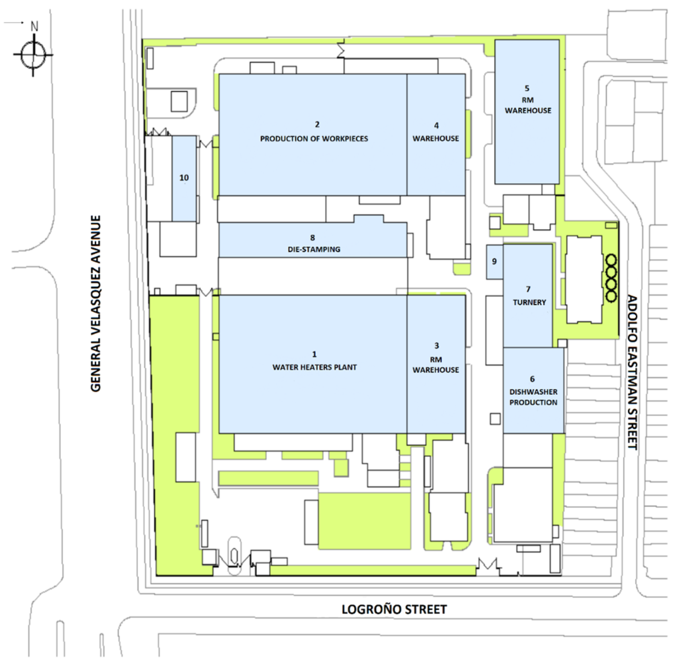
In Figure 3, the colors represent: The green color is used for transit of people, light blue is for closed work spaces, and white color is for truck, crane traffic and other vehicules. Section 9 corresponds to the tooling area and section 10 to the administrative staff offices. As shown in Figure 3, the factory located at the intersection of Adolfo Eastman and Logroño streets is a large production plant with different processes running simultaneously for the manufacture of water heaters, where sinks and spare parts are also manufactured for sale. These areas include have the finished product warehouse which is a fundamental pillar in the production of all items in the factory. The following flow chart shows the role of this area within the plant.

The flow chart in Figure 4 shows all the flows of materials, finished products and products in process in one month, measured in tons. Given the distribution of these flows, we can corroborate the previous premise, where the warehouses of both finished products and finished products are fundamental pillars of production. In this case, we will analyze the finished product warehouse specifically, which is where the greatest movement of the company takes place, given the different models with their respective capacities for sale and the company’s demand.

4.2. Application

The formulas developed in Section 3 are validated here. The warehouse manages three product families, water heaters with 16 L (A), 13 L (B) and 8 L (C) capacity. All products stored in the warehouse are classified into one of these three categories according to the ABC categories. Thus, products in category A are located closer to the door, while those in class B are at a medium distance and those in class C are at a greater distance. The probability of belonging to class A is 0.5, of belonging to class B is 0.3, and of belonging to class C is 0.2, giving greater weighting to the most important classification. The warehouse is organized by classes according to the ABC Method, with the following segmentation: 4125 ($n_A$), 2475 ($n_B$) and 990 ($n_c$), which correspond to the spaces allocated for storage by product class. Regarding the dimensions of the warehouse, frames with loading on both sides are available, width (w) of 2.2 m. Each storage space measures a width of 1.1 m and a height of 1 m. Aisle width is 2 m and door width is 4 m. Finally, the demand is estimated at 120,000 pallets of products per year and the warehouse capacity is 7590 pallets. A summary of the parameters and their values is presented below in the

Table 1. Summary of parameters and their values in the water heater factory.

Parameter	Value
l (m)	1.0
$\alpha$ (m)	2.0
N (pallets)	7590
d (pallets)	120,000
$E_{\mu }$ (US$/meter)	0.0069
$N_A$	4125
$N_B$	2475
$N_C$	990
$P_{rA}$	0.5
$P_{rB}$	0.3
$P_{rC}$	0.2
w (m)	2.2
$F_h$	3

.

The values for the cost of movement on the horizontal plane $E_{\mu }$ and the height penalty factor $F_h$ were estimated from the company’s accounting records.

5. Results

5.1. Results of the Case 1: Design of a Given Area

The distance covered towards one of the axes is, in this case, $T_u$ = 42 m and $T_v$ = 20 m. The results obtained for the restricted case are shown in

Table 2. Results obtained using formulas for the restricted case.

Values	${\mathit{n}}_{\mathit{u}}$	${\mathit{n}}_{\mathit{h}}$	${\mathit{m}}_{\mathit{A}}$	${\mathit{m}}_{\mathit{B}}$	${\mathit{m}}_{\mathit{C}}$	m	${\mathit{T}}_{\mathit{u}}$ Calculated	${\mathit{T}}_{\mathit{v}}$ Calculated
Obtained	9.523	11.859	10.075	4.231	1.692	16.001	42	42
Rounded	10	12	11	5	2	18	42	42

. This table shows that the height of the warehouse reaches 25 storage spaces, measuring l = 1.0 m each, which gives a heat of 25 metros. It is therefore necessary to evaluate the possibility of using a free floor plan such as that in case 2. The results to be considered for the warehouse facility design are rounded to the nearest integer, without exceeding the available site dimensions given by $T_u$ and $T_v$.

Fixing the value of height $n_h$ the rest of the variables are obtained, it can be observed that due to the rounding of variables the dimension of $T_u$ exceeded the given value.

5.2. Results of the Case 2: Design of an Unrestricted Area

The results obtained for the case of the unrestricted system are shown in

Table 3. Results obtained using formulas for the case without restrictions.

Values	${\mathit{n}}_{\mathit{u}}$	${\mathit{n}}_{\mathit{h}}$	${\mathit{m}}_{\mathit{A}}$	${\mathit{m}}_{\mathit{B}}$	${\mathit{m}}_{\mathit{C}}$	m	${\mathit{T}}_{\mathit{u}}$ Calculated	${\mathit{T}}_{\mathit{v}}$ Calculated
Obtained	16.59	8	15.535	9.321	3.728	28.584	69.701	32.585
Rounded	17	8	16	10	4	30	70	33

. The rounding was performed by approximating the upper integer values of $n_h$ and $m_A$. This is because we decided to evaluate the worst-case scenario to avoid overestimations and effects that would not occur. Table 3 shows that the measurements differ from those of Table 2, which shows the case of a restricted surface. In the case of a free area, the value of $n_h$ is significantly lower than the restricted case, which is explained due to the possibility of expanding laterally instead of towards the roof. The opposite occurs with the term $m_B$, which increases by 6 units, while $m_C$ increases by 1 unit.

By freeing up the available space and setting the number of slots in height at 8, with which one obtains a used area of 840 square meters in the restricted case is increased to 2.310 m${}^2$, which is 2.5 times greater.

6. Others Results

In order to validate the developed formulas and verify that they present some degree of generality, they were applied to the calculation of shelves in two case studies of Chilean companies, one corresponding to the Glavima company, from the metalworking sector that manufactures industrial machinery, and the Kupfer company dedicated to for sale of hydraulic spare parts cutting equipment and personal protection element.

Glavima is a company in the metalworking area dedicated to the design, manufacture and installation of industrial machinery and equipment. It has 98 employees and various departments, including machining, tooling, structures, production facilities and quality control. The warehouse is small in size, being and area of 15 × 5 m.

Applying the formulas to the design of shelves in the current given area of 15 by 5 m${}^2$, the following results are obtained and are showed in the

Table 4. Results of applying the formulas to the warehouse of the Glavima company with area restriction.

Values	${\mathit{n}}_{\mathit{u}}$	${\mathit{n}}_{\mathit{h}}$	${\mathit{m}}_{\mathit{A}}$	${\mathit{m}}_{\mathit{B}}$	${\mathit{m}}_{\mathit{C}}$	m	${\mathit{T}}_{\mathit{u}}$ Calculated	${\mathit{T}}_{\mathit{v}}$ Calculated
Obtained	15	13.711	6.499	2.082	0.599	9.18	15	5.5
Rounded	15	14	7	3	1	11	15	6

.

If more space were available, this would allow lowering the number of shelves in height, for example to a value of 8 levels, that is $n_h=8$. With this value the results are as follows in the

Table 5. Results of applying the formulas to the warehouse of the Glavima company without area restriction.

Values	${\mathit{n}}_{\mathit{u}}$	${\mathit{n}}_{\mathit{h}}$	${\mathit{m}}_{\mathit{A}}$	${\mathit{m}}_{\mathit{B}}$	${\mathit{m}}_{\mathit{C}}$	m	${\mathit{T}}_{\mathit{u}}$ Calculated	${\mathit{T}}_{\mathit{v}}$ Calculated
Obtained	2.905	8	29.262	8.821	2.539	40.622	3.922	18.055
Rounded	3	8	30	9	3	41	4	19

.

Now you can see that by setting the number of levels to a lower value, you have a more extended warehouse with a length of 4 by 19 m.

“Kupfer” is a Chilean company that markets a wide range of products focused on different productive industries nationwide. Its product offering corresponds mainly to: hydraulic spare parts, cutting equipment, lifting materials, personal protection elements, among others. This company has been in the Chilean industrial market for approximately 140 years, with an important position as a result of the trust and prestige earned during its history. It currently has a central warehouse of more than 5000 square meters.

The

Table 6. Results of applying the formulas to the warehouse of the Kupfer company with area restriction.

Values	${\mathit{n}}_{\mathit{u}}$	${\mathit{n}}_{\mathit{h}}$	${\mathit{m}}_{\mathit{A}}$	${\mathit{m}}_{\mathit{B}}$	${\mathit{m}}_{\mathit{C}}$	m	${\mathit{T}}_{\mathit{u}}$ Calculated	${\mathit{T}}_{\mathit{v}}$ Calculated
Obtained	12.766	22.279	45.377	6.502	4.121	56	61.1	71.2
Rounded	13	23	46	7	5	58	62	72

shows the results of applying the formulas to the unrestricted case.

The

Table 7. Results of applying the formulas to the warehouse of the Kupfer company without area restriction.

Values	${\mathit{n}}_{\mathit{u}}$	${\mathit{n}}_{\mathit{h}}$	${\mathit{m}}_{\mathit{A}}$	${\mathit{m}}_{\mathit{B}}$	${\mathit{m}}_{\mathit{C}}$	m	${\mathit{T}}_{\mathit{u}}$ Calculated	${\mathit{T}}_{\mathit{v}}$ Calculated
Obtained	4.057	10	24.760	2.818	1.453	29.031	13.522	62.062
Rounded	5	10	25	3	2	30	14	63

shows the results of applying the formulas to the warehouse of the Kupfer company without area restriction.

Now, by having a restricted area, the measurement in the $\overrightarrow{u}$ direction drastically decreased to 14 units, from 62 in the restricted case.

7. Discussion

With the tests performed, it can be concluded that the formulas developed in this work contribute to an explicit, simple and direct calculation for the dimensions of a warehouse, providing quality solutions in terms of minimizing energy consumption for transporting materials.

First we analize the warehouse of the water heater factory obtained for the case with restricted area, we find that this particular area of 40 m wide and 20 m high creates a dimension that allows the construction of an energy efficient warehouse, given the limitations, although they make the warehouse must have more height than the ideal, with a total height of 25 m, which will hinder the handling of inventory in height and especially increase energy costs. An advantage of these formulas is that they allow the calculation of values and foresee the difficulty associated with such a high warehouse.

On the other hand, comparing with the unrestricted case, it can be observed that an increase of resource, in this case space on the $\overrightarrow{u}$ axis (length), can considerably vary the amount of height of the warehouse, so it is not always necessary to acquire new land to make the warehouse from scratch, opening the possibility of extending the existing land to the meters required to achieve an optimal design of low consumption; in this case, an increase of 55 m in width allows a decrease by 17 m in height from the delimited area to the unrestricted area. It is necessary to balance in each case the costs of land acquisition with the costs of energy consumption that are raised in height, project them over a period of time, and make an evaluation of the projects to see their suitability.

The two warehouses shown in Section 6 are of different types, the warehouse of the GLAVIMA company is small like the company dedicated to metalworking and industrial projects. It stores medium and small size tools so it has small size containers. The KUPFER company stores truck parts and therefore has larger containers. In both cases the formulas worked well and proved to be valid for a wide range of warehouses. The warehouses are an area of great movement, and it is here where the greatest fuel consumption occurs, in addition, as for this test the transport is developed with fork cranes, large displacements also contribute to labor fatigue of workers so that these effects are also diminished. The values presented can be used to evaluate the factory ideal for industries of any type, not only dedicated to the manufacture of heaters as in the case study presented.

Finally, it is necessary to analyze that the contribution of these formulations is not limited only to the calculation of dimensions, but that the penalties play an important role as indicators within the distribution of the warehouse. These guide us on the internal distribution of the categories, where increases or decreases of the spaces destined to these can harm or contribute to the decrease of the energy consumption per movement, which is our objective to minimize.

It is proposed for future research to study other distributions and forms of warehouses taking these formulations as a basis to be able, finally, to expand the results to any type of warehouse to be built. In addition, an interesting approach proposed is to incorporate the design of warehouses within the design methodologies of production plants, since this way the flows within the production process are improved and efficient designs can be deduced.

8. Annexes

The

Table 8. Calculation with free area.

Definition	Parameter/Variable	Cem	Kupfer	Glavima
Number of shelves in height a priori.	$n_h$	8	10	8
Number of category A items.	$N_A$	4125	2232	1360
Number of category B items.	$N_B$	2475	254	410
Number of category C items.	$N_C$	990	131	118
Wide of double shelf.	w	2.2	1	0.65
Aisle.	c	2	2	0.7
Annual demand d.	d	120,000	2198	11326
Energy spent.	$E_u$	0.0069	0.0073	0.073
Height of the container.	l	1	2	0,41
Probability category A.	$P_A$	0.5	0.85	0.72
Probability category B.	$P_B$	0.3	0.097	0.22
Probability category C.	$P_C$	0.2	0.0501	0.06
Number of shelves in u direction.	$n_u$	16,595	4507	2905
Number of shelfs of category A.	$m_A$	15,535	24,760	29,262
Number of shelfs of category B.	$m_B$	9321	2818	8821
Number of shelfs of category C.	$m_C$	3728	1453	2539
Total number of shelfs.	m	28,585	29,031	40,622
$T_u$ calculated.	$T_u$	69,701	13,522	3922
$T_v$ calculated.	$T_v$	32,585	62,062	18,055

shows the parameters and values obtained applying the formulas developed for the case of free area.

The

Table 9. Calculation with restricted area.

Definition	Parameter/Variable	Cem	Kupfer	Glavima
Given width in u direction	$T_u$ given	40	60	15
Given width in u direction	$T_v$ given	20	60	10
Number of category A items	$N_A$	4125	52,173	1360
Number of category B items	$N_B$	2475	13,884	410
Number of category C items	$N_c$	990	8799	118
Wide of double shelf	w	2.2	2.7	0.59
Aisle	c	2	2	0.41
Annual demand d	d	120,000	39,315,678	11,326
Energy spent	$E_u$	0.0069	0.0073	0.073
Height of the container	l	1	1.2	0.51
Probability of category A	$P_A$	0.5	0.85	0.72
Probability of category A	$P_B$	0.3	0.097	0.22
Probability of category A	$P_C$	0.2	0.0501	0.06
Number of shelves in u direction	$n_u$	9524	12,766	15
Number of shelves in height a priori	$n_h$	3862	3463	7867
Number of shelfs of category A a Priori	$m_A$	30,938	291,920	2667
Number of shelfs of category B a Priori	$m_B$	12,994	41,830	0.854
Number of shelfs of category C a Priori	$m_C$	5198	26,510	0.246
Number of shelfs of category A, B and C a priori	m	49,129	360,260	3767
Number of shelves in height corrected for the Tv dimension	$n_h$ corrected	11,859	22,279	13,711
Number of shelfs of category A, B and C corrected for the Tv Dimension	m corrected	16,000	56,000	9180
Correction factor	$f_c$	0.326	0.155	2437
Number of shelfs of category A corrected	$m_A$ corrected	10,076	45,377	6499
Number of shelfs of category B corrected	$m_B$ corrected	4232	6502	2082

shows the parameters and formulas developed for the case with restricted area.

The

Table 10. Calculation with restricted area.(continuation of Table 9).

Definition	Parameter/Variable	Cem	Kupfer	Glavima
Number of shelfs of category C corrected.	$m_C$ corrected	1693	4121	0.599
Total number of shelfs	m corrected	16	56	9.18
Number of shelves in u direction rounded.	$n_u$ rounded	10	13	15
Number of shelves in height corrected for the Tv dimension and rounded.	$n_h$ corrected and rounded	12	23	14
Number of shelfs of category A corrected and rounded.	$m_A$ corrected and rounded	11	46	7
Number of shelfs of category B corrected and rounded	$m_B$ corrected and rounded	5	7	3
Number of shelfs of category C corrected and rounded	$m_C$ corrected and rounded	2	5	1
	$T_u$ calculated	42	61.1	15
	$T_v$ calculated	20	71.2	5.5

shows the parameters and formulas developed for the case with restricted area.