Joint Optimization of Ticket Pricing Strategy and Train Stop Plan for High-Speed Railway: A Case Study

Abstract

In this study, we examined ticket pricing and train stop planning for the high-speed railway (HSR), which integrates two key aspects of railway operation and organization. We considered that passenger demand is sensitive to the generalized travel cost (depending on the ticket price and the travel time) and that the train stop plan can affect the travel time and passenger distribution. Then, a mixed-integer non-linear optimization model was proposed for the joint problem of ticket pricing and train stop planning to maximize HSR’s transport revenue and minimize passengers’ travel time. Based on the high similarity between combinatorial optimization problems and the solid annealing principle, we designed a combined simulated annealing (CSA) algorithm to solve practical problems. The results of a numerical example in the real HSR network showed that the proposed method can improve transport revenue by 5.1% and reduce passengers’ travel time loss by 11.15% without increasing transport capacity.

1. Introduction

High-speed railway (HSR) is the preferred transport mode for medium-to-long-distance passengers across the world, especially in China. Up to now, China has constructed an HSR network with an operational mileage of 40,000 km, which has successfully transported more than 18 billion passengers. HSR has enabled most of the railway passenger transport in China, and is playing an increasingly important role in the entire passenger transport market.

However, compared with other competitive transport modes, such as air and highway transportation, the market-oriented operation of the HSR is relatively backward in China. This is mainly manifested in its fixed pricing strategy. The ticket price of HSR in China is calculated by multiplying the transport mileage by the price rate depending on seat class and has been strictly controlled by the government for the past few years. This price mechanism ignores the effect of passenger demand on price adjustment, which is not conducive to the sustainable development of the HSR.

Realizing the drawbacks of the existing pricing strategy, the National Development and Reform Commission has allowed railway enterprises to set HSR ticket prices independently since 2016. Several railway enterprises have implemented price reforms for some high-speed trains, and the practical results have demonstrated that dynamic pricing for HSR can indeed help railway operators improve ticket revenue, which means realizing revenue management (RM) for HSR.

Since originating in the 1970s, RM has been a long-standing issue in many service industries, such as airlines and hospitality [1,2,3,4,5,6,7]. The successful application of RM in airlines has encouraged many researchers to conduct RM studies for railways [8,9,10,11,12]. Compared with conventional railways, the policies in pricing and operation modes for HSR are more flexible, which provides more RM applicability for HSR. In Japan and some European countries, railway enterprises implemented RM for HSR earlier than for conventional railways [9]. China Railway has obtained pricing rights for HSR, and has an opportunity to further realize RM.

Ticket pricing and seat control are two significant strategies used by railway enterprises to realize RM. They are interrelated and complementary to each other, and thus should be comprehensively considered in an RM system. Since the train stop plan has a significant impact on seat allocation, it is also mutually interrelated with ticket pricing. The ticket pricing and seat allocation problem has generated numerous studies, but often the two issues have been treated separately. Moreover, such papers have assumed that the train stop plan is fixed to compute the optimal allocation of resources.

This paper aims at filling this gap by establishing a mathematical model for the joint problem of ticket pricing, seat allocation, and train stop planning for HSR. The goal is to balance transport supply and passenger demand, improve the revenue of railway enterprises, and reduce the total travel time of passengers.

Our contributions can be summarized as follows:

(1)

Few studies consider the joint problem of HSR pricing, seat allocation, and train stop planning. This is one of the limited number of papers that jointly optimize pricing, seat allocation, and stop planning for HSR.

(2)

Considering the impact of the stop plan on the travel time, an elastic passenger demand function related to the ticket price and travel time is constructed.

(3)

Based on the simulated annealing theory, an efficient solution algorithm is designed for the combinatorial optimization problem of ticket pricing, seat allocation, and train stop planning for HSR.

The remainder of this paper is organized as follows. Section 2 presents the research on ticket pricing, seat allocation, and train stop planning. Section 3 describes the elastic passenger demand and choice behaviors in a mathematical way, and formulates a collaborative ticket pricing and stop planning model. Section 4 elaborates on the design of the solution algorithm and the specific implementation steps. Section 5 provides an empirical analysis. Section 6 concludes the research and gives future research directions.

2. Literature Review

Dynamic pricing is a classic strategy used by enterprises to improve revenue. It involves selling the same product to different consumers at the right time at different prices. The basics of dynamic pricing comprise the supply capacity of enterprises and the market demand. A suitable dynamic pricing strategy can also regulate and guide the market demand, which is beneficial to the operation of enterprises. Many papers have examined dynamic pricing problems for railways. Vuuren [13] and Jarocka and Ryciuk [14] focused on dynamic pricing for the peak and off-peak periods. In their studies, social welfare and enterprise profits were the main considerations for peak and off-peak pricing, respectively. In a number of studies, division of the ticket pre-sale horizon was the first stage of the dynamic pricing process. Mutations in passenger ticketing demand were usually regarded as signals from which to adjust ticket prices [15]. Based on the number of research efforts on passenger choice behavior [16,17], railway RM models for dynamic pricing of competing routes have been proposed [18,19]. They assumed that passengers can choose other transport modes providing different alternative timetables. In this context, Chen and Gao [19] developed a new method to compute the generalized travel cost, and then use the logit model to allocate passenger flows to different routes. Numerical experiments suggested that their RM models can lead to significant revenue gains.

In terms of seat allocation, most existing research has assumed that passenger demand is fixed [20]. Nevertheless, railway passenger demand varies dynamically. Thus, Jiang et al. [21] studied an approach for HSR seat allocation with dynamic adjustments. They integrated dynamic seat allocation and short-term demand forecasting to improve the utilization of seats. Yan et al. [22] developed a seat allocation model for multiple HSR trains with flexible train formation. The authors allowed changes in the formation of each train to gain flexible capability. The study provided decision support for seat allocation and train formation simultaneously.

In recent years, the integration of pricing and seat allocation decisions has received more attention. The joint study was first conducted on a single train. Hetrakul et al. [23] supposed that the daily passenger demand was fixed, and used the multinomial logit and latent class models to obtain the ticket reservation time of passengers. Finally, they proposed a collaborative optimization model for railway dynamic pricing and seat allocation. Later, a limited number of studies focused on the joint pricing and seat allocation problem for multiple HSR trains with different stop patterns [24,25,26,27]. However, little research has included flexible train stop planning in the joint pricing and seat allocation problem.

The train stop plan is the most important part of the operation scheme for HSR. It determines whether a train can allocate tickets to an origin-destination pair (OD) and affects the total stopping time of each train. The stop plan is usually formulated according to passenger demand. Trains are generally scheduled to stop at large stations and partial small stations to form a good stop plan. On the one hand, this can improve the service quality of each station; on the other hand, it helps railway enterprises save the stopping cost by arranging resources rationally [28]. The stop plan formulation problem has been traditionally modeled and solved considering fixed train formation and fixed stopping time in order to minimize the total cost or the total travel time of passengers [29,30,31]. Jin et.al. [32] argued that a fixed stopping time may be insufficient for passengers to get on or off the train. Thus, their optimization model considered flexible train formation and flexible stopping time. In addition, many studies have incorporated timetabling in the stop plan optimization problem [33,34], and Qi et al. [35] further ameliorated the seat allocation during the joint optimization process.

In

Table 1. Summary of literature review.

Reference	Competitor	Optimization Aspects
		Pricing	Seat Allocation	Stop Plan	Timetable
[13,14,15]	×	√	×	×	×
[18,19]	√
[20,21,22]	×	×	√	×	×
[23,24,25,26,27,35]	×	√	√	×	×
[28,29,30,31,32]	×	×	×	√	×
[33,34]	×	×	×	√	√
This research	×	√	√	√	×

, we summarize the studies reviewed in this section and compare them with the study we propose. Comparisons are carried from the presence of a competitor and optimization aspects.

3. Mathematical Formulation

3.1. Problem Analysis

The ticket price of HSR comprises the fees paid by passengers to purchase the HSR transport service, and should be determined considering national policies, transport costs, capacity supply, and passenger demand. In recent years, China Railway has tried to independently set prices for high-speed trains under flexible supply and demand. Figure 1 depicts the price variation with supply and demand, where Q and G denote passenger demand and capacity supply, respectively; D and S represent the demand curve and supply curve, respectively; and the intersection (B) of the two curves is the equilibrium point of supply and demand.

The HSR train stop plan refers to the composition of trains’ stopping patterns under the given train operating section, class, and number of trains. It determines the stopping sequence of each train on the running path, and plays a crucial role in capacity supply. The stop plan determines the ODs for which each train can provide capacity, which in turn affects the number of tickets that each train allocates to each OD. As shown in Figure 2, Train 1 stops at Station 2 and Station 4 while Train 2 stops at Station 3. Assuming that the train capacity is 1000, the transport supply provided by the stop plan is shown in

Table 2. Transportation supply provided by the sample stop plan.

OD	Availability of Transportation		OD Service Frequency	Possible Maximum Number of Tickets
	Train 1	Train 2
(1,2)	√	×	1	1000
(1,3)	×	√	1	1000
(1,4)	√	×	1	1000
(1,5)	√	√	2	2000
(2,3)	×	×	0	0
(2,4)	√	×	1	1000
(2,5)	√	×	1	1000
(3,4)	×	×	0	0
(3,5)	×	√	1	1000
(4,5)	√	×	1	1000

.

From Table 2, we can see that the train stop plan cannot serve OD (2,3) and (3,4). Thus, the corresponding number of tickets is 0. OD (1,5) can be served by two trains, so the number of tickets allocated to it can be up to 2000. This simple example can reflect the impact of the stop plan on the transport supply. By affecting the market supply and demand, the stop plan has an indirect impact on ticket prices.

For HSR trains, “stop depending on passenger demand” is an important principle. HSR is an alternative transportation mode whose passenger demand is affected by the ticket price; that is, the stop plan is indirectly affected by the ticket price.

On an HSR line consisting of N stations and N − 1 sections, there are L trains that run with different stop modes. According to the ticket-buying behavior of HSR passengers, the ticket pre-sale period is divided into multiple periods. Then, based on the price elasticity of passenger demand and the impact of the stop plan on passenger demand, the ticket pricing strategy, seat allocation scheme, and train stop plan should be decided simultaneously.

The variables and parameters used to model the problem are defined in

Table 3. Notation.

Notation	Definition	Unit
$\mathit{W}$	Set of all OD in a certain direction on an HSR line, any OD $\left(r,s\right)\in W$ and $1\le r\le s\le N$.	-
$\mathit{L}$	Set of all trains that depart on a certain day on the line, any train $l\in L$.	-
$\mathit{\beta }$	Set of predetermined price discounts, $\beta =\left\{{\beta }_1,{\beta }_2,\cdots ,{\beta }_M\right\}$ and ${\beta }_1<{\beta }_2<\cdots <{\beta }_M$.	-
$C_l$	The carrying capacity of train $l$.	passengers
$K$	The number of ticket pre-sale periods, $k=1,2,\dots ,K$.	-
$p_{lrs}$	The published ticket price (ceiling price) of train $l$ on $\left(r,s\right)$.
$p_{lrs}^k$	The ticket price of train $l$ on $\left(r,s\right)$ in pre-sale period $k$.	yuan
$c_{lrs}^k$	The generalized travel cost of the train $l$ on $\left(r,s\right)$ in pre-sale period $k$.	yuan
$t_{lrs}$	The travel time of train $l$ on $\left(r,s\right)$$. t_{lrs}=+\infty$ when train $l$ cannot provide transport service for $\left(r,s\right)$.	minutes
${\phi }_{lrs}^k$	The sharing rate of train $l$ for the passenger flow on $\left(r,s\right)$ in pre-sale period $k$.	%
$q_{lrs}^k$	The elastic passenger flow demand of train $l$ on $\left(r,s\right)$ in pre-sale period $k$.	passengers
${\pi }_l^n$	The stopping cost of train $l$ at station $n$.	yuan
$u_l^n$	The stopping time of train $l$ at station $n$.	minutes
$r_{lrs}^{\to k}$	The passenger flow that is rejected in pre-sale period $k-1$ and continues to choose train $l$ in period $k$.	passengers
Parameters
${\eta }^k$	The elastic demand function coefficient in pre-sale period $k$.	-
$\nu$	The time value conversion coefficient.	yuan/min
$\theta$	The utility conversion coefficient.	-
Decision variables
$y_{lrs}^k$	The price discount of train $l$ on $\left(r,s\right)$ in pre-sale period $k$$. y_{lrs}^k\in \mathit{\beta }$ and $y_{lrs}^k$ is a discrete variable.	-
$x_l^n$	$x_l^n=1$ when train $l$ stops at station $n$; otherwise $x_l^n=0$$. x_l^n$ is a binary variable.	-
$z_{lrs}^k$	The number of seats that train $l$ allocates to $\left(r,s\right)$ in pre-sale period $k$$. z_{lrs}^k$ is an integer variable.	tickets

.

From Table 3, the price discount $\mathit{\beta }$ gives the lowest and highest fare levels ${\beta }_1$ and ${\beta }_M$. ${\beta }_M$ is the published ticket price set by the government to ensure HSR’s social welfare, while ${\beta }_1$ is determined based on the operational cost of HSR. Then, the ticket price can be represented by

$$p_{lrs}^k=y_{lrs}^k·p_{lrs}$$

(1)

where $p_{lrs}^k$ is the ticket price of train $l$ on $\left(r,s\right)$ in pre-sale period $k$, $y_{lrs}^k$ is the corresponding price discount, and $p_{lrs}$ is the published ticket price of train $l$ on $\left(r,s\right)$.

To simplify the research and formulation of the problem, some assumptions used in our model are as follows:

(1)

All ODs have the same demand elasticity in the same ticket pre-sale period.

(2)

For the same OD and same train, the ticket price will not be reduced as the train departure time approaches.

(3)

Passengers who fail to obtain tickets in a certain period will continue to buy the tickets in the next period.

(4)

Different seat classes, ticket overbooking, and cancellations are not considered.

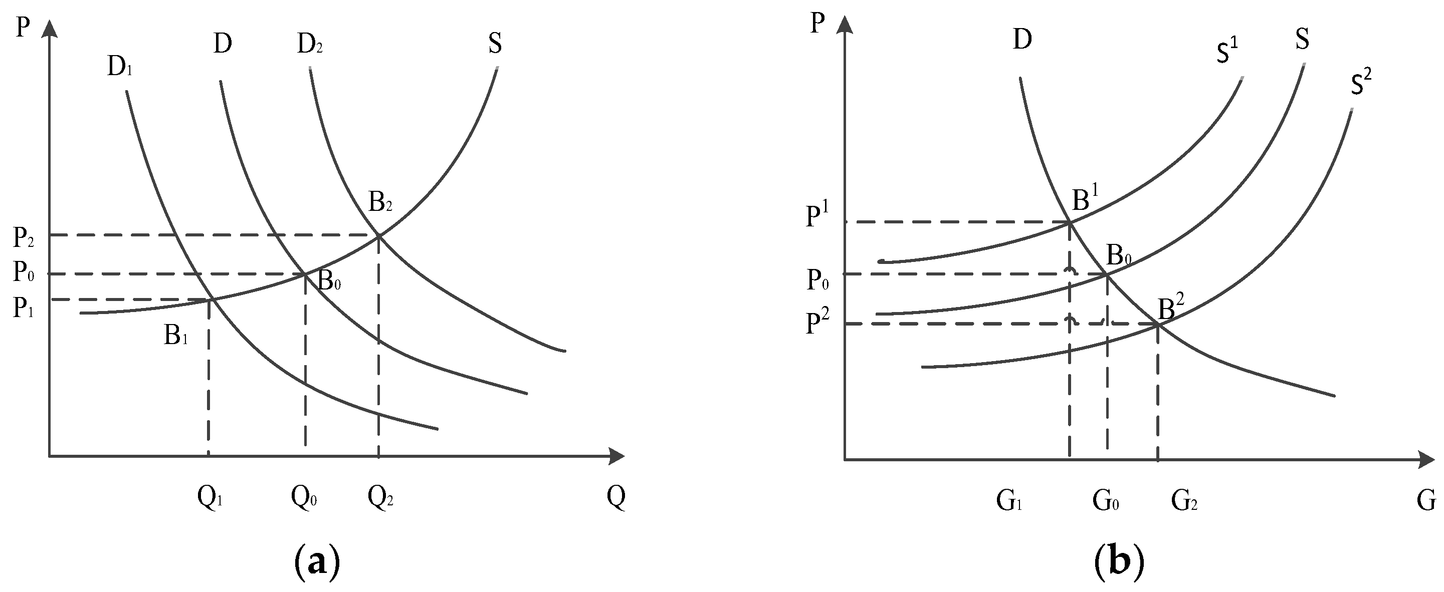
3.2. Elastic Passenger Demand and Choice Behavior

Generalized travel cost is the most critical influencer of passenger demand. It is described by the ticket price and the travel time (Deng et al. [27]):

$$c_{lrs}^k=p_{lrs}^k+\nu ·t_{lrs}$$

(2)

where $t_{lrs}$ is the travel time of train $l$ on OD $\left(r,s\right)$ in pre-sale period $k$, and $\nu$ is the time value conversion coefficient.

Then, the average generalized travel cost of $\left(r,s\right)$ is

$${\mathrm{c}}_{rs}^k=\frac{1}{{{\displaystyle \sum }}_{l\in L}{x}_l^r·x_l^s}{\displaystyle \sum }_{l\in L}{\displaystyle \sum }_{k=1}^K{c}_{lrs}^k·x_l^r·x_l^s$$

(3)

The passenger flow demand will vary flexibly with the generalized travel cost. Here, the log-linear function is used (Qi et al. [35]) to describe the elastic demand of $\left(r,s\right)$ in period $k$.

$$q_{rs}^k\left({\mathrm{c}}_{rs}^k\right)=q_{rs}^{k0}\left({\mathrm{c}}_{rs}^{k0}\right)\cdot \exp \left[-{\eta }^k\left(\frac{c_{rs}^k}{c_{rs}^{k0}}-1\right)\right]$$

(4)

where $c_{rs}^{k0}$ is the average generalized travel cost of $\left(r,s\right)$ under the fixed pricing strategy, $q_{rs}^{k0}\left({\mathrm{c}}_{rs}^{k0}\right)$ is the corresponding passenger demand, and ${\eta }^k$ is the elastic demand function coefficient in pre-sale period $k$.

For all trains that can serve $\left(r,s\right)$, we use the logit model to describe passengers’ choice behavior among them (Qin et al. [26]):

$${\phi }_{lrs}^k=\frac{\exp \left(-\theta c_{lrs}^k\right)}{{\sum }_{l^{\prime }\in L}\exp \left(-\theta c_{l^{\prime }rs}^k\right)}$$

(5)

where $\theta$ is the utility conversion coefficient.

Then, the elastic passenger demand of train $l$ on $\left(r,s\right)$ in pre-sale period $k$ can be obtained by

$$q_{lrs}^k=q_{rs}^k\left({\mathrm{c}}_{rs}^k\right)\cdot {\phi }_{lrs}^k=q_{rs}^{k0}\left({\mathrm{c}}_{rs}^{k0}\right)\cdot \exp \left[-{\eta }^k\left(\frac{{\mathrm{c}}_{rs}^k}{{\mathrm{c}}_{rs}^{k0}}-1\right)\right]\cdot \frac{\exp \left(-\theta c_{lrs}^k\right)}{{\sum }_{l^{\prime }\in L}\exp \left(-\theta c_{l^{\prime }rs}^k\right)}$$

(6)

3.3. Integrated Optimization Model of Ticket Pricing and Stop Planning

3.3.1. Objective Function

In order to improve the revenue of the enterprise, the objective function is constructed based on two aspects: maximizing the transport revenue for HSR and minimizing the total time loss for passengers.

(1)

Transport revenue

The revenue is the difference between the ticket income and the stopping cost of all trains.

$$R={\displaystyle \sum }_{k=1}^K{\displaystyle \sum }_{\left(r,s\right)\in W}{\displaystyle \sum }_{l\in L}{y}_{lrs}^k·p_{lrs}·z_{lrs}^k-{\displaystyle \sum }_{l\in L}{\displaystyle \sum }_{n=2}^{N-1}{x}_l^n·{\pi }_l^n$$

(7)

where $z_{lrs}^k$ is the number of seats that train $l$ allocates to $\left(r,s\right)$ in pre-sale period $k$, $x_l^n$ is the stopping variable, and ${\pi }_l^n$ is the stopping cost of train $l$ at station $n$.

(2)

Time loss of passengers

The time loss of passengers is determined by trains’ stopping time at each intermediate station. We introduce passengers’ average unit time value $\partial$ to describe it.

$$\mathrm{V}=\nu ·{\displaystyle \sum }_{\left(r,s\right)\in W}{\displaystyle \sum }_{l\in L}\left[{\displaystyle \sum }_{k=1}^K{z}_{lrs}^k·{\displaystyle \sum }_{n=r+1}^{s-1}{x}_l^n{u}_l^n\right]$$

(8)

where $u_l^n$ is the stopping time of train $l$ at station $n$.

Finally, use weighting coefficients ${\omega }_1$ and ${\omega }_2$ to unify the sub-objective functions as a single objective function

$$\max Z={\omega }_1·R-{\omega }_2·V$$

(9)

where ${\omega }_1$ and ${\omega }_2$ should be determined according to the importance of each sub-objective function. Here, the values of ${\omega }_1$ and ${\omega }_2$ are, respectively, taken as 0.6 and 0.4.

3.3.2. Constraints

(1)

Price constraints

At first, the ticket price must be positive.

$$y_{lrs}^k>0 \left(r,s\right)\in \mathit{W},l\in \mathit{L},1\le k\le K$$

(10)

For the railway enterprises to better organize passenger transport, it is necessary to prevent passengers from buying tickets near the departure time. Thus, the closer to the departure time, the higher the ticket price should be.

$$y_{lrs}^{k-1}\le y_{lrs}^k \left(r,s\right)\in \mathit{W},l\in \mathit{L},2\le k\le K$$

(11)

(2)

Ticket (seat) constraints

Firstly, the number of tickets that any train $l$ allocates to $\left(r,s\right)$ in period $k$ should be an integer.

$$z_{lrs}^k\in N \left(r,s\right)\in \mathit{W},l\in \mathit{L},1\le k\le K$$

(12)

Secondly, a train may allocate tickets to OD $\left(r,s\right)$ only when it can serve the OD.

$$\left(x_l^r·x_l^s-1\right)·z_{lrs}^k=0 \left(r,s\right)\in \mathit{W},l\in \mathit{L},1\le k\le K$$

(13)

Finally, the number of tickets (seats) that train $l$ allocates to $\left(r,s\right)$ in period $k$ should not exceed the passenger demand (Deng et al. [27]).

$$z_{lrs}^k\le q_{lrs}^k+r_{lrs}^{\to k} \left(r,s\right)\in \mathit{W},l\in \mathit{L},1\le k\le K$$

(14)

where $r_{lrs}^{\to k}$ refers to the passenger demand that is rejected in pre-sale period $k$ − 1 and continues to choose train $l$ in period $k$. The setting of this variable makes it possible for the passenger demand rejected in early periods to be satisfied in subsequent periods, so that more passenger demand can be satisfied. According to the assumption (3), passengers who fail to obtain tickets in a certain period will continue to buy tickets in the next period. The transfer passenger demand can be regarded as part of the initial passenger flow in the next period. Therefore, if the rejected passenger demand is denoted as $f_{rs}^{k-1}$, $r_{lrs}^{\to k}$ can be obtained according to:

$$r_{lrs}^{\to k}=f_{rs}^{k-1}\cdot {\phi }_{lrs}^k=f_{rs}^{k-1}\cdot \exp \left[-{\eta }^k\left(\frac{{\mathrm{c}}_{rs}^k}{{\mathrm{c}}_{rs}^{k0}}-1\right)\right]\cdot \frac{\exp \left(-\theta c_{lrs}^k\right)}{{{\displaystyle \sum }}_{l^{\prime }\in L}\exp \left(-\theta c_{l^{\prime }rs}^k\right)}$$

(15)

(3)

Capacity constraints

The number of tickets allocated by a train to any section cannot exceed the train’s capacity.

$${\displaystyle \sum }_{k=1}^K{\displaystyle \sum }_{r=1}^j{\displaystyle \sum }_{s=j+1}^N{z}_{lrs}^k\le C_l l\in \mathit{L},\forall j\in \left[1,N-1\right]$$

(16)

where $C_l$ is the carrying capacity of train $l$.

(4)

Reachability constraints

For each OD pair, there must be trains that can serve it.

$${\displaystyle \sum }_{l\in L}{x}_l^r·x_l^s\ge 1 \left(r,s\right)\in \mathit{W}$$

(17)

To sum up the above expressions (1)–(17), Equations (2), (4), (5), and constraint (14) refer to existing studies, while others are newly proposed here.

The objective function (9), Constraint (13), Constraint (15), and Constraint (17) are nonlinear, while other constraints are linear. Constraint (13) can be linearized by introducing a large enough positive number $\mathit{M}$:

$${\mathit{z}}_{\mathit{l}\mathit{r}\mathit{s}}^{\mathit{k}}\le \mathit{M}\mathit{·}{\mathit{x}}_{\mathit{l}}^{\mathit{r}} \left(\mathit{r},\mathit{s}\right)\in \mathit{W},\mathit{l}\in \mathit{L},\mathit{1}\le \mathit{k}\le \mathit{K}$$

(18)

$${\mathit{z}}_{\mathit{l}\mathit{r}\mathit{s}}^{\mathit{k}}\le \mathit{M}·{\mathit{x}}_{\mathit{l}}^{\mathit{s}} \left(\mathit{r},\mathit{s}\right)\in \mathit{W},\mathit{l}\in \mathit{L},\mathit{1}\le \mathit{k}\le \mathit{K}$$

(19)

Constraint (17) can be linearized by introducing a new binary variable $g_{lrs}$:

$${\displaystyle \mathit{\sum }}_{\mathit{l}\in \mathit{L}}{\mathit{g}}_{\mathit{l}\mathit{r}\mathit{s}}\ge \mathit{1} \left(\mathit{r},\mathit{s}\right)\in \mathit{W}$$

(20)

$${\mathit{g}}_{\mathit{l}\mathit{r}\mathit{s}}\le {\mathit{x}}_{\mathit{l}}^{\mathit{r}} \left(\mathit{r},\mathit{s}\right)\in \mathit{W},\mathit{l}\in \mathit{L}$$

(21)

$${\mathit{g}}_{\mathit{l}\mathit{r}\mathit{s}}\le {\mathit{x}}_{\mathit{l}}^{\mathit{s}} \left(\mathit{r},\mathit{s}\right)\in \mathit{W},\mathit{l}\in \mathit{L}$$

(22)

Finally, the joint optimization model for HSR ticket pricing and train stop planning can be formulated as follows s.t.

$$\mathit{max}Z={\omega }_1·R-{\omega }_2·V$$

(23)

Constraints (10)–(12), (14)–(16), and (18)–(22)

Table 4. Characteristics of the formulated model.

Item	Type	Size	Characteristic
$y_{lrs}^k$	Variable	$\left(\left|\mathit{L}\right|·N\left(N-1\right)·\right)⁄2$	Discrete
$x_l^n$	Variable	$\left|\mathit{L}\right|·\left(N-2\right)$	Binary
$z_{lrs}^k$	Variable	$\left(\left|\mathit{L}\right|·N\left(N-1\right)·K\right)⁄2$	Integer
$g_{lrs}$	Variable	$\left(\left|\mathit{L}\right|·N\left(N-1\right)\right)⁄2$	Binary
Constraint (10)	Constraint	$\left(\left|\mathit{L}\right|·N\left(N-1\right)·K\right)⁄2$	Linear
Constraint (11)	Constraint	$\left(\left|\mathit{L}\right|·N\left(N-1\right)·\left(K-1\right)\right)⁄2$	Linear
Constraint (12)	Constraint	$\left(\left|\mathit{L}\right|·N\left(N-1\right)·K\right)⁄2$	Linear
Constraint (14)	Constraint	$\left(\left|\mathit{L}\right|·N\left(N-1\right)·K\right)⁄2$	Linear
Constraint (15)	Constraint	$\left(\left|\mathit{L}\right|·N\left(N-1\right)·\left(K-1\right)\right)⁄2$	Nonlinear
Constraint (16)	Constraint	$\left|\mathit{L}\right|·\left(N-1\right)$	Linear
Constraint (18)	Constraint	$\left(\left|\mathit{L}\right|·N\left(N-1\right)·K\right)⁄2$	Linear
Constraint (19)	Constraint	$\left(\left|\mathit{L}\right|·N\left(N-1\right)·K\right)⁄2$	Linear
Constraint (20)	Constraint	$\left(N\left(N-1\right)\right)⁄2$	Linear
Constraint (21)	Constraint	$\left(\left|\mathit{L}\right|·N\left(N-1\right)\right)⁄2$	Linear
Constraint (22)	Constraint	$\left(\left|\mathit{L}\right|·N\left(N-1\right)\right)⁄2$	Linear

details the variables and constraints in the formulated model.

4. Solution Method

As an HSR line usually has many intermediate stations and an HSR train has many seats, the model proposed above is a super-large-scale mixed-integer nonlinear programming model. Numerous variables and constraints make it difficult to solve the model with efficient and accurate algorithms. Thus, a heuristic algorithm is chosen for solving and computational analysis. Moreover, the joint problem is a combinatorial optimization problem, which has a strong similarity with the solid annealing principle of SA (as shown in

Table 5. Solid annealing vs. combinatorial optimization.

Solid Annealing	Combinatorial Optimization
State	Solution
System energy	The objective function
The lowest energy state	The optimal solution
Heating to melt	Setting the initial temperature
Isothermal process	Generating and accepting (or rejecting) new solutions
Cooling process	Changing the current temperature

). Thus, we will design an efficient method based on SA to solve the joint model.

The simulated annealing (SA) algorithm is a stochastic algorithm based on Monte-Carlo iteration, which involves asymptotic convergence and allows random movements in the searched neighborhood to escape local minima. It randomly searches for the global optimal solution in the solution collection, and can jump out with a certain probability when falling into the local optimum. In addition, it is easy to implement and less limited by the initial solution. Although proposed more than 40 years ago, it still attracts some attention and is broadly used in many existing solutions for different variants of optimization problems.

HSR’s dynamic pricing, seat allocation scheme, and stop plan are mutually influential and restrictive. Once obtained, the optimal stop plan remains unchanged in the pre-sale period. However, the ticket price and seats allocated for the same OD pair are different for each period. Thus, the optimization process can be divided into two layers. The stop plan is first optimized in the outer layer, and then the ticket price and seat allocation scheme under the determined stop plan are optimized in the inner layer level. Thus, the CSA algorithm is proposed for solving the problem. In this way, the algorithm only needs to search for the optimal solution in a smaller solution space in each iteration, so that improves the possibility of searching for the global optimum in the same computing time. If an appropriate termination strategy is adopted, the algorithm can effectively save computing time.

The CSA algorithm needs to start the iterative process based on the initial solution. For our problem, the initial solution includes three aspects: the initial stop plan, ticket prices, and seat allocation scheme. We set them according to the current operational mode of HSR.

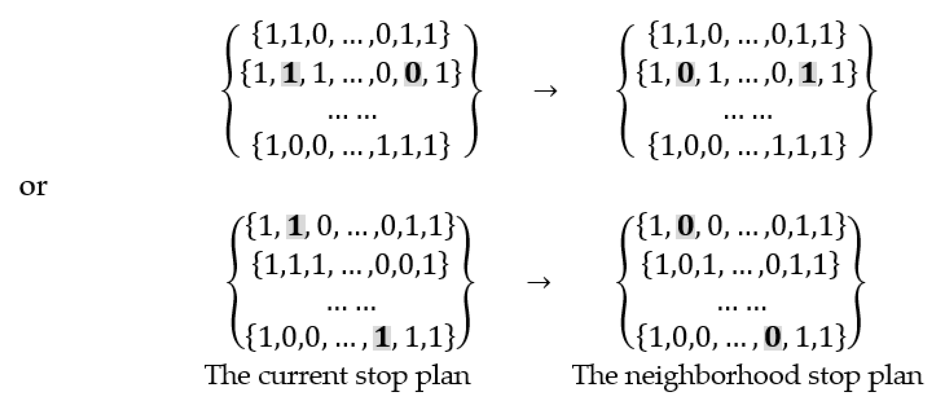
4.1. Neighborhood Structure

The neighborhood of the CSA algorithm is divided into inner and outer layers to be constructed separately.

4.1.1. Outer Neighborhood

The outer layer optimizes the stop plan. The stop mode of a train is described by a vector composed of the 0–1 variable, in which 1 indicates stopping at the station and 0 indicates no stopping.

As shown in Figure 3, the neighborhood structure of the outer layer can be constructed in two ways. One involves randomly selecting two intermediate stopping variables of one train for inversion. Another involves randomly selecting two trains, and inverting one intermediate stopping variable of each train. If the newly obtained stop plan does not satisfy the OD pair reachability constraint, we return to the reconstruction.

4.1.2. Inner Neighborhood

The inner layer determines the ticket price and seat allocation. We randomly select a coefficient $y_{lrs}^k$ from the current price discount solution and ${\beta }^{\prime }$ from the set $\left\{{\beta }_i\in \mathit{\beta }|y_{lrs}^{k-1}\le {\beta }_i\le y_{lrs}^{k+1}\right\}$. Then let $y_{lrs}^k\leftarrow {\beta }^{\prime }$ to construct the neighborhood ticket price solution.

Under the new stop plan and ticket prices, we obtain the passenger demand by Formulas (1)–(6) and round it as the pre-seat allocation scheme. If it satisfies all constraints, the scheme is regarded as a new feasible seat allocation scheme. If any constraints are not satisfied, corresponding adjustments are required. For any train $l^{\prime }$ and any section $\left(j^{\prime },j^{\prime }+1\right)$ that exceed the train capacity limit (constraints (16)), we adjust the pre-seat allocation scheme to obtain a feasible scheme.

$$z_{l^{\prime }rs}^k=\frac{q_{l^{\prime }rs}^k}{{{\displaystyle \sum }}_{k=1}^K{{\displaystyle \sum }}_{r=1}^{j^{\prime }}{{\displaystyle \sum }}_{s=j^{\prime }+1}^N{q}_{l^{\prime }rs}^k}\times C_{l^{\prime }} l^{\prime }\in L,r\le j^{\prime }<j^{\prime }+1\le s,1\le k\le K$$

(24)

4.2. Implementation Process

In the CSA, the initial temperature is given by the objective function value of the initial feasible solution, the temperature drops proportionally with a given cooling parameter, and the number of iterations under the same temperature is controlled by an upper limit. When the current temperature is lower than the given end temperature or the current best solution remains unchanged within the specified number of iterations, the algorithm is terminated.

The steps of the CSA algorithm are as follows.

Step 1: Initialization. Set the initial temperature $T_0$, the cooling parameter $\alpha$, the end temperature $T_{min}$, and the maximum iteration numbers $I_1$ and $I_2$ for the inner and outer layer algorithms under the same temperature. Determine the initial feasible solution $\mathit{S}$ and calculate the objective function value Z($\mathit{S}$). Let the current temperature $t=T_0$, and the current iteration number $i=i^{\prime }=1$. The best solution $\overline{\mathit{S}}=\mathit{S}$.

Step 2: Construction of the outer neighborhood solution. Implement the outer neighborhood structure method to obtain a new train stop plan.

Step 3: Perform the inner algorithm.

Step 3.1: Obtain the initial solution of the inner layer. Under the new stop plan, use the inner neighborhood construction method to obtain a new pricing strategy and seat allocation scheme; that is, a new feasible solution ${\mathit{S}}^{\prime }$. Then, calculate the objective function value $Z\left({\mathit{S}}^{\prime }\right)$.

Step 3.2: Construction of the inner neighborhood solution. Based on the feasible solution ${\mathit{S}}^{\prime }$, implement the inner neighborhood method to obtain a new pricing strategy and seat allocation scheme, which constitutes a new feasible solution ${\mathit{S}}^{″}$. Then, calculate the objective function value $Z\left({\mathit{S}}^{″}\right)$.

Step 3.3: Metropolis criterion test for the inner layer. If $Z\left({\mathit{S}}^{″}\right)\ge Z\left({\mathit{S}}^{\prime }\right)$, let ${\mathit{S}}^{\prime }={\mathit{S}}^{″}$. Otherwise, randomly generate a number $\rho$ from the interval (0,1), and if $\rho \le exp\left(-\raisebox{1ex}{$\left(Z\left({\mathit{S}}^{\prime }\right)-Z\left({\mathit{S}}^{″}\right)\right)$}\!\left/ \!\raisebox{-1ex}{$t$}\right.\right)$, let ${\mathit{S}}^{\prime }={\mathit{S}}^{″}$, otherwise, refuse the inferior solution and keep the current solution ${\mathit{S}}^{\prime }$ unchanged.

Step 3.4: Iteration times test for the inner layer. Let $i^{\prime }\leftarrow i^{\prime }+1$. If $i^{\prime }\ge I_1$, set $i^{\prime }=1$, output the solution ${\mathit{S}}^{\prime },$ and go to step 4; otherwise go to step 3.2.

Step 4: Metropolis criterion test for the outer layer. If $Z\left({\mathit{S}}^{\prime }\right)\ge Z\left(\mathit{S}\right)$, let $\overline{\mathit{S}}={\mathit{S}}^{\prime }$, $\mathit{S}={\mathit{S}}^{\prime }$. Otherwise, randomly generate a number $\rho$ from the interval (0,1), and if $\rho \le exp\left(-\raisebox{1ex}{$\left(Z\left(\mathit{S}\right)-Z\left({\mathit{S}}^{\prime }\right)\right)$}\!\left/ \!\raisebox{-1ex}{$t$}\right.\right)$, let $\mathit{S}={\mathit{S}}^{\text{′}}$, otherwise, refuse the inferior solution and keep the current solution unchanged.

Step 5: Iteration number test for the outer layer. Update the iteration times: $i\leftarrow i+1$. If $i\ge I_2$, let $t\leftarrow t·\alpha$, $i=1,$ and go to step 6; otherwise go to step 2.

Step 6: Termination check. If $t<T_{min}$ or the current optimal solution $\overline{\mathit{S}}$ remains unchanged in $\tau$ iterations, terminate the algorithm and output the optimal solution $\overline{\mathit{S}}$; otherwise, reset $i=1$ and go to step 2.

It should be noted that the CSA algorithm records the best solution $\overline{\mathit{S}}$. Once a better solution is found, the algorithm will replace $\overline{\mathit{S}}$ with the better one regardless of the Metropolis criterion. Thus, the utilization efficiency of the searched optimal solution can be improved significantly.

5. Empirical Analysis

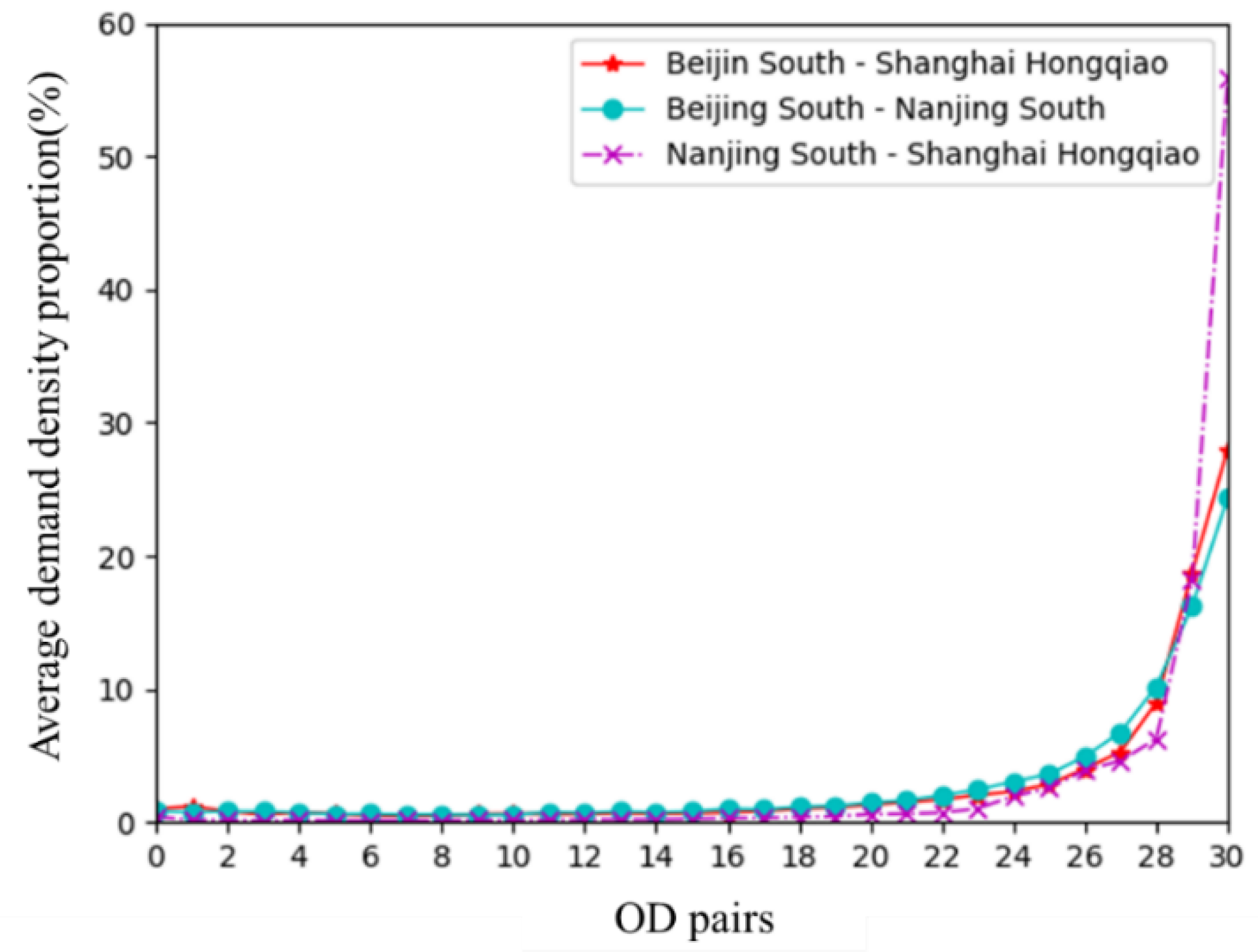
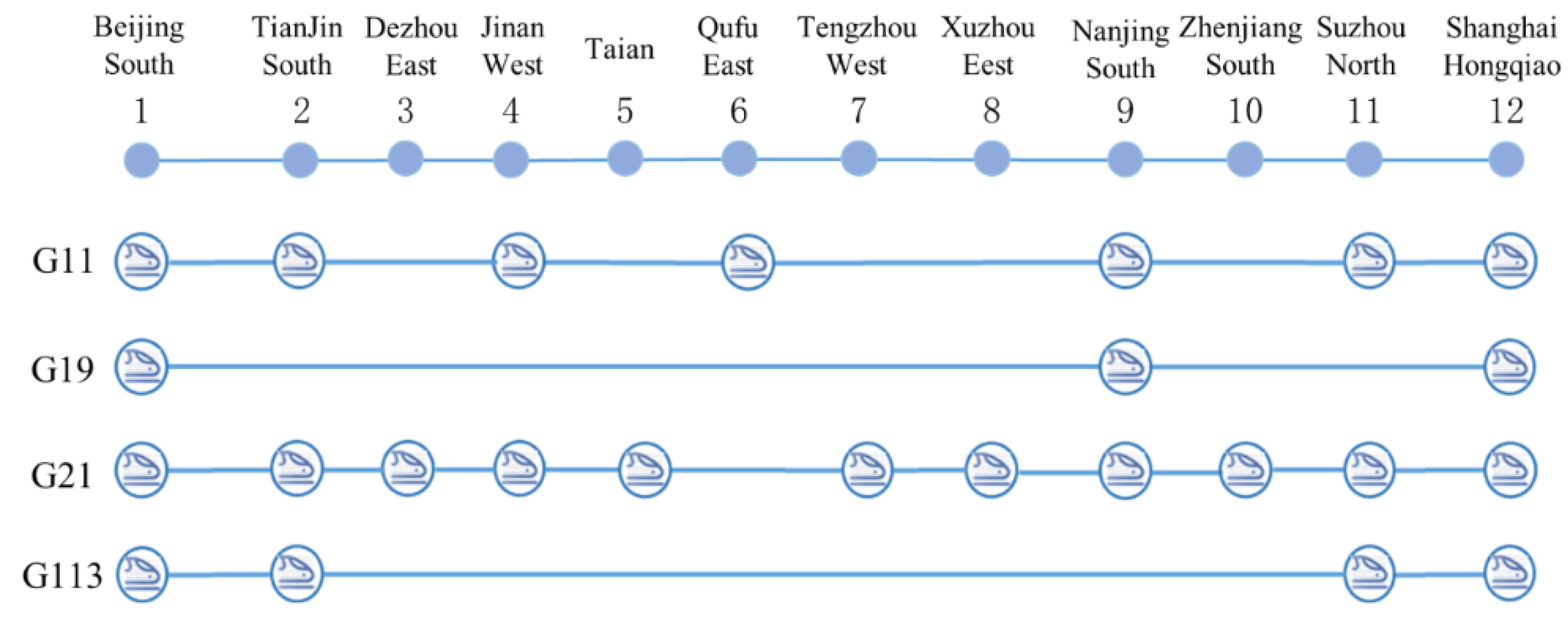
5.1. Basic Data

The Beijing–Shanghai HSR line is taken as an example to verify the feasibility of the model and algorithm. Among the trains that depart from Beijing South Station and arrive at Shanghai Hongqiao station, four trains G11, G19, G21, and G113 with different stopping patterns are selected for analysis. As Figure 4 shows, these four trains involve 12 stations: Beijing South, Tianjin South, Dezhou East, Jinan West, Taian, Qufu East, Tengzhou East, Xuzhou West, Nanjing South, Zhenjiang South, Suzhou North, and Shanghai Hongqiao. We number them 1–12 sequentially, where 1 and 12 represent Beijing South and Shanghai Hongqiao, respectively. To simplify the problem, we suppose that all HSR transport services adopt the same price discount in the same pre-sale period.

Each train is formed of 16 cars, and its stopping cost and stopping time at each station are 3200 yuan and 7 min, respectively. The seat number of G11, G21, and G113 is 1043, while that of G19 is 1015.

According to the ticket data from 1 August 2016 to 31 July 2017, we can depict passengers’ booking rules in Figure 5 and further divide the ticket pre-sale period into four periods: pre-sale days 1–19, 20–25, 26–28, and 29–30. The elastic demand function coefficient ${\eta }^k$ reflects the sensitivity of passenger demand to ticket prices, which intensifies as the departure date approaches. We take ${\eta }^k$ as 1.8, 1.4, 1.2, and 0.8 for periods 1–4, respectively.

The highest (corresponding to the published price) and lowest price discounts are 1 and 0.56, respectively, and we take the interval of 0.04 to define the price discount coefficient set $\mathit{\beta }=\left\{0.56, 0.60, \dots , 0.96, 1\right\}$. According to Qi et al. [35], we have $\nu =0.6$ yuan/minute and $\theta$ = 0.012. For the CSA algorithm, $I_1=7920$, $I_2=400$, $\alpha =0.95$, $T_{min}=0.001$, and $\tau =100$.

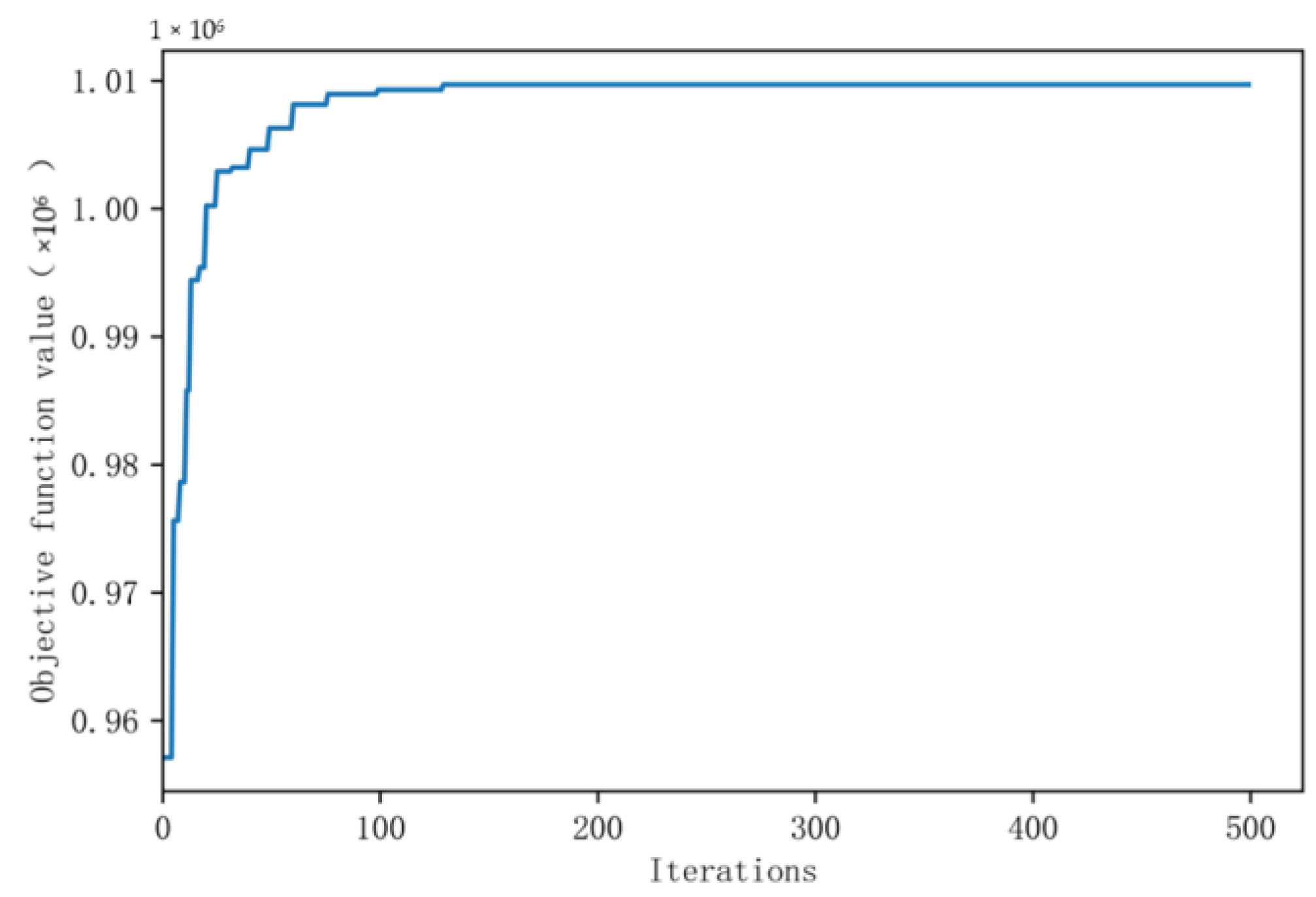
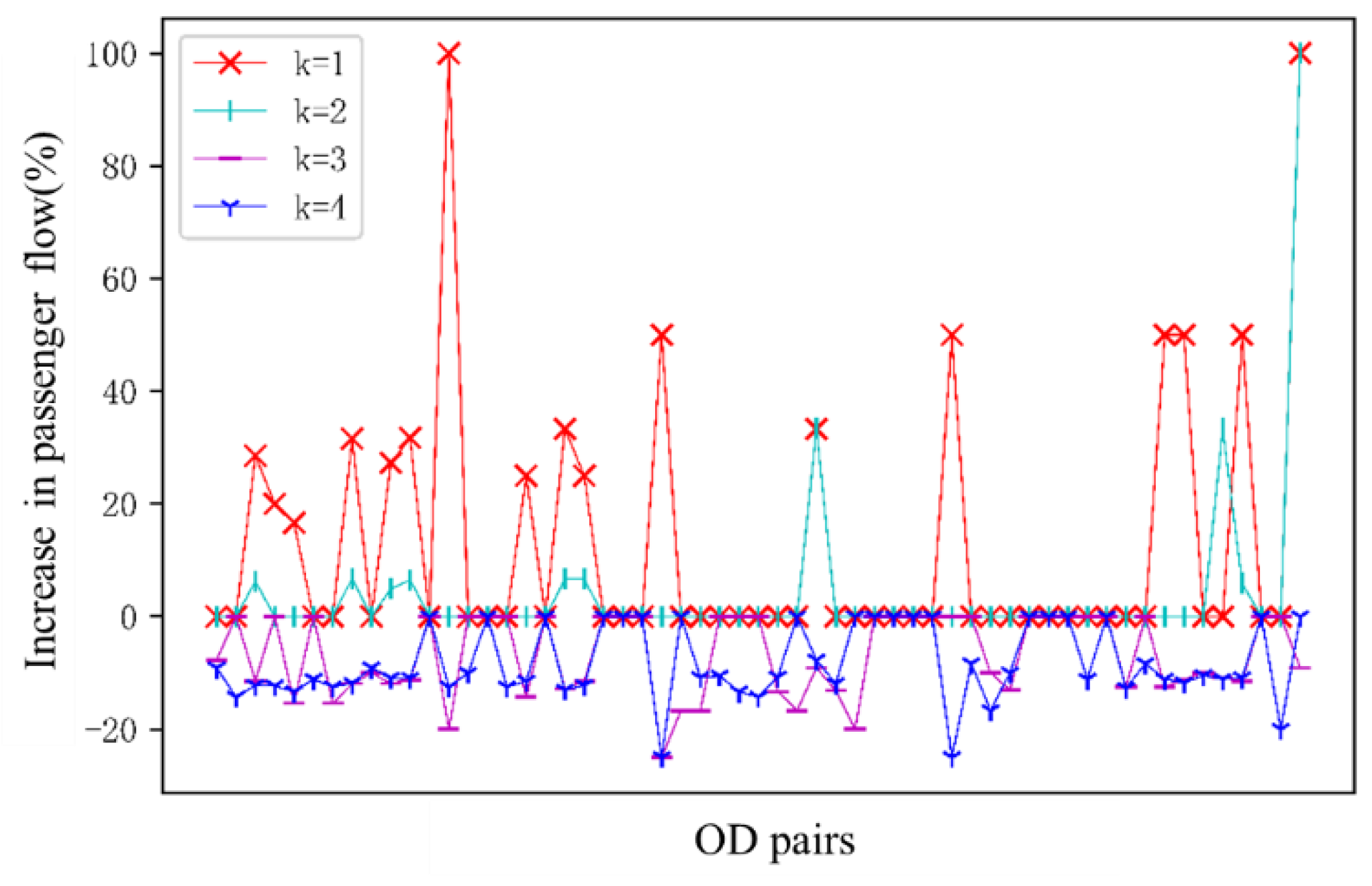
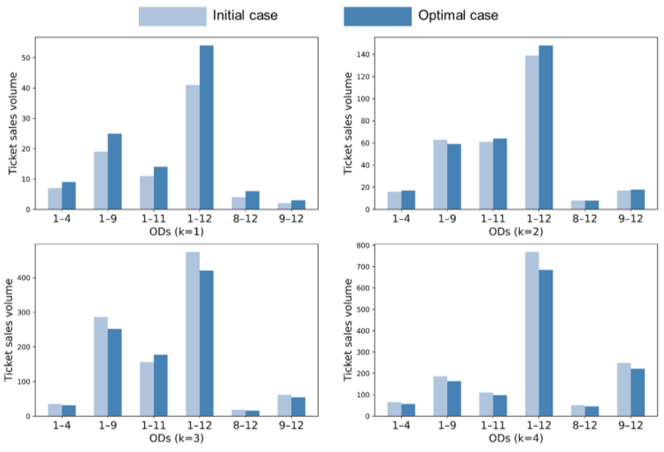
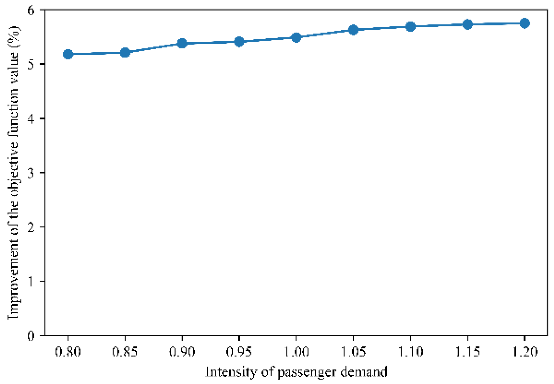
5.2. Results and Analysis

We used the Python programming language to implement the algorithm and solve the model. Figure 6 presents the iteration process of the CSA algorithm. The objective value starts to converge around 130 iterations and remains unchanged thereafter.

The results show that the transportation revenue and the total passenger time loss are 1,717,166 yuan and 85,829 min, respectively. Compared with 1,633,840 yuan and 96,600 min under the current fixed operational mode, the revenue increased by 5.10% and the time loss decreased by 11.15%.

Figure 7 shows the optimal stop plan. Compared to the current stop plan shown in Figure 4, the stop frequency is reduced from 22 to 17, and the total stopping cost is reduced by 16,000 yuan (a decrease of 22.73%). G19 and G113 reduced by three and four stops, while G11 and G21 added stops at Station 2 and Station 3, respectively. For some ODs, it indicated that their passenger demand does not necessitate so many trains to serve them. One additional stop for G11 and G21 trains can help meet the demands of these ODs. Moreover, for passengers taking G11 and G21 trains, their stopping time loss only increased by one-stop time, which is less than the reductions in the stopping time loss for passengers on G19 and G113.

Under the fixed operational mode, the passenger flows of G11, G19, G21, and G113 are 1157, 1002, 1113, and 1239, respectively. After optimization, the passenger flows of G11 and G21 increase to 1334 and 1441, while those of G19 and G113 decrease to 705 and 780, respectively. The reason is that G11 and G21 can serve more OD pairs. Conversely, as G19 and G113 reduce stops at several intermediate stations, they no longer serve part of the OD pairs. As a result, the passenger flow of these OD pairs transfers to G11 and G21.

Table 6. Ticket prices for different ticket pre-sale periods.

OD Pairs	Dynamic Prices (Yuan)				Public Prices (Yuan)	Current Prices (Yuan)
	$\mathit{k}$ = 1	$\mathit{k}$ = 2	$\mathit{k}$ = 3	$\mathit{k}$ = 4
1–4	129	175.5	203	221.5	230.5	184.5
1–9	310.5	421.5	488	532	554.5	443.5
1–11	366.5	497.5	576	628	654.5	523.5
1–12	387	525.5	608.5	663.5	691	553.0
8–12	195.5	265	307	335	349	279.0
9–12	94	128	148	161.5	168	134.5

gives the optimal dynamic pricing strategy for some ODs (the ticket price is accurate to 0.5 yuan). For any OD, the closer the period is to the departure date, the higher the ticket price. The dynamic price is lower than the fixed price for the first two periods, while it is higher for the last two periods. This is because passengers are generally more sensitive to the ticket price during early ticket pre-sale time, so the passenger demand is rich in elasticity. Discounts on ticket prices in early periods can attract more passengers to buy tickets.

As shown in Figure 8, the passenger flow of most ODs has increased significantly in the first period. By exchanging low ticket prices for more passengers, the revenue can be enhanced. However, passengers booking tickets in the last two periods usually make their travel plans temporarily. Most of them are less sensitive to price and more willing to accept higher ticket prices. Thus, raising ticket prices hardly affects their demand. It can be seen from Figure 8 that the passenger flow of most ODs falls by less than 15% for the last two periods. The contribution of raising the price is more significant than the loss of passenger flow, which can also expand the revenue.

Figure 9 compares the ticket sales under the fixed price (initial case) and dynamic price (optimal case). The closer the period is to the departure date, the higher the ticket sale volume. For all ODs, the tickets are sold in the latter two periods, which matches the distribution of passenger demand and thus is conducive to obtaining more ticket revenue.

Compared to the fixed price, the ticket sales volume of most ODs in the first two periods increased significantly, which indicates that the dynamic pricing strategy can effectively guide passengers to purchase tickets earlier, which is beneficial for railway enterprises to organize passenger transport.

Table 7. Passenger flow of each OD pair (before/after optimization).

1	2	3	4	5	6	7	8	9	10	11	12
1	57/63	10/9	189/174	79/74	53/55	9/11	58/53	550/521	33/29	359/345	1422/1334
2		5/5	22/20	13/15	-	3/3	12/12	50/46	7/7	86/87	140/137
3			5/5	-	-	-	3/3	0/0	-	10/10	12/11
4				43/38	21/23	16/14	22/19	53/48	11/12	30/28	110/97
5					-	9/10	0/0	5/5	0/0	0/0	11/14
6						-	-	15/10	0/0	16/19	42/45
7							1/1	/0	/0	9/8	/0
8								83/74	14/17	49/45	81/75
9									59/65	139/126	329/299
10										2/2	9/8
11											145/129

gives the passenger flow comparison of each OD before and after optimization. The optimized passenger flow of some ODs increased, but that of more ODs decreased slightly. For most ODs, passengers prefer to buy tickets in the last two periods. The rise in ticket prices will cause some passengers to give up HSR and choose another transport mode. In addition, the passenger demand for the first two periods is relatively weak. Although the ticket price is discounted, only a small number of passengers were attracted. Thus, the passenger flow of most ODs decreased overall.

Although the total stopping frequency of all trains decreased, the passenger flow of each OD hardly fluctuates. The underlined data in Table 7 denotes the OD whose service frequency is reduced. We can see that the passenger flow fluctuation of these ODs (13.64~1.16%) is not greater than that of other ODs (−33.33~27.27%). This indicates that our model can reasonably adjust the stop plan according to the dynamic passenger demand, which can reduce the stopping cost while maintaining passenger flows and ensuring service quality.

Figure 10 shows the improvement of the objective function value (OFV) under different passenger demands, which indicates that our method can always effectively improve the quality of the optimal combinatorial scheme. The OFV is growing with increases in passenger demand. But after the demand reaches a certain level, the growth rate of the OFV gradually slows as the demand continuously increases. This is because after the total demand has exceeded the transport capacity of the HSR system, the ticket prices for later pre-sale periods will reach the ceiling price. Then, when the demand continues to increase, the highest prices should remain unchanged, which results in the reduction of the OFV’s growth rate.

6. Conclusions

In this paper, we introduced a mixed-integer non-linear model for jointly optimizing HSR ticket pricing and train stop planning considering multiple trains with multiple stopping patterns, and proposed a CSA algorithm combining the characteristics of the problem. The objective was to maximize the revenue of railway enterprises and minimize the total travel time of passengers. An empirical study based on ticket reservation data was conducted to present the performance of the proposed model and algorithm.

The results obtained illustrate the impacts that the strategy derived from the optimization model has on passenger demand, capacity allocation, and revenue. The solution from the proposed method provides a significant improvement in revenue from the initial 5.1% and causes a marked decline in the total travel time loss of passengers from the initial 11.5%. The dynamic pricing strategy encourages more passengers to buy tickets in earlier pre-sale periods. The optimized train stop plan decreases the total stopping cost of railway enterprises and the total time loss of passengers. In conclusion, this paper has illustrated how railway operators can exploit existing data sources to further realize RM.

The following areas indicate possible directions for future research. Other factors should be considered in the railway RM problem, such as seat classes and ticket cancellations. It would also be interesting to develop a more efficient algorithm that combines exact and metaheuristic methods to solve the proposed model.

References

1. Weatherford, L.R.; Kimes, S.E. A comparison of forecasting methods for hotel revenue management. Int. J. Forecast. 2003, 19, 401–415. [Google Scholar] [CrossRef] [Green Version]
2. Noone, B.M.; Mattila, A.S. Hotel revenue management and the internet: The effect of price presentation strategies on customers’ willingness to book. Int. J. Hosp. Manag. 2009, 28, 272–279. [Google Scholar] [CrossRef]
3. Heo, C.Y.; Lee, S. Influences of consumer characteristics on fairness perceptions of revenue management pricing in the hotel industry. Int. J. Hosp. Manag. 2011, 30, 243–251. [Google Scholar] [CrossRef]
4. Grauberger, W.; Kimms, A. Airline revenue management games with simultaneous price and quantity competition. Comput. Oper. Res. 2016, 75, 64–75. [Google Scholar] [CrossRef]
5. Lawhead, R.J.; Gosavi, A. A Bounded Actor-Critic Reinforcement Learning Algorithm Applied to Airline Revenue Management. Eng. Appl. Artif. Intell. 2019, 82, 252–262. [Google Scholar] [CrossRef]
6. Selcuk, A.M.; Avar, Z.M. Dynamic pricing in airline revenue management. J. Math. Anal. Appl. 2019, 478, 1191–1217. [Google Scholar] [CrossRef]
7. Kyparisis, G.J.; Koulamas, C. Optimal pricing and seat allocation for a two-cabin airline revenue management problem. Int. J. Prod. Econ. 2018, 201, 18–25. [Google Scholar] [CrossRef]
8. Armstrong, A.; Meissner, J. Railway Revenue Management: Overview and Models; Lancaster University Management School: Lancaster, UK, 2010. [Google Scholar]
9. Abe, I. Revenue Management in the Railway Industry in Japan and Portugal: A Stakeholder Approach. Technology and Policy Program. Ph.D. Thesis, Massachusetts Institute of Technology, Cambridge, MA, USA, 2007. [Google Scholar]
10. Bharill, R.; Rangaraj, N. Revenue management in railway operations: A study of the Rajdhani Express, Indian Railways. Transp. Res. Part A Policy Pract. 2008, 42, 1195–1207. [Google Scholar] [CrossRef]
11. Riss, M.; Côté, J.P.; Savard, G. A new revenue optimization tool for high-speed railway: Finding the right equilibrium between revenue growth and commercial objectives. In Proceedings of the 8th World Congress on Railway Research, Seoul, Korea, 18–22 May 2008. [Google Scholar]
12. Crevier, B.; Cordeau, J.F.; Savard, G. Integrated operations planning and revenue management for rail freight transportation. Transp. Res. Part B Methodol. 2012, 46, 100–119. [Google Scholar] [CrossRef]
13. Vuuren, D.V. Optimal pricing in railway passenger transport: Theory and practice in the Netherlands. Transp. Policy 2002, 9, 95–106. [Google Scholar] [CrossRef]
14. Jarocka, M.; Ryciuk, U. Pricing in the railway transport. In Proceedings of the 9th International Scientific Conference “Business and Management 2016”, Vilnius, Lithuania, 12–13 May 2016. [Google Scholar]
15. Zhang, J.; Yang, X.; Du, G. Research on High-speed Railway Fare Optimization based on Change of Passenger Flow. In Proceedings of the 3rd International Conference on Mechatronics Engineering and Information Technology (ICMEIT 2019), Dalian, China, 29–30 March 2019. [Google Scholar]
16. Dargay, J.M.; Clark, S.; Rose, J. The determinants of long distance travel in Great Britain. Transp. Res. Part A Policy Pract. 2012, 46, 576–587. [Google Scholar] [CrossRef]
17. Georggi, N.L.; Pendyala, R.M. Analysis of long-distance travel behavior of the elderly and the low-income. Transp. Res. Rec. 2012, E-C026, 121–150. [Google Scholar]
18. Sato, K.; Sawaki, K. Dynamic pricing of high-speed rail with transport competition. J. Revenue Pricing Manag. 2011, 11, 548–559. [Google Scholar] [CrossRef]
19. Chen, J.H.; Gao, Z.Y. Optimal Railway Passenger-ticket Pricing. J. China Railw. Soc. 2005, 27, 16–19. [Google Scholar]
20. Wang, X.C.; Wang, H.; Zhang, X.N. Stochastic seat allocation models for passenger rail transportation under customer choice. Transp. Res. Part E 2016, 96, 95–112. [Google Scholar] [CrossRef]
21. Jiang, X.S.; Chen, X.Q.; Zhang, L.; Zhang, R. Dynamic Demand Forecasting and Ticket Assignment for High-Speed Rail Revenue Management in China. Transp. Res. Rec. 2015, 2475, 37–45. [Google Scholar] [CrossRef]
22. Yan, Z.Y.; Li, X.J.; Zhang, Q.; Han, B.M. Seat allocation model for high-speed railway passenger transportation based on flexible train composition. Comput. Ind. Eng. 2020, 142, 106383. [Google Scholar] [CrossRef]
23. Hetrakul, P.; Cirillo, C. A latent class choice based model system for railway optimal pricing and seat allocation. Transp. Res. Part E 2014, 61, 68–83. [Google Scholar] [CrossRef]
24. Hu, X.L.; Shi, F.; Xu, G.M.; Qin, J. Joint optimization of pricing and seat allocation with multiperiod and discriminatory strategies in high-speed rail networks. Comput. Ind. Eng. 2020, 148, 106690. [Google Scholar] [CrossRef]
25. Wu, X.K.; Qin, J.; Qu, W.X.; Zeng, Y.J.; Yang, X. Collaborative Optimization of Dynamic Pricing and Seat Allocation for High-speed Railways: An Empirical Study from China. IEEE Access 2019, 7, 139409–139419. [Google Scholar] [CrossRef]
26. Qin, J.; Zeng, Y.J.; Yang, X.; He, Y.X.; Wu, X.K.; Qu, W.X. Time-Dependent Pricing for High-Speed Railway in China Based on Revenue Management. Sustainability 2019, 11, 4272. [Google Scholar] [CrossRef] [Green Version]
27. Deng, L.B.; Zeng, N.X.; Chen, Y.X.; Xiao, L.W. A divide-and-conquer optimization method for dynamic pricing of high-speed railway based on seat allocation. J. Railw. Sci. Eng. 2019, 16, 2407–2413. [Google Scholar]
28. Vuchic, V.R. Urban Transit; Wiley: Hoboken, NJ, USA, 2005. [Google Scholar]
29. Chang, Y.H.; Ye, C.H.; Shen, C.C. A multi-objective model for passenger train services planning: Application to taiwan’s high-speed rail line. Transp. Res. Part B 2000, 34, 91–106. [Google Scholar] [CrossRef]
30. Bussieck, M.R.; Lindner, T.; Lübbecke, M.E. A fast algorithm for near cost optimal line plans. Math. Methods Oper. Res. 2004, 59, 205–220. [Google Scholar] [CrossRef]
31. Yang, L.X.; Qi, J.G.; Li, S.K.; Gao, Y. Collaborative optimization for train scheduling and train stop planning on high-speed railways. Omega 2016, 64, 57–76. [Google Scholar] [CrossRef]
32. Jin, G.W.; He, S.W.; Li, J.B.; Guo, X.L.; Li, Y.B. An Approach for Train Stop Planning with Variable Train Length and Stop Time of High-speed Rail Under Stochastic Demand. IEEE Access 2019, 7, 129690–129708. [Google Scholar] [CrossRef]
33. Dong, X.L.; Li, D.W.; Yin, Y.H.; Ding, S.X.; Cao, Z.C. Integrated optimization of train stop planning and timetabling for commuter railways with an extended adaptive large neighborhood search metaheuristic approach. Transp. Res. Part C Emerg. Technol. 2020, 117, 102681. [Google Scholar] [CrossRef]
34. Qi, J.G.; Li, S.K.; Gao, Y.; Yang, K.; Liu, P. Joint optimization model for train scheduling and train stop planning with passengers distribution on railway corridors. J. Oper. Res. Soc. 2018, 69, 556–570. [Google Scholar] [CrossRef]
35. Xu, G.M.; Zhong, L.H.; Hu, X.L.; Liu, W. Optimal pricing and seat allocation schemes in passenger railway systems. Transp. Res. Part E Logist. Transp. Rev. 2022, 157, 102580. [Google Scholar] [CrossRef]
Figure 1. The impact of supply and demand on ticket price. (a) The demand curve; (b) The supply curve.
Mathematics 10 01679 g001
Figure 2. An example of a train stop plan.
Mathematics 10 01679 g002
Figure 3. Neighborhood structure of train stop plan.
Mathematics 10 01679 g003
Figure 4. The current train stop plan.
Mathematics 10 01679 g004
Figure 5. Average demand density proportion of several OD pairs.
Mathematics 10 01679 g005
Figure 6. The iteration process.
Mathematics 10 01679 g006
Figure 7. The optimized train stop plan.
Mathematics 10 01679 g007
Figure 8. Passenger flow growth of each OD pair.
Mathematics 10 01679 g008
Figure 9. Comparison of ticket sales volume for different ODs in different periods.
Mathematics 10 01679 g009
Figure 10. Optimization effect under different initial passenger demand.
Mathematics 10 01679 g010