
Optimum Design of Reinforced Concrete Folded Plate Structures to ACI 318-11 Using Soft Computing Algorithm


1
Department of Civil Engineering, University of Bahrain, Manama 32038, Bahrain
2
Department of Engineering Sciences, Middle East Technical University, Ankara 06800, Turkey
3
Department of Civil and Environmental Engineering, Temple University, Philadelphia, PA 19122, USA
4
Department of Smart City & Energy, Gachon University, Seongnam 13120, Korea
*
Author to whom correspondence should be addressed.
Mathematics 2022, 10(10), 1668; https://doi.org/10.3390/math10101668
Submission received: 15 April 2022
/
Revised: 28 April 2022
/
Accepted: 9 May 2022
/
Published: 12 May 2022
Abstract
:In this paper, an optimum design algorithm is presented for reinforced concrete folded plate structures. The design provisions are implemented by ACI 318-11 and ACI 318.2-14, which are quite complex to apply. The design variables are divided into three classes. The first class refers to the variables involving the plates, which are the number of supports, thicknesses of the plates, configurations of longitudinal and transverse reinforcement, span length of each plate, and angle of inclination of the inclined plates. The second class consists of the variables involving the auxiliary members’ (beams and diaphragms) depth and breadth and the configurations of longitudinal and shear reinforcement. The third class of variables can be the supporting columns, which involve the dimensions of the column along each axis and the configurations of longitudinal and shear reinforcement. The objective function is considered as the total cost of the folded plate structure, which consists of the cost of concrete, reinforcement, and formwork that is required to construct the building. With such formulation, the design problem becomes a discrete nonlinear programming problem. Its solution is obtained by using three different soft computing techniques, which are artificial bee colony, differential evolution, and enhanced beetle antennae search. The enhancement suggested makes use of the population of beetles instead of one, as is the case in the standard algorithm. With this novel improvement, the beetle antennae search algorithm became very efficient. Two folded plate structures are designed by the proposed optimum design algorithm. It is observed that the differential evolution algorithm performed better than the other two metaheuristics and achieved the cheapest solution.
1. Introduction
Folded plate structures are assemblies of multiple numbers of plates rigidly connected in a folding pattern. The concept of folds also exists in nature, as can be found on various types of tree leaves, insect wings, and seashells. This concept has been established in many other fields, such as in solar panels, nanochips, and medical devices. Folded plate structures carry loads without requiring supporting beams along longitudinal edges. The reason for the effectiveness of reinforced concrete folded plate systems is that they transfer the applied loads to the supporting members through both bending and membrane action. The bending is resisted by both the reinforcement and concrete, while the tensile and compressive membrane forces are resisted by reinforcement and concrete. The folded plate structures can provide very light structures to cover large areas without columns. They have more inherent rigidity and high load-carrying capacity than other structures. Therefore, they are generally preferred when there is a need for construction without internal columns, such as exhibition halls, theater buildings, and assembly halls. It is interesting to notice that there are books and articles on the analysis and design of folded plate constructions [1,2,3,4], but there are not many studies on the optimum design of these structures [5,6].
The structural weight of folded plate structures is minimized in Kostem [6]. The azimuthal angles and the width and thickness of the individual panels are considered design variables. The target of the study is to find the optimum geometry of the folded plate structure starting from an arbitrary initial geometry. The flexibility method is used to formulate the mathematical model, and the standard Lagrangian approach is used to obtain the optimum solution. The technique determines the optimal shape of the folded plate but does not consider any displacement and strength constraints. It is stated by Sarma and Adeli [5] that the design of concrete structures should be based on cost rather than weight minimization. This is because the construction of concrete structures is different from steel structures. It involves three different materials such as concrete, steel, and formwork. In this paper, a review of papers on cost optimization of concrete structures is carried out. The review covers reinforced concrete beams, slabs, columns, frame structures, shear walls, water tanks, folded plates, and tensile members. It can be noticed that the review is 24 years old, which does not contain recent information on the subject. The literature survey carried out on the subject has shown that there is not even a single article on the optimum design of folded plate structures where the design code provisions are considered, and modern optimization algorithms are employed so that practicing structural designers can utilize the developed technique.
In this study, two optimization frameworks are developed for reinforced concrete folded plate structures and their auxiliary and supporting members under the provisions of ACI-318-11 [7] and ACI-318.2-14 [8]. In the development of the frameworks, the guidelines provided in the design of reinforced concrete shells and folded plates by Varhese [3] are followed. The first framework is used to optimize the “V-type” of folded plates and the second one is for the “three-segment” type of folded plates. Both types are linear, with a single angle of inclination for all the spans. The optimum design algorithm developed makes use of two software: MATLAB [9] and CSI-SAP2000 [10]. Application programming interface (API) is used to achieve communication between the two software. CSI-SAP2000 is used to carry out the finite element analysis. The optimum design problem and the solution techniques are coded in MATLAB. The objective function is to minimize the total cost of all materials used to construct the folded plate building according to the selected sizes. For the cost estimation of reinforcement, the development lengths, overlapping, and bar bending details for all the members are taken into consideration. The superimposed dead load, live load, and lateral wind load are assigned in accordance with ACSE 7-5 [11] and ACI-318.2-14. The dead loads are applied along the full length of the plates, the live load is on the horizontal plane area, and the wind load is on the vertical plane area of the respective elevation.
In the mathematical formulation of the optimum design problem of folded plate structures, the number of supports, the thicknesses of plates, reinforcement configuration along each direction, angle of inclination, length of each plate, and the sectional details of edge beams, internal beams, diaphragms, and columns are taken as design variables. A design pool is prepared for each design that contains values that are used in the practice. The objective function is taken as the overall cost of the folded plate structure. When the design provisions are implemented in accordance with ACI 318-11 and ACI 318.2-14 with these design variables, the design optimization problem turns out to be a discrete nonlinear programming problem. It is shown in the literature that soft computing techniques are quite effective in attaining the solution to discrete nonlinear programming problems by Kaveh [12]. Several soft computing techniques could be used to obtain the solution to the design optimization problem. Among these, artificial bee colony (ABC) by Latif and Saka [13] and the improved form of the beetle antennae search algorithm (pbBAS) by Yousif and Saka [14] are selected due to their efficiency in providing optimum solutions for the real-size design optimization problems. In addition to these, differential evolution (DE) is also used due to its successful applications in structural optimization by Wang et al. [15].
The paper is arranged as follows. In the second section, the mathematical formulation of the design optimization problem is explained in detail for both V-shaped and three-segment folded plate structures. This explanation covers the design variables, the objective function, and the set of design constraints. Additionally, the soft computing techniques selected to obtain the solution to the design optimization problem are summarized. In the third section, the two design optimization problems are solved by each of these three algorithms. A comparison of the results is conducted, and the best-performing technique is identified. In the fourth section, the results are discussed, and the best performing algorithm is used to study the effect of different span sizes on the optimum designs. Finally, concluding remarks are stated in the last section.
2. Materials and Methods
2.1. Mathematical Modeling
2.1.1. Design Variables
The folded plate structure parameters listed in the first column of Table 1 are treated as design variables. Some of the design variables are grouped as mentioned in the table. The number of grouped design variables is different in the two types of folded plate structures. The V-type folded plates (design problem 1) have 11 variables, while the three-segment folded plates (design problem 2) have 13 variables. The two additional grouped design variables are the thickness and length of the horizontal plates, which are absent in the V-type folded plate structures. A plan view of a typical folded plate roofed building indicating the members being affected by each design variable is shown in Figure 1. Additionally, sections and elevations of the building and the members are displayed in Figure 2, Figure 3, Figure 4, Figure 5 and Figure 6, indicating the grouped details listed under each design variable.
Folded Plate Variables
The first class of design variables refers to the folded plates. The first design variable controls the number of internal supports in each plot area, as listed in Table 2. The internal supports are represented by edge columns and internal beams connecting them. The second and third design variables involved are the thicknesses of the inclined and horizontal plates. It is assumed that all the inclined plates share one thickness, and the same applies to the horizontal plates. The fourth and fifth design variables are the configuration of the longitudinal and transverse reinforcement, respectively. The longitudinal reinforcement spans along the lengths of the plates are to resist membrane forces, and the transverse reinforcement spans along the folds are to resist bending moments. Both reinforcements are set the same along with all the plates, with overlapping occurring at plate folds or a maximum span of 6 m. The sixth variable controls the length of the horizontal plates, and it only exists in the second problem. The seventh variable controls the angle of inclination of the folded plates, which is measured from the horizontal plane. The angle is kept the same for all inclined plates. The folded plates variables are shown in Figure 2 and Figure 3.
Auxiliary Members’ Variables
The auxiliary members, which stiffen, strengthen, and support the folded plates, include the edge and internal beams and diaphragms. Each of the three members is represented by a single grouped variable that includes all the details necessary to model and check the member capacity. The first and second details are its dimensions (width/thickness and depth). Details 3 to 5 represent the longitudinal (horizontal) reinforcement of the member. The positions and diameters of each bar are set through these three details. The sixth and seventh details represent the configuration of the shear (vertical) reinforcement along the entire length of the member. The auxiliary members’ design variables are shown in Figure 4 and Figure 5.
Supporting Columns Variables
Similar to the auxiliary members, each column type is represented by a single design variable. In the model, there are three column sections: (1) x-edge columns, (2) y-edge columns, and (3) corner columns. A total of seven details are grouped in each design variable. The first and second details concern the dimensions of the column in the x and y directions. Details 3 to 5 represent the longitudinal reinforcement of the column. The positions and diameters of each bar are set through these three details. The sixth and seventh details represent the configuration of the shear (vertical) reinforcement along the entire length of the column. All the columns are detailed as ordinary moment-resisting frames. The column design variables are shown in Figure 6.
Variable Pool
The design pool from which the value of each design variable would be selected is listed in Table 2, Table 3, Table 4 and Table 5. The values listed in the last column of the tables without brackets show the lower bound of the design variable, the second value is the increment in (mm or nos.), and the third value is the upper bound of that design variable. For example, values for plate thickness start from 70 mm goes up to 200 mm with an increment of 10 mm. The corresponding discrete values that can be taken by the variable are [70, 80, 90, 100, …, 190, 200]. The numbers within the brackets indicate the possible values of the design variable. For example, the diameter of longitudinal and transverse reinforcement can be either 8 mm, 10 mm, 12 mm, 16 mm, or 20 mm. Considering the variable pools, the size of design variable groups is: 7, 14, 14, 13, 13, 10, 36, 484, 484, 315, 90, 90, and 72 for V1 through V13, respectively. The given sizes produce 2.5659 × 10¹⁹ and 3.5922 × 10²¹ possible solution combinations for problems 1 and 2, respectively.
2.1.2. Objective Function
The objective function considered for both optimization problems is the overall cost of materials required to construct the structural system. The cost is obtained by summing the costs of three materials: reinforcement, concrete, and the formwork system required to construct each member. The formwork system cost includes the cost of scaffolding, shoring, and plywood panels. The equations used to calculate the objective function, penalty, overall cost, and the cost of each element are summarized in Table 6. The objective function used in the solution techniques is the penalized one, which contains total constraint violations. This is carried out because soft computing techniques find the optimum solution to unconstrained optimization problems. Constrained optimization problems must be transformed into unconstrained optimization ones by the use of the penalty function method, as shown in Table 6.
2.1.3. Design Constraints
To ensure that the proposed optimum design is safe and constructable, it should satisfy the limitations imposed by the design codes as well as constructability constraints. This can be achieved by introducing design constraints that cover all the design code provisions and practical application requirements. A total of 42 design constraints are set for both problems. The design constraints are divided into three parts; the first is for the plates, the second for the auxiliary members (beams and diaphragms), and the third is for the columns.
Plate Constraints
To ensure the safety and practical feasibility of the plates, their strength, service, and detailing requirements must be satisfied. The strength requirements comprise checking the tensile and compressive membrane strengths, bending moment capacity, and shear force capacity. As for the service requirements, the deflections at immediate and long-term stages shall be within the limits. Finally, for the detailing requirements, the reinforcement spacing should be less than the maximum limit, the thickness of the slab should be sufficient to allow the placement of all rebars, and the reinforcement area should be within the allowable range to prevent sudden brittle failure and satisfy the shrinkage and temperature limitations. The plate constraints are summarized in Table 7.
Auxiliary Members’ Constraints
The auxiliary members stiffen, strengthen, and support the plates. They comprise edge and internal beams and diaphragms. For auxiliary members, strength and detailing requirements must also be satisfied. Deflections are not checked for auxiliary members as their deflections are covered with the plates. For the strength requirements, the member should have sufficient flexural capacity to resist the combined bending moments and axial forces; this is checked by plotting the interaction diagram shown in Figure 7. Additionally, the shear capacity of the member should meet the applied forces along the whole length of the member. As for the detailing requirements, the spacing of the longitudinal reinforcement should be within the allowable range to prevent cracks and allow concrete to flow between the bars. The total area of the longitudinal reinforcement should be within the allowable range to prevent sudden brittle failure and satisfy the shrinkage and temperature requirements. The spacing of the shear reinforcement (stirrups) should be less than the allowable maximum limit, and the area of the provided shear reinforcement per unit length should be more than the minimum limit. The constraints related to auxiliary members are summarized in Table 8. Since the section of each of the three auxiliary members has its own grouped design variable, an independent constraint number is assigned to each of the auxiliary members. The constraints numbering is the following: through are for edge beams, through are for internal beams, and through are for diaphragms.
Column’s Constraints
The columns are divided into three groups: x-edge, y-edge, and corner columns. Like auxiliary members, the column’s strength and detailing requirements must be satisfied. For the strength requirements, the columns should have sufficient flexural capacity to resist the combined bending moments and axial forces; this is checked by plotting the interaction diagram shown in Figure 7 with the exclusion of the negative axial force part (tension part), as tension is not experienced in the column members. Additionally, the shear capacity of the column should meet the applied forces along with the whole height of the column. As for the detailing requirements, the spacing of the longitudinal reinforcement should be within the allowable range to prevent cracks and allow concrete to flow and passage of supported members’ rebars between the longitudinal bars. The total area of the longitudinal reinforcement should be within the allowable range to prevent sudden brittle failure and reduce the creep effects. The spacing of the shear reinforcement (stirrups) should be less than the allowable maximum limit for ordinary moment-resisting frames, and the provided area of the shear reinforcement per unit length should be more than the minimum limit. The columns’ constraints are summarized in Table 9. The three-column groups are checked under one constraint number for each of the above constraints.
2.2. Soft Computing Techniques
The design optimization problem of V-type and three-segment folded plate structures has 11 and 13 design variables, respectively, which take discrete values, defined in Table 2, Table 3, Table 4 and Table 5. The objective function of the design problem is given in Table 6, while the constraints are summarized in Table 7, Table 8 and Table 9. In order to attain the optimum solution to this design problem, it is necessary to select the appropriate values of design variables defined in Table 2, Table 3, Table 4 and Table 5 such that the objective function becomes the minimum while all 42 constraints described in Table 7, Table 8 and Table 9 are satisfied. This is a problem of combinatorial optimization with discrete design variables. Certainly, it is possible to produce a very large number of combinations of possible solutions randomly or otherwise where the design constraints are satisfied. However, this does not guarantee that among these solutions, the one which gives the objective function its minimum value may exist. Therefore, it is not an easy task to find the optimum solution to such optimum design problems. Using gradient-based mathematical programming techniques to determine the optimum solution is not an option due to the fact that the design variables are non-continuous, and constraints are non-differentiable to Saka and Geem [16]. The use of the branch and bound method or other techniques of integer programming is impractical and computationally quite cumbersome to apply to determine the solution of this class of problems presented by Saka [17]. On the other hand, there are other techniques in mathematical programming that do not require gradient information of the objective function and design constraints. These are called direct search methods. The success of these techniques depends very much on the number of design variables in the combinatorial optimum design problem as well as the size of discrete pools from which the values of design variables are required to be selected in Saka et al. [18].
Soft computing techniques (metaheuristic algorithms) do not suffer from the above-mentioned limitations. These techniques are suitable for achieving global optimum or near-global optimum solutions [19,20]. These techniques are non-traditional stochastic search and optimization methods without the need to use gradient information of the objective function and constraints. They find the optimum solution by moving within a design domain randomly utilizing intelligent heuristics to guide the random search. The strategies that direct the search process are inspired by natural phenomena, social culture, biology, or laws of physics. There are several review papers and books available in the literature that comprehensively explain the use of metaheuristic algorithms in structural optimization [16,17,18,19,20]. An improved form of the recently developed technique, the beetle antennae search (BAS) algorithm [21,22], is used in this study to determine the optimum solution to the design problem of two folded plate structures. Two other well-established algorithms, the artificial bee colony (ABC) algorithm [23,24,25,26] and the differential evolution (DE) algorithm by Storn and Price [27], are widely applied in structural optimization. The standard forms of both algorithms have also been used to find the optimum solution to the design problems. A summary of the working steps of both the standard forms of the three algorithms and the modified form of the beetle antennae search algorithm is in the following.
2.2.1. Artificial Bee Colony (ABC) Algorithm
The artificial bee colony algorithm originated by Karaboga [23]. Its steps are based on the foraging behavior of a honeybee colony. In the working steps of the algorithm, the bees in the colony are expected to carry out three different types of tasks, and they are named according to these tasks. The bees that locate the food source, evaluate its amount of nectar, and keep its location in their memory are called employed bees. These bees fly back to the hive after finding a new food source and share this information with other bees by dancing in the dancing area. This dance is called the waggle dance. It consists of two loops, one on the left and one on the right. The line which separates these two loops shows the direction of the food source. The dancing time represents the amount of nectar in the food source. The other group that observes the waggle dance and makes a decision as to whether it is worthwhile to fly to that food source or not are called onlooker bees. It is apparent that if the dancing time is long, this means the food source is rich, which is expected to attract more onlooker bees. The third group is called scout bees which explore new food sources near the hive randomly. Therefore, the task of scout bees is to carry out the exploration, and the task of the other group of bees is exploitation. In the implementation of the above tasks into a numerical optimization algorithm, each food source represents a possible solution for the optimization problem. The nectar amount of a food source is considered as the quality of the solution, which is identified by its fitness value. There are four stages in the application of the artificial bee colony algorithm. These stages are defined as the initialization phase, employed bees’ phase, onlooker bees’ phase, and scout bees’ phase by Karaboga [23].
1. Initialization phase: In this phase, the population of food sources is initialized, (xp, p = 1,…., np) by using (1) where np is the population size (total number of artificial bees). Each food source consists of n variables (xpi, i = 1,…., n) which is a potential solution to the optimization problem.
where and are lower and upper bound on . is a random number between 0 and 1.
2. Employed bees’ phase: In this phase, new food sources are searched by employed bees by using (2).
where is a randomly selected food source, and ϕpi is a random number within range [–1, 1]. After producing the new food source, its fitness is calculated. If the fitness is better than , the new food source replaces the previous one. The fitness value of the food sources is calculated according to (3)
3. Onlooker bees’ phase: There are two groups of unemployed bees which are onlooker bees and scouts. Employed bees share their food source information with onlooker bees. Onlooker bees choose their food source with the probability value which is calculated using the fitness values of each food source in the population as shown in (4).
When an onlooker bee selects a food source probabilistically, a neighborhood source is determined by using Equation (2), and its fitness value is computed using (3).
4. Scout bees’ phase: Scout bees choose their food sources randomly. Employed bees become scout bees when their food sources cannot be improved anymore after a predetermined number of trials. This causes abandonment of these solutions. These scouts’ bees start to search for new solutions.
5. Phases 2–4 are repeated until termination criteria is satisfied.
2.2.2. Differential Evolution (DE) Algorithm
One other metaheuristic algorithm which is widely applied in structural optimization is the differential evolution technique, developed by Storn and Price [27]. This technique belongs to the evolutionary optimization algorithms group, which is also population based. The differential evolution algorithm initiates the search for an optimum solution by first setting up an initial population. The initial population consists of randomly generated m individuals that are expected to cover the entire design space. Uniform probability distribution is used for all random decisions. An individual in a population represents a candidate solution to the optimization problem. This is the same as the chromosomes or genomes of a genetic algorithm. However, the differential evolution algorithm does not use binary representation for the design variables, but it makes use of real numbered representation. The individual is called an agent, and the objective function is called a fitness function. New solution vectors are generated by adding the weighted difference between two population vectors to a third vector. This operation is called a mutation. The mutated vectors are then mixed with the parameters of another predetermined vector, the target vector, to yield the trial vector. This is referred to as crossover. If the trial vector produces a lower cost function value than the target vector, the trial vector replaces the target vector in the next generation. This operation is called selection. Each population vector has to serve once as a target vector so that N competition takes place in one generation. Generations are continued until a predetermined maximum number of generations is reached. The steps of the algorithm are summarized in the following as given by Storn and Price [27].
- 1.
- Initial population is generated randomly in the search space which consists of m number of agents x, each of which comprises n design variables.
- 2.
- For each agent xj where j = 1,…, n the following is carried out:
- Three agents xa, xb, and xc which are distinctly different from each other and that of xj are selected randomly from the population.
- Index k, which is between 1 to n is selected randomly.
- The agent’s trial vector xt is computed by iterating over each as follows:
- ❖
- Select a random number ri ~
- ❖
- Compute the trial vector as if i = k or ri ≤ CR otherwise xt = xj where CR is the crossover rate and F is the scaling (weighting) factor defined by users.
- The trial vector is updated considering the lower and upper bound vectors as if , if . If then xt is replaced by the agent xj.
- 3.
- The agent xo from the population having the lowest fitness is the best-found solution within this generation.
- 4.
- Continue the generation until stopping criteria is satisfied.
It is reported in the literature that control variables m, F, and CR of the differential evolution algorithm are not difficult to choose in order to obtain good results. It is suggested that the selection of the total value of the initial population between 5 and 10 times the number of parameters in the optimization problem is reasonable for a good performance of the algorithm. It is advised by Storn and Price [27] to select the initial values for F and CR as 0.5 and 0.1, respectively, to attain stable convergence.
2.2.3. Beetle Antennae Search (BAS) Algorithm
The beetle antennae search algorithm originated by Jiang [21]. Longhorn beetles have very long antennas. These antennas, in some case even longer than the beetle’s length, have receptor cells that serve to receive odors of prey or any other pheromones. Beetles move each antenna waveringly from side to side to receive an odor when it searches for food or mates. When the antenna on one side detects a higher concentration of an odor, the beetle moves in that direction; otherwise, it would move in the other direction. It means the beetle explores nearby areas randomly using both antennas. The beetle antennae search algorithm imitates this searching behavior. The steps of the algorithm can be collected in five stages: initialization of beetle position, randomization of movement direction, estimation of right-hand and left-hand side movements, movement in the best direction, and update of sensing length and step size.
1. Initialization of beetle position: the beetle position x = {x1, x2, …, xn} where n is the total number of variables is initialized. The value of the objective function f(x) is computed for this initial position. The parameters d0 and δ0 are initialized. The initial position of the beetle is estimated using the below equation:
where xli and xui are the
lower and upper bounds for variable i, respectively.
2. Randomization of movement direction: the value of movement direction b is randomly determined through the equation below:
where is a random number ranging from −1 to 1 for variable i, and is the norm of the randomized values of all the variables.
3. Estimation of right-and left-hand side movements: the right- and left-hand sides movement, and are estimated for a given sensing antennas length (d). The right- and left-hand side positions are determined from Equations (7) and (8). These are used to evaluate the objective function value in order to determine the best movement direction.
where is the sensing length of antenna at tth iteration.
4. Movement in the best direction: after evaluating the left- and right-hand side movements, the one with better objective function value is set to be the direction of movement for the beetle. The beetle makes use of the given step size to move in the better direction. Furthermore, the objective value is also determined for the new position regardless of whether its value is better or worse than the current solution.
where is the step size at tth iteration.
5. Update of sensing length and step size: when the beetle position is updated, the sensing length d and step size are also updated. (Jiang 2017) recommended the following update rules.
where are the sensing length and step size for the next iteration.
6. Steps 2 to 5 are repeated until the termination criterion is satisfied.
2.2.4. Population Based Beetle Antenna Search (pbBAS) Algorithm
Yousif and Saka [22] have suggested that the performance of the original BAS algorithm can be developed by performing greedy selection along with introducing a population of beetles instead of a single beetle. This enhancement in the algorithm provides a better capability of avoiding being stuck at the local optimal solutions. Furthermore, the procedure of updating the beetle position has also been modified in this study. The algorithm parameters are listed in Table 10. The flowchart of pbBAS algorithm is shown in Figure 8.
1. Initialization of beetles’ positions: After deciding the population size, the number of beetle groups is introduced in such a way that the selection covers the design domain. The number of beetle groups is taken as the number of design variables in the optimization problem times the selected population size. The initial position of each beetle in the group is randomly estimated through the equation below:
where xji is the ith beetle position of the jth group, xl and xu are the row values of the lower and upper bounds for the variables, respectively, and n is the number of design variables.
The standard deviation value is calculated for each variable in each group after calculating the position of each beetle in all the groups randomly. The initial population is then set to be a combination of the largest deviated variables within the randomized groups. Once the population is established, the objective function value for each beetle is computed.
2. Iteration: this stage consists of two phases; the beetle sensing phase and the beetle movement phase. The two phases are conducted for each beetle in a row before proceeding to the next beetle.
(a) Beetle sensing phase:
At this phase, two random beetles distinct from each other are selected, and . It is possible that one of the beetles is the same as the beetle being considered for the update . A new beetle position is computed using the equation below:
where is a random number ranging between −1 to 1.
After generating the new beetle position, it is set to crossover with the considered beetle’s position depending on the probability (p) value. The crossover is carried out for the variables that satisfy: or . Where j is the variable number, jo is a randomly selected variable, rand is a random number generated for each variable which ranges from 0 to 1, and p is the probability of variable changes parameter.
The proposed position is then evaluated using the objective function. If its fitness value is larger than the considered beetle’s position, the beetle position is updated.
(b) Beetle movement phase:
There are two possible outcome scenarios depending on the result of the previous phase:
(b-1) Sensing phase succeeds at finding a better solution: proceed with another crossover using the same procedure discussed in the beetle sensing phase.
(b-2) Sensing phase fails at finding a better solution: move the beetle in the opposite direction. The new beetle position is calculated using the following equation:
It should be noted that if the second condition applies, the values of , , and are set as the exact same values as in the previous phase. Moreover, both jo and rand that are used to select the variables to be crossed over are the same as in the previous phase.
The proposed new position is then evaluated using the objective function regardless of the scenario outcome. If its fitness value is larger than the considered beetle position, the beetle position is updated.
3. Results
Two folded plate structures are designed by using three optimum design algorithms developed. The first design example is a building of 60 m by 25 m dimensions with a V-type folded plate roof that has a single angle of inclination for all the spans. The second design example is a three-segment folded plate roof building. Both gravity and lateral loads are considered in the design problems. The gravity loads acting on the roof structure are dead loads (DL), including the superimposed loads and live loads (LL), which act on the planer area of the building. Only the wind loads (WL) acting on the elevation projection area are considered lateral loads. Using these loads, 77 load combinations are generated in accordance with ACI-318-11; 2 of which are service load combinations, and the remaining 75 are all ultimate load combinations. The load combinations used to design each member are summarized in Table 11. The values mentioned in the table represent the weights assigned to each load case under each load combination. Because wind loads can act in any direction, they are represented by 12 load cases in accordance with ASCE 7-05. The long-term deflection load combination considers 25% of the live loads as sustained loads.
Because the metaheuristic algorithms generate random results, each algorithm is run 10 times using 10 different seed values in each design problem. The results achieved by each algorithm are used to conduct a statistical study. For the statistical analysis number of runs was selected as 10. This number is large enough to form a population for conducting a statistical study and, in the meantime, small enough for an affordable computational time. The random seed values were selected from zero to nine in sequential order.
The optimum design framework was developed based on two software: MATLAB version R2014a which is a product from MathWorks located in Galway, Ireland and CSI-SAP2000 version 20 produced by Computers & Structures, inc. in Berkeley, CA, USA. The metaheuristic algorithms are coded in a MATLAB environment. These codes generate and update solutions and evaluate the fitness of each solution by estimating its cost and calculating constraints’ violations, if there are any, to penalize the cost. It is apparent that structural analysis is needed to identify the values of constraints’ violations. The structural analysis is carried out in CSI-SAP200 by the finite element method, and the response of the structure is transferred to the MATLAB environment by utilizing the API coding language. A flow chart representing each of the two involved MATLAB codes is shown in Figure 9 and Figure 10.
3.1. V-Type Folded Plate Roof Problem
The first design problem is for a V-type folded plate roof building with a size of 60 m × 25 m. The internal supports may vary from three to nine with an increment of one. Figure 11 shows the building with three internal supports. The total number of ungrouped design variables in this problem is 49, which are grouped into 11 design variables. The 11 design variables are internal supports, plate thickness, longitudinal and transverse reinforcement configurations, angle of inclination of plates, edge beam sectional details, internal beam sectional details, diaphragm sectional details, x-edge columns sectional details, y-edge columns sectional details, and corner columns sectional details. Input details of this design problem and the selected controlling parameter setting of each optimization algorithm are summarized in Table 12 and Table 13, respectively. The maximum number of permissible structural analyses is set to be 9000 for each of the three algorithms. The optimum results obtained by the 10 runs, their minimum (best), first quartile, second quartile (median), third quartile, average, and maximum (worst), are listed in Table 14. In Figure 12, Figure 13 and Figure 14, the design histories of each algorithm are plotted for the best, average, and worst optimum results achieved, respectively. Additionally, the box plots of the algorithm results are plotted in Figure 15. The best overall optimum solution corresponding to the cost of $224,177 was achieved by the DE algorithm. As opposed to the solution obtained by traditional design, the best overall optimum solution produces a cost savings of 21%, as shown in Table 14.
The details of the best optimum result achieved by each algorithm are summarized in Table 15, Table 16 and Table 17. Additionally, the maximum values of demand to capacity ratios for that design are listed in Table 18, Table 19 and Table 20. The cost consumption by each material of each member for the overall best optimum design is summarized in Table 21 and plotted as percentile contribution in Figure 16.
3.2. Three-Segment Type Folded Plate Roof Problem
The three-segment type folded plate roof design problem is sized as 60 m × 25 m. The internal supports may vary from three to nine with an increment of one. Figure 17 shows the building with three internal supports. The total number of ungrouped design variables to be considered in this problem is 51, which are grouped into 13 design variables. The 13 design variables are several internal supports, inclined plates thickness, horizontal plates thickness, longitudinal and transverse reinforcement configurations, lengths of horizontal plates at each span, angle of inclination of plates, edge beam sectional details, internal beam sectional details, diaphragm sectional details, x-edge columns sectional details, y-edge columns sectional details, and corner columns sectional details. Input details of this design problem are summarized in Table 22. The selected values of controlling parameter settings of the optimization algorithms are the same as the first problem, summarized in Table 13. The maximum number of permissible structural analyses is set to be 9000 for each of the three algorithms. The optimum results obtained by the 10 runs, their minimum (best), first quartile, second quartile (median), third quartile, average, and maximum (worst), are listed in Table 23. In Figure 18, Figure 19 and Figure 20, the design histories of each algorithm are plotted for the best, average, and worst optimum results achieved, respectively. Additionally, the box plots of the algorithm results are plotted in Figure 21. The best overall optimum solution corresponding to the cost of $207,220 was achieved by the DE algorithm. As opposed to the solution obtained by traditional means of design, the best overall optimum solution produces a cost saving of 18.5%, as shown in Table 23.
The details of the best optimum result achieved by each algorithm are illustrated in Table 24, Table 25 and Table 26. The maximum values of demand to capacity ratios for that design are also listed in Table 27, Table 28 and Table 29. The cost values of each member for the overall best optimum design are summarized in Table 30 and plotted according to their percentile contribution in Figure 22.
4. Discussion
4.1. V-Type Folded Plate Roof Problem
Table 14 reveals the fact that the DE algorithm had the best performance in its 10 trial runs, achieving the best statistical minimum, first quartile, average, median, and maximum solution. The second-best performed algorithm is ABC; it was slightly behind the DE algorithm with the smallest interquartile range and standard deviation. This indicates the consistency of the results achieved by each trial run of the ABC algorithm. As for the pbBAS algorithm, its performance was the worst among the algorithms in this problem mainly due to the difficulty of finding solutions that satisfy the set of constraints which impacts the algorithm’s searching technique. As shown in Table 15, the best optimum solution achieved by all the algorithms had a span of 8.571 m (6 internal supports). Table 21 and Figure 16 show that in the best overall optimum solution found, more than half the material cost is generated from the plates, about one quarter is from the beams, and less than one quarter is distributed between the diaphragms and columns with a ratio of 2:1, respectively.
After finding that the DE algorithm performed the best among the three metaheuristic algorithms, it is used to find the optimum design of the V folded roof type under different transverse span values. This is achieved by fixing the number of internal supports in the building at each run. Dividing the overall building length into equal transverse spans and selecting nine through three internal supports produces transverse span values of 6 m, 6.667 m, 7.5 m, 8.571 m, 10 m, 12 m, and 15 m, respectively. It is apparent that in this optimum design problem, the number of design variables is reduced to 10 as the total number of internal supports is no longer a design variable. The internal controlling parameter values of the DE algorithm are shown in Table 13. The amounts representing the cost of each element for the optimum solution at each transverse span are represented in Figure 23.
As shown in Figure 23, the transverse span that generates the optimum solution for the V-type folded plate roofs is 8.571 m (a building having 6 internal supports). The solution is slightly better than the optimum solutions achieved for the 7.5 m and 10 m transverse spans generated when having seven and five internal supports, respectively. The cost of plates remains approximately the same when the transverse span is 6 m to 10 m but changes dramatically when the transverse span starts to increase to 12 m and 15 m. This shows that it is not economical to have V-type folded plate roof buildings with a transverse span longer than 10 m. The cost of beams and diaphragms are inversely related; for shorter transverse spans, the cost of beams dominates and takes more than three times the cost of diaphragms representing a large portion of the entire cost, while in longer spans the opposite is true. This is further supported by the concept of load transfer in buildings; when the transverse span is shorter, the plates start to work in one direction, transferring almost the entire load to the internal and external beams, thus requiring them to have more capacities. Finally, the cost of the supporting columns is relatively fixed for all the spans, and it represents a small portion of the entire cost.
4.2. Three-Segment Type Folded Plate Roof Problem
Table 23 illustrates that the DE algorithm also had the best performance in its 10 trial runs, achieving the best statistical minimum, first quartile, average, median, and maximum solution. The second-best performed algorithm is pbBAS; it achieved slightly better results than the ABC algorithm with approximately the same standard deviation value. This large standard deviation value of both the pbBAS and the ABC algorithms indicates the inconsistency of the results achieved. The standard deviation value of all the algorithms is higher in this problem because of having a larger number of design variables compared to the first problem. However, the objective values of the results are lower. This shows that the three-segment type folded plates roofed buildings are less expensive than V-type folded plates roofed buildings but are more difficult to optimize. As shown in Table 24, the optimum solution achieved by all the algorithms had a span of 10 m (5 internal supports) and a horizontal plate’s length of 3.5 m. Table 30 and Figure 22 show that the cost contribution of each member is approximately the same as the first problem, with the plates consuming almost half the cost of the materials.
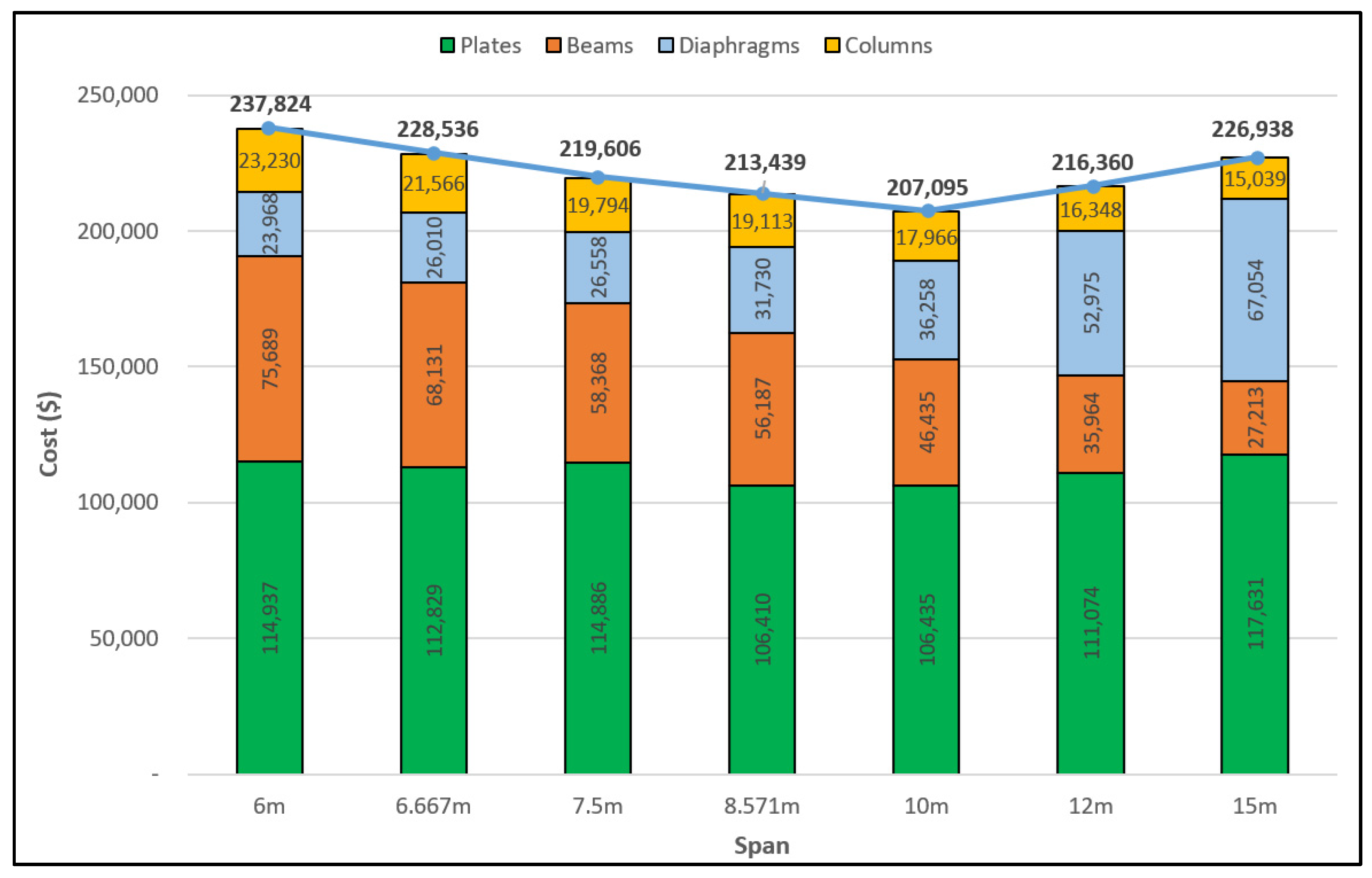
After finding that the DE algorithm performed the best among the three metaheuristic algorithms, it is used to find the optimum design of the three-segment folded plate roof type under different transverse span settings. As done in with the V-type folded plate roof, the overall building length is divided into equal transverse spans of 6 m, 6.667 m, 7.5 m, 8.571 m, 10 m, 12 m, and 15 m for buildings with nine through three internal supports, respectively. The number of grouped design variables then becomes 12 for the three-segment type folded plate roof building. The internal controlling parameter values of the DE algorithm are presented in Table 13. The amounts representing the cost of each element for the optimum solution at each transverse span are represented in Figure 24.
As shown in Figure 24, the transverse span that generates the optimum solution for the three-segment type folded plate roofs is 10 m (a building having five internal supports). The optimum solution is close to the best solution found by the DE algorithm in its 10 trial runs, as discussed in Section 4.2. Unlike the V-type folded plate roofs, the cost of plates remained approximately the same for the entirety of the transverse spans studied. This shows that this type of folded plate is suitable even for 15 m long transverse spans. Like the V-type folded plates, the cost of beams and diaphragms are inversely related; for shorter transverse spans, the cost of beams dominates and takes more than three times the cost of diaphragms representing a large portion of the entire cost, while in longer spans the opposite is true. Finally, the cost of the supporting columns in this type of roof is also relatively fixed for all the spans, and it represents a small portion of the entire cost.
5. Conclusions
It is shown that the optimum design of reinforced concrete V- and three-segment types of folded plate structures with their auxiliary and supporting members in accordance with ACI 318-11 can be achieved using different metaheuristic algorithms. The design problems consider the strength, serviceability, and applicability requirements set by the code. Additionally, all the detailing provisions, such as development and hook lengths of both longitudinal and transverse reinforcements, are considered while estimating the overall cost of reinforcement. In both roof types, the DE algorithm achieved the best optimization results proving its suitability for the optimization of such structures. Studying the effects of changing the transverse span while maintaining the overall dimensions of the building gave an indication of how the optimum cost varies with the percentages represented by each member. For the V-type folded plate roofs, the best optimum transverse span is 8.571 m. While for the three-segment type folded plate roofs, the best optimum transverse span is 10 m. These spans indicate that it is preferable to have transverse to longitudinal span ratios of 1:3 and 1:2.5 for V- and three-segment types of folded plate roofs, respectively. The cost that each member represents of the overall cost of building differs depending on the span being considered; for shorter transverse spans, it is mainly consumed by the plates and beams, while for the longer transverse spans, it is consumed by the plates and diaphragms. The cost of supporting columns remains almost the same for all transverse spans. It is found that the cost of formwork constitutes almost two-thirds of the overall material cost of the building, while the concrete and reinforcements together represent only one-third. This makes folded plate structures, compared to other types of structures, economical and environment-friendly construction. It should be noticed that the formwork can be removed and reused once the members develop their required strengths. This indicates the profitability of folded plate structures. Furthermore, it also implies less emission to the atmosphere due to the production of less amount of construction materials.
Author Contributions
Conceptualization, S.Y. and M.P.S.; methodology, S.Y.; software, S.Y.; validation, M.P.S.; writing—original draft preparation, S.Y.; writing—review and editing, S.Y., M.P.S., S.K. and Z.W.G.; supervision, M.P.S. and Z.W.G.; funding acquisition, Z.W.G. All authors have read and agreed to the published version of the manuscript.
Funding
This research was supported by the Energy Cloud R&D Program through the National Research Foundation of Korea (NRF) funded by the Ministry of Science, ICT (2019M3F2A1073164).
Institutional Review Board Statement
Not applicable.
Informed Consent Statement
Not applicable.
Data Availability Statement
Not applicable.
Conflicts of Interest
The authors declare no conflict of interest.
References
- Bar-Yoseph, P.; Hersckovitz, I. Analysis of folded plate structures. Thin-Walled Struct. 1989, 7, 139–158. [Google Scholar] [CrossRef]
- Wilby, C.B. Concrete Folded Plate Roofs; Elsevier-Butterworth-Heinemann: Oxford, UK, 2005; ISBN 0-340-66266-2. [Google Scholar]
- Varghese, P.C. Design of Reinforced Concrete Shells and Folded Plates; PHI Learning Private Ltd.: New Delhi, India, 2010; ISBN 978-81-203-4111-1. [Google Scholar]
- Gomez, R.A. Design of Folded Plates, PDH Online Course S275 (5PDH), PDH Center. 2013. Available online: https://pdhonline.com/courses/s275/s275content.pdf (accessed on 14 April 2022).
- Sarma, K.C.; Adeli, H. Cost optimization of concrete structures. J. Struct. Eng. 1998, 124, 570–578. [Google Scholar] [CrossRef]
- Kostem, C.N. Optimization of folded plate roofs. Comput. Struct. 1973, 3, 125–132. [Google Scholar] [CrossRef]
- ACI 318-11; Building Code Requirements for Structural Concrete and Commentary. American Concrete Institute Committee: Farmington Hills, MI, USA, 2011; ISBN 978-0-87031-744-6.
- ACI.318.2-14; Building Code Requirements for Concrete Thin Shells and Commentary. American Concrete Institute Committee: Farmington Hills, MI, USA, 2014; ISBN 978-0-87031-934-1.
- Mathworks. Available online: https://www.mathworks.com/products/matlab.html (accessed on 25 April 2021).
- Computers & Structures, Inc. Available online: https://www.csiamerica.com/products/sap2000 (accessed on 25 April 2021).
- ASCE/SEI 7-05; Minimum Design Loads for Buildings and Other Structures. American Society of Civil Engineers: Farmington Hills, MI, USA, 2005; ISBN 0-7844-0831-9.
- Kaveh, A. Advances in Metaheuristic Algorithms for Optimal Design of Structures; Springer: Berlin/Heidelberg, Germany, 2017. [Google Scholar] [CrossRef]
- Latif, M.A.; Saka, M.P. Optimum design of tied-arch bridges under code requirements using enhanced artificial bee colony algorithm. Adv. Eng. Softw. 2019, 135, 102685. [Google Scholar] [CrossRef]
- Yousif, S.; Saka, M.P. Optimum design of post-tensioned flat slabs with its columns to ACI 318-11 using population-based beetle antenna search algorithm. Comput. Struct. Int. J. 2021, 256, 106520. [Google Scholar] [CrossRef]
- Wang, Z.; Tang, H.; Li, P. Optimum design of truss structures based on differential evolution strategy. In Proceedings of the International Conference on Information Engineering and Computer Science, Wuhan, China, 1–5 December 2009. [Google Scholar] [CrossRef]
- Saka, M.P.; Geem, Z.W. Mathematical and metaheuristic applications in design optimization of steel frame structures: An extensive review. Math. Probl. Eng. 2012, 2013, 271031. [Google Scholar] [CrossRef] [Green Version]
- Saka, M.P. Design code optimization of steel structures using adaptive harmony search algorithm. In Harmony Search Algorithms for Structural Design Optimization; Series: Studies in Computational Intelligence; Geem, Z.W., Ed.; Springer: Berlin/Heidelberg, Germany, 2009; Volume 239. [Google Scholar] [CrossRef]
- Saka, M.P.; Dogan, E.; Aydogdu, I. Review and analysis of swarm-intelligence based algorithms. In Swarm Intelligence and Bio-Inspired Computation; Yang, X.S., Cui, Z., Xiao, R., Gandomi, A.H., Karamanoglu, M., Eds.; Elsevier: Amsterdam, The Netherlands, 2013; pp. 25–47. [Google Scholar] [CrossRef]
- Kaveh, A.; Ghazaan, M.A.I. Metaheuristic Algorithms for Optimal Design of Real-Size Structures; Springer: Berlin/Heidelberg, Germany, 2018. [Google Scholar] [CrossRef]
- Kaveh, A.; Eslamlu, A.D. Metaheuristic Optimization Algorithms in Civil Engineering: New Applications; Springer: Berlin/Heidelberg, Germany, 2017. [Google Scholar] [CrossRef]
- Jiang, X.; Li, S. BAS: Beetle Antennae Search Algorithm for Optimization Problems. Int. J. Robot. Control. 2018, 1, 1. [Google Scholar] [CrossRef]
- Yousif, S.; Saka, M.P. Enhanced beetle antenna search: A swarm intelligence algorithm. Asian J. Civ. Eng. 2021, 22, 73–91. [Google Scholar] [CrossRef]
- Karaboga, D. An Idea Based on Honeybee Swarm for Numerical Optimization Technical Report-TR06; Computer Engineering Department, Engineering Faculty, Erciyes University: Kayseri, Turkey, 2005. [Google Scholar]
- Karaboga, D.; Basturk, B. A powerful and efficient algorithm for numerical function optimization: Artificial bee colony (ABC) algorithm. J. Glob. Optim. 2007, 39, 459–471. [Google Scholar] [CrossRef]
- Karaboga, D.; Basturk, B. On the performance of artificial bee colony (ABC) algorithm. Appl. Soft Comput. 2008, 8, 687–697. [Google Scholar] [CrossRef]
- Karaboga, D.; Akay, B. A modified artificial bee colony (ABC) algorithm for constrained optimization problems. Appl. Soft Comput. 2011, 11, 3021–3031. [Google Scholar] [CrossRef]
- Storn, R.; Price, K. Differential evolution- A simple and efficient heuristic for global optimization over continuous spaces. J. Glob. Optim. 1997, 11, 341–359. [Google Scholar] [CrossRef]
Figure 1.
Typical folded plate building roof plan.
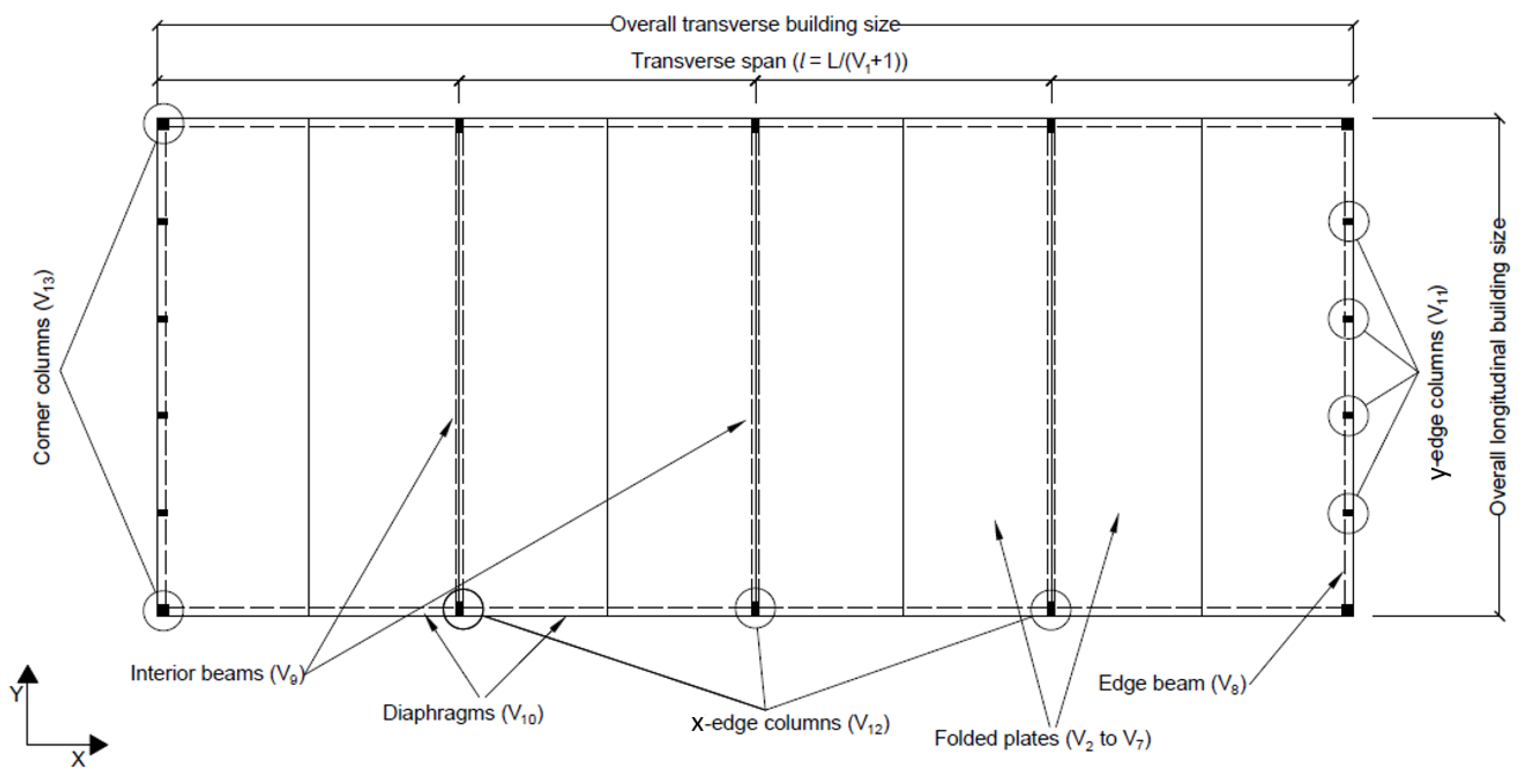
Figure 2.
Folded plate roof number of internal supports design variable (V1): (A) “V” type folded plate roofed building elevation view; (B) Three-segment type folded plate roofed building elevation view.
Figure 2.
Folded plate roof number of internal supports design variable (V1): (A) “V” type folded plate roofed building elevation view; (B) Three-segment type folded plate roofed building elevation view.
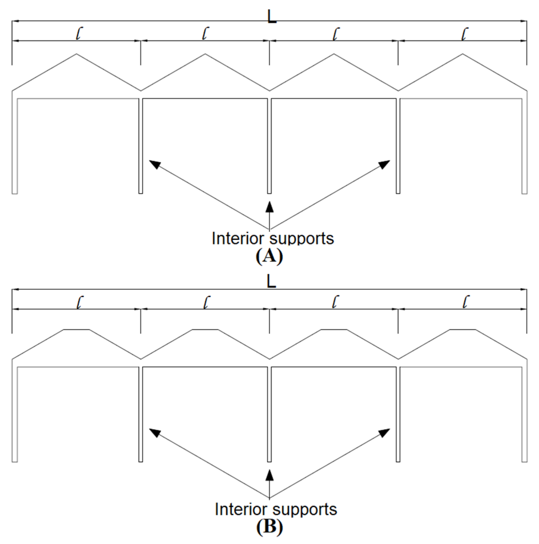
Figure 3.
Folded plate roof section controlling design variables (V2 through V7): (A) “V” type folded plate roof section view; (B) Three-segment type folded plate roof section view.
Figure 3.
Folded plate roof section controlling design variables (V2 through V7): (A) “V” type folded plate roof section view; (B) Three-segment type folded plate roof section view.
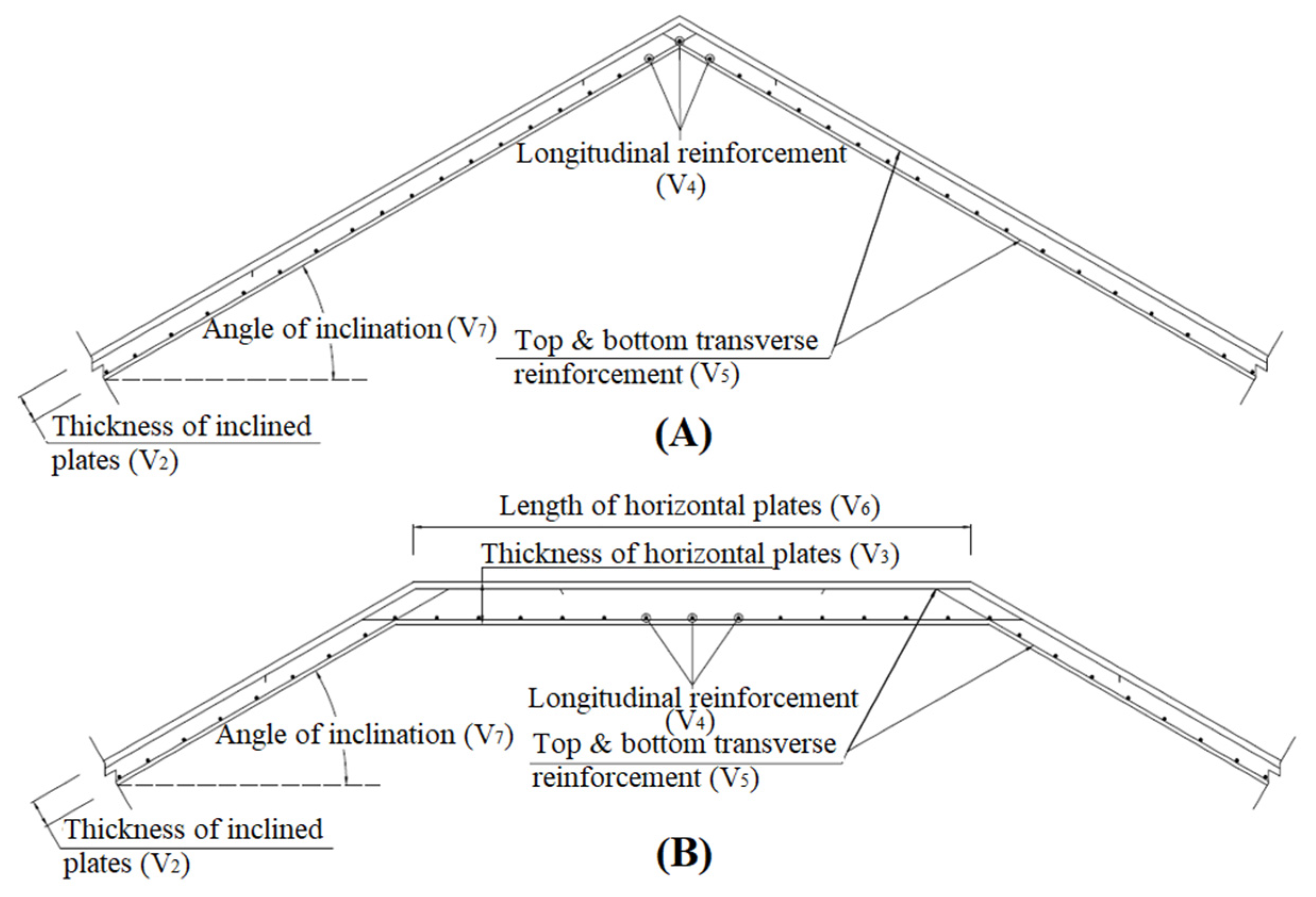
Figure 4.
Beams controlling design variables (V8 and V9): (A) Beam section view; (B) Beam elevation view.
Figure 4.
Beams controlling design variables (V8 and V9): (A) Beam section view; (B) Beam elevation view.
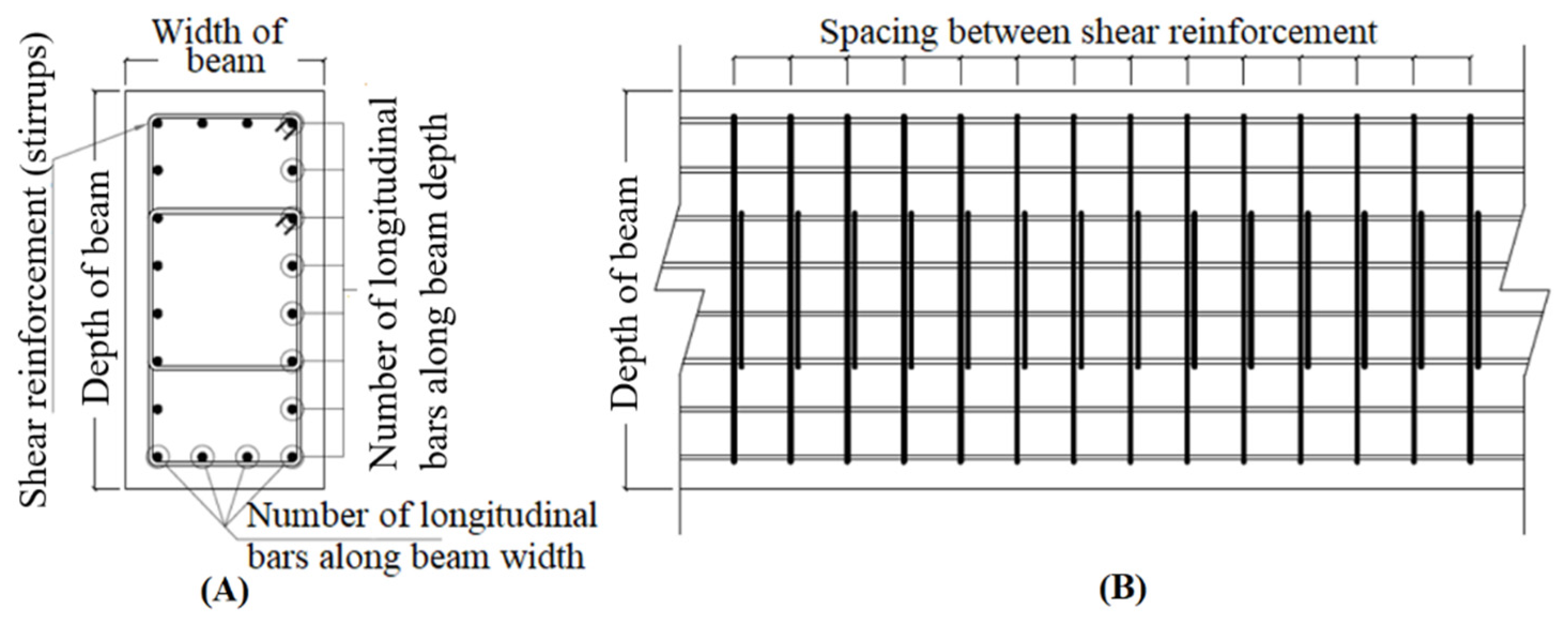
Figure 5.
Diaphragms controlling design variables (V10): (A) Elevation view of diaphragms in “V” type folded plates roofed building; (B) Elevation view of diaphragms in three-segment type folded plates roofed buildings; (C) Section A-A view; (D) Section B-B view.
Figure 5.
Diaphragms controlling design variables (V10): (A) Elevation view of diaphragms in “V” type folded plates roofed building; (B) Elevation view of diaphragms in three-segment type folded plates roofed buildings; (C) Section A-A view; (D) Section B-B view.
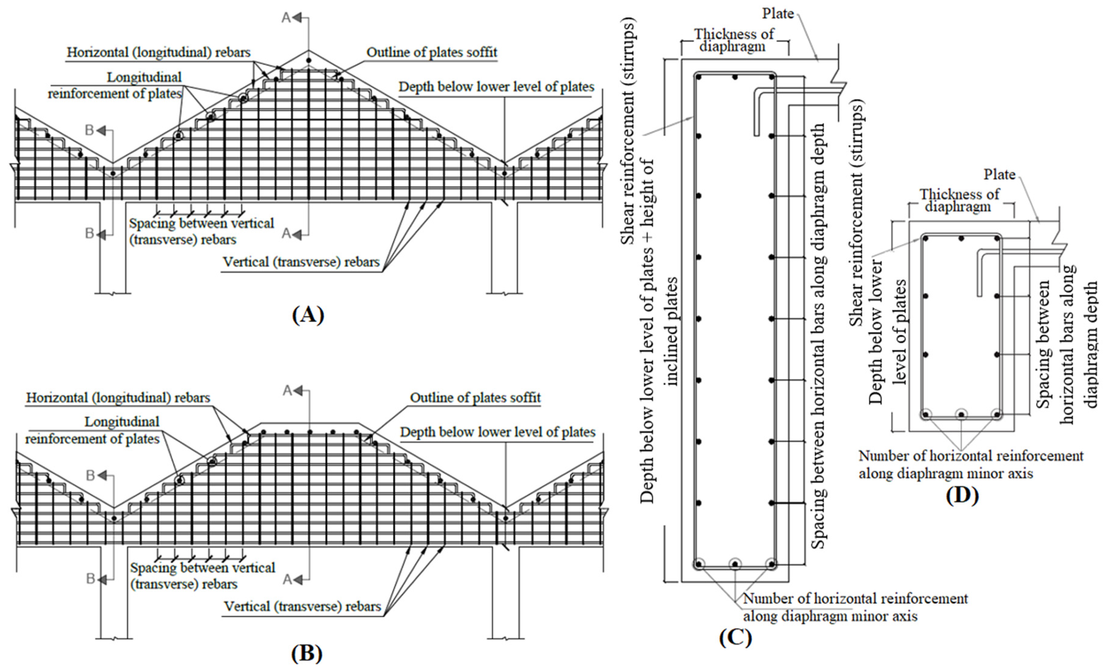
Figure 6.
Columns controlling design variables (V11, V12, and V13): (A) Columns section view; (B) Columns elevation view.
Figure 6.
Columns controlling design variables (V11, V12, and V13): (A) Columns section view; (B) Columns elevation view.
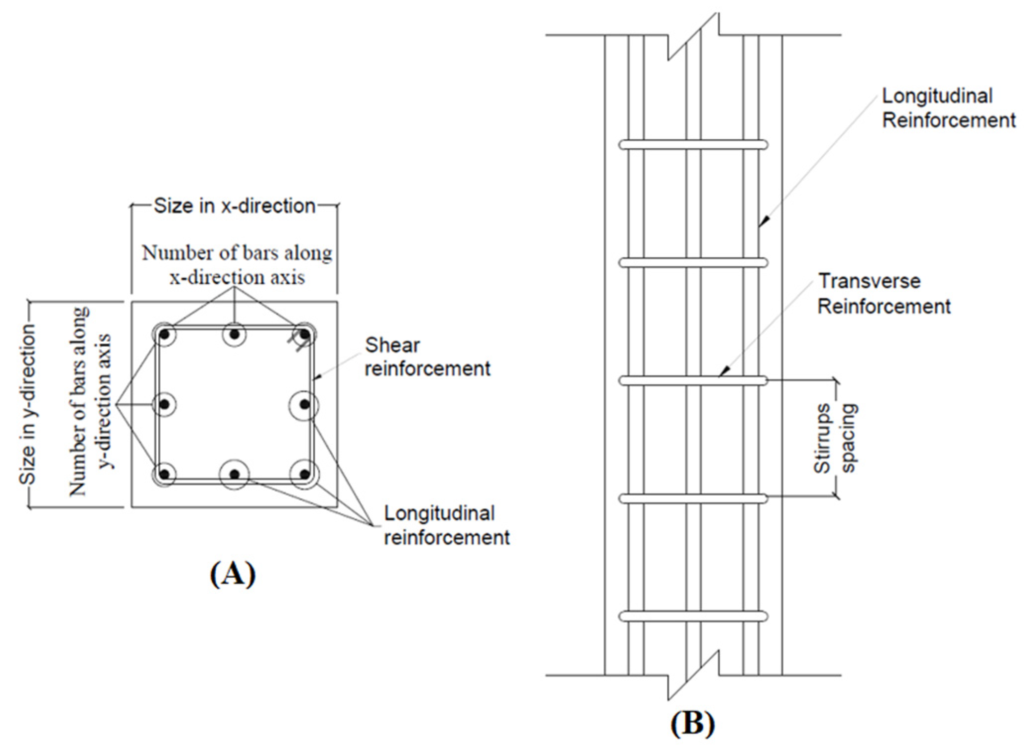
Figure 7.
Interaction diagram linear approximation.
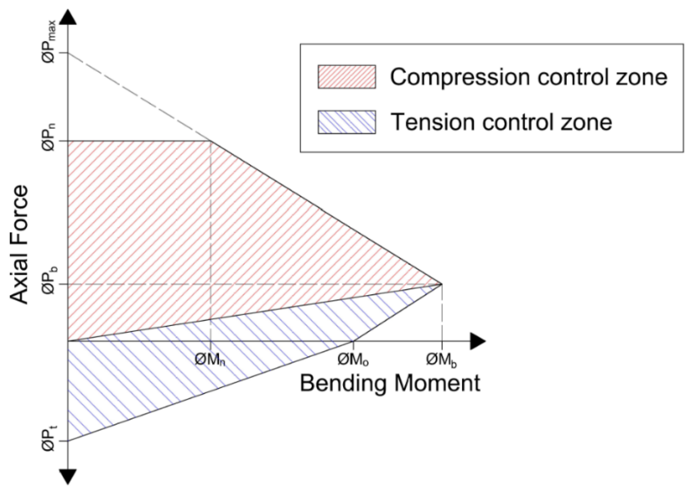
Figure 8.
Flow chart of pbBAS algorithm.
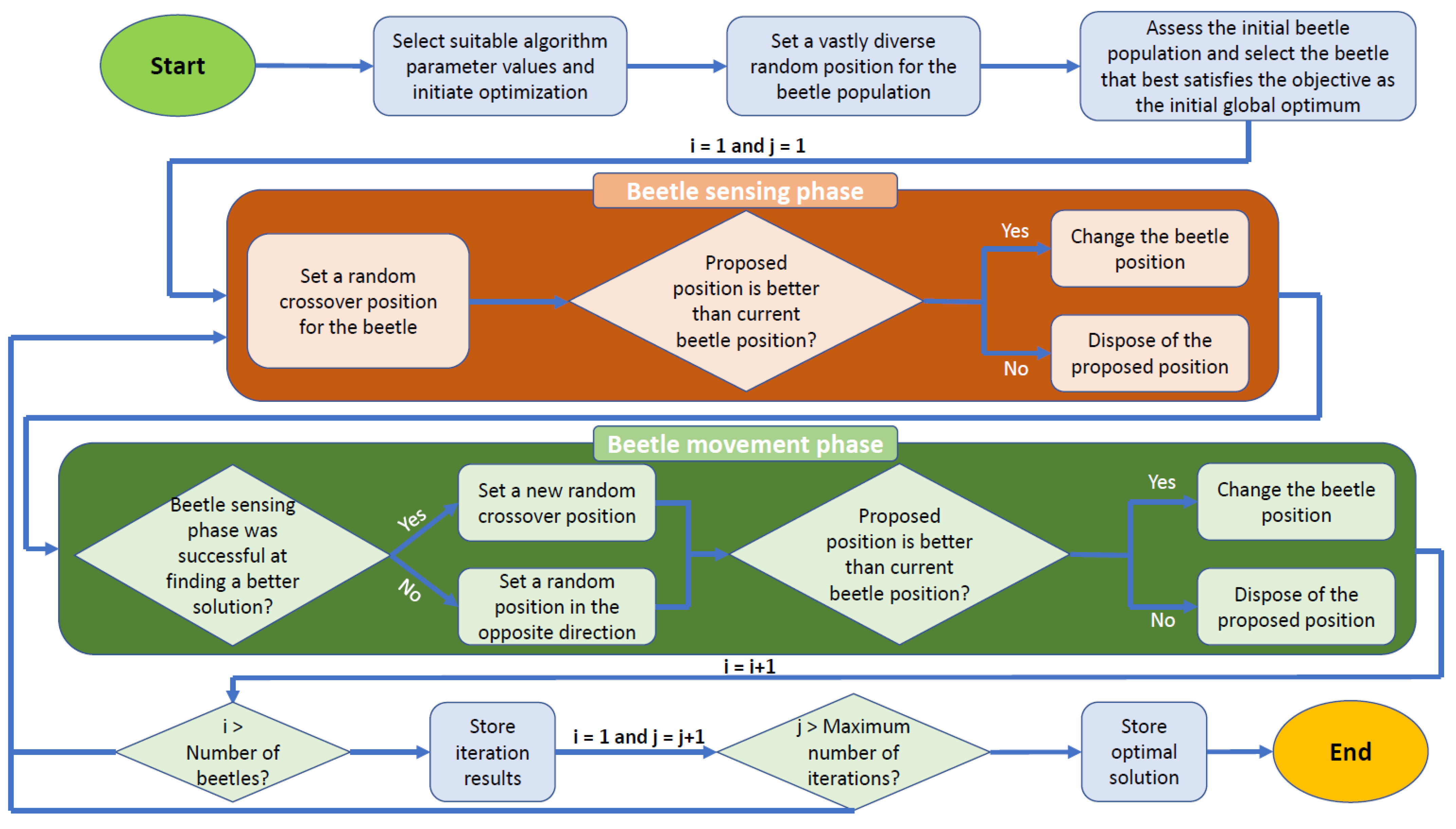
Figure 9.
Flow chart for general metaheuristic algorithm in MATLAB.
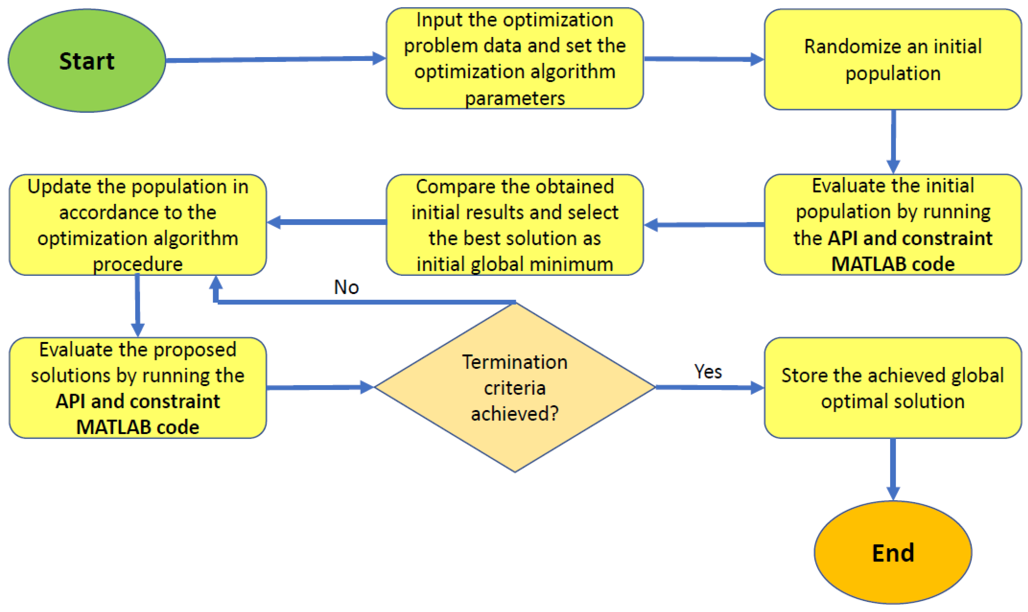
Figure 10.
Flow chart for API and constraints in MATLAB.
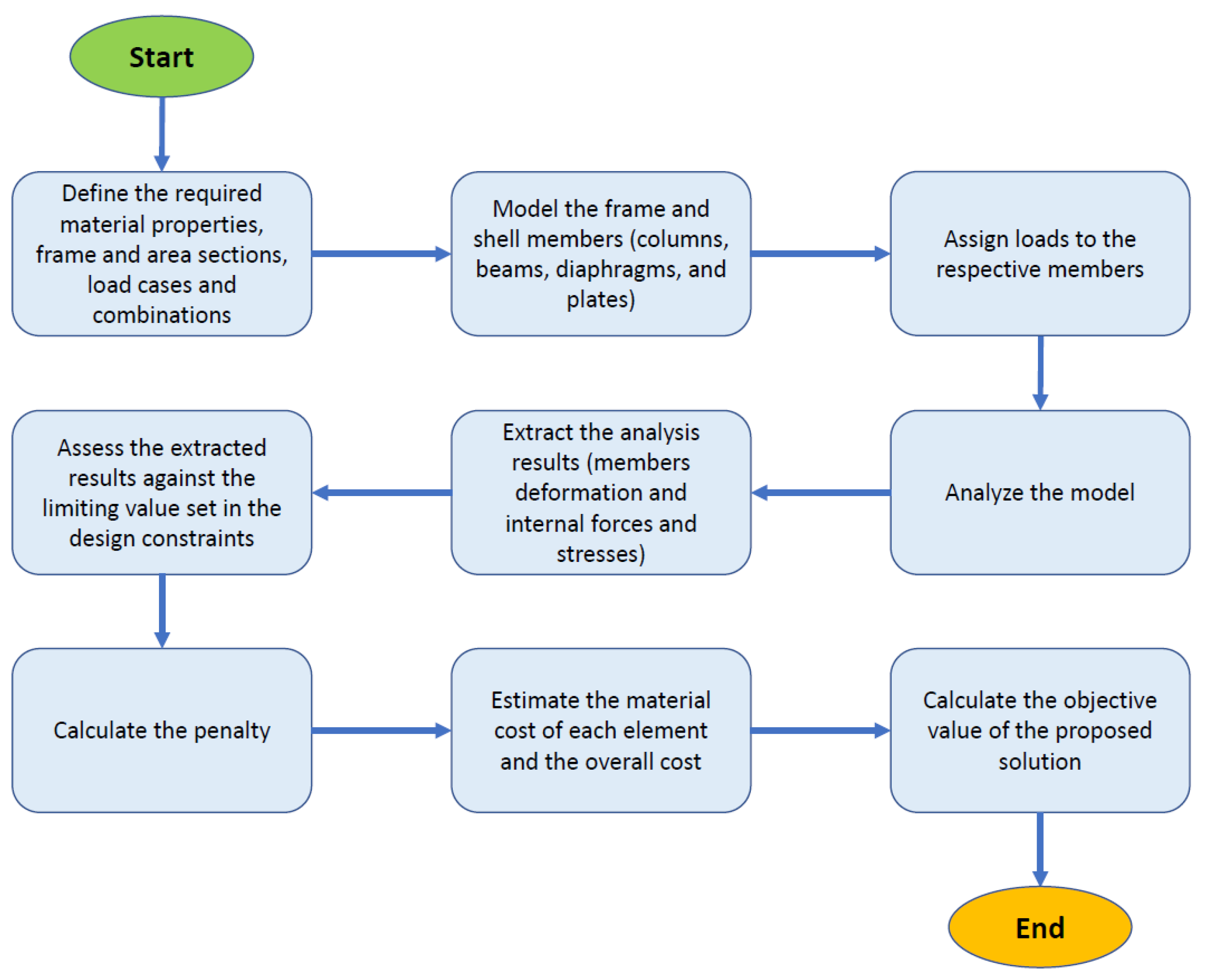
Figure 11.
V-type folded plate roof problem: (A) 3D view; (B) Plan view; (C) South elevation view; (D) East elevation view.
Figure 11.
V-type folded plate roof problem: (A) 3D view; (B) Plan view; (C) South elevation view; (D) East elevation view.
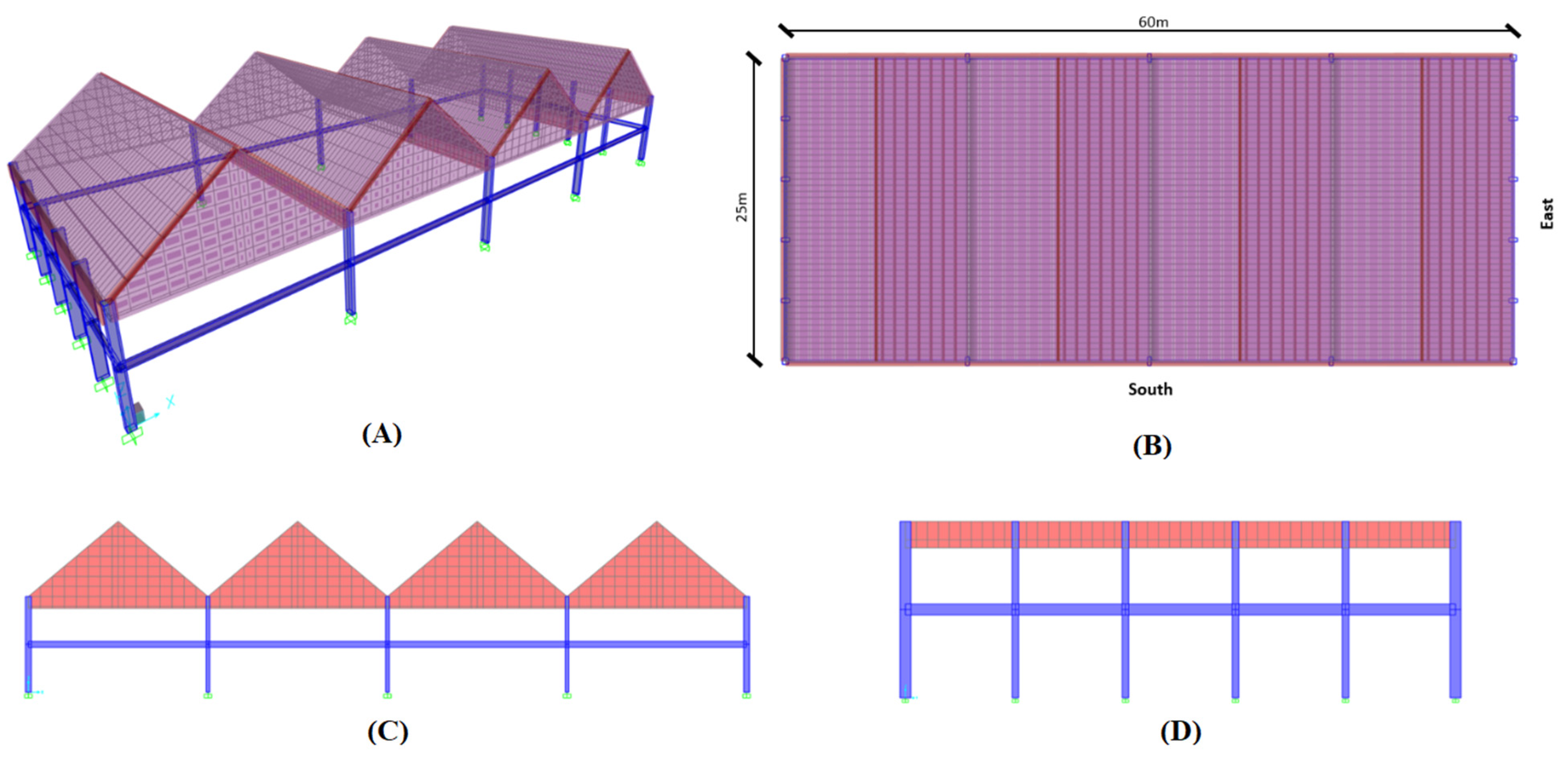
Figure 12.
Design history of the best run achieved by each metaheuristic algorithm for the V-type folded plate roof problem.
Figure 12.
Design history of the best run achieved by each metaheuristic algorithm for the V-type folded plate roof problem.
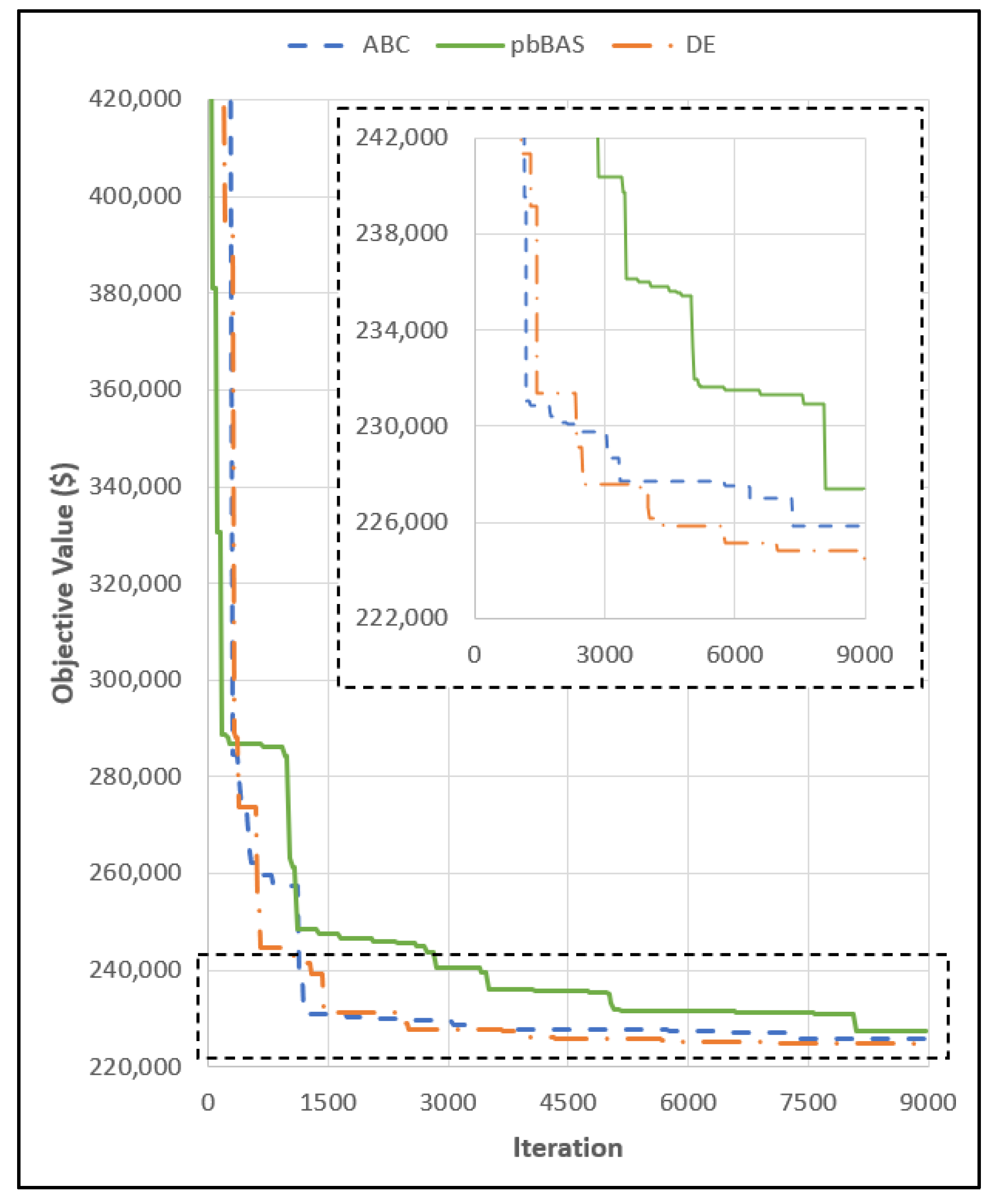
Figure 13.
Design history of the sample average of the 10 runs achieved by each metaheuristic algorithm for the V-type folded plate roof problem.
Figure 13.
Design history of the sample average of the 10 runs achieved by each metaheuristic algorithm for the V-type folded plate roof problem.
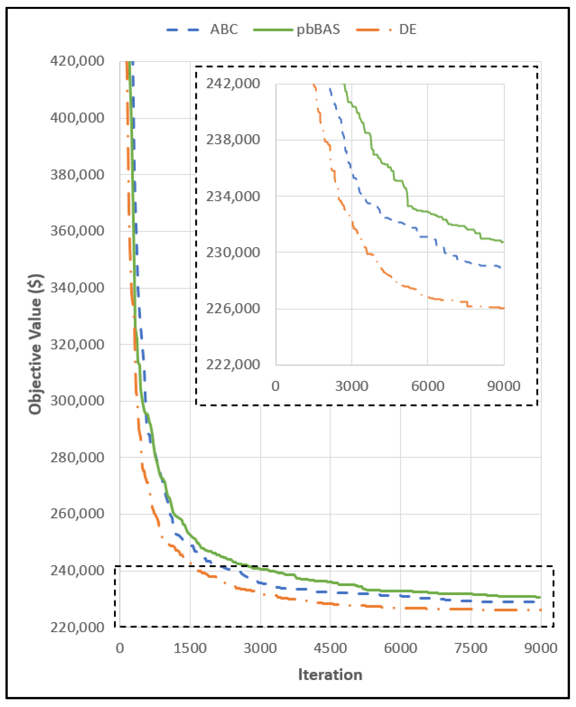
Figure 14.
Design history of the worst run achieved by each metaheuristic algorithm for the V-type folded plate roof problem.
Figure 14.
Design history of the worst run achieved by each metaheuristic algorithm for the V-type folded plate roof problem.
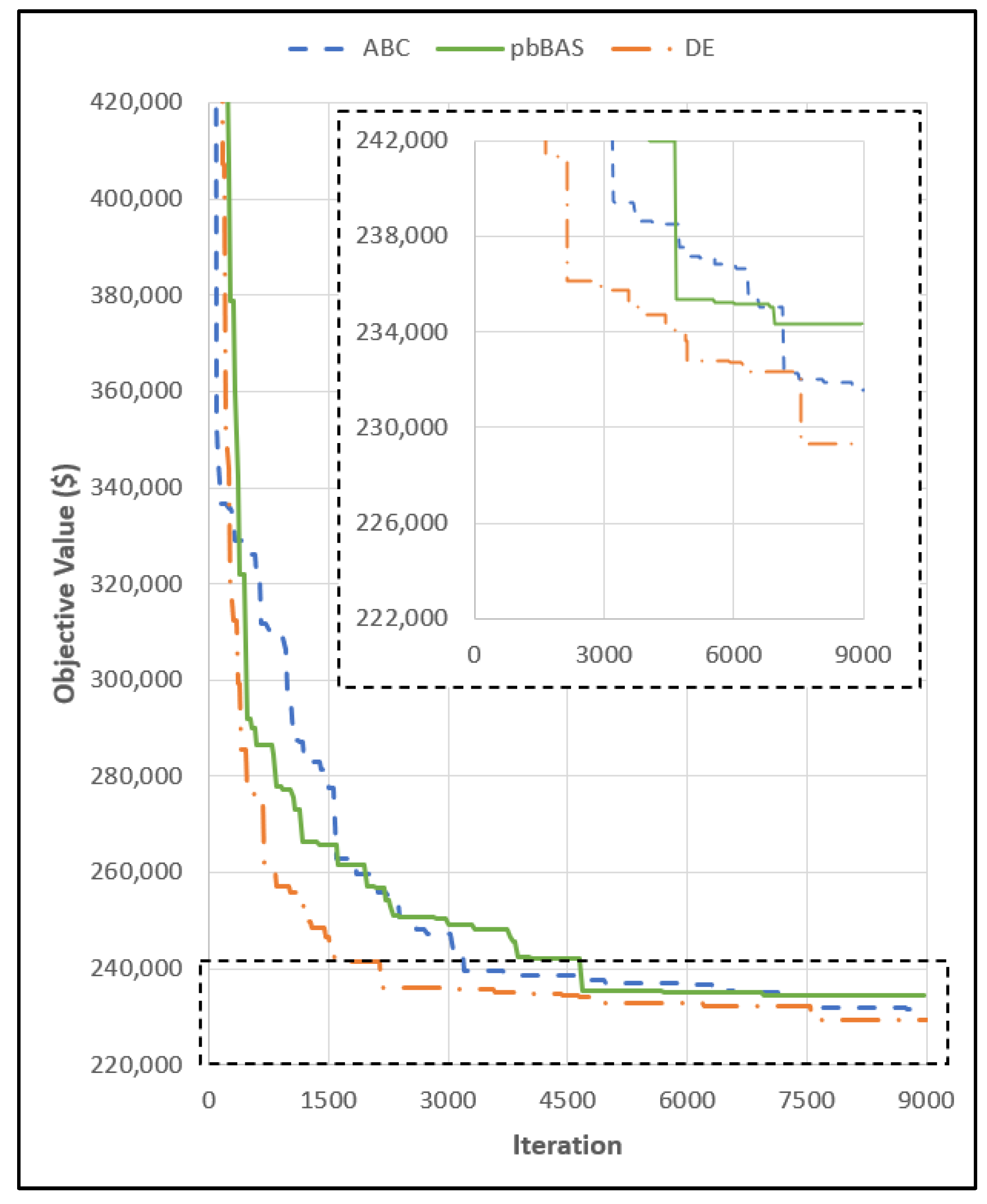
Figure 15.
Box plot of the results achieved by each metaheuristic algorithm after 10 runs for the V-type folded plate roof problem.
Figure 15.
Box plot of the results achieved by each metaheuristic algorithm after 10 runs for the V-type folded plate roof problem.
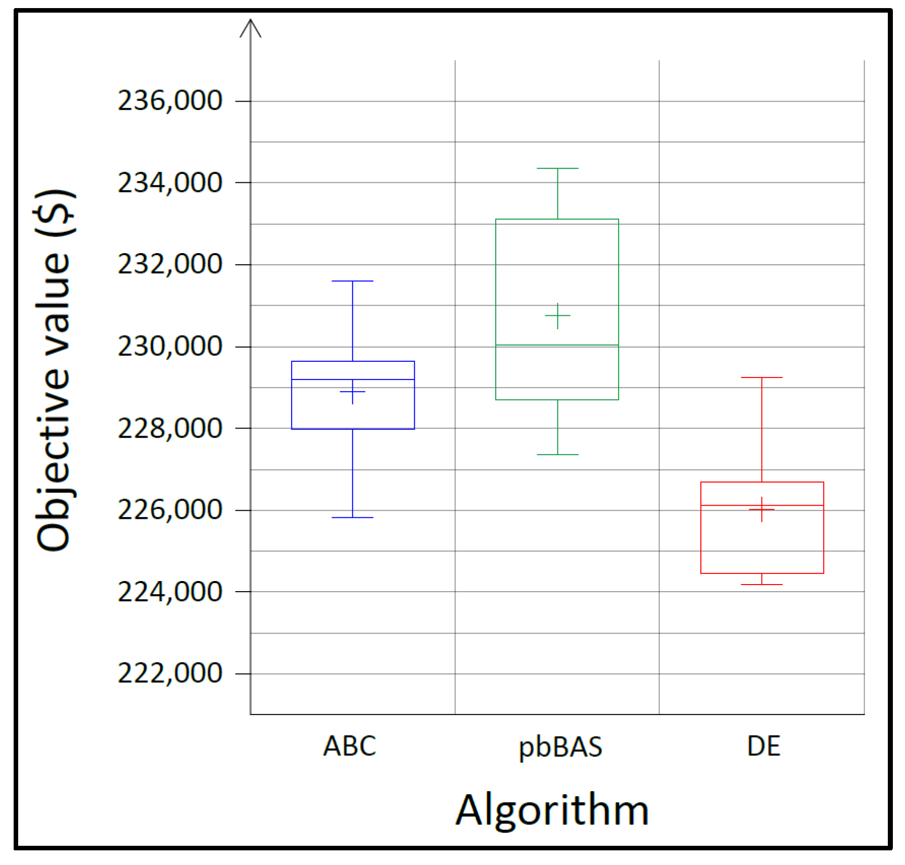
Figure 16.
Pie chart of the cost components for the optimum design achieved in the V-type folded plate roof problem.
Figure 16.
Pie chart of the cost components for the optimum design achieved in the V-type folded plate roof problem.

Figure 17.
Three-segment type folded plate roof problem: (A) 3D view; (B) Plan view; (C) South elevation view; (D) East elevation view.
Figure 17.
Three-segment type folded plate roof problem: (A) 3D view; (B) Plan view; (C) South elevation view; (D) East elevation view.
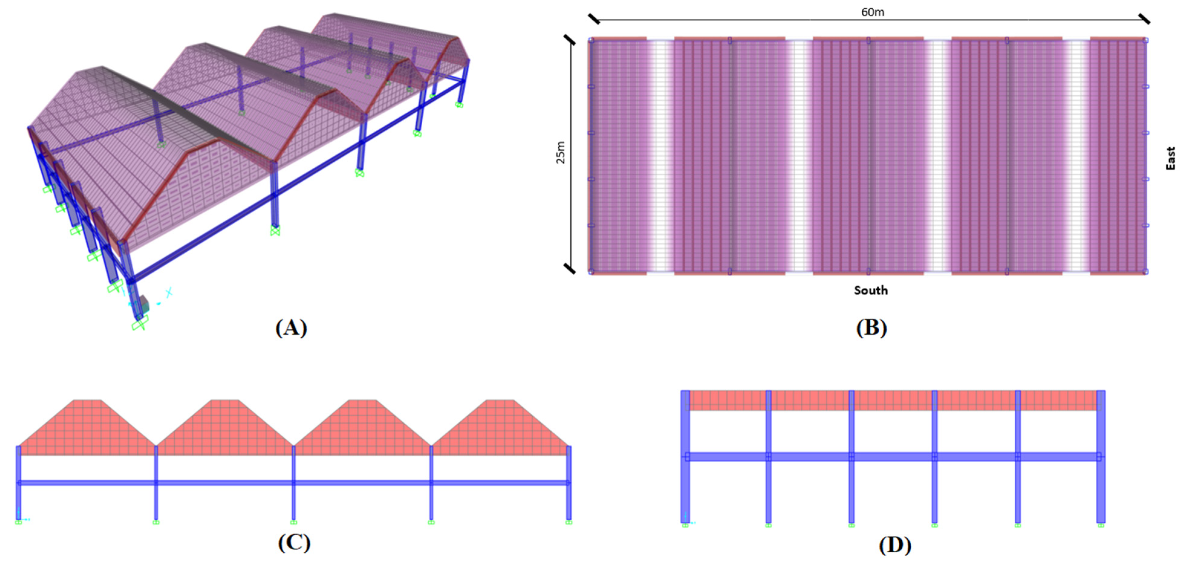
Figure 18.
Design history of the best run achieved by each metaheuristic algorithm for the three-segment type folded plate roof problem.
Figure 18.
Design history of the best run achieved by each metaheuristic algorithm for the three-segment type folded plate roof problem.
Figure 19.
Design history of the sample average of the 10 runs achieved by each metaheuristic algorithm for the three-segment type folded plate roof problem.
Figure 19.
Design history of the sample average of the 10 runs achieved by each metaheuristic algorithm for the three-segment type folded plate roof problem.

Figure 20.
Design history of the worst run achieved by each metaheuristic algorithm for the three-segment type folded plate roof problem.
Figure 20.
Design history of the worst run achieved by each metaheuristic algorithm for the three-segment type folded plate roof problem.
Figure 21.
Box plot of the results achieved by each metaheuristic algorithm after 10 runs for the three-segment type folded plate roof problem.
Figure 21.
Box plot of the results achieved by each metaheuristic algorithm after 10 runs for the three-segment type folded plate roof problem.
Figure 22.
Pie chart of the cost components for the optimum design achieved in the three-segment type folded plate roof problem.
Figure 22.
Pie chart of the cost components for the optimum design achieved in the three-segment type folded plate roof problem.
Figure 23.
Cost components of the optimum designs achieved at different transverse spans for the V-type folded plate roof building.
Figure 23.
Cost components of the optimum designs achieved at different transverse spans for the V-type folded plate roof building.
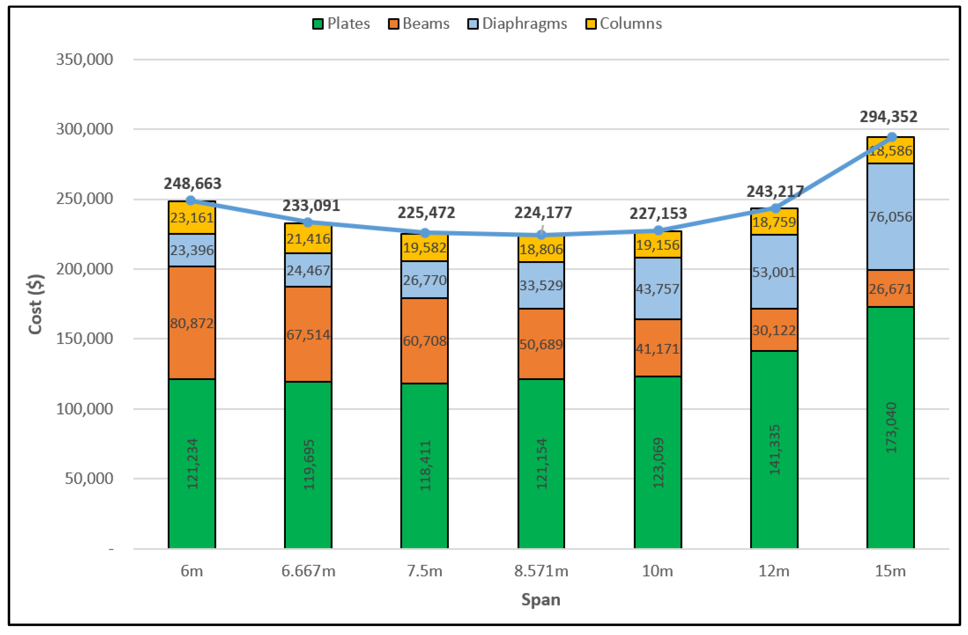
Figure 24.
Cost components of the optimum designs achieved at different transverse spans for the three-segment type folded plate roof building.
Figure 24.
Cost components of the optimum designs achieved at different transverse spans for the three-segment type folded plate roof building.

Table 1.
Design variable classes.
| Design Variables | Description | List of Details Grouped in the Design Variable | Number of Variables in Problem | |
|---|---|---|---|---|
| 1 | 2 | |||
| V1 | Number of internal intermediate supports | No grouping | 1 | 1 |
| V2 & V3 | Plate thickness I | No grouping | 1 | 2 |
| V4 & V5 | Plate’s reinforcement configuration in each direction II | Two grouped details:
| 2 | 2 |
| V6 | Length of horizontal plate III | No grouping | 0 | 1 |
| V7 | Angle of plate’s inclination IV | No grouping | 1 | 1 |
| V8 & V9 | Beams sectional details V | Seven grouped details:
| 2 | 2 |
| V10 | Diaphragm sectional details VI | Seven grouped details:
| 1 | 1 |
| V11–V13 | Columns sectional details VII | Seven grouped details:
| 3 | 3 |
| Total | 11 | 13 | ||
I: two different plate thicknesses are allowed in the model for problem (2): the first is for the inclined plate, and the second is for the horizontal plate. II: two configurations of plate reinforcement: the first is for the longitudinal reinforcement, and the second is for the transverse reinforcement. III: for problem (2), one length is set for all the horizontal plates at each span. IV: one angle of inclination is set for all the inclined plates; the angle is measured in degrees from the horizontal axis. V: two different beam sections are modeled: edge beams and internal beams. VI: one diaphragm section is set on both sides of the building. VII: three different column sections are modeled: x-edge columns, y-edge columns, and corner columns.
Table 2.
Design pools of folded plate variables.
| Details | Pool | ||
|---|---|---|---|
| Number of interior supports (Nos.) | 3:1:9 | ||
| Thickness (mm) | 70:10:200 | ||
| Longitudinal and Transverse reinforcement | Diameter (mm) | {8, 10, 12, 16, 20} | |
| Spacing (mm) | For 8 mm diameter | {200, 250, 300} | |
| For 10 mm diameter | {200, 250} | ||
| For 12 mm diameter | {150, 200, 250} | ||
| For 16 mm diameter | {150, 200} | ||
| For 20 mm diameter | {100, 150, 200} | ||
| Angle of plates inclination (for inclined plates measured from the horizontal axis in degrees) | 5:1:40 | ||
| Length of horizontal plates (mm) | 500:500:5000 | ||
Table 3.
Design pools of edge and internal beam variables.
| Details | Pool | |||
|---|---|---|---|---|
| Size | Depth (mm) | 500:100:1200 | ||
| Width (mm) | For depth of 500 mm | {200} | ||
| For depth of 600 mm | {200, 250} | |||
| For depth of 700 mm | {250, 300} | |||
| For depth of 800 mm | {300, 350} | |||
| For depth of 900 mm | {350} | |||
| For depth of 1000 mm | {350, 400} | |||
| For depth of 1100 mm and 1200 mm | {400} | |||
| Longitudinal reinforcement | Diameter (mm) | For 200 × 500 beams | {12, 16} | |
| For 200 × 600 beams | {16, 20} | |||
| For 250 × 600 beams | {20} | |||
| For 250 × 700 beams | {16, 20} | |||
| For 300 × 700 beams | {20} | |||
| For 300 × 800 or larger beams | {20, 25} | |||
| Number of bars along (Nos.) | Minor axis | For 200 mm wide | {2} | |
| For 250 mm and 300 mm width | {3} | |||
| For 350 mm and 400 mm width | {4} | |||
| Major axis | For 500 mm depth | {5, 6} | ||
| For 600 mm depth | {5, 6, 7} | |||
| For 700 mm depth | {6, 7, 8} | |||
| For 800 mm depth | {7, 8, 9} | |||
| For 900 mm depth | {8, 9, 10} | |||
| For 1000 mm depth | {9, 10, 11} | |||
| For 1100 mm and 1200 mm depth | {10, 11, 12} | |||
| Shear reinforcement | Diameter (mm) | {8, 10, 12} | ||
| Spacing (mm) | For 8 mm diameter | {250, 300} | ||
| For 10 mm diameter | {200, 250} | |||
| For 12 mm diameter | {100, 150, 200} | |||
Table 4.
Diaphragm variables design pools.
| Details | Pool | ||
|---|---|---|---|
| Size | Depth below inclined plates bottom level (mm) | 500:100:1000 | |
| Thickness (mm) | For depth of 500 mm | {200, 250} | |
| For depth of 600 mm | {250, 300} | ||
| For depth of 700 mm | {300, 350} | ||
| For depth of 800 mm | {350} | ||
| For depth of 900 mm | {350, 400} | ||
| For depth of 1000 mm | {400} | ||
| Horizontal (longitudinal) reinforcement | Diameter (mm) | For 200 mm thickness | {12, 16} |
| For 250 mm and 300 mm thickness | {16, 20} | ||
| For 350 mm thickness | {20, 25} | ||
| For 400 mm thickness | {25} | ||
| Number of bars along minor axis (Nos.) | For 200 mm thickness | {2} | |
| For 250 mm thickness | {2, 3} | ||
| For 300 mm thickness | {3} | ||
| For 350 mm thickness | {4} | ||
| For 400 mm thickness | {5} | ||
| Spacing along Major axis (mm) | {100, 150, 200} | ||
| Vertical (transverse) reinforcement | Diameter (mm) | {10, 12, 16} | |
| Spacing (mm) | For 10 mm diameter | {250, 300} | |
| For 12 mm diameter | {200, 250} | ||
| For 16 mm diameter | {100, 150, 200} | ||
Table 5.
Column variables design pools.
| Details | Pool | |||
|---|---|---|---|---|
| Size | x-edge columns | Along x-direction (mm) | 400:100:700 | |
| Along y-direction (mm) | For 400 mm and 500 mm depths | {200} | ||
| For 600 mm depths | {250, 300} | |||
| For 700 mm depths | {300} | |||
| y-edge columns | Along y-direction (mm) | 400:100:700 | ||
| Along x-direction (mm) | For 400 mm and 500 mm deep | {200} | ||
| For 600 mm depths | {250, 300} | |||
| For 700 mm depths | {300} | |||
| Corner columns | Both directions (mm) | {400, 450, 500} | ||
| Longitudinal reinforcement | Diameter (mm) | x and y-edge columns | For 200 mm widths | {12, 16} |
| For 250 mm widths | {16, 20} | |||
| For 300 mm widths | {20, 25} | |||
| Corner columns | {16, 20} | |||
| x and y-edge columns number of bars along | minor axis (Nos.) | For 200 mm and 250 mm widths | {2} | |
| For 300 mm widths | {3} | |||
| Major axis (Nos.) | For 400 mm depths | {4} | ||
| For 500 mm depths | {5} | |||
| For 600 mm depths | {6} | |||
| For 700 mm depths | {7} | |||
| Corner columns number of bars along both directions (Nos.) | For 400 mm sizes | {4} | ||
| For 450 mm and 500 mm sizes | {4, 5} | |||
| Shear reinforcement | Diameter (mm) | {8, 10, 12} | ||
| Spacing (mm) | For 8 mm diameter | {200, 250, 300} | ||
| For 10 mm diameter | {150, 200, 250} | |||
| For 12 mm diameter | {100, 150, 200} | |||
Table 6.
Expressions used to calculate the objective function, penalty, and costs of each element.
| Element | Equation | Terms Definition |
|---|---|---|
| Penalized Objective function | Ctotal: total cost of materials (actual objective function). Penalty: the value of constraints violation. ε: penalty exponent (taken as 1 for all algorithms) | |
| Penalty | nc: total number of constraints. gi: ith constraint violation value. | |
| Overall cost | Cc: total cost of concrete. Cfw: total cost of formwork. Crs: total cost of reinforcing steel. | |
| Concrete | Uc: unit cost of concrete. Vcp: volume of plates concrete. Vcb: volume of beams concrete. Vcd: volume of diaphragms concrete. Vcc: volume of columns concrete. | |
| Formwork | Ufwh: unit cost of horizontal and vertical formworks. Ufwi: unit cost of inclined formworks. Afwhp: area of horizontal plates formworks. Afwip: area of inclined plates formworks. Afwb: area of beams formworks. Afwd: area of diaphragms formworks. Afwc: area of columns formworks. | |
| Reinforcement | Urs: unit cost of reinforcing steel. Wrsp: total weight of reinforcement used in plates. Wrsb: total weight of reinforcement used in beams. Wrsd: total weight of reinforcement used in diaphragms. Wrsc: total weight of reinforcement used in columns. |
Table 7.
Folded plates’ constraints summary.
| Const. | Description | Constraint Equation | Term’s Definition | Remarks |
|---|---|---|---|---|
| Membrane compression | fc(actual): plates ultimate compressive stress. fc(allowable): compression stress capacity. Ø: compression strength reduction factor (0.65). fcu: ultimate compressive strength of concrete. | |||
| Membrane tension | ft(actual): plates ultimate tensile stress. ft(allowable): tension stress capacity. Ø: tensile strength reduction factor (0.9). fy: reinforcement yield strength. As: area of reinforcement. | |||
| Transverse bending moment | Mu: ultimate transverse bending moment. Mn: nominal bending moment capacity. Ø: bending moment capacity reduction factor (ranges between 0.65 to 0.9). | ACI318-11 Clause 18.7 | ||
| Transverse shear | Vu: ultimate transverse shear force at plates interface. Vc: shear capacity of plate section. Ø: shear strength reduction factor (0.75). | ACI318-11 Clause 11.11 | ||
| Immediate deflection | δi(actual): actual immediate deflection. δi(allowable): immediate deflection limiting value. l: minimum span of plates. | |||
| Long-term deflection | δu(actual): actual long-term deflection. δu(allowable): long-term deflection limiting value. | |||
| Maximum reinforcement spacing | S(Provided): provided reinforcement spacing. S(max): maximum allowed reinforcement spacing. | Otherwise: | ||
| Minimum thickness | h: actual plates thickness. h(min): minimum allowed plate thickness. Øt: diameter of transverse reinforcement. Øl: diameter of longitudinal reinforcement. Cb: bottom face cover (15 mm). Ct: top face cover (25 mm). | |||
| Minimum reinforcement area | As: provided area of reinforcement. As(min): minimum allowable area of reinforcement. b: width of plate strip. | |||
| Maximum reinforcement area | As(max): maximum allowable area of reinforcement. |
Table 8.
Auxiliary members’ constraints summary.
| Const. | Description | Constraint Equation | Terms Definition | Remarks |
|---|---|---|---|---|
| Flexural strength | (1) Axial capacity: (2) Moment capacity: (3) Combined flexural capacity: | Pu: ultimate axial load acting on the section. Mu: ultimate bending moment acting on the section. Pn: axial force capacity of the section under the given ultimate loads. Mn: bending moment capacity of the section under the given ultimate loads. Ø: capacity reduction factor (ranges between 0.65 to 0.9). b: perpendicular section dimension to the bending moment. h: parallel section dimension to the bending moment. | According to the interaction diagram shown in Figure 7. | |
| Shear strength | Vu: ultimate shear force acting on the section. Vc: shear capacity of the section. Ø: shear strength reduction factor (0.75). | ACI318-11 Clause 11.11 | ||
| Minimum reinforcement spacing | S(provided): provided reinforcement spacing. S(min): minimum allowed reinforcement spacing for the section. | = 40 mm | ||
| Maximum reinforcement spacing | S(max): maximum allowed reinforcement spacing for the section. | = 300 mm | ||
| Minimum reinforcement area | As: provided reinforcement area in the section. As(min): minimum allowed reinforcement area for the section. dt: effective depth of furthest layer of reinforcement in tensile face. | |||
| Maximum reinforcement area | As(max): maximum allowed reinforcement area for the section. | |||
| Maximum shear reinforcement spacing | Sv: provided shear reinforcement spacing along the member length. Sv(max): maximum allowed shear reinforcement spacing for the section. Vs: required shear reinforcement capacity to safely allow the section capacity to reach the ultimate shear force. | Otherwise: | ||
| Minimum shear reinforcement area | Av: provided shear reinforcement area per unit length. Av(min): minimum allowed shear reinforcement area for the section. |
Table 9.
Column’s constraints summary.
| Const. | Description | Constraint Equation | Terms Definition | Remarks |
|---|---|---|---|---|
| Flexural strength | (1) Axial capacity: (2) Moment capacity: (3) Combined flexural capacity: | Pu: ultimate axial load acting on the column. Mu: ultimate bending moment acting on the column. Pn: axial force capacity of the column under the given ultimate loads. Mn: bending moment capacity of the column under the given ultimate loads. Ø: capacity reduction factor (ranges between 0.65 to 0.9). b: perpendicular section dimension to the bending moment. h: parallel section dimension to the bending moment. | According to the interaction diagram shown in Figure 7 with the exclusion of the tension part (the part below the x-axis). | |
| Shear strength | Vu: ultimate shear force acting on the column. Vc: shear capacity of the column section. Ø: shear strength reduction factor (0.75). | ACI318-11 Clause 11.11 | ||
| Minimum reinforcement spacing | S(provided): provided reinforcement spacing. S(min): minimum allowed reinforcement spacing for the column section. | = 50 mm | ||
| Maximum reinforcement spacing | S(max): maximum allowed reinforcement spacing for the column section. | = 300 mm | ||
| Minimum reinforcement area | As: provided reinforcement area in the column section. As(min): minimum allowed reinforcement area for the column section. | |||
| Maximum reinforcement area | As(max): maximum allowed reinforcement area for the column section. | |||
| Maximum shear reinforcement spacing | Sv: provided shear reinforcement spacing along the column length. Sv(max): maximum allowed shear reinforcement spacing for the column section. Øl: diameter of longitudinal reinforcement. Øv: diameter of shear reinforcement. | |||
| Minimum shear reinforcement area | Av: provided shear reinforcement area per unit length. Av(min): minimum allowed shear reinforcement area for the column section. |
Table 10.
pbBAS algorithm parameters description.
| Parameters | Description |
|---|---|
| Number of Working Beetles | The working population size of beetles |
| Maximum Number of Evaluations | The maximum number of objective function evaluations |
| P | Probability value for beetle parameter changes (ranges between zero and one) |
Table 11.
Load combinations summary.
| Load Combination | DL | LL | WL | Members Checked against Combination | |
|---|---|---|---|---|---|
| Type | Name | ||||
| Ultimate | 1 | 1.4 | - | - | All members |
| 2 | 1.2 | 0.5 | - | All members | |
| 3 | 1.2 | 1.6 | - | All members | |
| 4~27 | 1.2 | 1.6 | ±0.5 | Columns only | |
| 28~51 | 1.2 | 0.5 | ±1.0 | Columns only | |
| 52~75 | 0.9 | - | ±1.0 | Columns only | |
| Service | Immediate deflection | - | 1.0 | - | Plates only |
| Long-term deflection | 1.835 | 1.20875 | - | Plates only | |
Table 12.
Input data for the V-type folded plate roof building.
| Detail | Value | Unit | |||
|---|---|---|---|---|---|
| Material Properties | Concrete ultimate cylindrical strength | 30 | MPa | ||
| Reinforcement | Yield stress | 420 (Grade 60) | MPa | ||
| Modulus of elasticity | 200 | GPa | |||
| Model | Building overall dimensions | Along x-direction | 25,000 | mm | |
| Along y-direction | 60,000 | mm | |||
| Meshing size | Along x-direction | 1000 | mm | ||
| Along y-direction | 500 | mm | |||
| Number of column lines | Along x-direction | 2 + V1 (variable) | Nos. | ||
| Along y-direction | 6 | Nos. | |||
| Total number of columns | 12 + 2V1 (variable) | Nos. | |||
| Transverse span of plates (l) | mm | ||||
| Longitudinal span of plates | 25,000 | mm | |||
| Building height | To the bottom level of inclined plates | 8000 | mm | ||
| To the top level of inclined plates | mm | ||||
| Load Assignments | Plates superimposed dead load | 1.5 | kPa | ||
| Plates live load (acting on the planer area) | 0.75 | kPa | |||
| Wind load | Basic gust wind speed | 160 | kmh | ||
| Exposure Category | “C” | - | |||
| Importance factor | 1 | - | |||
| Topography factor | 1 | - | |||
| Directional factor | 0.85 | - | |||
| Gust factor | 0.85 | - | |||
| Pressure coefficient | Windward face | +0.8 | - | ||
| Leeward face | −0.5 | - | |||
| Unit Cost * | Concrete | 125 | $/m3 | ||
| Reinforcement | 0.95 | $/kg | |||
| Formwork | Vertical and horizontal | 40 | $/m2 | ||
| Inclined | 50 | $/m2 | |||
*: all unit cost rates are obtained from the material suppliers in Bahrain local market.
Table 13.
Adopted internal parameter values for each metaheuristic algorithm in the V-type folded plate roof building.
Table 13.
Adopted internal parameter values for each metaheuristic algorithm in the V-type folded plate roof building.
| Algorithm | Parameter | Value | |
|---|---|---|---|
| ABC | Number of bees (colony size) | 30 | |
| Number of food sources | 15 | ||
| Maximum number of iterations | 300 | ||
| Trial limit | 300 | ||
| DE | Population size | 20 | |
| Crossover probability | 0.2 | ||
| Maximum number of iterations | 450 | ||
| Scaling factor | Lower bound | 0 | |
| Upper bound | 1 | ||
| pbBAS | Number of beetles | 10 | |
| Probability of beetle movement | 0.1 | ||
| Maximum number of iterations | 450 | ||
Table 14.
Optimum results achieved in the V-type folded plate roof building by each metaheuristic algorithm.
Table 14.
Optimum results achieved in the V-type folded plate roof building by each metaheuristic algorithm.
| Metaheuristic Algorithms | Traditional Design ($) | ||||
|---|---|---|---|---|---|
| ABC ($) | pbBAS ($) | DE ($) | |||
| The optimum results in ascending order | 1 | 225,826.80 | 227,366.24 | 224,177.14 | 283,817.05 |
| 2 | 227,186.97 | 228,635.54 | 224,196.82 | ||
| 3 | 227,980.34 | 228,706.35 | 224,462.70 | ||
| 4 | 228,697.83 | 228,756.96 | 224,556.83 | ||
| 5 | 229,019.23 | 229,861.84 | 225,736.41 | ||
| 6 | 229,376.60 | 230,242.71 | 226,510.54 | ||
| 7 | 229,552.96 | 232,715.97 | 226,538.59 | ||
| 8 | 229,653.36 | 233,123.04 | 226,690.03 | ||
| 9 | 230,138.80 | 233,725.44 | 228,018.30 | ||
| 10 | 231,598.06 | 234,348.75 | 229,249.29 | ||
| Minimum | 225,826.80 | 227,366.24 | 224,177.14 | ||
| Q1 | 227,980.34 | 228,706.35 | 224,462.70 | ||
| Q2 (Median) | 229,197.91 | 230,052.27 | 226,123.48 | ||
| Average | 228,903.09 | 230,748.28 | 226,013.66 | ||
| Q3 | 229,653.36 | 233,123.04 | 226,690.03 | ||
| Maximum | 231,598.06 | 234,348.75 | 229,249.29 | ||
| Standard dev. | 1609.5193 | 2503.6906 | 1723.8909 | ||
Table 15.
The optimum values of folded plates variables obtained by each metaheuristic algorithm for the V-type folded plate roof building.
Table 15.
The optimum values of folded plates variables obtained by each metaheuristic algorithm for the V-type folded plate roof building.
| Design Variable | Detail | Best Optimum Designs | Traditional Design | ||
|---|---|---|---|---|---|
| ABC | pbBAS | DE | |||
| V1 | Number of interior supports | = 8.571 m) | = 8.571 m) | = 8.571 m) | = 12 m) |
| V2 | Thickness of inclined plates | 90 mm | 80 mm | 80 mm | 110 mm |
| V4 | Longitudinal reinforcement configuration | T12@250 mm | T10@200 mm | T10@250 mm | T12@200 mm |
| V5 | Transverse reinforcement configuration | T12@250 mm | T12@200 mm | T12@250 mm | T12@150 mm |
| V7 | Angle of inclination | 30° | 30° | 29° | 40° |
Table 16.
The optimum values of auxiliary members variables obtained by each metaheuristic algorithm for the V-type folded plate roof building.
Table 16.
The optimum values of auxiliary members variables obtained by each metaheuristic algorithm for the V-type folded plate roof building.
| Design Variable | Member | Detail | Best Optimum Designs | Traditional Design | ||
|---|---|---|---|---|---|---|
| ABC | pbBAS | DE | ||||
| V8 | Edge beams | Width | 300 mm | 350 mm | 350 mm | 300 mm |
| Depth | 800 mm | 900 mm | 900 mm | 700 mm | ||
| Diameter of longitudinal reinforcement | 20 mm | 20 mm | 20 mm | 20 mm | ||
| Number of longitudinal rebars along minor axis | 3 Nos. | 4 Nos. | 4 Nos. | 3 Nos. | ||
| Number of longitudinal rebars along major axis | 7 Nos. | 8 Nos. | 8 Nos. | 6 Nos. | ||
| Shear reinforcement configuration | T8@300 mm | T10@250 mm | T8@250 mm | T10@250 mm | ||
| V9 | Interior beams | Width | 350 mm | 350 mm | 400 mm | 400 mm |
| Depth | 1000 mm | 1000 mm | 1100 mm | 1200 mm | ||
| Diameter of longitudinal reinforcement | 25 mm | 25 mm | 25 mm | 20 mm | ||
| Number of longitudinal rebars along minor axis | 4 Nos. | 4 Nos. | 4 Nos. | 4 Nos. | ||
| Number of longitudinal rebars along major axis | 11 Nos. | 11 Nos. | 11 Nos. | 10 Nos. | ||
| Shear reinforcement configuration | T10@200 mm | T10@250 mm | T10@250 mm | T10@250 mm | ||
| V10 | Diaphragms | Thickness | 250 mm | 250 mm | 250 mm | 350 mm |
| Depth of diaphragm below lower level of plates | 500 mm | 500 mm | 500 mm | 800 mm | ||
| Diameter of horizontal reinforcement | 16 mm | 16 mm | 16 mm | 20 mm | ||
| Number of horizontal rebars along minor axis | 3 Nos. | 3 Nos. | 3 Nos. | 4 Nos. | ||
| Spacing between horizontal rebars along major axis | 200 mm | 200 mm | 200 mm | 200 mm | ||
| Vertical reinforcement configuration | T16@200 mm | T16@200 mm | T16@200 mm | T16@150 mm | ||
Table 17.
Optimum values of column’s variables obtained by each metaheuristic algorithm for the V-type folded plate roof building.
Table 17.
Optimum values of column’s variables obtained by each metaheuristic algorithm for the V-type folded plate roof building.
| Design Variable | Member | Detail | Best Optimum Designs | Traditional Design | ||
|---|---|---|---|---|---|---|
| ABC | pbBAS | DE | ||||
| V11 | x-edge columns | Size in x-direction | 400 mm | 400 mm | 400 mm | 400 mm |
| Size in y-direction | 200 mm | 200 mm | 200 mm | 200 mm | ||
| Diameter of longitudinal reinforcement | 12 mm | 16 mm | 16 mm | 16 mm | ||
| Number of longitudinal rebars along x-direction | 4 Nos. | 4 Nos. | 4 Nos. | 4 Nos. | ||
| Number of longitudinal rebars along y-direction | 2 Nos. | 2 Nos. | 2 Nos. | 2 Nos. | ||
| Shear reinforcement configuration | T10@150 mm | T10@150 mm | T8@200 mm | T10@200 mm | ||
| V12 | y-edge columns | Size in x-direction | 250 mm | 250 mm | 250 mm | 300 mm |
| Size in y-direction | 600 mm | 600 mm | 600 mm | 700 mm | ||
| Diameter of longitudinal reinforcement | 16 mm | 16 mm | 16 mm | 20 mm | ||
| Number of longitudinal rebars along x-direction | 2 Nos. | 2 Nos. | 2 Nos. | 3 Nos. | ||
| Number of longitudinal rebars along y-direction | 6 Nos. | 6 Nos. | 6 Nos. | 7 Nos. | ||
| Shear reinforcement configuration | T8@200 mm | T8@200 mm | T8@200 mm | T10@250 mm | ||
| V13 | Corner columns | Size in x-direction | 450 mm | 400 mm | 450 mm | 450 mm |
| Size in y-direction | 450 mm | 400 mm | 450 mm | 450 mm | ||
| Diameter of longitudinal reinforcement | 16 mm | 20 mm | 16 mm | 16 mm | ||
| Number of longitudinal rebars along x-direction | 5 Nos. | 4 Nos. | 5 Nos. | 5 Nos. | ||
| Number of longitudinal rebars along y-direction | 5 Nos. | 4 Nos. | 5 Nos. | 5 Nos. | ||
| Shear reinforcement configuration | T8@250 mm | T8@200 mm | T8@250 mm | T12@150 mm | ||
Table 18.
Folded plates constraints the maximum demand capacity ratios in the optimum designs achieved by each metaheuristic algorithm for the V-type folded plate roof building.
Table 18.
Folded plates constraints the maximum demand capacity ratios in the optimum designs achieved by each metaheuristic algorithm for the V-type folded plate roof building.
| Const. No. | Description | Best Optimum Designs | Traditional Design | ||
|---|---|---|---|---|---|
| ABC | pbBAS | DE | |||
| R1 | Membrane compression | 0.788 | 0.822 | 0.808 | 0.437 |
| R2 | Membrane tension | 0.971 | 0.917 | 0.942 | 0.916 |
| R3 | Transverse bending moment | 0.964 | 0.804 | 0.988 | 0.929 |
| R4 | Transverse shear force | 0.860 | 0.940 | 0.942 | 0.923 |
| R5 | Immediate deflection | 0.084 | 0.099 | 0.095 | 0.083 |
| R6 | Long-term deflection | 0.748 | 0.825 | 0.805 | 0.843 |
| R7 | Maximum reinforcement spacing | 0.926 | 0.833 | 0.625 | 0.606 |
| R8 | Minimum plates thickness | 0.844 | 0.925 | 0.925 | 0.691 |
| R9 | Minimum reinforcement area | 0.358 | 0.367 | 0.458 | 0.350 |
| R10 | Maximum reinforcement area | 0.126 | 0.123 | 0.098 | 0.129 |
Table 19.
Auxiliary members’ constraints the maximum demand capacity ratio in the optimum designs achieved by each metaheuristic algorithm for the V-type folded plate roof building.
Table 19.
Auxiliary members’ constraints the maximum demand capacity ratio in the optimum designs achieved by each metaheuristic algorithm for the V-type folded plate roof building.
| Member | Const. No. | Description | Best Optimum Designs | Traditional Design | ||
|---|---|---|---|---|---|---|
| ABC | pbBAS | DE | ||||
| Edge beams | R11 | Flexural strength | 0.685 | 0.446 | 0.430 | 0.850 |
| R12 | Shear strength | 0.336 | 0.190 | 0.255 | 0.362 | |
| R13 | Minimum longitudinal reinforcement spacing | 0.556 | 0.706 | 0.690 | 0.571 | |
| R14 | Maximum longitudinal reinforcement spacing | 0.313 | 0.305 | 0.307 | 0.320 | |
| R15 | Minimum longitudinal reinforcement area | 0.148 | 0.156 | 0.156 | 0.146 | |
| R16 | Maximum longitudinal reinforcement area | 0.524 | 0.499 | 0.499 | 0.524 | |
| R17 | Maximum shear reinforcement spacing | 0.809 | 0.595 | 0.594 | 0.781 | |
| R18 | Minimum shear reinforcement area | 0.995 | 0.597 | 0.933 | 0.464 | |
| Interior beams | R19 | Flexural strength | 0.970 | 0.969 | 0.972 | 0.968 |
| R20 | Shear strength | 0.623 | 0.704 | 0.601 | 0.519 | |
| R21 | Minimum longitudinal reinforcement spacing | 0.800 | 0.800 | 0.600 | 0.545 | |
| R22 | Maximum longitudinal reinforcement spacing | 0.208 | 0.208 | 0.242 | 0.333 | |
| R23 | Minimum longitudinal reinforcement area | 0.086 | 0.086 | 0.108 | 0.202 | |
| R24 | Maximum longitudinal reinforcement area | 0.912 | 0.912 | 0.725 | 0.393 | |
| R25 | Maximum shear reinforcement spacing | 0.427 | 0.533 | 0.482 | 0.439 | |
| R26 | Minimum shear reinforcement area | 0.531 | 0.663 | 0.729 | 0.796 | |
| Diaph-ragms | R27 | Flexural strength | 0.995 | 0.977 | 0.991 | 0.790 |
| R28 | Shear strength | 0.330 | 0.321 | 0.321 | 0.266 | |
| R29 | Minimum horizontal reinforcement spacing | 0.889 | 0.889 | 0.889 | 0.759 | |
| R30 | Maximum horizontal reinforcement spacing | 0.603 | 0.603 | 0.575 | 0.589 | |
| R31 | Minimum horizontal reinforcement area | 0.335 | 0.335 | 0.343 | 0.327 | |
| R32 | Maximum vertical reinforcement area | 0.402 | 0.402 | 0.402 | 0.393 | |
| R33 | Maximum vertical reinforcement spacing | 0.917 | 0.917 | 0.917 | 0.409 | |
| R34 | Minimum shear reinforcement area | 0.616 | 0.616 | 0.596 | 0.907 | |
Table 20.
Column’s constraints the maximum demand capacity ratio in the optimum designs achieved by each metaheuristic algorithm for the V-type folded plate roof building.
Table 20.
Column’s constraints the maximum demand capacity ratio in the optimum designs achieved by each metaheuristic algorithm for the V-type folded plate roof building.
| Const. No. | Description | Best Optimum Designs | Traditional Design | ||
|---|---|---|---|---|---|
| ABC | pbBAS | DE | |||
| R35 | Flexural strength | 0.999 | 0.999 | 0.991 | 0.886 |
| R36 | Shear strength | 0.421 | 0.434 | 0.424 | 0.388 |
| R37 | Minimum longitudinal reinforcement spacing | 0.730 | 0.735 | 0.730 | 0.752 |
| R38 | Maximum longitudinal reinforcement spacing | 0.407 | 0.407 | 0.407 | 0.262 |
| R39 | Minimum longitudinal reinforcement area | 0.884 | 0.622 | 0.629 | 0.629 |
| R40 | Maximum longitudinal reinforcement area | 0.201 | 0.295 | 0.251 | 0.299 |
| R41 | Maximum shear reinforcement spacing | 0.977 | 0.800 | 1.000 | 1.000 |
| R42 | Minimum shear reinforcement area | 0.995 | 0.995 | 0.995 | 0.928 |
Table 21.
Distribution of the optimum cost values among different materials and structural parts for the V-type folded plate roof building.
Table 21.
Distribution of the optimum cost values among different materials and structural parts for the V-type folded plate roof building.
| Material | Sum | |||||
|---|---|---|---|---|---|---|
| Member | Concrete | Formwork | Reinforcement | Amount | Percentage | |
| Plates | 17,151.45 | 86,356.35 | 17,645.97 | 121,153.77 | 54% | |
| Beams | 9688.88 | 18,858.80 | 22,141.53 | 50,689.20 | 23% | |
| Diaphragms | 6254.99 | 17,164.85 | 10,108.75 | 33,528.59 | 15% | |
| Columns | 3250.00 | 11,380.00 | 4175.58 | 18,805.58 | 8% | |
| Sum | Amount | 36,345.32 | 133,760.00 | 54,071.83 | 224,177.14 | 100% |
| Percentage | 16% | 60% | 24% | 100% | ||
Table 22.
Input data for the three-segment type folded plate roof building.
| Details | Value | Unit | |||
|---|---|---|---|---|---|
| Material Properties | Concrete ultimate cylindrical strength | 30 | MPa | ||
| Reinforcement | Yield stress | 420 (Grade 60) | MPa | ||
| Modulus of elasticity | 200 | GPa | |||
| Model | Building overall dimensions | Along x-direction | 25,000 | mm | |
| Along y-direction | 60,000 | mm | |||
| Meshing size | Along x-direction | 1000 | mm | ||
| Along y-direction | 500 | mm | |||
| Number of supporting columns | Along x-direction | 2 + V1 (variable) | Nos. | ||
| Along y-direction | 6 | Nos. | |||
| Total number of columns | 12 + 2V1 (variable) | Nos. | |||
| Transverse span of plates (l) | mm | ||||
| Longitudinal span of plates | 25,000 | mm | |||
| Length of inclined plates (linc) | mm | ||||
| Building height | To the bottom level of inclined plates | 8000 | mm | ||
| To the top level of inclined plates | mm | ||||
| Load Assignments | Plates superimposed dead load | 1.5 | kPa | ||
| Plates live load (acting on the planer area) | 0.75 | kPa | |||
| Wind load | Basic gust wind speed | 160 | kmh | ||
| Exposure Category | “C” | - | |||
| Importance factor | 1 | - | |||
| Topography factor | 1 | - | |||
| Directional factor | 0.85 | - | |||
| Gust factor | 0.85 | - | |||
| Pressure coefficient | Windward face | +0.8 | - | ||
| Leeward face | -0.5 | - | |||
| Unit Cost * | Concrete | 125 | $/m3 | ||
| Reinforcement | 0.95 | $/kg | |||
| Formwork | Vertical and horizontal | 40 | $/m2 | ||
| Inclined | 50 | $/m2 | |||
*: all unit cost rates are obtained from the material suppliers in Bahrain local market.
Table 23.
Optimum results achieved in the three-segment type folded plate roof building by each metaheuristic algorithm.
Table 23.
Optimum results achieved in the three-segment type folded plate roof building by each metaheuristic algorithm.
| Metaheuristic Algorithms | Traditional Design ($) | ||||
|---|---|---|---|---|---|
| ABC ($) | pbBAS ($) | DE ($) | |||
| The optimum results in ascending order | 1 | 210,656.56 | 208,478.29 | 207,220.00 | 283,817.05 |
| 2 | 210,707.69 | 209,755.98 | 207,622.50 | ||
| 3 | 210,872.94 | 211,992.57 | 207,751.13 | ||
| 4 | 214,388.27 | 212,312.85 | 208,035.78 | ||
| 5 | 214,733.15 | 212,497.28 | 208,800.37 | ||
| 6 | 215,135.04 | 212,676.13 | 209,294.18 | ||
| 7 | 215,235.31 | 213,042.65 | 209,564.31 | ||
| 8 | 215,235.71 | 214,883.12 | 210,200.58 | ||
| 9 | 216,562.97 | 215,122.33 | 210,463.83 | ||
| 10 | 217,985.42 | 217,211.59 | 213,178.85 | ||
| Minimum | 210,656.56 | 208,478.29 | 207,220.00 | ||
| Q1 | 210,872.94 | 211,992.57 | 207,751.13 | ||
| Q2 (Median) | 214,934.09 | 212,586.71 | 209,047.28 | ||
| Average | 214,151.31 | 212,797.28 | 209,213.15 | ||
| Q3 | 215,235.71 | 214,883.12 | 210,200.58 | ||
| Maximum | 217,985.42 | 217,211.59 | 213,178.85 | ||
| Standard dev. | 2561.4537 | 2542.8093 | 1782.4083 | ||
Table 24.
The best optimum values of folded plate variables obtained by each metaheuristic algorithm for the three-segment type folded plate roof building.
Table 24.
The best optimum values of folded plate variables obtained by each metaheuristic algorithm for the three-segment type folded plate roof building.
| Design Variable | Detail | Optimum Designs | Traditional Design | ||
|---|---|---|---|---|---|
| ABC | pbBAS | DE | |||
| V1 | Number of interior supports | (l = 10 m) | (l = 10 m) | (l = 10 m) | (l = 12.5 m) |
| V2 | Thickness of inclined plates | 70 mm | 70 mm | 70 mm | 100 mm |
| V3 | Thickness of horizontal plates | 70 mm | 70 mm | 70 mm | 160 mm |
| V4 | Longitudinal reinforcement configuration | T10@200 mm | T8@200 mm | T8@200 mm | T16@200 mm |
| V5 | Transverse reinforcement configuration | T10@200 mm | T10@250 mm | T10@250 mm | T12@200 mm |
| V6 | Length of horizontal plates | 3500 mm | 3500 mm | 3500 mm | 1500 mm |
| V7 | Angle of inclination | 31° | 31° | 31° | 37° |
Table 25.
The best optimum values of auxiliary members variables obtained by each metaheuristic algorithm for the three-segment type folded plate roof building.
Table 25.
The best optimum values of auxiliary members variables obtained by each metaheuristic algorithm for the three-segment type folded plate roof building.
| Design Variable | Member | Detail | Best Optimum Designs | Traditional Design | ||
|---|---|---|---|---|---|---|
| ABC | pbBAS | DE | ||||
| V8 | Edge beams | Width | 300 mm | 400 mm | 400 mm | 300 mm |
| Depth | 800 mm | 1000 mm | 1000 mm | 700 mm | ||
| Diameter of longitudinal reinforcement | 20 mm | 20 mm | 20 mm | 20 mm | ||
| Number of longitudinal rebars along minor axis | 3 Nos. | 4 Nos. | 4 Nos. | 3 Nos. | ||
| Number of longitudinal rebars along major axis | 8 Nos. | 9 Nos. | 9 Nos. | 6 Nos. | ||
| Shear reinforcement configuration | T8@300 mm | T12@200 mm | T10@200 mm | T8@300 mm | ||
| V9 | Interior beams | Width | 400 mm | 400 mm | 400 mm | 250 mm |
| Depth | 1200 mm | 1200 mm | 1200 mm | 700 mm | ||
| Diameter of longitudinal reinforcement | 25 mm | 25 mm | 25 mm | 20 mm | ||
| Number of longitudinal rebars along minor axis | 4 Nos. | 4 Nos. | 4 Nos. | 3 Nos. | ||
| Number of longitudinal rebars along major axis | 11 Nos. | 12 Nos. | 11 Nos. | 8 Nos. | ||
| Shear reinforcement configuration | T10@200 mm | T10@200 mm | T10@250 mm | T10@200 mm | ||
| V10 | Diaphragms | Thickness | 250 mm | 250 mm | 250 mm | 350 mm |
| Depth of diaphragm below lower level of plates | 600 mm | 500 mm | 600 mm | 700 mm | ||
| Diameter of horizontal reinforcement | 20 mm | 16 mm | 20 mm | 20 mm | ||
| Number of horizontal rebars along minor axis | 2 Nos. | 3 Nos. | 2 Nos. | 4 Nos. | ||
| Spacing between horizontal rebars along major axis | 200 mm | 100 mm | 200 mm | 150 mm | ||
| Vertical reinforcement configuration | T12@200 mm | T12@200 mm | T12@250 mm | T16@200 mm | ||
Table 26.
The best optimum values of columns variables obtained by each metaheuristic algorithm for the three-segment type folded plate roof building.
Table 26.
The best optimum values of columns variables obtained by each metaheuristic algorithm for the three-segment type folded plate roof building.
| Design Variable | Member | Detail | Best Optimum Designs | Traditional Design | ||
|---|---|---|---|---|---|---|
| ABC | pbBAS | DE | ||||
| V11 | x-edge columns | Size in x-direction | 600 mm | 400 mm | 400 mm | 400 mm |
| Size in y-direction | 250 mm | 200 mm | 200 mm | 200 mm | ||
| Diameter of longitudinal reinforcement | 16 mm | 16 mm | 16 mm | 16 mm | ||
| Number of longitudinal rebars along x-direction | 6 Nos. | 4 Nos. | 4 Nos. | 4 Nos. | ||
| Number of longitudinal rebars along y-direction | 2 Nos. | 2 Nos. | 2 Nos. | 2 Nos. | ||
| Shear reinforcement configuration | T8@200 mm | T8@200 mm | T8@200 mm | T10@200 mm | ||
| V12 | y-edge columns | Size in x-direction | 250 mm | 250 mm | 250 mm | 300 mm |
| Size in y-direction | 600 mm | 600 mm | 600 mm | 600 mm | ||
| Diameter of longitudinal reinforcement | 16 mm | 20 mm | 20 mm | 20 mm | ||
| Number of longitudinal rebars along x-direction | 2 Nos. | 2 Nos. | 2 Nos. | 3 Nos. | ||
| Number of longitudinal rebars along y-direction | 6 Nos. | 6 Nos. | 6 Nos. | 6 Nos. | ||
| Shear reinforcement configuration | T10@250 mm | T10@200 mm | T8@200 mm | T10@250 mm | ||
| V13 | Corner columns | Size in x-direction | 450 mm | 400 mm | 400 mm | 450 mm |
| Size in y-direction | 450 mm | 400 mm | 400 mm | 450 mm | ||
| Diameter of longitudinal reinforcement | 16 mm | 16 mm | 20 mm | 16 mm | ||
| Number of longitudinal rebars along x-direction | 5 Nos. | 4 Nos. | 4 Nos. | 5 Nos. | ||
| Number of longitudinal rebars along y-direction | 5 Nos. | 4 Nos. | 4 Nos. | 5 Nos. | ||
| Shear reinforcement configuration | T8@250 mm | T8@250 mm | T8@300 mm | T10@250 mm | ||
Table 27.
The values of maximum demand capacity ratios of folded plate constraints in the optimum design achieved by each metaheuristic algorithm for the three-segment type folded plate roof building.
Table 27.
The values of maximum demand capacity ratios of folded plate constraints in the optimum design achieved by each metaheuristic algorithm for the three-segment type folded plate roof building.
| Const. No. | Description | Best Optimum Designs | Traditional Design | ||
|---|---|---|---|---|---|
| ABC | pbBAS | DE | |||
| R1 | Membrane compression | 0.618 | 0.612 | 0.611 | 0.584 |
| R2 | Membrane tension | 0.921 | 0.998 | 0.998 | 0.860 |
| R3 | Transverse bending moment | 0.833 | 0.948 | 0.944 | 0.995 |
| R4 | Transverse shear force | 0.801 | 0.801 | 0.801 | 0.861 |
| R5 | Immediate deflection | 0.098 | 0.096 | 0.096 | 0.087 |
| R6 | Long-term deflection | 0.718 | 0.712 | 0.710 | 0.800 |
| R7 | Maximum reinforcement spacing | 0.952 | 0.714 | 0.714 | 0.667 |
| R8 | Minimum plates thickness | 1.000 | 0.971 | 0.971 | 0.800 |
| R9 | Minimum reinforcement area | 0.321 | 0.501 | 0.501 | 0.509 |
| R10 | Maximum reinforcement area | 0.140 | 0.090 | 0.090 | 0.141 |
Table 28.
The maximum demand capacity ratio of auxiliary members’ constraints in the optimum design achieved by each metaheuristic algorithm for the three-segment type folded plate roof building.
Table 28.
The maximum demand capacity ratio of auxiliary members’ constraints in the optimum design achieved by each metaheuristic algorithm for the three-segment type folded plate roof building.
| Member | Const. No. | Description | Best Optimum Designs | Traditional Design | ||
|---|---|---|---|---|---|---|
| ABC | pbBAS | DE | ||||
| Edge beams | R11 | Flexural strength | 0.705 | 0.412 | 0.411 | 0.827 |
| R12 | Shear strength | 0.346 | 0.125 | 0.160 | 0.541 | |
| R13 | Minimum longitudinal reinforcement spacing | 0.556 | 0.556 | 0.545 | 0.556 | |
| R14 | Maximum longitudinal reinforcement spacing | 0.259 | 0.298 | 0.300 | 0.323 | |
| R15 | Minimum longitudinal reinforcement area | 0.131 | 0.181 | 0.181 | 0.146 | |
| R16 | Maximum longitudinal reinforcement area | 0.589 | 0.432 | 0.432 | 0.524 | |
| R17 | Maximum shear reinforcement spacing | 0.809 | 0.426 | 0.426 | 0.935 | |
| R18 | Minimum shear reinforcement area | 0.995 | 0.368 | 0.531 | 0.870 | |
| Interior beams | R19 | Flexural strength | 0.994 | 0.934 | 0.992 | 0.982 |
| R20 | Shear strength | 0.484 | 0.485 | 0.551 | 0.882 | |
| R21 | Minimum longitudinal reinforcement spacing | 0.600 | 0.600 | 0.600 | 0.889 | |
| R22 | Maximum longitudinal reinforcement spacing | 0.275 | 0.242 | 0.275 | 0.210 | |
| R23 | Minimum longitudinal reinforcement area | 0.119 | 0.110 | 0.119 | 0.094 | |
| R24 | Maximum longitudinal reinforcement area | 0.665 | 0.716 | 0.665 | 0.808 | |
| R25 | Maximum shear reinforcement spacing | 0.352 | 0.352 | 0.440 | 0.625 | |
| R26 | Minimum shear reinforcement area | 0.637 | 0.637 | 0.796 | 0.371 | |
| Diaph-ragms | R27 | Flexural strength | 0.903 | 1.000 | 0.937 | 0.818 |
| R28 | Shear strength | 0.388 | 0.496 | 0.395 | 0.397 | |
| R29 | Minimum horizontal reinforcement spacing | 0.377 | 0.816 | 0.377 | 0.759 | |
| R30 | Maximum horizontal reinforcement spacing | 0.547 | 0.270 | 0.547 | 0.426 | |
| R31 | Minimum horizontal reinforcement area | 0.231 | 0.186 | 0.231 | 0.248 | |
| R32 | Maximum vertical reinforcement area | 0.419 | 0.563 | 0.419 | 0.513 | |
| R33 | Maximum vertical reinforcement spacing | 0.743 | 0.909 | 0.743 | 0.631 | |
| R34 | Minimum shear reinforcement area | 0.940 | 0.904 | 0.940 | 0.965 | |
Table 29.
The maximum demand capacity ratios of columns constraints in the optimum design achieved by each metaheuristic algorithm for the three-segment type folded plate roof building.
Table 29.
The maximum demand capacity ratios of columns constraints in the optimum design achieved by each metaheuristic algorithm for the three-segment type folded plate roof building.
| Const. No. | Description | Best Optimum Designs | Traditional Design | ||
|---|---|---|---|---|---|
| ABC | pbBAS | DE | |||
| R35 | Flexural strength | 1.000 | 0.970 | 0.965 | 0.941 |
| R36 | Shear strength | 0.428 | 0.383 | 0.464 | 0.370 |
| R37 | Minimum longitudinal reinforcement spacing | 0.730 | 0.694 | 0.694 | 0.741 |
| R38 | Maximum longitudinal reinforcement spacing | 0.407 | 0.367 | 0.380 | 0.262 |
| R39 | Minimum longitudinal reinforcement area | 0.629 | 0.663 | 0.497 | 0.629 |
| R40 | Maximum longitudinal reinforcement area | 0.201 | 0.314 | 0.314 | 0.305 |
| R41 | Maximum shear reinforcement spacing | 0.977 | 1.000 | 1.000 | 1.000 |
| R42 | Minimum shear reinforcement area | 0.995 | 0.829 | 0.995 | 0.796 |
Table 30.
Distribution of the optimum cost values among different materials and structural parts for the three-segment type folded plate roof building.
Table 30.
Distribution of the optimum cost values among different materials and structural parts for the three-segment type folded plate roof building.
| Material | Sum | |||||
|---|---|---|---|---|---|---|
| Member | Concrete | Formwork | Reinforcement | Amount | Percentage | |
| Plates | 14,546.59 | 78,385.77 | 12,370.22 | 105,302.59 | 50.8% | |
| Beams | 9480.00 | 17,820.80 | 19,669.39 | 46,970.19 | 22.7% | |
| Diaphragms | 7116.14 | 19,376.32 | 10,770.65 | 37,263.12 | 18.0% | |
| Columns | 2780.00 | 9976.00 | 4928.10 | 17,684.10 | 8.5% | |
| Sum | Amount | 33,922.73 | 125,558.90 | 47,738.37 | 207,220.00 | 100.0% |
| Percentage | 16.4% | 60.6% | 23.0% | 100.0% | ||
Publisher’s Note: MDPI stays neutral with regard to jurisdictional claims in published maps and institutional affiliations. |
© 2022 by the authors. Licensee MDPI, Basel, Switzerland. This article is an open access article distributed under the terms and conditions of the Creative Commons Attribution (CC BY) license (https://creativecommons.org/licenses/by/4.0/).
Share and Cite
MDPI and ACS Style
Yousif, S.; Saka, M.P.; Kim, S.; Geem, Z.W. Optimum Design of Reinforced Concrete Folded Plate Structures to ACI 318-11 Using Soft Computing Algorithm. Mathematics 2022, 10, 1668. https://doi.org/10.3390/math10101668
AMA Style
Yousif S, Saka MP, Kim S, Geem ZW. Optimum Design of Reinforced Concrete Folded Plate Structures to ACI 318-11 Using Soft Computing Algorithm. Mathematics. 2022; 10(10):1668. https://doi.org/10.3390/math10101668
Chicago/Turabian StyleYousif, Sayed, Mehmet Polat Saka, Sanghun Kim, and Zong Woo Geem. 2022. "Optimum Design of Reinforced Concrete Folded Plate Structures to ACI 318-11 Using Soft Computing Algorithm" Mathematics 10, no. 10: 1668. https://doi.org/10.3390/math10101668
Note that from the first issue of 2016, this journal uses article numbers instead of page numbers. See further details here.