Neural Adaptive Fixed-Time Attitude Stabilization and Vibration Suppression of Flexible Spacecraft

Abstract

This paper proposes a novel neural adaptive fixed-time control approach for the attitude stabilization and vibration suppression of flexible spacecraft. First, the neural network (NN) was introduced to identify the lumped unknown term involving uncertain inertia, external disturbance, torque saturation, and elastic vibrations. Then, the proposed controller was synthesized by embedding the NN compensation into the fixed-time backstepping control framework. Lyapunov analysis showed that the proposed controller guaranteed the stabilization of attitude and angular velocity to the adjustable small neighborhoods of zero in fixed time. The proposed controller is not only robust against uncertain inertia and external disturbance, but also insensitive to elastic vibrations of the flexible appendages. At last, the excellent stabilization performance and good vibration suppression capability of the proposed control approach were verified through simulations and detailed comparisons.

1. Introduction

To accomplish long-duration and complicated space missions, modern spacecraft are usually installed with large and lightweight flexible appendages, such as solar panels and antennas. For instance, the Engineering Test Satellite-VIII (ETS-VIII) launched by Japan is typically a flexible spacecraft with two large deployable reflectors measuring 17 × 19 m² and a pair of large solar array panels measuring 19 × 2 m² [1,2]. Generally, the attitude maneuver of a spacecraft may induce elastic vibrations of the flexible appendages. This can in turn cause perturbations on the attitude dynamics of the spacecraft. Moreover, the spacecraft is inevitably influenced by uncertain inertia, external disturbance, and torque saturation due to the harsh space environment and physical limitations. Even worse, the inertia matrix of the spacecraft may be fully unknown in some extreme cases. For example, when the space manipulator captures a non-cooperative target, the inertia matrix of the combined spacecraft is difficult to be obtained accurately [3,4,5,6]. Consequently, the attitude control of a flexible spacecraft is quite challenging due to the presence of these issues.

The study on the flexible spacecraft attitude control started in the mid-1970s [7,8] and has continued ever since. To realize attitude control and vibration suppression simultaneously, an effective idea is regarding the uncertain inertia, external disturbance, torque saturation, and elastic vibrations as the lumped unknown term and then compensating it in the feedforward loop. Generally, there are three main methods to tackle the lumped unknown term. The first method is a robust control by utilizing the disturbance observer to observe the lumped unknown term. In [9,10], disturbance observer-based proportional-differential (PD) controllers were developed. In [11], a disturbance observer-based backstepping control method was proposed. In [12], a disturbance observer was integrated with the active disturbance rejection control design. The second method is adaptive control by utilizing the parametric adaptation technique to estimate the lumped unknown term. In [13,14], adaptive control and stabilization schemes were developed. The third method is intelligent control by utilizing the neural network (NN) or fuzzy logic system to identify the lumped unknown term. In [15,16], fuzzy sliding mode control approaches were proposed. In [17], an intelligent PD control scheme was proposed based on the NN identification. In [18,19], Takagi–Sugeno (T–S) fuzzy model-based optimal controllers were constructed. There have also been some related results focused on the attitude control of flexible spacecraft equipped with piezoelectric devices for active vibration suppression [20,21,22,23,24].

To efficiently fulfill various space missions, the flexible spacecraft is expected to realize the attitude maneuver in a specific time. However, most of the above controllers only ensure that the overall closed-loop system is asymptotically stable or uniformly ultimately bounded. Alternatively, the finite-time control guarantees the stabilization of attitude and angular velocity to zero or the small neighborhoods of zero in finite time. In [25,26,27,28], several terminal sliding mode controllers were developed for the finite-time attitude control of flexible spacecraft. Particularly, in [26], a disturbance observer was incorporated into the terminal sliding mode control design to enhance the control performance. In [27,28], adaptive terminal sliding mode control schemes were presented. Nevertheless, the finite-time control has the minor disadvantage that its settling time is dependent on the initial states of the system. To solve this weakness, the concept of fixed-time control was proposed [29,30,31,32]. The fixed-time control can be regarded as a typical class of finite-time control, whose settling time is bounded, and the upper bound of the settling time does not depend on the initial system conditions. In [33,34,35,36], several terminal sliding mode controllers were designed for the fixed-time attitude control of flexible spacecraft. Specifically, in [33], a disturbance observer-based terminal sliding mode control approach was developed. In [34,35,36], a parametric adaptation technique was integrated with the terminal sliding mode control design.

It should be pointed out that the above finite-time and fixed-time controllers were mainly designed based on the terminal sliding mode control technique. Unfortunately, the terminal sliding mode control exhibits the disadvantages of undesired chattering phenomenon and singularity problem. These disadvantages restrict the practical implementation of the terminal sliding mode control to some extent. Moreover, artificial intelligence has been rarely employed for the finite-time and fixed-time attitude control of flexible spacecraft. When involving the NN or fuzzy logic system into the closed-loop control design, the finite-time or fixed-time stability is difficult to be proved theoretically. Actually, the fixed-time attitude control and vibration suppression of flexible spacecraft is still an open problem which needs to be further investigated.

The above discussions motivated our research. In this paper, a novel neural adaptive fixed-time control approach is presented for the attitude stabilization of flexible spacecraft. The NN was introduced to identify the lumped unknown item involving uncertain inertia, external disturbance, torque saturation, and elastic vibrations. Then, the proposed controller was synthesized by embedding the NN compensation into the fixed-time backstepping control framework. Lyapunov analysis showed that the proposed controller guaranteed the stabilization of attitude and angular velocity to the adjustable small neighborhoods of zero in fixed time. In comparisons with the above finite-time and fixed-time controllers, the main contributions of this research lie in the following two aspects.

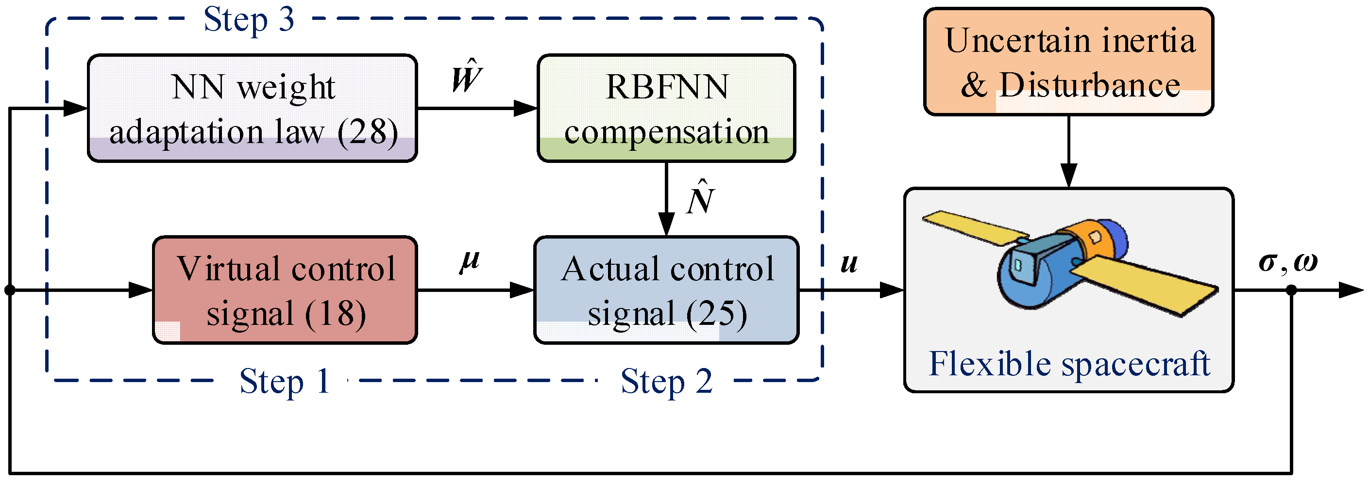
• Rather than the terminal sliding mode control technique, the proposed controller was developed under the fixed-time backstepping control framework. In this way, the proposed controller does not have the chattering phenomenon and singularity problem existing in the terminal sliding mode control.
• The NN was integrated with the proposed controller to compensate the lumped unknown item. Benefiting from the NN compensation, the proposed controller is not only robust against uncertain inertia and external disturbance, but also insensitive to elastic vibrations of the flexible appendages.

The rest of this paper is arranged as follows. Section 2 describes the problem and provides some preliminaries. Section 3 provides the control design and Lyapunov analysis. Section 4 presents the simulations and detailed comparisons. Lastly, Section 5 summarizes this research.

2. Problem Description and Preliminaries

2.1. Problem Description

Suppose a flexible spacecraft composed of a rigid hub and flexible appendages. By employing the modified Rodrigues parameters (MRPs), the attitude kinematics of the flexible spacecraft can be expressed as

$$\dot{\sigma }=G\left(\sigma \right)\omega ,$$

(1)

where $G\left(\sigma \right)=\frac{1}{2}\left(\frac{1-{\sigma }^{\mathrm{T}}\sigma }{2}{\mathbf{I}}_3+{\sigma }^{\times }+\sigma {\sigma }^{\mathrm{T}}\right)\in {ℝ}^{3\times 3}$, $\sigma ={\left[{\sigma }_1,{\sigma }_2,{\sigma }_3\right]}^{\mathrm{T}}\in {ℝ}^3$ and $\omega ={\left[{\omega }_1,{\omega }_2,{\omega }_3\right]}^{\mathrm{T}}\in {ℝ}^3$ denote the attitude and angular velocity of the spacecraft, and ${ℝ}^n$ and ${ℝ}^{n\times m}$ stand for the sets of $n\times 1$ real vectors and $n\times n$ real matrices, respectively. The notation ${\omega }^{\times }$ stands for the skew-symmetric matrix of $\omega$, denoted as

$${\omega }^{\times }=\left[\begin{array}{ccc}0& -{\omega }_3& {\omega }_2\\ {\omega }_3& 0& -{\omega }_1\\ -{\omega }_2& {\omega }_1& 0\end{array}\right].$$

(2)

Referring to [20,21], the attitude dynamics of the flexible spacecraft can be expressed as

$$J\dot{\omega }+{\omega }^{\times }\left(J\omega +\delta \dot{\eta }\right)+\delta \ddot{\eta }=\mathrm{sat}\left(u\right)+d,$$

(3)

$$\ddot{\eta }+C\dot{\eta }+K\eta =-{\delta }^{\mathrm{T}}\omega ,$$

(4)

where $J\in {ℝ}^{3\times 3}$ denotes the inertia matrix which may be fully unknown in some extreme cases, $u\in {ℝ}^3$ is the control torques generated by actuators, $d\in {ℝ}^3$ denotes the external disturbance, $\eta \in {ℝ}^L$ denotes the modal variables, $L$ is the number of elastic modes considered in the control design, $\delta \in {ℝ}^{3\times L}$ is the coupling matrix between the rigid hub and the flexible appendages, $C=\mathrm{diag}\left[2{\xi }_1{\omega }_{n1},2{\xi }_2{\omega }_{n2},\dots ,2{\xi }_N{\omega }_{nL}\right]\in {ℝ}^{L\times L}$ is the damping matrix, $K=\mathrm{diag}\left[{\omega }_{n1}^2,{\omega }_{n2}^2,\dots ,{\omega }_{nL}^2\right]\in {ℝ}^{L\times L}$ is the stiffness matrix, and ${\omega }_{ni}$ and ${\xi }_i$ denote the natural frequencies and damping ratios of the $i$th mode, respectively. Moreover, the saturated control torques can be expressed as $\mathrm{sat}\left(u\right)={\left[\mathrm{sat}\left(u_1\right),\mathrm{sat}\left(u_2\right),\mathrm{sat}\left(u_3\right)\right]}^{\mathrm{T}}$, whose elements are presented as

$$\mathrm{sat}\left(u_i\right)=\{\begin{array}{l}{u}_i,\hspace{0.17em}\hspace{0.17em}\left|u_i\right|\le u_{\mathrm{m}},\hfill \\ \mathrm{sgn}\left(u_i\right)u_{\mathrm{m}},\hspace{0.17em}\hspace{0.17em}\left|u_i\right|>u_{\mathrm{m}},\hfill \end{array}\hspace{0.17em}\hspace{0.17em}i=1,2,3,$$

(5)

where $u_{\mathrm{m}}$ stands for the maximum acceptable input value. Then, the saturated control torques can be rewritten as

$$\mathrm{sat}\left(u\right)=u+u_{\Delta },$$

(6)

where $u_{\Delta }$ denotes the input deviations caused by torque saturation. Subsequently, the attitude kinematics and dynamics of the flexible spacecraft can be rearranged as

$$M\left(\sigma \right)\ddot{\sigma }+C\left(\sigma ,\dot{\sigma }\right)\dot{\sigma }=G^{-\mathrm{T}}\left(\sigma \right)u+\chi ,$$

(7)

where $M\left(\sigma \right)=G^{-\mathrm{T}}\left(\sigma \right)J{G}^{-1}\left(\sigma \right)$, $C\left(\sigma ,\dot{\sigma }\right)=-G^{-\mathrm{T}}\left(\sigma \right)J{G}^{-1}\left(\sigma \right)\dot{G}\left(\sigma \right)G^{-1}\left(\sigma \right)-G^{-\mathrm{T}}\left(\sigma \right){\left(J\omega \right)}^{\times }{G}^{-1}\left(\sigma \right)$, and $\chi =G^{-\mathrm{T}}\left(\sigma \right)\left(-{\omega }^{\times }\delta \dot{\eta }-\delta \ddot{\eta }+d+u_{\Delta }\right)$. According to [37], system (7) has the following fundamental properties.

Property 1.

The matrix$M\left(\sigma \right)$is symmetric and positive definite.

Property 2.

The matrix$\dot{M}\left(\sigma \right)-2C\left(\sigma ,\dot{\sigma }\right)$is skew symmetric.

Property 3.

The matrices$M\left(\sigma \right)$and$C\left(\sigma ,\dot{\sigma }\right)$are bounded with$\underset{\_}{m}{\mathrm{I}}_3\le M\left(\sigma \right)\le \overline{m}{\mathrm{I}}_3$and$\Vert C\left(\sigma ,\dot{\sigma }\right)\Vert \le \overline{c}\Vert \dot{\sigma }\Vert$, where$\underset{\_}{m}$, $\overline{m}$, and$\overline{c}$are positive constants.

The purpose of this research was to develop an appropriate controller to realize the fixed-time attitude stabilization of flexible spacecraft even under uncertain inertia, external disturbance, and torque saturation.

2.2. Preliminaries

The following lemmas are provided, which will be used to obtain the main results of this research.

Lemma 1

([32]). Consider the nonlinear system:

$$\dot{x}=f\left(x\right),\hspace{0.17em}\hspace{0.17em}f\left(0\right)=0,\hspace{0.17em}\hspace{0.17em}x\in {ℝ}^n,$$

(8)

where$f\left(x\right)$is a continuous nonlinear function. If there exists a positive definite function$V\left(x\right)$ satisfying $\dot{V}\left(x\right)\le -{\kappa }_1{V}^p\left(x\right)-{\kappa }_2{V}^q\left(x\right)+\zeta$, where ${\kappa }_1>0$, ${\kappa }_2>0$, $0<p<1$, $q>1$, and $\zeta >0$, then system (8) is practically fixed-time stable, and $V\left(x\right)$ will converge to the following compact set in fixed time:

$$\Omega =\left\{V\left(x\right)\in ℝ|V\left(x\right)\le \min \left\{{\left(\frac{\zeta }{{\kappa }_1\left(1-\iota \right)}\right)}^{\frac{1}{p}},{\left(\frac{\zeta }{{\kappa }_2\left(1-\iota \right)}\right)}^{\frac{1}{q}}\right\}\right\},$$

(9)

where $0<\iota <1$, and the fixed settling time is bounded as $T\le \frac{1}{{\kappa }_1\iota \left(1-p\right)}+\frac{1}{{\kappa }_2\iota \left(q-1\right)}$.

Lemma 2

([38]). For a continuous nonlinear function $f\left(Z\right)$, $Z\in {ℝ}^n$, it can be identified by a radial basis function NN (RBFNN) as

$$f\left(Z\right)=W^{\ast \mathrm{T}}\Phi \left(Z\right)+\epsilon \left(Z\right),$$

(10)

where$W^{\ast }\in {ℝ}^N$is the ideal RBFNN weight,$\Phi \left(Z\right)={\left[{\phi }_1\left(Z\right),{\phi }_2\left(Z\right),\dots ,{\phi }_N\left(Z\right)\right]}^{\mathrm{T}}$is the basis function vector,$\epsilon \left(Z\right)$is the identification error satisfying$\left|\epsilon \left(Z\right)\right|\le \overline{\epsilon }$, $\overline{\epsilon }$is a positive constant, and$N$is the number of RBFNN nodes. The ideal RBFNN weight$W^{\ast }$is defined as

$$W^{\ast }=\arg \underset{W\in {ℝ}^N}{\min }\left\{\underset{Z\in {ℝ}^n}{\sup }\left|f\left(Z\right)-W^{\ast \mathrm{T}}\Phi \left(Z\right)\right|\right\}.$$

(11)

In addition,${\phi }_i\left(Z\right)$is commonly chosen as the Gaussian function:

$${\phi }_i\left(Z\right)=\exp \left(-{\Vert Z-c_i\Vert }^2/w_i^2\right),\hspace{0.17em}\hspace{0.17em}i=1,2,\dots ,N,$$

(12)

where$c_i={\left[c_{i1},c_{i2},\dots ,c_{in}\right]}^{\mathrm{T}}\in {ℝ}^n$and$w_i$are the center and width of the Gaussian function, respectively.

Lemma 3

([39]). For $x_i\in ℝ$, $i=1,2,\dots ,n$, $0<p\le 1$, and $q>1$, the following inequalities hold:

$${\left({\displaystyle \sum _{i=1}^n\left|x_i\right|}\right)}^p\le {\displaystyle \sum _{i=1}^n{\left|x_i\right|}^p},\hspace{0.17em}\hspace{0.17em}{\left({\displaystyle \sum _{i=1}^n\left|x_i\right|}\right)}^q\le n^{q-1}{\displaystyle \sum _{i=1}^n{\left|x_i\right|}^q}.$$

(13)

Lemma 4

([39]). For $x_1\in ℝ$, $x_2\in ℝ$, $p>0$, $q>0$, and $\xi >0$, the following inequality holds:

$${\left|x_1\right|}^p{\left|x_2\right|}^q\le \frac{p}{p+q}\xi {\left|x_1\right|}^{p+q}+\frac{q}{p+q}{\xi }^{-\frac{p}{q}}{\left|x_2\right|}^{p+q}.$$

(14)

3. Control Design and Lyapunov Analysis

In this section, the main results of this research are presented. First, the proposed neural adaptive fixed-time controller is synthesized by embedding the NN compensation into the fixed-time backstepping control framework. Then, the practical fixed-time stability of the overall closed-loop system is theoretically achieved through Lyapunov analysis.

3.1. Control Design

Under the fixed-time backstepping control framework, define the following error signals:

$$x_1=\sigma ,\hspace{0.17em}\hspace{0.17em}{x}_2=\dot{\sigma }-\mu ,$$

(15)

where $\mu \in {ℝ}^3$ is the virtual control signal designed in the sequel. The whole control design procedure involves three steps. In Step 1, the virtual control signal is designed, in Step 2, the actual control signal is designed, and in Step 3, the NN weight adaptation law is designed.

Step 1: Virtual control signal design. Construct the Lyapunov function:

$$V_1=\frac{1}{2}{x}_1^{\mathrm{T}}{x}_1.$$

(16)

The time differentiation of (16) can be evaluated as

$$\begin{array}{l}{\dot{V}}_1=x_1^{\mathrm{T}}{\dot{x}}_1\\ \hspace{0.17em}\hspace{0.17em}\hspace{0.17em}\hspace{0.17em}=x_1^{\mathrm{T}}\left(x_2+\mu \right).\end{array}$$

(17)

Then, the virtual control signal is designed as

$$\mu =-k_{11}{\mathrm{sig}}^p\left(x_1\right)-k_{12}{\mathrm{sig}}^q\left(x_1\right),$$

(18)

where $k_{11}>0$, $k_{12}>0$, $0<p<1$, $q>1$, and the notation ${\mathrm{sig}}^p(\cdot )$ is defined as ${\mathrm{sig}}^p\left(x_1\right)={\left[{\left|x_{11}\right|}^p\mathrm{sgn}\left(x_{11}\right),{\left|x_{12}\right|}^p\mathrm{sgn}\left(x_{12}\right),{\left|x_{13}\right|}^p\mathrm{sgn}\left(x_{13}\right)\right]}^{\mathrm{T}}$. Substituting the virtual control signal (18) into (17) and by the aid of Lemma 3, we have

$$\begin{array}{l}{\dot{V}}_1=x_1^{\mathrm{T}}\left(x_2-k_{11}{\mathrm{sig}}^p\left(x_1\right)-k_{12}{\mathrm{sig}}^q\left(x_1\right)\right)\\ \hspace{0.17em}\hspace{0.17em}\hspace{0.17em}\hspace{0.17em}\le x_1^{\mathrm{T}}{x}_2-{\kappa }_{11}{V}_1^{\frac{p+1}{2}}-{\kappa }_{12}{V}_1^{\frac{q+1}{2}},\end{array}$$

(19)

where ${\kappa }_{11}=2^{\frac{p+1}{2}}{k}_{11}$, and ${\kappa }_{12}=3^{\frac{1-q}{2}}{2}^{\frac{q+1}{2}}{k}_{12}$.

Step 2: Actual control signal design. Construct the Lyapunov function:

$$V_2=\frac{1}{2}{x}_2^{\mathrm{T}}M\left(\sigma \right)x_2.$$

(20)

By the aid of Property 2, the time differentiation of (20) can be evaluated as

$$\begin{array}{l}{\dot{V}}_2=x_2^{\mathrm{T}}M\left(\sigma \right){\dot{x}}_2+\frac{1}{2}{x}_2^{\mathrm{T}}\dot{M}\left(\sigma \right)x_2\\ \hspace{0.17em}\hspace{0.17em}\hspace{0.17em}\hspace{0.17em}=x_2^{\mathrm{T}}\left(-M\left(\sigma \right){\ddot{\sigma }}_{\mathrm{d}}-C\left(\sigma ,\dot{\sigma }\right)\dot{\sigma }+G^{-\mathrm{T}}\left(\sigma \right)u+\chi -M\left(\sigma \right)\dot{\mu }\right)+x_2^{\mathrm{T}}C\left(\sigma ,\dot{\sigma }\right)x_2\\ \hspace{0.17em}\hspace{0.17em}\hspace{0.17em}\hspace{0.17em}=x_2^{\mathrm{T}}\left(-M\left(\sigma \right){\ddot{\sigma }}_{\mathrm{d}}-C\left(\sigma ,\dot{\sigma }\right){\dot{\sigma }}_{\mathrm{d}}-M\left(\sigma \right)\dot{\mu }-C\left(q,\dot{q}\right)\mu +G^{-\mathrm{T}}\left(\sigma \right)u+\chi \right)\\ \hspace{0.17em}\hspace{0.17em}\hspace{0.17em}\hspace{0.17em}=x_2^{\mathrm{T}}\left(G^{-\mathrm{T}}\left(\sigma \right)u+L\right),\end{array}$$

(21)

where $L$ is the lumped unknown term involving uncertain inertia, external disturbance, torque saturation, and elastic vibrations, denoted as

$$L=-M\left(\sigma \right){\ddot{\sigma }}_{\mathrm{d}}-C\left(\sigma ,\dot{\sigma }\right){\dot{\sigma }}_{\mathrm{d}}-M\left(\sigma \right)\dot{\mu }-C\left(q,\dot{q}\right)\mu +\chi .$$

(22)

Define the input variable $Z={\left[x_1^{\mathrm{T}},x_2^{\mathrm{T}},u^{\mathrm{T}}\right]}^{\mathrm{T}}$. The RBFNN is introduced to identify the lumped unknown term. By Lemma 2, the lumped unknown term can be expressed as

$$L=W^{\ast \mathrm{T}}\Phi \left(Z\right)+\epsilon \left(Z\right),$$

(23)

where $W^{\ast }\in {ℝ}^{N\times 3}$ is the ideal RBFNN weight, $\Phi \left(Z\right)\in {ℝ}^N$ is the basis function vector, and $\epsilon \left(Z\right)\in {ℝ}^3$ is the identification error satisfying $\Vert \epsilon \left(Z\right)\Vert \le \overline{\epsilon }$. Subsequently, the lumped unknown term can be identified by the RBFNN as

$$\widehat{L}={\widehat{W}}^{\mathrm{T}}\Phi \left(Z\right),$$

(24)

where $\widehat{W}\in {ℝ}^{N\times 3}$ is the estimation of the ideal RBFNN weight. Then, the actual control signal is designed as

$$u=G^{\mathrm{T}}\left(\sigma \right)\left(-x_1-\frac{1}{2}{x}_2-k_{21}{\mathrm{sig}}^p\left(x_2\right)-k_{22}{\mathrm{sig}}^q\left(x_2\right)-{\widehat{W}}^{\mathrm{T}}\Phi \left(Z\right)\right),$$

(25)

where $k_{11}>0$, and $k_{12}>0$. Substituting the actual control signal (25) into (21), we have

$$\begin{array}{l}{\dot{V}}_2=x_2^{\mathrm{T}}\left(-x_1-\frac{1}{2}{x}_2-k_{21}{\mathrm{sig}}^p\left(x_2\right)-k_{22}{\mathrm{sig}}^q\left(x_2\right)-{\widehat{W}}^{\mathrm{T}}\Phi \left(Z\right)+W^{\ast \mathrm{T}}\Phi \left(Z\right)+\epsilon \left(Z\right)\right)\\ \hspace{0.17em}\hspace{0.17em}\hspace{0.17em}\hspace{0.17em}=x_2^{\mathrm{T}}\left(-x_1-\frac{1}{2}{x}_2-k_{21}{\mathrm{sig}}^p\left(x_2\right)-k_{22}{\mathrm{sig}}^q\left(x_2\right)-{\tilde{W}}^{\mathrm{T}}\Phi \left(Z\right)+\epsilon \left(Z\right)\right),\end{array}$$

(26)

where $\tilde{W}=\widehat{W}-W^{\ast }$ is the estimation error of the RBFNN weight. Consider the inequality $x_2^{\mathrm{T}}\epsilon \left(Z\right)\le \frac{1}{2}{x}_2^{\mathrm{T}}{x}_2+\frac{1}{2}{\overline{\epsilon }}^2$. Substituting it into (26) and by the aid of Lemma 3, we further have

$$\begin{array}{l}{\dot{V}}_2\le -\frac{1}{2}{x}_2^{\mathrm{T}}{x}_1+x_2^{\mathrm{T}}\left(-k_{21}{\mathrm{sig}}^p\left(x_2\right)-k_{22}{\mathrm{sig}}^q\left(x_2\right)\right)-x_2^{\mathrm{T}}{\tilde{W}}^{\mathrm{T}}\Phi \left(Z\right)+\frac{1}{2}{\overline{\epsilon }}^2\\ \hspace{0.17em}\hspace{0.17em}\hspace{0.17em}\hspace{0.17em}\le -\frac{1}{2}{x}_2^{\mathrm{T}}{x}_1-{\kappa }_{21}{V}_2^{\frac{p+1}{2}}-{\kappa }_{22}{V}_2^{\frac{q+1}{2}}-x_2^{\mathrm{T}}{\tilde{W}}^{\mathrm{T}}\Phi \left(Z\right)+\frac{1}{2}{\overline{\epsilon }}^2,\end{array}$$

(27)

where ${\kappa }_{21}=\frac{2^{\frac{p+1}{2}}{k}_{21}}{{\lambda }_{\max }^{\frac{p+1}{2}}\left(M\left(\sigma \right)\right)}$, ${\kappa }_{22}=\frac{3^{\frac{1-q}{2}}{2}^{\frac{q+1}{2}}{k}_{22}}{{\lambda }_{\max }^{\frac{q+1}{2}}\left(M\left(\sigma \right)\right)}$, and the notations ${\lambda }_{\min }(\cdot )$ and ${\lambda }_{\max }(\cdot )$ represent the minimum and maximum eigenvalues of a matrix, respectively.

Step 3: NN weight adaptation law design. The NN weight adaptation law is given as

$${\dot{\widehat{W}}}_i={\Gamma }_i{\Phi }_i\left(Z_i\right)x_{2i}-{\gamma }_i{\Gamma }_i{\widehat{W}}_i,\hspace{0.17em}\hspace{0.17em}i=1,2,3,$$

(28)

where ${\Gamma }_i\in {ℝ}^{N\times N}$ are positive definite matrices, and ${\gamma }_i$ are small positive constants. Construct the Lyapunov function:

$$V_3=\frac{1}{2}{\displaystyle \sum _{i=1}^3{\tilde{W}}_i^{\mathrm{T}}{\Gamma }_i^{-1}{\tilde{W}}_i}.$$

(29)

The time differentiation of (29) can be evaluated as

$$\begin{array}{l}{\dot{V}}_3={\displaystyle \sum _{i=1}^3{\tilde{W}}_i^{\mathrm{T}}{\Gamma }_i^{-1}{\dot{\widehat{W}}}_i}\\ \hspace{0.17em}\hspace{0.17em}\hspace{0.17em}\hspace{0.17em}={\displaystyle \sum _{i=1}^3{\tilde{W}}_i^{\mathrm{T}}{\Phi }_i\left(Z_i\right)x_{2i}}-{\displaystyle \sum _{i=1}^3{\gamma }_i{\tilde{W}}_i^{\mathrm{T}}{\widehat{W}}_i}.\end{array}$$

(30)

Consider the inequality $-{\tilde{W}}_i^{\mathrm{T}}{\widehat{W}}_i=-{\Vert {\tilde{W}}_i\Vert }^2-{\tilde{W}}_i^{\mathrm{T}}{W}_i^{\ast }\le -\frac{1}{2}{\Vert {\tilde{W}}_i\Vert }^2+\frac{1}{2}{\Vert W_i^{\ast }\Vert }^2$. Substituting it into (30), we have

$$\begin{array}{l}{\dot{V}}_3={\displaystyle \sum _{i=1}^3{\tilde{W}}_i^{\mathrm{T}}{\Phi }_i\left(Z_i\right)x_{2i}}-{\displaystyle \sum _{i=1}^3\frac{{\gamma }_i}{2}{\Vert {\tilde{W}}_i\Vert }^2}+{\displaystyle \sum _{i=1}^3\frac{{\gamma }_i}{2}{\Vert W_i^{\ast }\Vert }^2}\\ \hspace{0.17em}\hspace{0.17em}\hspace{0.17em}\hspace{0.17em}={\displaystyle \sum _{i=1}^3{\tilde{W}}_i^{\mathrm{T}}{\Phi }_i\left(Z_i\right)x_{2i}}-{\displaystyle \sum _{i=1}^3{\left(\frac{{\gamma }_i}{4}{\Vert {\tilde{W}}_i\Vert }^2\right)}^{\frac{p+1}{2}}}-{\displaystyle \sum _{i=1}^3{\left(\frac{{\gamma }_i}{4}{\Vert {\tilde{W}}_i\Vert }^2\right)}^{\frac{q+1}{2}}}+{\zeta }_1,\end{array}$$

(31)

where ${\zeta }_1$ is defined as

$${\zeta }_1={\displaystyle \sum _{i=1}^3{\left(\frac{{\gamma }_i}{4}{\Vert {\tilde{W}}_i\Vert }^2\right)}^{\frac{p+1}{2}}}+{\displaystyle \sum _{i=1}^3{\left(\frac{{\gamma }_i}{4}{\Vert {\tilde{W}}_i\Vert }^2\right)}^{\frac{q+1}{2}}}-{\displaystyle \sum _{i=1}^3\frac{{\gamma }_i}{2}{\Vert {\tilde{W}}_i\Vert }^2}+{\displaystyle \sum _{i=1}^3\frac{{\gamma }_i}{2}{\Vert W_i^{\ast }\Vert }^2}.$$

(32)

Then, the following two cases are discussed. For the case of $\frac{{\gamma }_i}{4}{\Vert {\tilde{W}}_i\Vert }^2\ge 1$, we have

$${\left(\frac{{\gamma }_i}{4}{\Vert {\tilde{W}}_i\Vert }^2\right)}^{\frac{p+1}{2}}+{\left(\frac{{\gamma }_i}{4}{\Vert {\tilde{W}}_i\Vert }^2\right)}^{\frac{q+1}{2}}-\frac{{\gamma }_i}{2}{\Vert {\tilde{W}}_i\Vert }^2\le {\left(\frac{{\gamma }_i}{4}{\Vert {\tilde{W}}_i\Vert }^2\right)}^{\frac{q+1}{2}}-\frac{{\gamma }_i}{4}{\Vert {\tilde{W}}_i\Vert }^2.$$

(33)

For the case of $\frac{{\gamma }_i}{4}{\Vert {\tilde{W}}_i\Vert }^2<1$, by the aid of Lemma 4, we have

$$\begin{array}{l}{\left(\frac{{\gamma }_i}{4}{\Vert {\tilde{W}}_i\Vert }^2\right)}^{\frac{p+1}{2}}+{\left(\frac{{\gamma }_i}{4}{\Vert {\tilde{W}}_i\Vert }^2\right)}^{\frac{q+1}{2}}-\frac{{\gamma }_i}{2}{\Vert {\tilde{W}}_i\Vert }^2\le {\left(\frac{{\gamma }_i}{4}{\Vert {\tilde{W}}_i\Vert }^2\right)}^{\frac{p+1}{2}}-\frac{{\gamma }_i}{4}{\Vert {\tilde{W}}_i\Vert }^2\\ \hspace{0.17em}\hspace{0.17em}\hspace{0.17em}\hspace{0.17em}\hspace{0.17em}\hspace{0.17em}\hspace{0.17em}\hspace{0.17em}\hspace{0.17em}\hspace{0.17em}\hspace{0.17em}\hspace{0.17em}\hspace{0.17em}\hspace{0.17em}\hspace{0.17em}\hspace{0.17em}\hspace{0.17em}\hspace{0.17em}\hspace{0.17em}\hspace{0.17em}\hspace{0.17em}\hspace{0.17em}\hspace{0.17em}\hspace{0.17em}\hspace{0.17em}\hspace{0.17em}\hspace{0.17em}\hspace{0.17em}\hspace{0.17em}\hspace{0.17em}\hspace{0.17em}\hspace{0.17em}\hspace{0.17em}\hspace{0.17em}\hspace{0.17em}\hspace{0.17em}\hspace{0.17em}\hspace{0.17em}\hspace{0.17em}\hspace{0.17em}\hspace{0.17em}\hspace{0.17em}\hspace{0.17em}\hspace{0.17em}\hspace{0.17em}\hspace{0.17em}\hspace{0.17em}\hspace{0.17em}\hspace{0.17em}\hspace{0.17em}\hspace{0.17em}\hspace{0.17em}\hspace{0.17em}\hspace{0.17em}\le \left(1-\overline{p}\right){\overline{p}}^{\frac{\overline{p}}{1-\overline{p}}},\end{array}$$

(34)

where $\overline{p}=\frac{p+1}{2}$. Introduce a compact set $\Theta$ such that $\Theta =\left\{\tilde{W}\in {ℝ}^{N\times 3}|\Vert {\tilde{W}}_i\Vert \le {\beta }_i,\hspace{0.17em}\hspace{0.17em}i=1,2,3\right\}$, where ${\beta }_i$ are positive constants. Combining (33) and (34), it follows that

$${\left(\frac{{\gamma }_i}{4}{\Vert {\tilde{W}}_i\Vert }^2\right)}^{\frac{p+1}{2}}+{\left(\frac{{\gamma }_i}{4}{\Vert {\tilde{W}}_i\Vert }^2\right)}^{\frac{q+1}{2}}-\frac{{\gamma }_i}{2}{\Vert {\tilde{W}}_i\Vert }^2\le {\alpha }_i,$$

(35)

where ${\alpha }_i$ is defined as

$${\alpha }_i=\{\begin{array}{l}\left(1-\overline{p}\right){\overline{p}}^{\frac{\overline{p}}{1-\overline{p}}},\hspace{0.17em}\hspace{0.17em}{\beta }_i<\frac{2}{\sqrt{{\gamma }_i}},\hfill \\ {\left(\frac{{\gamma }_i}{4}{\beta }_i^2\right)}^{\frac{q+1}{2}}-\frac{{\gamma }_i}{4}{\beta }_i^2,\hspace{0.17em}\hspace{0.17em}{\beta }_i\ge \frac{2}{\sqrt{{\gamma }_i}}.\hfill \end{array}$$

(36)

Substituting (35) into (31) and by the aid of Lemma 3, we further have

$${\dot{V}}_3\le {\displaystyle \sum _{i=1}^3{\tilde{W}}_i^{\mathrm{T}}{\Phi }_i\left(Z_i\right)x_{2i}}-{\kappa }_{31}{V}_3^{\frac{p+1}{2}}-{\kappa }_{32}{V}_3^{\frac{q+1}{2}}+{\zeta }_2,$$

(37)

where ${\kappa }_{31}=\frac{{\gamma }_i^{\frac{p+1}{2}}}{2^{\frac{p+1}{2}}{\lambda }_{\max }^{\frac{p+1}{2}}\left({\Gamma }_i^{-1}\right)}$, ${\kappa }_{32}=\frac{3^{\frac{1-q}{2}}{\gamma }_i^{\frac{q+1}{2}}}{2^{\frac{q+1}{2}}{\lambda }_{\max }^{\frac{q+1}{2}}\left({\Gamma }_i^{-1}\right)}$, and ${\zeta }_2={\displaystyle \sum _{i=1}^3\left({\alpha }_i+\frac{{\gamma }_i}{2}{\Vert W_i^{\ast }\Vert }^2\right)}$.

3.2. Lyapunov Analysis

After the above preparations, the main theorem of this research can be obtained as follows.

Theorem 1.

Suppose the flexible spacecraft modeled as (1), (3), and (4), then the overall closed-loop system is practically fixed-time stable under the virtual control signal (18), the actual control signal (25), and the NN weight adaptation law (28). Specifically, the closed-loop error signals$x_1$, $x_2$, and $\tilde{W}$will converge to the following compact sets in fixed time:

$${\Omega }_{x_1}=\left\{x_1\in {ℝ}^3|\Vert x_1\Vert \le \sqrt{\psi }\right\},$$

(38)

$${\Omega }_{x_2}=\left\{x_2\in {ℝ}^3|\Vert x_2\Vert \le \sqrt{\frac{\psi }{{\lambda }_{\min }\left(M\left(\sigma \right)\right)}}\right\},$$

(39)

$${\Omega }_{\tilde{W}}=\left\{\tilde{W}\in {ℝ}^{N\times 3}|\Vert {\tilde{W}}_i\Vert \le \sqrt{\frac{\psi }{{\lambda }_{\min }\left({\Gamma }_i^{-1}\right)}},\hspace{0.17em}\hspace{0.17em}i=1,2,3\right\},$$

(40)

where$\psi >0$is defined in the sequel.

Proof. 

Construct the Lyapunov function:

$$V=V_1+V_2+V_3,$$

(41)

where $V_1$, $V_2$, and $V_3$are defined as (15), (19), and (28), respectively. Combining (19), (27), and (37) and by the aid of Lemma 3, the time differentiation of (41) can be evaluated as

$$\begin{array}{l}\dot{V}={\dot{V}}_1+{\dot{V}}_2+{\dot{V}}_3\\ \hspace{0.17em}\hspace{0.17em}\hspace{0.17em}\le -{\kappa }_{11}{V}_1^{\frac{p+1}{2}}-{\kappa }_{12}{V}_1^{\frac{q+1}{2}}-{\kappa }_{21}{V}_2^{\frac{p+1}{2}}-{\kappa }_{22}{V}_2^{\frac{q+1}{2}}+\frac{1}{2}{\overline{\epsilon }}^2-{\kappa }_{31}{V}_3^{\frac{p+1}{2}}-{\kappa }_{32}{V}_3^{\frac{q+1}{2}}+{\zeta }_2\\ \hspace{0.17em}\hspace{0.17em}\hspace{0.17em}\le -{\kappa }_1{V}^{\frac{p+1}{2}}-{\kappa }_2{\dot{V}}^{\frac{q+1}{2}}+{\zeta }_3,\end{array}$$

(42)

where ${\kappa }_1=\min \left\{{\kappa }_{11},{\kappa }_{21},{\kappa }_{31}\right\}$, ${\kappa }_2=3^{\frac{1-q}{2}}\min \left\{{\kappa }_{12},{\kappa }_{22},{\kappa }_{32}\right\}$, and ${\zeta }_3={\zeta }_2+\frac{1}{2}{\overline{\epsilon }}^2$. By Lemma 1, the overall closed-loop system is practically fixed-time stable, and $V$ will converge to the following compact set in fixed time:

$$\Omega =\left\{V\in ℝ|V\le \min \left\{{\left(\frac{{\zeta }_3}{{\kappa }_1\left(1-\iota \right)}\right)}^{\frac{2}{p+1}},{\left(\frac{{\zeta }_3}{{\kappa }_2\left(1-\iota \right)}\right)}^{\frac{2}{q+1}}\right\}\right\},$$

(43)

where $0<\iota <1$. Moreover, the fixed settling time is bounded as $T\le \frac{2}{{\kappa }_1\iota \left(1-p\right)}+\frac{2}{{\kappa }_2\varsigma \left(\iota -1\right)}$. Then, define a variable as

$$\psi =2\min \left\{{\left(\frac{{\zeta }_3}{{\kappa }_1\left(1-\iota \right)}\right)}^{\frac{2}{p+1}},{\left(\frac{{\zeta }_3}{{\kappa }_2\left(1-\iota \right)}\right)}^{\frac{2}{q+1}}\right\}.$$

(44)

Together with the definition of $V$, it follows that

$$x_1^{\mathrm{T}}{x}_1\le \psi ,$$

(45)

$$x_2^{\mathrm{T}}M\left(\sigma \right)x_2\le \psi ,$$

(46)

$${\tilde{W}}_i^{\mathrm{T}}{\Gamma }_i^{-1}{\tilde{W}}_i\le \psi ,\hspace{0.17em}\hspace{0.17em}i=1,2,3.$$

(47)

Thus, the closed-loop error signals $x_1$, $x_2$, and $\tilde{W}$ will converge to the compact sets ${\Omega }_{x_1}$, ${\Omega }_{x_2}$, and ${\Omega }_{\tilde{W}}$ in fixed time, respectively. This further implies that the proposed controller guarantees the stabilization of attitude $\sigma$ and angular velocity $\omega$ to the small neighborhoods of zero in fixed time. Moreover, from (43), the small neighborhoods of zero are adjustable. If we set the parameters $k_{11}$, $k_{12}$, $k_{21}$, and $k_{22}$ as large as desired, the small neighborhoods can be made sufficiently small. This finishes the proof. □

Remark 1.

To make the proposed controller more friendly to the users, a control parameter selection strategy was carried out. The strategy contained three steps. In Step 1, we determined the control parameters$k_{11}$, $k_{12}$, $k_{21}$, and $k_{22}$. Large $k_{11}$, $k_{12}$, $k_{21}$, $k_{22}$can realize a relatively fast convergence rate; however, they may also lead to relatively large control torques at the same time. In Step 2, we determined the control parameters${\Gamma }_i$ and ${\eta }_i$. Large ${\Gamma }_i$and small ${\eta }_i$ can lead to a relatively fast convergence rate; however, they may in turn result in a relatively poor transient response of the controller. In Step 3, we determined the number of RBFNN nodes $N$. A large $N$ can achieve a relatively high approximation accuracy; however, it may also cause a relatively heavy onboard computational burden. Therefore, the control parameters of the proposed controller needed to be carefully tuned by trial and error for better implementations.

Remark 2.

The RBFNN was introduced to identify the lumped unknown term involving uncertain inertia, external disturbance, torque saturation, and elastic vibrations. Benefiting from this design, the proposed controller appeared to be not only robust against uncertain inertia and external disturbance, but also insensitive to elastic vibrations of the flexible appendages. It should be noticed that the RBFNN utilized in this paper can also be replaced by some other approximation tools, such as wavelet NN, recurrent NN, fuzzy NN, and fuzzy logic system.

Remark 3.

The proposed controller was synthesized by embedding the NN compensation into the fixed-time backstepping control framework. To facilitate the readers’ understanding of the whole control design procedure, the structure of the proposed control approach is depicted in Figure 1.

4. Simulations and Comparisons

Simulations were conducted on a flexible spacecraft with two solar panels to validate the proposed control approach. Referring to [34], the inertia matrix of the flexible spacecraft was chosen as

$$J=\left[\begin{array}{ccc}486.7& 14.9& -1.2\\ 14.9& 177.4& -7.3\\ -1.2& -7.3& 404.3\end{array}\right]\hspace{0.17em}\mathrm{kg}\cdot {\mathrm{m}}^2.$$

(48)

The inertia matrix was fully unknown for the control design. Moreover, the first three elastic modes were considered for the flexible spacecraft. The coupling matrix was

$$\delta =\left[\begin{array}{ccc}1& 0.1& 0.1\\ 0.5& 0.1& 0.01\\ -1& 0.3& 0.01\end{array}\right]\hspace{0.17em}{\mathrm{kg}}^{1/2}\cdot {\mathrm{m}/\mathrm{s}}^2.$$

(49)

The natural frequencies were chosen as ${\omega }_{n1}=1.8912$, ${\omega }_{n2}=2.884$, and ${\omega }_{n3}=3.4181$. The damping ratios were chosen as ${\xi }_1=0.01$, ${\xi }_2=0.01$, and ${\xi }_3=0.01$. The external disturbance was

$$d=\left[\begin{array}{c}0.2\cos \left(0.2\pi t\right)-0.1\sin \left(0.4\pi t\right)-0.1\\ 0.3\sin \left(0.2\pi t\right)-0.1\cos \left(0.4\pi t\right)+0.2\\ 0.2\sin \left(0.2\pi t\right)-0.2\sin \left(0.4\pi t\right)-0.3\end{array}\right]\hspace{0.17em}\mathrm{Nm}.$$

(50)

The initial states of the flexible spacecraft were set as $\sigma \left(0\right)={\left[0.04,-0.06,0.08\right]}^{\mathrm{T}}$, $\omega \left(0\right)={\left[0,0,0\right]}^{\mathrm{T}}\hspace{0.17em}\mathrm{rad}/\mathrm{s}$, $\eta \left(0\right)={\left[0,0,0\right]}^{\mathrm{T}}$, and $\dot{\eta }\left(0\right)={\left[0,0,0\right]}^{\mathrm{T}}$. The maximum acceptable input value was $u_{\mathrm{m}}=10\hspace{0.17em}\mathrm{Nm}$.

Besides the proposed neural adaptive fixed-time controller (25), the finite-time PD-like controller in [40] was also implemented for performance comparisons. Based on the homogeneous method, the compared finite-time PD-like controller was designed as

$$u=G^{\mathrm{T}}\left(\sigma \right)\left(-k_p{\mathrm{sig}}^{{\alpha }_1}\left({\sigma }_e\right)-k_d{\mathrm{sig}}^{{\alpha }_2}\left({\dot{\sigma }}_e\right)\right),$$

(51)

where $k_p>0$, $k_d>0$, $0<{\alpha }_1<1$, and ${\alpha }_2=2{\alpha }_1/\left(1+{\alpha }_1\right)$.

The parameters of the proposed neural adaptive fixed-time controller (25) were $k_{11}=0.1$, $k_{12}=0.1$, $k_{21}=800$, $k_{22}=800$, $p=2/3$, $q=4/3$, ${\Gamma }_i=100I_7$, and ${\eta }_i=0.1$. Seven nodes were selected for the hidden layer of the RBFNN. The parameters of the RBFNN were selected as $c_i={\left[-3,-2,-1,0,1,2,3\right]}^{\mathrm{T}}$ and $w_i=6$. The initial values of the NN weight estimations were ${\widehat{W}}_i=0_7$. On the other hand, the parameters of the compared finite-time PD-like controller (51) were $k_p=150$, $k_d=300$, ${\alpha }_1=1/2$, and ${\alpha }_2=2/3$.

The simulation results for the proposed controller are provided in Figure 2, Figure 3, Figure 4, Figure 5 and Figure 6. Specifically, Figure 2 and Figure 3 show the time profiles of the attitude $\sigma$ and the angular velocity $\omega$. The time profile of the modal variables $\eta$ is presented in Figure 4. Figure 5 shows the time profile of the saturated control torques $u$. The norms of the NN weight estimations $\Vert {\widehat{W}}_i\Vert$ are presented in Figure 6. Moreover, the simulation results for the compared PD-like controller are provided in Figure 7, Figure 8, Figure 9 and Figure 10.

As shown in Figure 2 and Figure 3, the proposed controller guaranteed the stabilization of attitude and angular velocity to the small neighborhoods of zero rapidly and exactly. Nevertheless, Figure 7 and Figure 8 shiw that the stabilization performance of the compared PD-like controller was relatively poor due to the presence of a lumped unknown term involving uncertain inertia, external disturbance, torque saturation, and elastic vibrations. Quantitatively, the steady-state attitude accuracy and the steady-state angular velocity accuracy under the proposed controller were $\left|{\sigma }_i\right|<1\times {10}^{-4}$ and $\left|{\omega }_i\right|<3\times {10}^{-4}\mathrm{rad}/\mathrm{s}$, respectively. By contrast, the steady-state attitude accuracy and the steady-state angular velocity accuracy under the compared PD-like controller were $\left|{\sigma }_i\right|<3\times {10}^{-4}$ and $\left|{\omega }_i\right|<8\times {10}^{-4}\mathrm{rad}/\mathrm{s}$, respectively. It was clearly seen that the proposed controller achieved a much higher control accuracy than the compared PD-like controller. In Figure 4, the elastic vibrations of the flexible appendages were damped nearly to zero within $80\hspace{0.17em}\mathrm{s}$ under the proposed controller. However, Figure 9 shows obvious residual vibrations of the flexible appendages under the compared PD-like controller. Figure 5 and Figure 10 show that the control torques under both controllers always remained within the predefined saturation constraints. Moreover, in Figure 6, the NN weight estimations of the proposed controller changed with time smoothly.

Furthermore, some comparisons between the proposed controller and the compared PD-like controller are provided in detail in Figure 11, Figure 12, Figure 13 and Figure 14. Figure 11 and Figure 12 present the norms of the attitude $\sigma$ and angular velocity $\omega$ under both controllers. Moreover, the vibration energy under both controllers are shown in Figure 13, where the vibration energy index is defined as $E_{\eta }=\frac{1}{2}{\eta }^{\mathrm{T}}\eta$. Figure 14 shows the control energy consumption under both controllers, where the control energy consumption index is defined as $E_u=\frac{1}{2}{\displaystyle {\int }_0^t\Vert u\left(\tau \right)\Vert \mathrm{d}\tau }$. In Figure 11, Figure 12, Figure 13 and Figure 14, it is not difficult to find that the proposed controller realized attitude stabilization with higher accuracy than the compared PD-like controller, with less elastic vibration remaining and less control energy consumption. Additionally, it is obvious that the angular velocity tracking under the compared PD-like controller had a relatively large overshoot, which is unexpected in practical implementations.

Consequently, from the simulations and detailed comparisons, the proposed controller appeared able to achieve a superior stabilization performance and better vibration suppression than the compared PD-like controller. This was mainly due to the NN compensation for the lumped unknown term. On the one hand, the robustness of the proposed controller against uncertain inertia and external disturbance was further enhanced. On the other hand, the elastic vibrations of the flexible appendages were significantly suppressed at the same time.

5. Conclusions

In this paper, a novel neural adaptive fixed-time control approach is proposed for the attitude stabilization and vibration suppression of flexible spacecraft. The NN was introduced to identify the lumped unknown term involving uncertain inertia, external disturbance, torque saturation, and elastic vibrations. After that, the proposed controller was developed by integrating with the NN compensation under the fixed-time backstepping control framework. The proposed controller guaranteed the stabilization of attitude and angular velocity to the adjustable small neighborhoods of zero in fixed time through Lyapunov analysis. It should be pointed out that the proposed controller is not only robust against uncertain inertia and external disturbance, but also insensitive to elastic vibrations of the flexible appendages. At last, the simulation results indicated that the proposed control approach was able to achieve an excellent stabilization performance and good vibration suppression.

References

1. Nagashio, T.; Kida, T.; Ohtani, T.; Hamada, Y. Design and implementation of robust symmetric attitude controller for ETS-VIII spacecraft. Control Eng. Pract. 2010, 18, 1440–1451. [Google Scholar] [CrossRef]
2. Nagashio, T.; Kida, T.; Hamada, Y.; Ohtani, T. Robust two-degrees-of-freedom attitude controller design and flight test result for engineering test satellite-VIII spacecraft. IEEE Trans. Control Syst. Technol. 2014, 22, 157–168. [Google Scholar] [CrossRef]
3. Luo, J.; Wei, C.; Dai, H.; Yin, Z.; Wei, X.; Yuan, J. Robust inertia-free attitude takeover control of postcapture combined spacecraft with guaranteed prescribed performance. ISA Trans. 2018, 74, 28–44. [Google Scholar] [CrossRef] [PubMed]
4. Gao, H.; Ma, G.; Lv, Y.; Guo, Y. Forecasting-based data-driven model-free adaptive sliding mode attitude control of combined spacecraft. Aerosp. Sci. Technol. 2019, 86, 364–374. [Google Scholar] [CrossRef]
5. Huang, X.; Duan, G. Fault-tolerant attitude tracking control of combined spacecraft with reaction wheels under prescribed performance. ISA Trans. 2020, 98, 161–172. [Google Scholar] [CrossRef] [PubMed]
6. Liu, Y.; Ma, G.; Lyu, Y.; Wang, P. Neural network-based reinforcement learning control for combined spacecraft attitude tracking maneuvers. Neurocomputing 2022, 484, 67–78. [Google Scholar] [CrossRef]
7. Modi, V.J. Attitude dynamics of satellites with flexible appendages—A brief review. J. Spacecr. Rocket. 1974, 11, 743–751. [Google Scholar] [CrossRef]
8. Likins, P. Spacecraft attitude dynamics and control—A personal perspective on early developments. J. Guid. Control Dyn. 1986, 9, 129–134. [Google Scholar] [CrossRef]
9. Li, H.; Guo, L.; Zhang, Y. An anti-disturbance PD control scheme for attitude control and stabilization of flexible spacecrafts. Nonlinear Dyn. 2012, 67, 2081–2088. [Google Scholar] [CrossRef]
10. Wang, Z.; Wu, Z.; Li, L.; Yuan, J. A composite anti-disturbance control scheme for attitude stabilization and vibration suppression of flexible spacecrafts. J. Vib. Control 2017, 23, 2470–2477. [Google Scholar] [CrossRef]
11. Sun, H.; Hou, L.; Zong, G.; Guo, L. Composite anti-disturbance attitude and vibration control for flexible spacecraft. IET Control Theory Appl. 2017, 11, 2383–2390. [Google Scholar] [CrossRef]
12. Zhu, Y.; Guo, L.; Qiao, J.; Li, W. An enhanced anti-disturbance attitude control law for flexible spacecrafts subject to multiple disturbances. Control Eng. Pract. 2019, 84, 274–283. [Google Scholar] [CrossRef]
13. Singh, S.N.; Zhang, R. Adaptive output feedback control of spacecraft with flexible appendages by modeling error compensation. Acta Astronaut. 2004, 54, 229–243. [Google Scholar] [CrossRef]
14. Maganti, G.B.; Singh, S.N. Simplified adaptive control of an orbiting flexible spacecraft. Acta Astronaut. 2007, 61, 575–589. [Google Scholar] [CrossRef]
15. Guan, P.; Liu, X.-J.; Liu, J.-Z. Adaptive fuzzy sliding mode control for flexible satellite. Eng. Appl. Artif. Intell. 2005, 18, 451–459. [Google Scholar] [CrossRef]
16. Dong, C.; Xu, L.; Chen, Y.; Wang, Q. Networked flexible spacecraft attitude maneuver based on adaptive fuzzy sliding mode control. Acta Astronaut. 2009, 65, 1561–1570. [Google Scholar] [CrossRef]
17. Hu, Q.; Xiao, B. Intelligent proportional-derivation control for flexible spacecraft attitude stabilization with unknown input saturation. Aerosp. Sci. Technol. 2012, 23, 63–74. [Google Scholar] [CrossRef]
18. Sendi, C.; Ayoubi, M.A. Robust-optimal fuzzy model-based control of flexible spacecraft with actuator constraint. J. Dyn. Syst. Meas. Control 2016, 138, 091004. [Google Scholar] [CrossRef]
19. Sendi, C. Attitude control of a flexible spacecraft via fuzzy optimal variance technique. Mathematics 2022, 10, 179. [Google Scholar] [CrossRef]
20. Di Gennaro, S. Active vibration suppression in flexible spacecraft attitude tracking. J. Guid. Control Dyn. 1998, 21, 400–408. [Google Scholar] [CrossRef]
21. Di Gennaro, S. Output stabilization of flexible spacecraft with active vibration suppression. IEEE Trans. Aerosp. Electron. Syst. 2003, 39, 747–759. [Google Scholar] [CrossRef] [Green Version]
22. Hu, Q.; Ma, G. Variable structure control and active vibration suppression of flexible spacecraft during attitude maneuver. Aerosp. Sci. Technol. 2005, 9, 307–317. [Google Scholar] [CrossRef]
23. Azadi, M.; Fazelzadeh, S.A.; Eghtesad, M.; Azadi, E. Vibration suppression and adaptive-robust control of a smart flexible satellite with three axes maneuvering. Acta Astronaut. 2011, 69, 307–322. [Google Scholar] [CrossRef]
24. Azadi, M.; Eghtesad, M.; Fazelzadeh, S.A.; Azadi, E. Dynamics and control of a smart flexible satellite moving in an orbit. Multibody Syst. Dyn. 2015, 35, 1–23. [Google Scholar] [CrossRef]
25. Wu, S.; Radice, G.; Sun, Z. Robust finite-time control for flexible spacecraft attitude maneuver. J. Aerosp. Eng. 2014, 27, 185–190. [Google Scholar] [CrossRef]
26. Yan, R.; Wu, Z. Finite-time attitude stabilization of flexible spacecrafts via reduced-order SMDO and NTSMC. J. Aerosp. Eng. 2018, 31, 04018023. [Google Scholar] [CrossRef]
27. Zhang, X.; Zong, Q.; Dou, L.; Tian, B.; Liu, W. Finite-time attitude maneuvering and vibration suppression of flexible spacecraft. J. Frankl. Inst. 2020, 357, 11604–11628. [Google Scholar] [CrossRef]
28. Hasan, M.N.; Haris, M.; Qin, S. Vibration suppression and fault-tolerant attitude control for flexible spacecraft with actuator faults and malalignments. Aerosp. Sci. Technol. 2022, 120, 107290. [Google Scholar] [CrossRef]
29. Polyakov, A. Nonlinear feedback design for fixed-time stabilization of linear control systems. IEEE Trans. Autom. Control 2012, 57, 2106–2110. [Google Scholar] [CrossRef] [Green Version]
30. Polyakov, A.; Efimov, D.; Perruquetti, W. Finite-time and fixed-time stabilization: Implicit Lyapunov function approach. Automatica 2015, 51, 332–340. [Google Scholar] [CrossRef] [Green Version]
31. Zuo, Z. Nonsingular fixed-time consensus tracking for second-order multi-agent networks. Automatica 2015, 54, 305–309. [Google Scholar] [CrossRef]
32. Jiang, B.; Hu, Q.; Friswell, M.I. Fixed-time attitude control for rigid spacecraft with actuator saturation and faults. IEEE Trans. Control Syst. Technol. 2016, 24, 1892–1898. [Google Scholar] [CrossRef]
33. Cao, L.; Xiao, B.; Golestani, M. Robust fixed-time attitude stabilization control of flexible spacecraft with actuator uncertainty. Nonlinear Dyn. 2020, 100, 2505–2519. [Google Scholar] [CrossRef]
34. Cao, L.; Xiao, B.; Golestani, M.; Ran, D. Faster fixed-time control of flexible spacecraft attitude stabilization. IEEE Trans. Ind. Informat. 2020, 16, 1281–1290. [Google Scholar] [CrossRef]
35. Esmaeilzadeh, S.M.; Golestani, M.; Mobayen, S. Chattering-free fault-tolerant attitude control with fast fixed-time convergence for flexible spacecraft. Int. J. Control Autom. Syst. 2021, 19, 767–776. [Google Scholar] [CrossRef]
36. Golestani, M.; Esmaeilzadeh, S.M.; Mobayen, S. Fixed-time control for high-precision attitude stabilization of flexible spacecraft. Eur. J. Control 2021, 57, 222–231. [Google Scholar] [CrossRef]
37. Spong, M.W.; Hutchinson, S.; Vidyasagar, M. Robot Modeling and Control; John Wiley and Sons: New York, NY, USA, 2006. [Google Scholar]
38. Sanner, R.M.; Slotine, J.-J.E. Gaussian networks for direct adaptive control. IEEE Trans. Neural Netw. 1992, 3, 837–863. [Google Scholar] [CrossRef]
39. Hardy, G.H.; Littlewood, J.E.; Pólya, G. Inequalities; Cambridge University Press: Cambridge, UK, 1952. [Google Scholar]
40. Du, H.; Li, S. Finite-time attitude stabilization for a spacecraft using homogeneous method. J. Guid. Control Dyn. 2012, 35, 740–748. [Google Scholar] [CrossRef]
Figure 1. Diagram of the proposed neural adaptive fixed-time control approach.
Mathematics 10 01667 g001
Figure 2. Time profile of the attitude tracking under the proposed controller.
Mathematics 10 01667 g002
Figure 3. Time profile of the angular velocity tracking under the proposed controller.
Mathematics 10 01667 g003
Figure 4. Time profile of the modal variables under the proposed controller.
Mathematics 10 01667 g004
Figure 5. Time profile of the control torques under the proposed controller.
Mathematics 10 01667 g005
Figure 6. Norms of the NN weight estimations under the proposed controller.
Mathematics 10 01667 g006
Figure 7. Time profile of the attitude tracking under the PD-like controller.
Mathematics 10 01667 g007
Figure 8. Time profile of the angular velocity tracking under the PD-like controller.
Mathematics 10 01667 g008
Figure 9. Time profile of the modal variables under the PD-like controller.
Mathematics 10 01667 g009
Figure 10. Time profile of the control torques under the PD-like controller.
Mathematics 10 01667 g010
Figure 11. Norm of the attitude tracking under both controllers.
Mathematics 10 01667 g011
Figure 12. Norm of the angular velocity tracking under both controllers.
Mathematics 10 01667 g012
Figure 13. Vibration energy under both controllers.
Mathematics 10 01667 g013
Figure 14. Control energy consumption under both controllers.
Mathematics 10 01667 g014
Publisher’s Note: MDPI stays neutral with regard to jurisdictional claims in published maps and institutional affiliations.