
Enhancing Supply Chain Agility with Industry 4.0 Enablers to Mitigate Ripple Effects Based on Integrated QFD-MCDM: An Empirical Study of New Energy Materials Manufacturers


Abstract
:1. Introduction
- (a)
- What are the key REFs, SCAIs, and I4Es in the supply chains of new energy materials manufacturing enterprises?
- (b)
- How must QFD and MCMD be integrated to link the relationships among the three groups of variables and provide decision support for the supply chains of new energy materials manufacturing enterprises?
- (c)
- How can new energy materials manufacturers effectively enhance SCA through I4Es via the proposed framework to mitigate ripple effect?
2. Research Overview
2.1. Ripple Effect Factors (REFs)
2.2. Supply Chain Agility Indicators (SCAIs)
2.3. Industry 4.0 Enablers(I4Es)
2.4. Ripple Effects and Supply Chain Agility
2.5. Supply Chain Agility and Industry 4.0
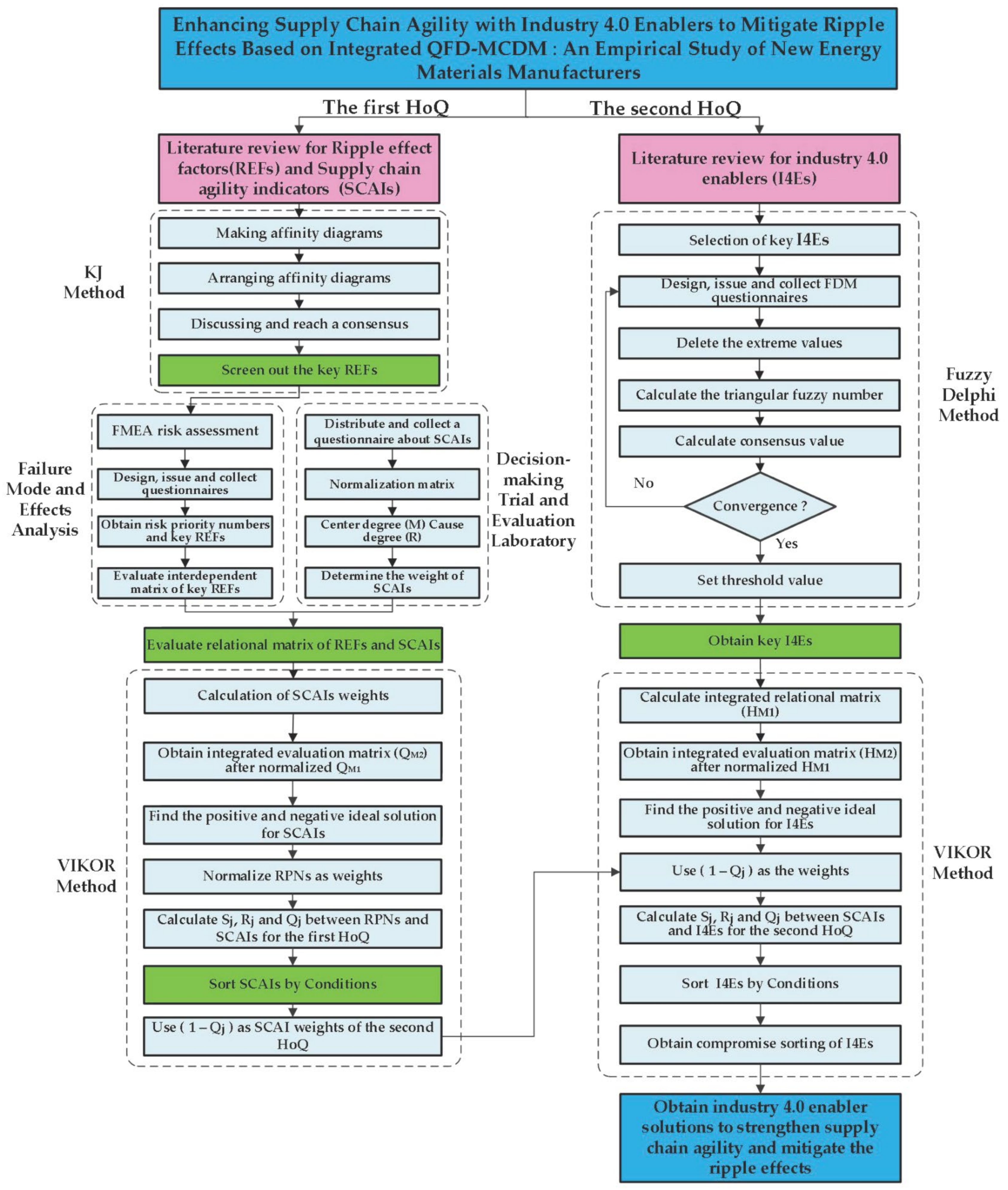
3. Research Method
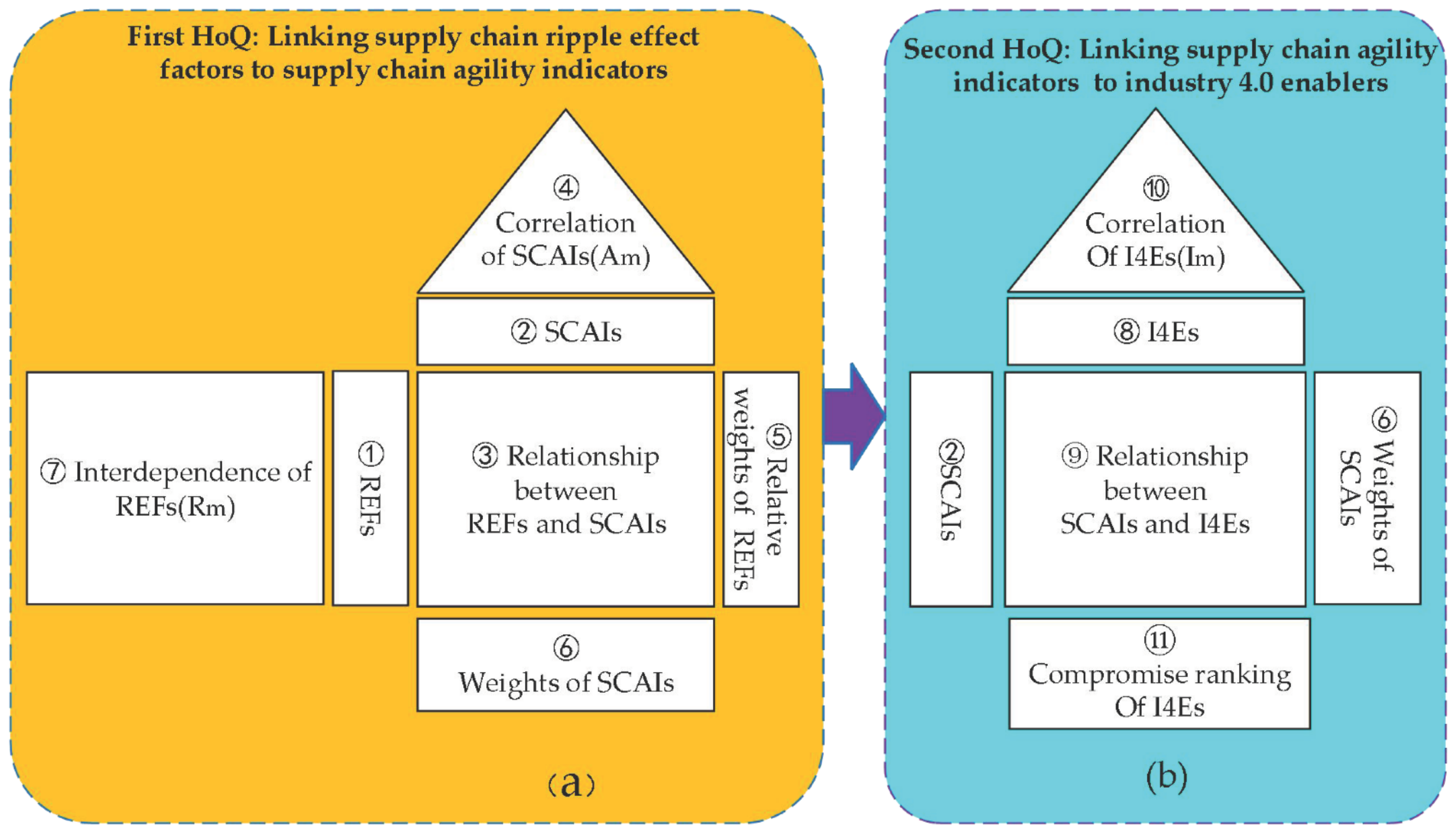
3.1. Research Framework
3.2. First HoQ: Linking REFs to SCAIs
3.3. Second HoQ: Linking SCAIs to I4Es
3.4. KJ Method
- Identify the object (or use): KJ is suitable for problems that need to be solved, but allow sufficient time for the solutions.
- Collect written materials: When collecting materials, it is important to respect facts and seek out original ideas.
- Put all the collected information, including the “original ideas,” on cards.
- Organize the cards.
- 5.
- Gather similar kinds of cards and write down classification cards for each category.
- 6.
- Based on the purpose, select the above data fragments to filter ideas and write articles.
3.5. Failure Mode and Effect Analysis (FMEA)
3.6. Decision-Making Trial and Evaluation Laboratory (DEMATEL)
- The DEMATEL questionnaire was designed for 38 agility indicators collected via literature review and summary, and the degree of influence among the factors was identified according to five scales. The questionnaire results were converted to corresponding values, and the weight value of the influence degree of each factor was obtained after solving the fuzzy average value.
- Based on the influence degree obtained from the questionnaire results, the original relationship matrix Z of the n factors is established, and the diagonal factor Zii of the original relationship matrix is 0.
- The original relation matrix Z is normalized, each row and each column is summed, the maximum value among the row and column summations are determined, and the normalized direct relation matrix Xij is obtained as the matrix normalization.
- The normalized direct relation matrix Xij is used to calculate the total relation influence matrix T.
- By adding the elements in each row and each column in the total influence relation matrix (T), the sum of each column (D value) and sum of each row (R value) is obtained.
- Determination of weight Wi: The weight can be determined as the geometric mean of the centrality and causality, which are obtained by substitutions in Formulas (6) and (7). In this study, the importance order of SCAI was determined according to the calculated weights.
- In the total influence relation matrix T, the sum of all rows and columns is calculated. Further, D + R and D − R are calculated.
3.7. Fuzzy Delphi Method (FDM)
- Step A:
- Identify all I4Es, design the FDM questionnaire for all projects to be evaluated, find and form a suitable expert group, and ask each expert to define a possible range of values for each improvement measure.
- Step B:
- After assessing the questionnaires, calculate the “most conservative cognitive value” and “most optimistic cognitive value” given by the experts, and calculate the minimum, geometric mean, and maximum values of the remaining most conservative cognitive values. Further, the minimum, geometric mean, and maximum of the most optimistic cognitive values are calculated.
- Step C:
- Based on the results of each evaluation item in the second step, each triangle fuzzy number with the most conservative cognitive value and triangle fuzzy number with the most optimistic cognitive value are drawn in their respective double-triangle fuzzy number maps.
- Step D:
- The consensus level Gi is then calculated. Gi refers to the “value importance level for reaching a consensus” as far as the opinions of the experts are concerned. The higher the value of Gi, the greater is the consensus on a particular assessment criterion among the experts. The consensus level is calculated by the following rules:
- (1)
- If the double-triangle fuzzy numbers do not overlap, it indicates that there is consensus on the opinion interval values among the experts. Therefore, the consensus importance value Gi of the evaluation project is equal to the arithmetic average of and :
- (2)
- If two triangular fuzzy numbers overlap, then ( > ) and < , where (), and (). In this case, the “value importance that has reached a consensus” assessment item is calculated using Formula (8).
- (3)
- If two triangular fuzzy numbers overlap, ( > ) and < , which implies conflicts among the experts’ opinions. Thus, steps A to D need to be iterated until convergence is obtained.
- Step E:
- After setting the threshold value of Gi, remove all criteria that did not reach the threshold value.
3.8. VIKOR
4. Empirical Research
4.1. First HoQ: Linking Supply Chain REFs to SCAIs
4.1.1. First Stage: Confirming Important REFs Using the KJ Method
- The main purpose of the KJ method was to identify the REFs of the supply chain of the company in the case study.
- The host of the KJ activity was determined, and six enterprise members were considered for discussion.
- We converted the collected REFs into cards before sorting, classifying, and arranging the cards.
- Through research and discussion, the previously reported 50 REFs of the supply chain were combined and screened for internal affinity, and the 30 possible REFs that are aligned with the actual situation of the company were obtained, as shown in Table 1.
4.1.2. Second Stage: Obtaining Key REFs and RPNs Using FMEA
4.1.3. Third Stage: Using DEMATEL to Screen Key SCAIs
4.1.4. Fourth Stage: Evaluating the Interdependence Matrix between REFs (Rm)
4.1.5. Fifth Stage: Evaluating the Interdependence Matrix among SCAIs (Am)
4.1.6. Sixth Stage: Evaluating the Relationship Matrix between REFs and SCAIs
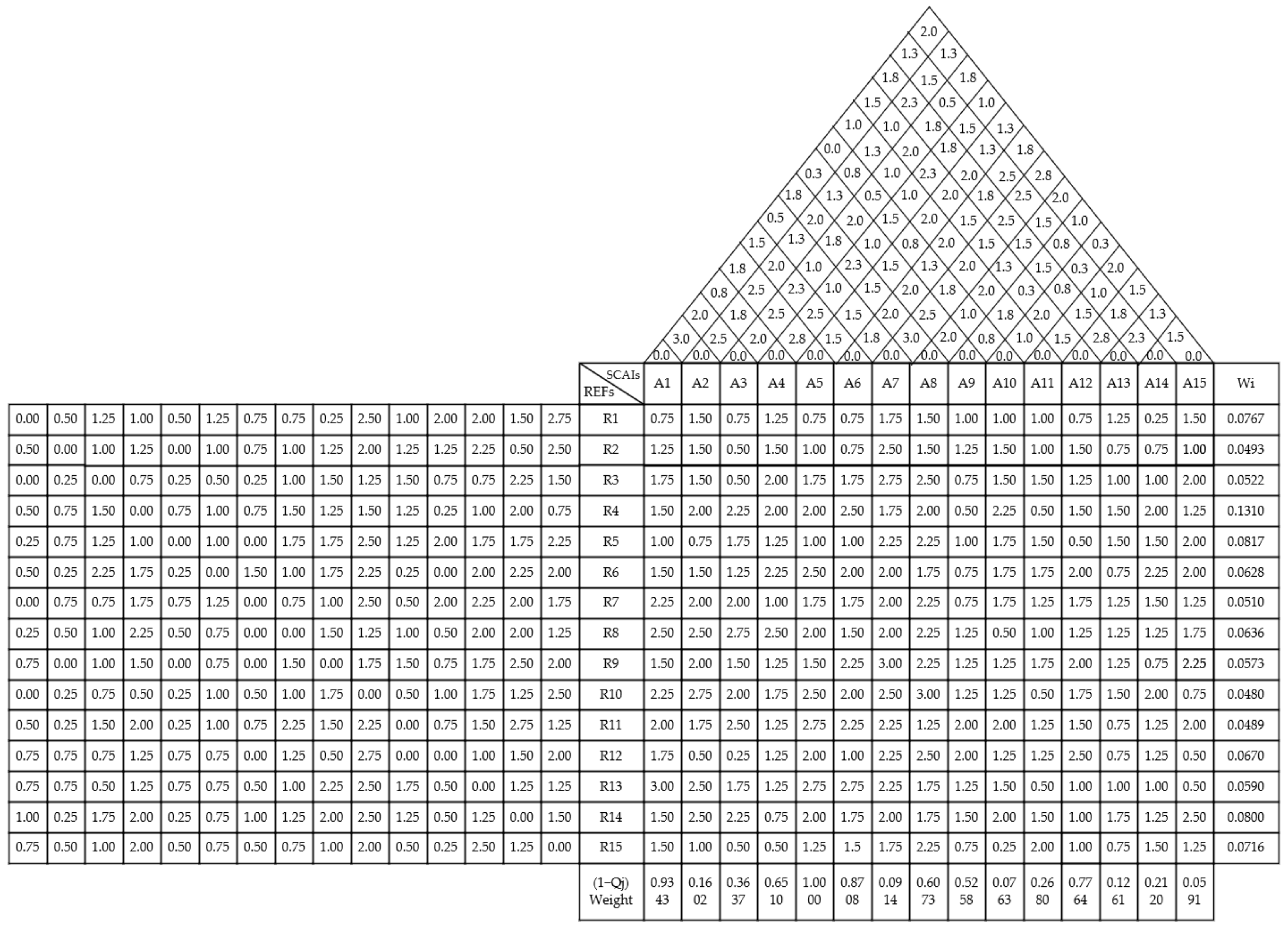
4.1.7. Seventh Stage: Prioritizing Key SCAIs
- Normalize the original data: The initial matrix QM1 is standardized such that the data are within the interval [0, 1] after standardization. The standardized initial matrix QM2 is shown in Table 9.
- Find the positive and negative ideal solutions: The data of the standardized initial matrix QM2 were substituted in Formulas (10) and (11), and the positive ideal solutions and negative ideal solutions of each SCAI were calculated, as shown in Table 10.
- Calculate group utility Sj and individual regret Rj: The RPNs of the REFs obtained by FMEA were standardized, as shown in Table 11.
- D.
- Calculate the benefit ratio Qj: The last step involves calculating the interest ratio Qj. In Formula (14), where v is the decision-making mechanism coefficient. When v > 0.5, it is implied that the final decision is made based on the majority of all the decisions; when v = 0.5, it means that the final decision is made on the basis of approval; when v < 0.5, it means that the final decision is made on the basis of rejection. After careful consideration and discussion, it was decided that v would be set to 0.5 in this study to maximize group utility and minimize individual regret simultaneously. The results calculated according to Formulas (14)–(16) are shown in Table 13. In Formulas (15) and (16), is the maximum group utility, is the minimum individual regret, and the significance of Qj is the profit ratio produced by j schemes. The schemes were sorted according to the results in Table 13. Further, based on the two conditions listed in the methods in Section 3, Qj was substituted into Formula (17). If both conditions are true, the schemes can be sorted by comparing the sizes of Qj (minimum value).
- E.
- Sort SCAIs: Qj belongs to the minimum value index, and the smaller the value is, the better is the index. Therefore, 1 − Qj was taken as the weight of the SCAIs in this study and imported into the second stage of the HoQ. The ranking results of the SCAIs are shown in Table 14 and belong to the HoQ framework in Figure 1 (3). Thus far, the analysis of the first stage of HoQ is complete. Now, the constructed model of the first stage of the HoQ is shown in Figure 3, which is a result of the quality function expansion of the first stage.
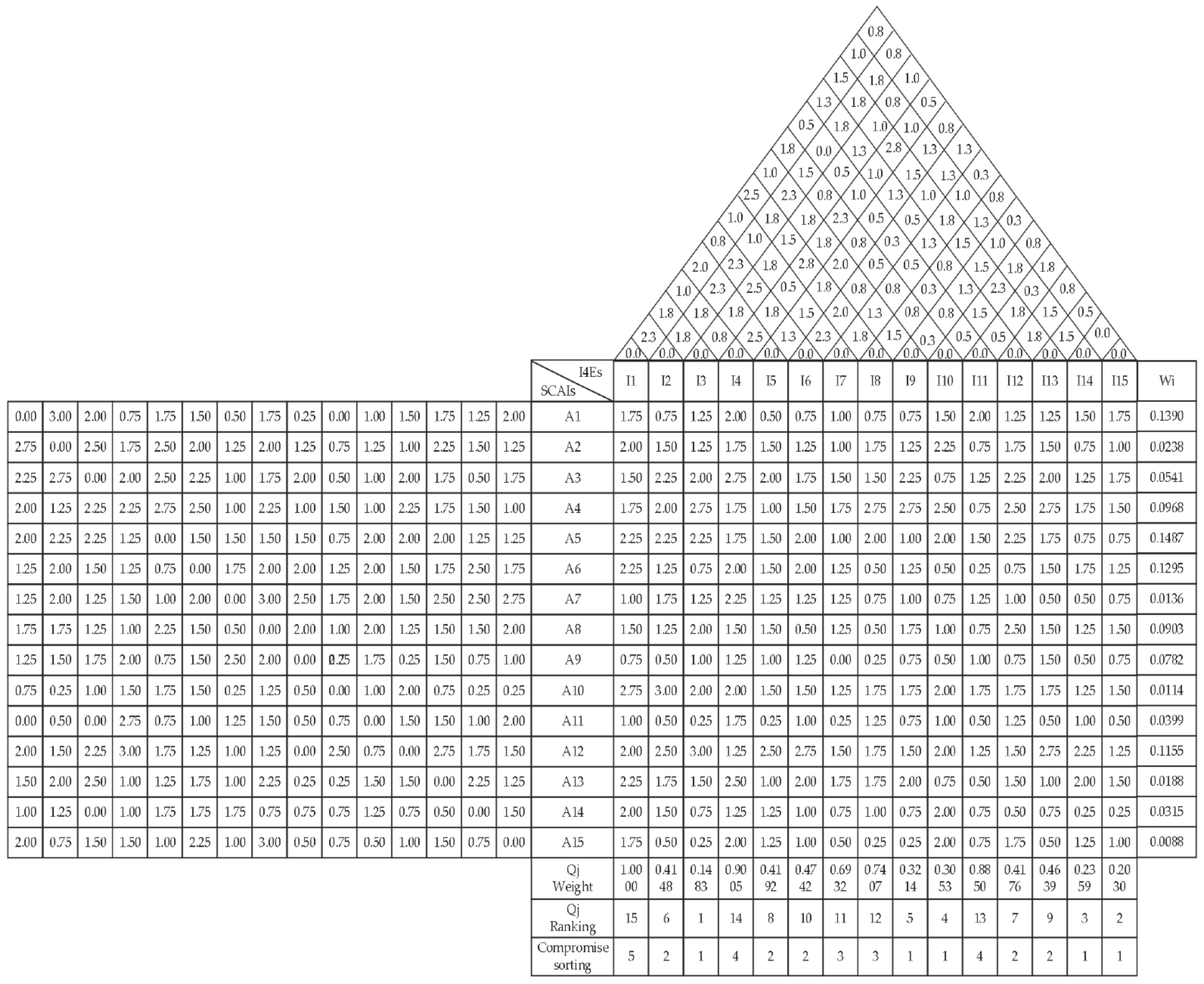
4.2. Second HoQ: Linking SCAIs to I4Es
First Stage: Using FDM to Screen the Index of I4Es
4.3. Results and Discussion
4.3.1. First HoQ: REFs and SCAIs
4.3.2. Second HoQ: SCAIs and I4Es
5. Conclusions
- (1)
- The top three REFs are the bullwhip effect caused by inaccurate predictions, facility failures, and poor strain capacities.
- (2)
- The top three indicators of SCAIs are information transparency and visualization of supply chains to quickly respond to customer needs, long-term cooperation with partners to strengthen trust, and improving customer service levels and satisfaction.
- (3)
- The top five I4Es are ensuring data privacy and security, guarding against legal risks, adopting digital transformation investments to improve economic efficiency, improving IT infrastructure for big data management, and investing in, and using, new Industry 4.0 equipment.
Author Contributions
Funding
Institutional Review Board Statement
Informed Consent Statement
Data Availability Statement
Acknowledgments
Conflicts of Interest
Abbreviations
| REFs | Ripple effect factors |
| SCAIs | Supply chain agility indicators |
| SCA | Supply chain agility |
| I4Es | Industry 4.0 enablers |
| MCDM | Multi-criteria decision making |
| QFD | Quality function deployment |
| HoQ | Houses of quality |
| FMEA | Failure mode and effect analysis |
| DEMATEL | Decision-making Trial and Evaluation Laboratory |
| FDM | Fuzzy Delphi method |
| VIKOR | VlseKriterijumska Optimizacija I Kompromisna Resenje |
Appendix A

| I × I | I1 | I2 | I3 | I4 | I5 | I6 | I7 | I8 | I9 | I10 | I11 | I12 | I13 | I14 | I15 |
|---|---|---|---|---|---|---|---|---|---|---|---|---|---|---|---|
| 1 | 0.00 | 2.25 | 1.75 | 1.00 | 2.00 | 0.75 | 1.00 | 2.50 | 1.00 | 1.75 | 0.50 | 1.25 | 1.50 | 1.00 | 0.75 |
| I2 | 0.75 | 0.00 | 1.75 | 1.75 | 2.25 | 2.25 | 1.00 | 1.75 | 2.25 | 1.50 | 0.00 | 1.75 | 1.75 | 1.75 | 0.75 |
| I3 | 0.75 | 1.25 | 0.00 | 0.75 | 1.75 | 2.50 | 1.75 | 1.50 | 1.75 | 0.75 | 0.50 | 1.25 | 1.00 | 0.75 | 1.00 |
| I4 | 1.50 | 2.75 | 2.00 | 0.00 | 2.50 | 1.75 | 0.50 | 2.75 | 1.75 | 2.25 | 1.00 | 1.00 | 2.75 | 1.00 | 0.50 |
| I5 | 1.25 | 1.75 | 0.25 | 0.75 | 0.00 | 1.25 | 1.50 | 1.75 | 2.00 | 0.75 | 0.50 | 1.25 | 1.50 | 1.25 | 0.75 |
| I6 | 0.25 | 0.50 | 2.50 | 0.50 | 1.25 | 0.00 | 2.25 | 2.00 | 0.75 | 0.50 | 0.25 | 0.50 | 1.00 | 1.25 | 1.25 |
| I7 | 0.50 | 1.00 | 0.50 | 0.75 | 1.50 | 1.50 | 0.00 | 1.75 | 1.25 | 0.75 | 0.50 | 1.25 | 1.75 | 1.00 | 0.25 |
| I8 | 0.50 | 2.50 | 2.75 | 0.75 | 1.50 | 1.00 | 1.25 | 0.00 | 1.50 | 0.75 | 0.25 | 0.75 | 1.50 | 1.25 | 0.75 |
| I9 | 1.00 | 3.00 | 2.00 | 0.25 | 1.00 | 1.00 | 0.25 | 2.25 | 0.00 | 0.25 | 0.75 | 1.25 | 1.50 | 1.00 | 0.25 |
| I10 | 2.00 | 1.25 | 0.50 | 2.00 | 1.75 | 1.50 | 1.75 | 1.25 | 2.25 | 0.00 | 0.50 | 1.50 | 2.25 | 1.75 | 0.75 |
| I11 | 1.25 | 1.00 | 1.50 | 1.00 | 1.75 | 2.00 | 0.50 | 0.75 | 0.75 | 1.25 | 0.00 | 0.50 | 1.75 | 0.25 | 1.75 |
| I12 | 1.50 | 1.50 | 2.25 | 0.25 | 1.00 | 0.25 | 0.00 | 0.75 | 1.50 | 0.50 | 0.50 | 0.00 | 1.75 | 1.50 | 0.75 |
| I13 | 1.00 | 1.50 | 1.75 | 1.75 | 1.75 | 1.75 | 1.50 | 1.00 | 1.25 | 1.25 | 0.50 | 1.50 | 0.00 | 1.50 | 0.50 |
| I14 | 2.75 | 1.25 | 1.25 | 1.50 | 1.00 | 1.50 | 1.50 | 1.50 | 1.00 | 0.25 | 0.75 | 1.25 | 1.75 | 0.00 | 0.00 |
| I15 | 2.25 | 1.00 | 1.75 | 1.50 | 1.25 | 1.25 | 1.00 | 0.75 | 0.75 | 0.50 | 1.75 | 0.50 | 1.00 | 1.25 | 0.00 |
| A × I | I1 | I2 | I3 | I4 | I5 | I6 | I7 | I8 | I9 | I10 | I11 | I12 | I13 | I14 | I15 |
|---|---|---|---|---|---|---|---|---|---|---|---|---|---|---|---|
| A1 | 1.75 | 0.75 | 1.25 | 2.00 | 0.50 | 0.75 | 1.00 | 0.75 | 0.75 | 1.50 | 2.00 | 1.25 | 1.25 | 1.50 | 1.75 |
| A2 | 2.00 | 1.50 | 1.25 | 1.75 | 1.50 | 1.25 | 1.00 | 1.75 | 1.25 | 2.25 | 0.75 | 1.75 | 1.50 | 0.75 | 1.00 |
| A3 | 1.50 | 2.25 | 2.00 | 2.75 | 2.00 | 1.75 | 1.50 | 1.50 | 2.25 | 0.75 | 1.25 | 2.25 | 2.00 | 1.25 | 1.75 |
| A4 | 1.75 | 2.00 | 2.75 | 1.75 | 1.00 | 1.50 | 1.75 | 2.75 | 2.75 | 2.50 | 0.75 | 2.50 | 2.75 | 1.75 | 1.50 |
| A5 | 2.25 | 2.25 | 2.25 | 1.75 | 1.50 | 2.00 | 1.00 | 2.00 | 1.00 | 2.00 | 1.50 | 2.25 | 1.75 | 0.75 | 0.75 |
| A6 | 1.25 | 1.25 | 0.75 | 2.00 | 1.50 | 2.00 | 1.25 | 0.50 | 1.25 | 0.50 | 0.25 | 0.75 | 1.50 | 1.75 | 1.50 |
| A7 | 1.00 | 1.75 | 1.25 | 2.25 | 1.25 | 1.25 | 1.25 | 0.75 | 1.00 | 0.75 | 1.25 | 1.00 | 0.50 | 0.50 | 0.75 |
| A8 | 1.50 | 1.25 | 2.00 | 1.50 | 1.50 | 0.50 | 1.25 | 0.50 | 1.75 | 1.00 | 0.75 | 2.50 | 1.50 | 1.25 | 1.25 |
| A9 | 0.75 | 0.50 | 1.00 | 1.25 | 1.00 | 1.25 | 0.00 | 0.25 | 0.75 | 0.50 | 1.00 | 0.75 | 1.50 | 0.50 | 0.75 |
| A10 | 2.75 | 3.00 | 2.00 | 2.00 | 1.50 | 1.50 | 1.25 | 1.75 | 1.75 | 2.00 | 1.75 | 1.75 | 1.75 | 1.25 | 1.50 |
| A11 | 1.00 | 0.50 | 0.25 | 1.75 | 0.25 | 1.00 | 0.25 | 1.25 | 0.75 | 1.00 | 0.50 | 1.25 | 0.50 | 1.00 | 0.50 |
| A12 | 2.00 | 2.50 | 3.00 | 1.25 | 2.50 | 2.75 | 1.50 | 1.75 | 1.50 | 2.00 | 1.25 | 1.50 | 2.75 | 2.25 | 1.25 |
| A13 | 2.25 | 1.75 | 1.50 | 2.50 | 1.00 | 2.00 | 1.75 | 1.75 | 2.00 | 0.75 | 0.50 | 1.50 | 1.00 | 2.00 | 1.50 |
| A14 | 2.00 | 1.50 | 0.75 | 1.25 | 1.25 | 1.00 | 0.75 | 1.00 | 0.75 | 2.00 | 0.75 | 0.50 | 0.75 | 0.25 | 0.25 |
| A15 | 1.75 | 0.50 | 0.25 | 2.00 | 1.25 | 1.00 | 0.50 | 0.25 | 0.25 | 2.00 | 0.75 | 1.75 | 0.50 | 1.25 | 1.00 |
| HM1 | I1 | I2 | I3 | I4 | I5 | I6 | I7 | I8 | I9 | I10 | I11 | I12 | I13 | I14 | I15 |
|---|---|---|---|---|---|---|---|---|---|---|---|---|---|---|---|
| A1 | 451.20 | 621.52 | 614.31 | 377.83 | 610.00 | 533.39 | 427.72 | 625.72 | 549.16 | 367.02 | 221.88 | 421.69 | 620.83 | 459.23 | 267.03 |
| A2 | 568.03 | 774.67 | 770.66 | 471.22 | 769.42 | 676.45 | 527.78 | 780.64 | 676.38 | 463.89 | 280.23 | 524.11 | 774.03 | 564.45 | 334.39 |
| A3 | 563.08 | 763.38 | 757.69 | 474.28 | 758.61 | 665.92 | 533.67 | 766.53 | 674.48 | 452.17 | 274.89 | 520.70 | 762.00 | 562.36 | 332.67 |
| A4 | 570.13 | 775.94 | 774.42 | 481.27 | 776.31 | 685.39 | 542.09 | 792.73 | 690.00 | 470.86 | 279.72 | 533.98 | 780.61 | 573.86 | 342.20 |
| A5 | 566.36 | 772.77 | 764.64 | 470.36 | 760.97 | 669.98 | 527.75 | 773.53 | 672.36 | 455.64 | 279.09 | 523.05 | 767.56 | 562.70 | 329.02 |
| A6 | 517.81 | 712.91 | 702.95 | 434.89 | 706.44 | 618.63 | 486.92 | 715.66 | 628.14 | 425.13 | 252.77 | 483.23 | 714.89 | 522.94 | 310.50 |
| A7 | 612.63 | 835.39 | 824.63 | 510.78 | 822.55 | 718.94 | 572.64 | 841.70 | 730.89 | 495.00 | 301.08 | 565.61 | 833.70 | 610.73 | 357.83 |
| A8 | 493.52 | 675.33 | 674.92 | 416.45 | 672.94 | 584.34 | 470.05 | 677.80 | 595.59 | 403.55 | 240.66 | 457.81 | 676.97 | 496.94 | 295.91 |
| A9 | 417.41 | 573.00 | 566.72 | 340.70 | 564.45 | 493.94 | 380.08 | 576.52 | 497.83 | 342.09 | 206.91 | 383.58 | 575.38 | 415.41 | 242.83 |
| A10 | 344.75 | 469.42 | 467.88 | 292.36 | 465.06 | 413.53 | 331.34 | 470.00 | 414.78 | 275.00 | 168.39 | 323.36 | 463.13 | 347.48 | 203.80 |
| A11 | 330.59 | 449.53 | 443.27 | 279.25 | 446.06 | 393.39 | 313.92 | 457.33 | 400.25 | 266.06 | 161.56 | 310.31 | 451.98 | 333.05 | 194.66 |
| A12 | 571.22 | 790.13 | 783.80 | 480.59 | 784.30 | 684.64 | 530.92 | 788.36 | 689.16 | 468.92 | 282.06 | 534.42 | 789.61 | 577.55 | 337.25 |
| A13 | 535.52 | 732.91 | 720.45 | 450.25 | 721.91 | 637.98 | 501.59 | 728.78 | 645.58 | 429.36 | 261.59 | 498.92 | 727.53 | 540.53 | 314.66 |
| A14 | 333.63 | 451.67 | 451.03 | 278.27 | 451.36 | 393.72 | 313.30 | 456.81 | 401.13 | 271.36 | 162.48 | 306.88 | 456.64 | 333.22 | 198.17 |
| A15 | 440.08 | 598.11 | 590.44 | 364.64 | 590.17 | 524.84 | 405.64 | 602.41 | 520.19 | 354.61 | 218.38 | 407.03 | 593.00 | 435.50 | 253.94 |
| HM2 | I1 | I2 | I3 | I4 | I5 | I6 | I7 | I8 | I9 | I10 | I11 | I12 | I13 | I14 | I15 |
|---|---|---|---|---|---|---|---|---|---|---|---|---|---|---|---|
| A1 | 0.0039 | 0.0054 | 0.0053 | 0.0033 | 0.0053 | 0.0046 | 0.0037 | 0.0054 | 0.0048 | 0.0032 | 0.0019 | 0.0036 | 0.0054 | 0.0040 | 0.0023 |
| A2 | 0.0049 | 0.0067 | 0.0067 | 0.0041 | 0.0067 | 0.0059 | 0.0046 | 0.0068 | 0.0059 | 0.0040 | 0.0024 | 0.0045 | 0.0067 | 0.0049 | 0.0029 |
| A3 | 0.0049 | 0.0066 | 0.0066 | 0.0041 | 0.0066 | 0.0058 | 0.0046 | 0.0066 | 0.0058 | 0.0039 | 0.0024 | 0.0045 | 0.0066 | 0.0049 | 0.0029 |
| A4 | 0.0049 | 0.0067 | 0.0067 | 0.0042 | 0.0067 | 0.0059 | 0.0047 | 0.0069 | 0.0060 | 0.0041 | 0.0024 | 0.0046 | 0.0068 | 0.0050 | 0.0030 |
| A5 | 0.0049 | 0.0067 | 0.0066 | 0.0041 | 0.0066 | 0.0058 | 0.0046 | 0.0067 | 0.0058 | 0.0039 | 0.0024 | 0.0045 | 0.0066 | 0.0049 | 0.0028 |
| A6 | 0.0045 | 0.0062 | 0.0061 | 0.0038 | 0.0061 | 0.0054 | 0.0042 | 0.0062 | 0.0054 | 0.0037 | 0.0022 | 0.0042 | 0.0062 | 0.0045 | 0.0027 |
| A7 | 0.0053 | 0.0072 | 0.0071 | 0.0044 | 0.0071 | 0.0062 | 0.0050 | 0.0073 | 0.0063 | 0.0043 | 0.0026 | 0.0049 | 0.0072 | 0.0053 | 0.0031 |
| A8 | 0.0043 | 0.0058 | 0.0058 | 0.0036 | 0.0058 | 0.0051 | 0.0041 | 0.0059 | 0.0052 | 0.0035 | 0.0021 | 0.0040 | 0.0059 | 0.0043 | 0.0026 |
| A9 | 0.0036 | 0.0050 | 0.0049 | 0.0029 | 0.0049 | 0.0043 | 0.0033 | 0.0050 | 0.0043 | 0.0030 | 0.0018 | 0.0033 | 0.0050 | 0.0036 | 0.0021 |
| A10 | 0.0030 | 0.0041 | 0.0040 | 0.0025 | 0.0040 | 0.0036 | 0.0029 | 0.0041 | 0.0036 | 0.0024 | 0.0015 | 0.0028 | 0.0040 | 0.0030 | 0.0018 |
| A11 | 0.0029 | 0.0039 | 0.0038 | 0.0024 | 0.0039 | 0.0034 | 0.0027 | 0.0040 | 0.0035 | 0.0023 | 0.0014 | 0.0027 | 0.0039 | 0.0029 | 0.0017 |
| A12 | 0.0049 | 0.0068 | 0.0068 | 0.0042 | 0.0068 | 0.0059 | 0.0046 | 0.0068 | 0.0060 | 0.0041 | 0.0024 | 0.0046 | 0.0068 | 0.0050 | 0.0029 |
| A13 | 0.0046 | 0.0063 | 0.0062 | 0.0039 | 0.0062 | 0.0055 | 0.0043 | 0.0063 | 0.0056 | 0.0037 | 0.0023 | 0.0043 | 0.0063 | 0.0047 | 0.0027 |
| A14 | 0.0029 | 0.0039 | 0.0039 | 0.0024 | 0.0039 | 0.0034 | 0.0027 | 0.0040 | 0.0035 | 0.0023 | 0.0014 | 0.0027 | 0.0039 | 0.0029 | 0.0017 |
| A15 | 0.0038 | 0.0052 | 0.0051 | 0.0032 | 0.0051 | 0.0045 | 0.0035 | 0.0052 | 0.0045 | 0.0031 | 0.0019 | 0.0035 | 0.0051 | 0.0038 | 0.0022 |
| I1 | I2 | I3 | I4 | I5 | I6 | I7 | I8 | I9 | I10 | I11 | I12 | I13 | I14 | I15 | |
|---|---|---|---|---|---|---|---|---|---|---|---|---|---|---|---|
| 0.0053 | 0.0072 | 0.0071 | 0.0044 | 0.0071 | 0.0062 | 0.0050 | 0.0073 | 0.0063 | 0.0043 | 0.0026 | 0.0049 | 0.0072 | 0.0053 | 0.0031 | |
| 0.0029 | 0.0039 | 0.0038 | 0.0024 | 0.0039 | 0.0034 | 0.0027 | 0.0040 | 0.0035 | 0.0023 | 0.0014 | 0.0027 | 0.0039 | 0.0029 | 0.0017 |
| SCAIs | A1 | A2 | A3 | A4 | A5 | A6 | A7 | A8 | A9 | A10 | A11 | A12 | A13 | A14 | A15 |
|---|---|---|---|---|---|---|---|---|---|---|---|---|---|---|---|
| Ranking | 2 | 11 | 8 | 5 | 1 | 3 | 13 | 6 | 7 | 14 | 9 | 4 | 12 | 10 | 15 |
| Weight | 0.1390 | 0.0238 | 0.0541 | 0.0968 | 0.1487 | 0.1295 | 0.0136 | 0.0903 | 0.0782 | 0.0114 | 0.0399 | 0.1155 | 0.0188 | 0.0315 | 0.0088 |
| SCAIs | I4Es | |||||||||||||||
|---|---|---|---|---|---|---|---|---|---|---|---|---|---|---|---|---|
| I1 | I2 | I3 | I4 | I5 | I6 | I7 | I8 | I9 | I10 | I11 | I12 | I13 | I14 | I15 | ||
| A1 | 0.1390 | 0.0795 | 0.0770 | 0.0766 | 0.0795 | 0.0785 | 0.0792 | 0.0777 | 0.0780 | 0.0764 | 0.0777 | 0.0789 | 0.0773 | 0.0775 | 0.0758 | 0.0773 |
| A2 | 0.0238 | 0.0038 | 0.0037 | 0.0034 | 0.0041 | 0.0034 | 0.0031 | 0.0041 | 0.0038 | 0.0039 | 0.0032 | 0.0036 | 0.0038 | 0.0037 | 0.0040 | 0.0034 |
| A3 | 0.0541 | 0.0095 | 0.0101 | 0.0095 | 0.0085 | 0.0092 | 0.0088 | 0.0081 | 0.0106 | 0.0092 | 0.0101 | 0.0102 | 0.0094 | 0.0102 | 0.0094 | 0.0083 |
| A4 | 0.0968 | 0.0146 | 0.0149 | 0.0127 | 0.0123 | 0.0119 | 0.0100 | 0.0114 | 0.0123 | 0.0120 | 0.0102 | 0.0148 | 0.0118 | 0.0135 | 0.0129 | 0.0093 |
| A5 | 0.1487 | 0.0244 | 0.0241 | 0.0234 | 0.0259 | 0.0243 | 0.0224 | 0.0257 | 0.0263 | 0.0263 | 0.0256 | 0.0234 | 0.0245 | 0.0258 | 0.0257 | 0.0263 |
| A6 | 0.1295 | 0.0435 | 0.0411 | 0.0413 | 0.0423 | 0.0399 | 0.0399 | 0.0428 | 0.0424 | 0.0403 | 0.0395 | 0.0449 | 0.0412 | 0.0403 | 0.0410 | 0.0376 |
| A7 | 0.0136 | 0.0000 | 0.0000 | 0.0000 | 0.0000 | 0.0000 | 0.0000 | 0.0000 | 0.0000 | 0.0000 | 0.0000 | 0.0000 | 0.0000 | 0.0000 | 0.0000 | 0.0000 |
| A8 | 0.0903 | 0.0382 | 0.0375 | 0.0355 | 0.0366 | 0.0359 | 0.0373 | 0.0357 | 0.0385 | 0.0370 | 0.0361 | 0.0391 | 0.0376 | 0.0371 | 0.0370 | 0.0343 |
| A9 | 0.0782 | 0.0541 | 0.0532 | 0.0529 | 0.0572 | 0.0536 | 0.0541 | 0.0581 | 0.0539 | 0.0551 | 0.0522 | 0.0528 | 0.0550 | 0.0529 | 0.0550 | 0.0551 |
| A10 | 0.0114 | 0.0108 | 0.0108 | 0.0106 | 0.0107 | 0.0108 | 0.0107 | 0.0106 | 0.0110 | 0.0109 | 0.0109 | 0.0108 | 0.0106 | 0.0110 | 0.0108 | 0.0107 |
| A11 | 0.0399 | 0.0399 | 0.0399 | 0.0399 | 0.0397 | 0.0399 | 0.0399 | 0.0398 | 0.0398 | 0.0399 | 0.0399 | 0.0399 | 0.0393 | 0.0399 | 0.0399 | 0.0399 |
| A12 | 0.1155 | 0.0170 | 0.0135 | 0.0124 | 0.0150 | 0.0117 | 0.0122 | 0.0186 | 0.0160 | 0.0146 | 0.0132 | 0.0157 | 0.0139 | 0.0133 | 0.0138 | 0.0146 |
| A13 | 0.0188 | 0.0051 | 0.0050 | 0.0051 | 0.0049 | 0.0050 | 0.0047 | 0.0051 | 0.0055 | 0.0048 | 0.0054 | 0.0053 | 0.0048 | 0.0052 | 0.0047 | 0.0050 |
| A14 | 0.0315 | 0.0312 | 0.0314 | 0.0309 | 0.0315 | 0.0311 | 0.0315 | 0.0315 | 0.0315 | 0.0315 | 0.0308 | 0.0313 | 0.0315 | 0.0312 | 0.0315 | 0.0309 |
| A15 | 0.0088 | 0.0054 | 0.0054 | 0.0054 | 0.0055 | 0.0054 | 0.0053 | 0.0057 | 0.0055 | 0.0056 | 0.0054 | 0.0052 | 0.0054 | 0.0056 | 0.0056 | 0.0056 |
| Sj | — | 0.3770 | 0.3677 | 0.3596 | 0.3736 | 0.3606 | 0.3589 | 0.3750 | 0.3751 | 0.3674 | 0.3602 | 0.3759 | 0.3664 | 0.3671 | 0.3671 | 0.3582 |
| Rj | — | 0.0795 | 0.0770 | 0.0766 | 0.0795 | 0.0785 | 0.0792 | 0.0777 | 0.0780 | 0.0764 | 0.0777 | 0.0789 | 0.0773 | 0.0775 | 0.0758 | 0.0773 |
| I4Es | |||||||||||||||
|---|---|---|---|---|---|---|---|---|---|---|---|---|---|---|---|
| I1 | I2 | I3 | I4 | I5 | I6 | I7 | I8 | I9 | I10 | I11 | I12 | I13 | I14 | I15 | |
| Qj | 1.0000 | 0.4148 | 0.1483 | 0.9005 | 0.4192 | 0.4742 | 0.6932 | 0.7407 | 0.3214 | 0.3053 | 0.8850 | 0.4176 | 0.4639 | 0.2359 | 0.2030 |
References
- Haleem, F.; Farooq, S.; Wæhrens, B.V.; Boer, H. Offshoring experience and performance: The role of realized drivers and risk management. Supply Chain Manag. 2018, 23, 531–544. [Google Scholar] [CrossRef]
- Wiengarten, F.; Humphreys, P.; Gimenez, C.; McIvor, R. Risk, risk management practices, and the success of supply chain integration. Int. J. Prod. Econ. 2016, 171, 361–370. [Google Scholar] [CrossRef]
- Blome, C.; Schoenherr, T. Supply chain risk management in financial crises—A multiple case-study approach. Int. J. Prod. Econ. 2011, 134, 43–57. [Google Scholar] [CrossRef]
- Kauppi, K.; Longoni, A.; Caniato, F.; Kuula, M. Managing country disruption risks and improving operational performance: Risk management along integrated supply chains. Int. J. Prod. Econ. 2016, 182, 484–495. [Google Scholar] [CrossRef]
- Munir, M.; Jajja, M.S.S.; Chatha, K.A.; Farooq, S. Supply chain risk management and operational performance: The enabling role of supply chain integration. Int. J. Prod. Econ. 2020, 227, 107667. [Google Scholar] [CrossRef]
- Shao, L.; Jin, S. Resilience assessment of the lithium supply chain in China under impact of new energy vehicles and supply interruption. J. Clean. Prod. 2020, 252, 119624. [Google Scholar] [CrossRef]
- Ivanov, D. Simulation-based ripple effect modelling in the supply chain. Int. J. Prod. Res. 2017, 55, 2083–2101. [Google Scholar] [CrossRef]
- Ivanov, D.; Sokolov, B.; Dolgui, A. The ripple effect in supply chains: Trade-off ‘efficiency-flexibility-resilience’ in disruption management. Int. J. Prod. Res. 2014, 52, 2154–2172. [Google Scholar] [CrossRef]
- Dolgui, A.; Ivanov, D. Ripple effect and supply chain disruption management: New trends and research directions. Int. J. Prod. Res. 2021, 59, 102–109. [Google Scholar] [CrossRef]
- Ivanov, D.; Dolgui, A.; Das, A.; Sokolov, B. Digital supply chain twins: Managing the ripple effect, resilience, and disruption risks by data-driven optimization, simulation, and visibility. In Handbook of Ripple Effects in the Supply Chain; Springer: Cham, Switzerland, 2019; pp. 309–332. [Google Scholar]
- Shaheen, I.; Azadegan, A.; Hooker, R.; Lucianetti, L. Leadership for mitigating ripple effects in supply chain disruptions: A paradoxical role. In Handbook of Ripple Effects in the Supply Chain; Springer: Cham, Switzerland, 2019; pp. 101–128. [Google Scholar]
- Birkie, S.E.; Trucco, P. Do not expect others do what you should! Supply chain complexity and mitigation of the ripple effect of disruptions. Int. J. Logist. Manag. 2020, 31, 123–144. [Google Scholar] [CrossRef]
- Monostori, J. Mitigation of the ripple effect in supply chains: Balancing the aspects of robustness, complexity and efficiency. CIRP J. Manuf. Sci. Technol. 2021, 32, 370–381. [Google Scholar] [CrossRef]
- Ivanov, D.; Dolgui, A.; Sokolov, B. Supply chain design with disruption considerations: Review of research streams on the ripple effect in the supply chain. IFAC-PapersOnLine 2015, 48, 1700–1707. [Google Scholar] [CrossRef]
- Dolgui, A.; Ivanov, D.; Sokolov, B. Ripple effect in the supply chain: An analysis and recent literature. Int. J. Prod. Res. 2018, 56, 414–430. [Google Scholar] [CrossRef] [Green Version]
- Liu, J.G.; Zhou, Y.X.; Lu, B.; Zhao, J. The reduction mechanism of supply chain vulnerability based on supply chain disruption risk. Syst. Eng.-Theory Pract. 2015, 3, 556–566. [Google Scholar]
- Chiang, C.Y.; Kocabasoglu-Hillmer, C.; Suresh, N. An empirical investigation of the impact of strategic sourcing and flexibility on firm’s supply chain agility. Int. J. Oper. Prod. Manag. 2012, 32, 49–78. [Google Scholar] [CrossRef]
- Giannakis, M.; Louis, M. A multi-agent based system with big data processing for enhanced supply chain agility. J. Enterp. Inf. Manag. 2016, 29, 706–727. [Google Scholar] [CrossRef]
- Agarwal, A.; Shankar, R.; Tiwari, M.K. Modeling agility of supply chain. Ind. Mark. Manag. 2007, 36, 443–457. [Google Scholar] [CrossRef]
- Aslam, H.; Blome, C.; Roscoe, S.; Azhar, T.M. Dynamic supply chain capabilities: How market sensing, supply chain agility and adaptability affect supply chain ambidexterity. Int. J. Oper. Prod. Manag. 2018, 38, 2266–2285. [Google Scholar] [CrossRef]
- Al-Shboul, M.A. Infrastructure framework and manufacturing supply chain agility: The role of delivery dependability and time to market. Supply Chain Manag. Int. J. 2017, 22, 172–185. [Google Scholar] [CrossRef]
- Braunscheidel, M.J.; Suresh, N.C. The organizational antecedents of a firm’s supply chain agility for risk mitigation and response. J. Oper. Manag. 2009, 27, 119–140. [Google Scholar] [CrossRef]
- Swafford, P.M.; Ghosh, S.; Murthy, N. Achieving supply chain agility through IT integration and flexibility. Int. J. Prod. Econ. 2008, 116, 288–297. [Google Scholar] [CrossRef]
- Dubey, R.; Altay, N.; Gunasekaran, A.; Papadopoulos, T.; Childe, S.J. Supply chain agility, adaptability and alignment: Empirical evidence from the Indian auto components industry. Int. J. Oper. Prod. Manag. 2018, 38, 129–148. [Google Scholar] [CrossRef]
- Swafford, P.M.; Ghosh, S.; Murthy, N. The antecedents of supply chain agility of a firm: Scale development and model testing. J. Oper. Manag. 2006, 24, 170–188. [Google Scholar] [CrossRef]
- Mason, S.J.; Cole, M.H.; Ulrey, B.T.; Yan, L. Improving electronics manufacturing supply chain agility through outsourcing. Int. J. Phys. Distrib. Logist. Manag. 2002, 32, 610–620. [Google Scholar] [CrossRef] [Green Version]
- Collin, J.; Lorenzin, D. Plan for supply chain agility at nokia: Lessons from the mobile infrastructure industry. Int. J. Phys. Distrib. Logist. Manag. 2006, 36, 418–430. [Google Scholar] [CrossRef]
- DeGroote, S.E.; Marx, T.G. The impact of IT on supply chain agility and firm performance: An empirical investigation. Int. J. Inf. Manag. 2013, 33, 909–916. [Google Scholar] [CrossRef]
- Gligor, D.; Gligor, N.; Holcomb, M.; Bozkurt, S. Distinguishing between the concepts of supply chain agility and resilience: A multidisciplinary literature review. Int. J. Logist. Manag. 2019, 30, 467–487. [Google Scholar] [CrossRef]
- Panitsettakorn, W.; Ongkunaruk, P. The improvement of supply chain agility during COVID-19: A case study of alcohol sanitizer in Thailand. In Proceedings of the 2021 IEEE 8th International Conference on Industrial Engineering and Applications (ICIEA), Chengdu, China, 23–26 April 2021; IEEE: Piscataway, NJ, USA, 2021; pp. 417–421. [Google Scholar]
- Singh, R.K.; Kumar, P.; Chand, M. Evaluation of supply chain coordination index in context to Industry 4.0 environment. Benchmarking Int. J. 2019, 28, 1622–1637. [Google Scholar] [CrossRef]
- Ghadge, A.; Kara, M.E.; Moradlou, H.; Goswami, M. The impact of Industry 4.0 implementation on supply chains. J. Manuf. Technol. Manag. 2020, 31, 669–686. [Google Scholar] [CrossRef]
- Saengchai, S.; Jermsittiparsert, K. Coping strategy to counter the challenges towards implementation of industry 4.0 in Thailand: Role of supply chain agility and resilience. Int. J. Supply Chain Manag. 2019, 8, 733–744. [Google Scholar]
- Urnau, J.F.; Junior, O.C. Discussion of new product development process sustainability based on the supply chain in the context of industry 4.0. In Integrating Social Responsibility and Sustainable Development: Addressing Challenges and Creating Opportunities; Springer: Cham, Switzerland, 2021; p. 151. [Google Scholar]
- Tjahjono, B.; Esplugues, C.; Ares, E.; Pelaez, G. What does industry 4.0 mean to supply chain? Procedia Manuf. 2017, 13, 1175–1182. [Google Scholar] [CrossRef]
- Fazili, M.; Venkatadri, U.; Cyrus, P.; Tajbakhsh, M. Physical internet, conventional and hybrid logistic systems: A routing optimisation-based comparison using the Eastern Canada road network case study. Int. J. Prod. Res. 2017, 55, 2703–2730. [Google Scholar] [CrossRef]
- Liao, Y.; Deschamps, F.; Loures, E.F.R.; Ramos, L.F.P. Past, present and future of Industry 4.0—A systematic literature review and research agenda proposal. Int. J. Prod. Res. 2017, 55, 3609–3629. [Google Scholar] [CrossRef]
- Qu, T.; Thürer, M.; Wang, J.; Wang, Z.Z.; Fu, H.; Li, C.D.; Huang, G.Q. System dynamics analysis for an internet-of-things-enabled production logistics system. Int. J. Prod. Res. 2017, 55, 2622–2649. [Google Scholar] [CrossRef]
- Castelo-Branco, I.; Cruz-Jesus, F.; Oliveira, T. Assessing industry 4.0 readiness in manufacturing: Evidence for the European union. Comput. Ind. 2019, 107, 22–32. [Google Scholar] [CrossRef]
- Pfeifer, A. An Appraisal of IT Requirements in the Context of Industry 4.0 and of Organizational Agility. Master’s Thesis, Johannes Kepler University Linz, Linz, Austria, 2015. [Google Scholar]
- Rane, S.B.; Narvel, Y.A.M. Re-designing the business organization using disruptive innovations based on blockchain-IoT integrated architecture for improving agility in future Industry 4.0. Benchmarking Int. J. 2019, 28, 1883–1908. [Google Scholar] [CrossRef]
- Lavinsaa, P.; Somu, H.; Ahmad, N.H.; Joshi, J.P.; Wahid, N.A. Industry 4.0 technology re-engineering impacts on strategy agility and SME competitiveness in Malaysia. In Proceedings of the First ASEAN Business, Environment, and Technology Symposium (ABEATS 2019), Bogor, Indonesia, 2–3 December 2019; Atlantis Press: Paris, France, 2020; pp. 52–55. [Google Scholar]
- Eslami, M.H.; Jafari, H.; Achtenhagen, L.; Carlbäck, J.; Wong, A. Financial performance and supply chain dynamic capabilities: The moderating role of industry 4.0 technologies. Int. J. Prod. Res. 2021, 1–18. Available online: https://www.tandfonline.com/doi/full/10.1080/00207543.2021.1966850 (accessed on 3 March 2022). [CrossRef]
- Li, M.; Jin, L.; Wang, J. A new MCDM method combining QFD with TOPSIS for knowledge management system selection from the user’s perspective in intuitionistic fuzzy environment. Appl. Soft Comput. 2014, 21, 28–37. [Google Scholar] [CrossRef]
- Ignatius, J.; Rahman, A.; Yazdani, M.; Šaparauskas, J.; Haron, S.H. An integrated fuzzy ANP–QFD approach for green building assessment. J. Civ. Eng. Manag. 2016, 22, 551–563. [Google Scholar] [CrossRef] [Green Version]
- Tian, Z.; Wang, J.; Wang, J.; Zhang, H. A multi-phase QFD-based hybrid fuzzy MCDM approach for performance evaluation: A case of smart bike-sharing programs in Changsha. J. Clean. Prod. 2018, 171, 1068–1083. [Google Scholar] [CrossRef]
- Wang, X.; Fang, H.; Song, W. Technical attribute prioritisation in QFD based on cloud model and grey relational analysis. Int. J. Prod. Res. 2020, 58, 5751–5768. [Google Scholar] [CrossRef]
- Levner, E.; Ptuskin, A. Entropy-based model for the ripple effect: Managing environmental risks in supply chains. Int. J. Prod. Res. 2018, 56, 2539–2551. [Google Scholar] [CrossRef]
- Hosseini, S.; Ivanov, D.; Dolgui, A. Review of quantitative methods for supply chain resilience analysis. Transp. Res. Part E Logist. Transp. Rev. 2019, 125, 285–307. [Google Scholar] [CrossRef]
- Dolgui, A.; Ivanov, D.; Rozhkov, M. Does the ripple effect influence the bullwhip effect? An integrated analysis of structural and operational dynamics in the supply chain. Int. J. Prod. Res. 2020, 58, 1285–1301. [Google Scholar] [CrossRef]
- Ivanov, D.; Pavlov, A.; Sokolov, B. Optimal distribution (re) planning in a centralized multi-stage supply network under conditions of the ripple effect and structure dynamics. Eur. J. Oper. Res. 2014, 237, 758–770. [Google Scholar] [CrossRef]
- Ivanov, D.; Dolgui, A.; Sokolov, B. The impact of digital technology and Industry 4.0 on the ripple effect and supply chain risk analytics. Int. J. Prod. Res. 2019, 57, 829–846. [Google Scholar] [CrossRef]
- Hosseini, S.; Ivanov, D. Bayesian networks for supply chain risk, resilience and ripple effect analysis: A literature review. Expert Syst. Appl. 2020, 161, 113649. [Google Scholar] [CrossRef]
- Hosseini, S.; Ivanov, D.; Dolgui, A. Ripple effect modelling of supplier disruption: Integrated markov chain and dynamic bayesian network approach. Int. J. Prod. Res. 2020, 58, 3284–3303. [Google Scholar] [CrossRef]
- Bottani, E. On the assessment of enterprise agility: Issues from two case studies. Int. J. Logist. Res. Appl. 2009, 12, 213–230. [Google Scholar] [CrossRef]
- White, A.; Daniel, E.M.; Mohdzain, M. The role of emergent information technologies and systems in enabling supply chain agility. Int. J. Inf. Manag. 2005, 25, 396–410. [Google Scholar] [CrossRef]
- Sarker, S.; Munson, C.L.; Sarker, S.; Chakraborty, S. Assessing the relative contribution of the facets of agility to distributed systems development success: An analytic hierarchy process approach. Eur. J. Inf. Syst. 2009, 18, 285–299. [Google Scholar] [CrossRef]
- Gromova, E. Introduction of flexible manufacturing systems as a necessary measure for the Russian industrial development. In Materials Science Forum, 13 June 2019; Trans Tech Publications Ltd.: Freienbach, Switzerland, 2019; Volume 957, pp. 195–202. Available online: https://www.scientific.net/MSF.957.195 (accessed on 3 March 2022).
- Rehman, A.U.; Al-Zabidi, A.; AlKahtani, M.; Umer, U.; Usmani, Y.S. Assessment of supply chain agility to foster sustainability: Fuzzy-DSS for a saudi manufacturing organization. Processes 2020, 8, 577. [Google Scholar] [CrossRef]
- Ravichandran, T. Exploring the relationships between IT competence, innovation capacity and organizational agility. J. Strateg. Inf. Syst. 2018, 27, 22–42. [Google Scholar] [CrossRef]
- Patrucco, A.S.; Kähkönen, A.K. Agility, adaptability, and alignment: New capabilities for PSM in a post-pandemic world. J. Purch. Supply Manag. 2021, 27, 100719. [Google Scholar] [CrossRef]
- Yang, J. Supply chain agility: Securing performance for Chinese manufacturers. Int. J. Prod. Econ. 2014, 150, 104–113. [Google Scholar] [CrossRef]
- Eckstein, D.; Goellner, M.; Blome, C.; Henke, M. The performance impact of supply chain agility and supply chain adaptability: The moderating effect of product complexity. Int. J. Prod. Res. 2015, 53, 3028–3046. [Google Scholar] [CrossRef]
- Abdallah, A.B.; Ayoub, H.F. Information technology drivers of supply chain agility: Implications for market performance. Int. J. Product. Qual. Manag. 2020, 31, 547–573. [Google Scholar] [CrossRef]
- Feizabadi, J.; Gligor, D.M.; Alibakhshi, S. Examining the synergistic effect of supply chain agility, adaptability and alignment: A complementarity perspective. Supply Chain. Manag. Int. J. 2021, 26, 514–531. [Google Scholar] [CrossRef]
- Pratondo, K.; Kusmantini, T.; Sabihaini, S. Gaining supply chain resilience and performance sustainability through supply chain agility in furniture SMEs in Yogyakarta. Int. J. Soc. Sci. Bus. 2021, 5. [Google Scholar] [CrossRef]
- Dastyar, H.; Mohammadi, A.; Mohamadlou, M.A. Designing a model for supply chain agility (SCA) indexes using interpretive structural modeling (ISM). In Proceedings of the International Conference on Dynamics in Logistics, Bremen, Germany, 20–22 February 2018; Springer: Cham, Switzerland, 2018; pp. 58–66. [Google Scholar]
- Fatorachian, H.; Kazemi, H. Impact of industry 4.0 on supply chain performance. Prod. Plan. Control 2021, 32, 63–81. [Google Scholar] [CrossRef]
- Ghobakhloo, M.; Fathi, M.; Iranmanesh, M.; Maroufkhani, P.; Morales, M.E. Industry 4.0 ten years on: A bibliometric and systematic review of concepts, sustainability value drivers, and success determinants. J. Clean. Prod. 2021, 302, 127052. [Google Scholar] [CrossRef]
- Garay-Rondero, C.L.; Martinez-Flores, J.L.; Smith, N.R.; Morales, S.O.C.; Malacara, A.A. Digital supply chain model in industry 4.0. J. Manuf. Technol. Manag. 2019, 31, 887–933. [Google Scholar] [CrossRef]
- Chauhan, C.; Singh, A. A review of Industry 4.0 in supply chain management studies. J. Manuf. Technol. Manag. 2019, 31, 863–886. [Google Scholar] [CrossRef]
- Li, L. Education supply chain in the era of industry 4.0. Syst. Res. Behav. Sci. 2020, 37, 579–592. [Google Scholar] [CrossRef]
- Hahn, G.J. Industry 4.0: A supply chain innovation perspective. Int. J. Prod. Res. 2020, 58, 1425–1441. [Google Scholar] [CrossRef]
- Amal Krishnan, U.C.; Sasidharan, A.T.; Prakash, T.; Vivek, C.P. Challenges in adoption of industry 4.0 in apparel supply chain: A cross case study. In Proceedings of the International Virtual Conference on Industry 4.0, Online, 9–10 December 2021; Springer: Singapore, 2021; pp. 267–275. Available online: https://link.springer.com/chapter/10.1007/978-981-16-1244-2_23 (accessed on 3 March 2022).
- Shinohara, A.C.; da Silva, E.H.D.R.; de Lima, E.P.; Deschamps, F.; da Costa, S.E.G. Critical success factors for digital manufacturing implementation in the context of Industry 4.0. In Proceedings of the IIE Annual Conference. Proceedings. Institute of Industrial and Systems Engineers (IISE), Pittsburgh, PA, USA, 20–23 May 2017; pp. 199–204. [Google Scholar]
- Lin, B.; Wu, W.; Song, M. Industry 4.0: Driving factors and impacts on firm’s performance: An empirical study on China’s manufacturing industry. Ann. Oper. Res. 2019, 1–21. [Google Scholar] [CrossRef]
- Vrchota, J.; Volek, T.; Novotná, M. Factors introducing industry 4.0 to SMES. Soc. Sci. 2019, 8, 130. [Google Scholar] [CrossRef] [Green Version]
- Hoyer, C.; Gunawan, I.; Reaiche, C.H. The implementation of industry 4.0—A systematic literature review of the key factors. Syst. Res. Behav. Sci. 2020, 37, 557–578. [Google Scholar] [CrossRef]
- Jesus, C.D.; Lima, R.M. Literature search of key factors for the development of generic and specific maturity models for industry 4.0. Appl. Sci. 2020, 10, 5825. [Google Scholar] [CrossRef]
- Hasani, A.; Zegordi, S.H.; Nikbakhsh, E. Robust closed-loop supply chain network design for perishable goods in agile manufacturing under uncertainty. Int. J. Prod. Res. 2012, 50, 4649–4669. [Google Scholar] [CrossRef]
- Blome, C.; Schoenherr, T.; Rexhausen, D. Antecedents and enablers of supply chain agility and its effect on performance: A dynamic capabilities perspective. Int. J. Prod. Res. 2013, 51, 1295–1318. [Google Scholar] [CrossRef]
- Braunscheidel, M.J.; Suresh, N.C. Cultivating supply chain agility: Managerial actions derived from established antecedents. In Supply Chain Risk Management; Springer: Singapore, 2018; pp. 289–309. [Google Scholar]
- Shekarian, M.; Mellat Parast, M. An integrative approach to supply chain disruption risk and resilience management: A literature review. Int. J. Logist. Res. Appl. 2020, 24, 427–455. [Google Scholar] [CrossRef]
- Nickel, T.; Schliebener, J. Assessing Supply Chain Resilience within the Automotive Industry in the Event of a Pandemic: A Multiple Case Study of the COVID-19 Disruption in the Scandinavian and German Automotive Industry. 2021. Available online: https://www.diva-portal.org/smash/record.jsf?dswid=4942&pid=diva2%3A1566243 (accessed on 3 March 2022).
- Zhou, J.; Huang, Y.H.; Yu, Z.H. Research on the design of a hexagonal shaft straightening machine based on quality function development and evidence theory. Symmetry 2021, 13, 707. [Google Scholar] [CrossRef]
- Zhu, Q.; Golrizgashti, S.; Sarkis, J. Product deletion and supply chain repercussions: Risk management using FMEA. Benchmarking Int. J. 2020, 28, 409–437. [Google Scholar] [CrossRef]
- He, L.; Wu, Z.; Xiang, W.; Goh, M.; Xu, Z.T.; Song, W.Y.; Ming, X.G.; Wu, X. A novel Kano-QFD-DEMATEL approach to optimise the risk resilience solution for sustainable supply chain. Int. J. Prod. Res. 2021, 59, 1714–1735. [Google Scholar] [CrossRef]
- Mabrouk, N. Green supplier selection using fuzzy Delphi method for developing sustainable supply chain. Decis. Sci. Lett. 2021, 10, 63–70. [Google Scholar] [CrossRef]
- Yang, K.; Duan, T.; Feng, J.; Mishra, A.R. Internet of things challenges of sustainable supply chain management in the manufacturing sector using an integrated q-Rung Orthopair Fuzzy-CRITIC-VIKOR method. J. Enterp. Inf. Manag. 2021. [Google Scholar] [CrossRef]
- Patil, R.B.; Kothavale, B.S. Failure modes and effects analysis (FMEA) of computerized numerical control (CNC) turning center. Int. Rev. Mech. Eng. 2018, 12, 78–87. [Google Scholar] [CrossRef]
- Carvalho, H.; Maleki, M.; Cruz-Machado, V. The links between supply chain disturbances and resilience strategies. Int. J. Agil. Syst. Manag. 2012, 5, 203–234. [Google Scholar] [CrossRef]
- Du, Y.W.; Li, X.X. Hierarchical DEMATEL method for complex systems. Expert Syst. Appl. 2021, 167, 113871. [Google Scholar] [CrossRef]
- Murray, T.J.; Pipino, L.L.; Van Gigch, J.P. A pilot study of fuzzy set modification of Delphi. Hum. Syst. Manag. 1985, 5, 76–80. [Google Scholar] [CrossRef]
- Rejab, M.M.; Firdaus, N.; Chuprat, S. Fuzzy delphi method for evaluating HyTEE model (Hybrid software change management tool with test effort estimation). Int. J. Adv. Comput. Sci. Appl. 2019, 10, 529–535. [Google Scholar] [CrossRef]
- Opricovic, S.; Tzeng, G.H. Compromise solution by MCDM methods: A comparative analysis of VIKOR and TOPSIS. Eur. J. Oper. Res. 2004, 156, 445–455. [Google Scholar] [CrossRef]
- Sun, H. Ecological and financial evaluation of China’s new energy and environment industry listed companies. Ekoloji 2018, 27, 429–439. [Google Scholar]
- Geng, W.; Ming, Z.; Lilin, P.; Ximei, L.; Bo, L.; Jinhui, D. China’s new energy development: Status, constraints and reforms. Renew. Sustain. Energy Rev. 2016, 53, 885–896. [Google Scholar] [CrossRef]
- Du, W.; Li, M. The Government Support and the Innovation of the New Energy Firms. 2017. Available online: https://www.preprints.org/manuscript/201705.0091/v1/download (accessed on 3 March 2022).
- Tao, H.; Bhuiyan, M.Z.A.; Rahman, M.A.; GuojunWang, G.J.; Wang, T.; ManjurAhmed, M.; Li, J. Economic perspective analysis of protecting big data security and privacy. Future Gener. Comput. Syst. 2019, 98, 660–671. [Google Scholar] [CrossRef]
- Cao, Y.; Bian, Y.; Wang, R.; Wang, L.J. Research on the risk assessment of new energy automobile industry based on entropy weight-cloud model in China’s Jiangsu province. Math. Probl. Eng. 2021, 2021, 4714681. [Google Scholar] [CrossRef]
- Lingyu, L.; Qing, W. Analysis on formative factors of new energy industries agglomeration at the background of digitalization-evidence from Yangtze river delta. In Proceedings of the IOP Conference Series: Earth and Environmental Science, Chengdu, China, 9–11 July 2021; IOP Publishing: Bristol, UK, 2021; Volume 829, p. 012003. [Google Scholar]
- Li, C.; Yu, X.; Zhao, W.X. An integrated approach to site selection for a big data center using PROMETHEE-MCGP methodology. J. Intell. Fuzzy Syst. 2021, 41, 6495–6515. [Google Scholar] [CrossRef]
- Wang, Y. Chinese energy enterprises’ transformation and development under China’s new economic normal. China Oil Gas 2016, 23, 3–4. [Google Scholar]
- Zaim, S.; Sevkli, M.; Camgöz-Akdağ, H.; Demirel, O.F.; Yayla, A.Y.; Delen, D. Use of ANP weighted crisp and fuzzy QFD for product development. Expert Syst. Appl. 2014, 41, 4464–4474. [Google Scholar] [CrossRef]
- Kumar, M.B.; Parameshwaran, R. A comprehensive model to prioritise lean tools for manufacturing industries: A fuzzy FMEA, AHP and QFD-based approach. Int. J. Serv. Oper. Manag. 2020, 37, 170–196. [Google Scholar] [CrossRef]
- Chauhan, H.; Satapathy, S.; Sahoo, A.K. A QFD approach based on fuzzy TOPSIS to reduce the mental stress of farmers: A case study of Odisha. Int. J. Serv. Sci. Manag. Eng. Technol. 2021, 12, 148–166. [Google Scholar] [CrossRef]
- Wang, W.; Liu, X.; Qin, Y.; Fu, Y. A risk evaluation and prioritization method for FMEA with prospect theory and Choquet integral. Saf. Sci. 2018, 110, 152–163. [Google Scholar] [CrossRef]
- Si, S.L.; You, X.Y.; Liu, H.C.; Zhang, P. DEMATEL technique: A systematic review of the state-of-the-art literature on methodologies and applications. Math. Probl. Eng. 2018, 2018, 3696457. [Google Scholar] [CrossRef] [Green Version]
- Padilla-Rivera, A.; do Carmo, B.B.T.; Arcese, G.; Merveille, N. Social circular economy indicators: Selection through fuzzy delphi method. Sustain. Prod. Consum. 2021, 26, 101–110. [Google Scholar] [CrossRef]
- Opricovic, S. Fuzzy VIKOR with an application to water resources planning. Expert Syst. Appl. 2011, 38, 12983–12990. [Google Scholar] [CrossRef]


| No. | REF | No. | REF |
|---|---|---|---|
| 1 | Natural disasters (extreme weather/earthquake/flood/tsunami/hurricane) | 16 | Product quality problem |
| 2 | Epidemic conditions (health problems/diseases) | 17 | Procurement risk (uncoordinated procurement, exchange rate risk, procurement policy) |
| 3 | Labor strikes and labor shortages | 18 | Inappropriate incentives within the organization |
| 4 | Fire (factory explosion) | 19 | Supply chain disruption, production disruption |
| 5 | Environmental damage (discharge, waste, resource depletion, sewage) | 20 | Production systems lack flexibility |
| 6 | Production planning policy | 21 | Low visibility data, lack of real-time monitoring |
| 7 | Inventory levels (inventory carrying costs, demand, and supply uncertainties) | 22 | The transport infrastructure is faulty |
| 8 | bullwhip effect caused by inaccurate predictions | 23 | Excessive just-in-time production results |
| 9 | facility failures | 24 | reliance |
| 10 | Economic collapse/crisis | 25 | Production capacity is insufficient |
| 11 | Political factors (political decisions/political conflicts/wars/laws) | 26 | Breach of information Systems (Information Technology) |
| 12 | Terrorist attacks, terrorism, piracy | 27 | Customized design concept (Design Risk) |
| 13 | Lack of information coordination in supply chain | 28 | Cooperation risk, breach of commitment, unethical behavior |
| 14 | Supply chain operation capability (survival/management capability) | 29 | poor strain capacities |
| 15 | Supply Chain globalization (Competition among enterprises) | 30 | Delayed delivery (delivery error, delivery damage) |
| No. | REFs | RPN | Sort |
|---|---|---|---|
| R1 | Natural disasters (extreme weather/earthquake/flood/Tsunami/hurricane) | 20.22 | 4 |
| R2 | Fire (plant explosion) | 13.00 | 13 |
| R3 | Inventory level (inventory holding cost, demand, and supply uncertainty) | 13.78 | 11 |
| R4 | bullwhip effect caused by inaccurate predictions | 34.56 | 1 |
| R5 | facility failures | 21.56 | 2 |
| R6 | Economic collapse/crisis | 16.56 | 8 |
| R7 | Political factors (political decisions/political conflicts/wars/laws) | 13.44 | 12 |
| R8 | Lack of information coordination in supply chain | 16.78 | 7 |
| R9 | Supply chain operation capability (survival/management capability) | 15.11 | 10 |
| R10 | Supply chain disruption, production disruption | 12.67 | 15 |
| R11 | Low visibility data, lack of real-time monitoring | 12.89 | 14 |
| R12 | The transport infrastructure is faulty | 17.67 | 6 |
| R13 | Cooperation risk, breach of commitment, unethical behavior | 15.56 | 9 |
| R14 | poor strain capacities | 21.11 | 3 |
| R15 | Delayed delivery (delivery error and delivery process damage) | 18.89 | 5 |
| No. | SCAIs | No. | SCAIs |
|---|---|---|---|
| A1 | Integration of supply chain partners | A17 | Improving customer service levels and satisfaction. |
| A2 | Work with suppliers to plan purchasing, manufacturing, and logistics activities | A18 | Order driven rather than forecast driven |
| A3 | Long-term cooperation with partners to strengthen trust | A19 | Provide customized products |
| A4 | Establish partnerships and jointly develop core competencies | A20 | Quick customer response |
| A5 | Choose partners with good performance and basic capabilities | A21 | Provide customers with high value-added products |
| A6 | Actively build a shared information platform with partners | A22 | Improve delivery reliability |
| A7 | Jointly promote modular production, can quickly respond to market demand | A23 | Improve delivery reliability |
| A8 | Suppliers manage inventory, have common inventory control objectives, and share inventory information | A24 | Improve delivery reliability |
| A9 | Establish a team operation mode of cross—department cooperation | A25 | Reduce facility resetting and switching time and increase the number of products produced |
| A10 | Information data integration, improve data accuracy | A26 | Reduce facility resetting and switching time and increase the number of products produced |
| A11 | Using information technology | A27 | Introduce appropriate information technology and incorporate new hardware, software, and new products |
| A12 | Information transparency and visualization of supply chain to quickly respond to customer needs | A28 | Reduce production time for new products |
| A13 | Improve market sensitivity/respond to changing external environment and market needs/respond to market needs | A29 | Reduce production time for new products |
| A14 | Timely detection of threats in the environment/enhance the competitiveness of the enterprise to the market and environment | A30 | Quality improvement (Improve the quality of all supply chain processes while reducing costs, increasing resource utilization, and increasing processing efficiency) |
| A15 | Collect customer and competitor market information to develop strategies | A31 | Shorten the lead time of rapid response/implementation of synchronous engineering, shorten the development cycle time |
| A16 | Shorten the lead time and increase the frequency of new product introduction to market | A32 | Employees’ trust and support for senior managers |
| No. | SCAIs | Weight |
|---|---|---|
| A1 | Long-term cooperation with partners to strengthen trust | 0.032 |
| A2 | Establish partnerships and jointly develop core competencies | 0.031 |
| A3 | Actively build a shared information platform with partners | 0.028 |
| A4 | Using information technology | 0.029 |
| A5 | Information transparency and visualization of supply chain to quickly respond to customer needs | 0.030 |
| A6 | Improving customer service levels and satisfaction. | 0.028 |
| A7 | Shorten the lead time and increase the frequency of new product introduction to market | 0.029 |
| A8 | Improve delivery reliability | 0.030 |
| A9 | Reduce the complexity of product design processes | 0.029 |
| A10 | Create a virtual enterprise | 0.031 |
| A11 | Reduce facility resetting and switching time and increase the number of products produced | 0.032 |
| A12 | Enhance technological awareness and information technology | 0.029 |
| A13 | Introduce appropriate information technology and incorporate new hardware, software, and new products | 0.030 |
| A14 | Reduce production time for new products | 0.035 |
| A15 | Improve logistics capability/purchasing capability/establish agile logistics | 0.034 |
| R × R | R1 | R2 | R3 | R4 | R5 | R6 | R7 | R8 | R9 | R10 | R11 | R12 | R13 | R14 | R15 |
|---|---|---|---|---|---|---|---|---|---|---|---|---|---|---|---|
| R1 | 0.00 | 0.50 | 1.25 | 1.00 | 1.50 | 1.25 | 0.75 | 0.75 | 0.25 | 2.50 | 1.00 | 2.00 | 2.00 | 1.50 | 2.75 |
| R2 | 0.50 | 0.00 | 1.00 | 1.25 | 1.50 | 1.00 | 0.75 | 1.00 | 1.25 | 2.00 | 1.25 | 1.25 | 2.25 | 0.50 | 2.50 |
| R3 | 0.00 | 0.25 | 0.00 | 0.75 | 0.50 | 0.50 | 0.25 | 1.00 | 1.50 | 1.25 | 1.50 | 0.75 | 0.75 | 2.25 | 1.50 |
| R4 | 0.50 | 0.75 | 1.50 | 0.00 | 1.00 | 1.00 | 0.75 | 1.50 | 1.25 | 1.50 | 1.25 | 0.25 | 1.00 | 2.00 | 0.75 |
| R5 | 0.25 | 0.75 | 1.25 | 1.00 | 0.00 | 1.00 | 0.00 | 1.75 | 1.75 | 2.50 | 1.25 | 2.00 | 1.75 | 1.75 | 2.25 |
| R6 | 0.50 | 0.25 | 2.25 | 1.75 | 0.75 | 0.00 | 1.50 | 1.00 | 1.75 | 2.25 | 0.25 | 0.00 | 2.00 | 2.25 | 2.00 |
| R7 | 0.00 | 0.75 | 0.75 | 1.75 | 1.00 | 1.25 | 0.00 | 0.75 | 1.00 | 2.50 | 0.50 | 2.00 | 2.25 | 2.00 | 1.75 |
| R8 | 0.25 | 0.50 | 1.00 | 2.25 | 1.00 | 0.75 | 0.00 | 0.00 | 1.50 | 1.25 | 1.00 | 0.50 | 2.00 | 2.00 | 1.25 |
| R9 | 0.75 | 0.00 | 1.00 | 1.50 | 1.00 | 0.75 | 0.00 | 1.50 | 0.00 | 1.75 | 1.50 | 0.75 | 1.75 | 2.50 | 2.00 |
| R10 | 0.00 | 0.25 | 0.75 | 0.50 | 0.50 | 1.00 | 0.50 | 1.00 | 1.75 | 0.00 | 0.50 | 1.00 | 1.75 | 1.25 | 2.50 |
| R11 | 0.50 | 0.25 | 1.50 | 2.00 | 0.00 | 1.00 | 0.75 | 2.25 | 1.50 | 2.25 | 0.00 | 0.75 | 1.50 | 2.75 | 1.25 |
| R12 | 0.75 | 0.75 | 0.75 | 1.25 | 1.25 | 0.75 | 0.00 | 1.25 | 0.50 | 2.75 | 0.00 | 0.00 | 1.00 | 1.50 | 2.00 |
| R13 | 0.75 | 0.75 | 0.50 | 1.25 | 0.00 | 0.75 | 0.50 | 1.00 | 2.25 | 2.50 | 1.75 | 0.50 | 0.00 | 1.25 | 1.25 |
| R14 | 1.00 | 0.25 | 1.75 | 2.00 | 0.75 | 0.75 | 1.00 | 1.25 | 2.00 | 2.50 | 1.25 | 0.50 | 1.25 | 0.00 | 1.50 |
| R15 | 0.75 | 0.50 | 1.00 | 2.00 | 0.50 | 0.75 | 0.50 | 0.75 | 1.00 | 2.00 | 0.50 | 0.25 | 2.50 | 1.25 | 0.00 |
| A × A | A1 | A2 | A3 | A4 | A5 | A6 | A7 | A8 | A9 | A10 | A11 | A12 | A13 | A14 | A15 |
|---|---|---|---|---|---|---|---|---|---|---|---|---|---|---|---|
| A1 | 0.00 | 3.00 | 2.00 | 0.75 | 1.75 | 1.50 | 0.50 | 1.75 | 0.25 | 0.00 | 1.00 | 1.50 | 1.75 | 1.25 | 2.00 |
| A2 | 2.75 | 0.00 | 2.50 | 1.75 | 2.50 | 2.00 | 1.25 | 2.00 | 1.25 | 0.75 | 1.25 | 1.00 | 2.25 | 1.50 | 1.25 |
| A3 | 2.25 | 2.75 | 0.00 | 2.00 | 2.50 | 2.25 | 1.00 | 1.75 | 2.00 | 0.50 | 1.00 | 2.00 | 1.75 | 0.50 | 1.75 |
| A4 | 2.00 | 1.25 | 2.25 | 0.00 | 2.75 | 2.50 | 1.00 | 2.25 | 1.00 | 1.50 | 1.00 | 2.25 | 1.75 | 1.50 | 1.00 |
| A5 | 2.00 | 2.25 | 2.25 | 2.25 | 0.00 | 1.50 | 1.50 | 1.50 | 1.50 | 0.75 | 2.00 | 2.00 | 2.00 | 1.25 | 1.25 |
| A6 | 1.25 | 2.00 | 1.50 | 1.25 | 0.75 | 0.00 | 1.75 | 2.00 | 2.00 | 1.25 | 2.00 | 1.50 | 1.75 | 2.50 | 1.75 |
| A7 | 1.25 | 2.00 | 1.25 | 1.25 | 1.00 | 2.00 | 0.00 | 3.00 | 2.50 | 1.75 | 2.00 | 1.50 | 2.50 | 2.50 | 2.75 |
| A8 | 1.75 | 1.75 | 1.25 | 1.50 | 2.25 | 1.50 | 0.50 | 0.00 | 2.00 | 1.00 | 2.00 | 1.25 | 1.50 | 1.50 | 2.00 |
| A9 | 1.25 | 1.50 | 1.75 | 1.00 | 0.75 | 1.50 | 2.50 | 2.00 | 0.00 | 0.75 | 1.75 | 0.25 | 1.50 | 0.75 | 1.00 |
| A10 | 0.75 | 0.25 | 1.00 | 2.00 | 1.75 | 1.50 | 0.25 | 1.25 | 0.50 | 0.00 | 1.00 | 2.00 | 0.75 | 0.25 | 0.25 |
| A11 | 0.00 | 0.50 | 0.00 | 1.50 | 0.75 | 1.00 | 1.25 | 1.50 | 0.50 | 0.75 | 0.00 | 1.50 | 1.50 | 1.00 | 2.00 |
| A12 | 2.00 | 1.50 | 2.25 | 2.75 | 1.75 | 1.25 | 1.00 | 1.25 | 0.00 | 2.50 | 0.75 | 0.00 | 2.75 | 1.75 | 1.50 |
| A13 | 1.50 | 2.00 | 2.50 | 3.00 | 1.25 | 1.75 | 1.00 | 2.25 | 0.25 | 0.25 | 1.50 | 1.50 | 0.00 | 2.25 | 1.25 |
| A14 | 1.00 | 1.25 | 0.00 | 1.00 | 1.75 | 1.75 | 1.75 | 0.75 | 0.75 | 0.75 | 1.25 | 0.75 | 0.50 | 0.00 | 1.50 |
| A15 | 2.00 | 0.75 | 1.50 | 1.50 | 1.00 | 2.25 | 1.00 | 3.00 | 0.50 | 0.75 | 0.50 | 1.00 | 1.50 | 0.75 | 0.00 |
| R × A | A1 | A2 | A3 | A4 | A5 | A6 | A7 | A8 | A9 | A10 | A11 | A12 | A13 | A14 | A15 |
|---|---|---|---|---|---|---|---|---|---|---|---|---|---|---|---|
| R1 | 0.25 | 1.50 | 0.75 | 1.25 | 0.75 | 0.75 | 1.75 | 1.50 | 1.00 | 1.00 | 1.00 | 0.75 | 1.25 | 0.25 | 1.50 |
| R2 | 1.25 | 1.50 | 0.50 | 1.50 | 1.00 | 0.75 | 2.50 | 1.50 | 1.25 | 1.50 | 1.00 | 1.50 | 0.75 | 0.75 | 1.00 |
| R3 | 1.75 | 1.50 | 0.50 | 2.00 | 1.75 | 1.75 | 2.75 | 2.50 | 0.75 | 1.50 | 1.50 | 1.25 | 1.00 | 1.00 | 2.00 |
| R4 | 1.50 | 2.00 | 2.25 | 2.00 | 2.00 | 2.50 | 1.75 | 2.00 | 0.50 | 2.25 | 0.50 | 1.50 | 1.50 | 2.00 | 2.00 |
| R5 | 1.00 | 0.75 | 1.75 | 1.25 | 1.00 | 1.00 | 2.25 | 2.25 | 1.00 | 1.75 | 1.50 | 0.50 | 1.50 | 1.50 | 1.25 |
| R6 | 1.50 | 1.50 | 1.25 | 2.25 | 2.50 | 2.00 | 2.00 | 1.75 | 0.75 | 1.75 | 1.75 | 2.00 | 0.75 | 2.25 | 2.00 |
| R7 | 2.25 | 2.00 | 2.00 | 1.00 | 1.75 | 1.75 | 2.00 | 2.25 | 0.75 | 1.75 | 1.25 | 1.75 | 1.25 | 1.50 | 2.00 |
| R8 | 2.50 | 2.50 | 2.75 | 2.50 | 2.00 | 1.50 | 2.00 | 2.25 | 1.25 | 0.50 | 1.00 | 1.50 | 1.25 | 1.25 | 1.25 |
| R9 | 1.50 | 2.00 | 1.50 | 1.25 | 1.50 | 2.25 | 3.00 | 2.25 | 1.25 | 1.25 | 1.75 | 2.50 | 1.25 | 0.75 | 1.75 |
| R10 | 2.25 | 2.75 | 2.00 | 1.75 | 2.50 | 2.00 | 2.50 | 3.00 | 1.25 | 1.25 | 0.50 | 1.00 | 1.50 | 2.00 | 2.25 |
| R11 | 2.00 | 1.75 | 2.50 | 1.25 | 2.75 | 2.25 | 2.25 | 1.25 | 2.00 | 2.00 | 1.25 | 1.00 | 0.75 | 1.25 | 0.75 |
| R12 | 1.75 | 0.50 | 0.25 | 1.25 | 2.00 | 1.00 | 2.25 | 2.50 | 2.00 | 1.25 | 1.25 | 1.00 | 0.75 | 1.25 | 2.00 |
| R13 | 3.00 | 2.50 | 1.75 | 1.25 | 2.75 | 2.75 | 2.25 | 1.75 | 1.25 | 1.50 | 0.50 | 1.00 | 1.00 | 1.00 | 0.50 |
| R14 | 1.50 | 2.50 | 2.25 | 0.75 | 2.00 | 1.75 | 2.00 | 1.75 | 1.50 | 2.00 | 1.50 | 2.00 | 1.75 | 1.25 | 2.50 |
| R15 | 1.50 | 1.00 | 0.50 | 0.50 | 1.25 | 1.50 | 1.75 | 2.25 | 0.75 | 0.25 | 2.00 | 1.00 | 0.75 | 1.50 | 1.25 |
| QM1 | A1 | A2 | A3 | A4 | A5 | A6 | A7 | A8 | A9 | A10 | A11 | A12 | A13 | A14 | A15 |
|---|---|---|---|---|---|---|---|---|---|---|---|---|---|---|---|
| R1 | 659.81 | 706.75 | 665.13 | 689.28 | 669.30 | 725.52 | 462.39 | 782.63 | 506.22 | 402.78 | 601.30 | 613.59 | 739.70 | 599.95 | 665.55 |
| R2 | 626.55 | 673.14 | 630.95 | 653.02 | 636.70 | 685.45 | 437.38 | 742.27 | 483.78 | 383.09 | 570.78 | 583.47 | 703.73 | 572.73 | 634.30 |
| R3 | 466.02 | 491.27 | 463.58 | 489.27 | 467.42 | 504.83 | 325.22 | 549.34 | 350.44 | 282.44 | 415.30 | 424.22 | 519.66 | 418.06 | 462.06 |
| R4 | 542.86 | 569.34 | 543.69 | 564.83 | 548.95 | 592.05 | 372.92 | 642.16 | 409.19 | 330.66 | 482.69 | 497.23 | 606.52 | 489.81 | 538.41 |
| R5 | 689.73 | 731.28 | 697.36 | 714.17 | 694.09 | 750.80 | 479.59 | 815.14 | 523.11 | 423.23 | 621.55 | 631.05 | 774.81 | 627.08 | 689.20 |
| R6 | 674.55 | 706.44 | 675.94 | 702.59 | 682.22 | 729.78 | 459.09 | 792.78 | 511.25 | 408.03 | 600.69 | 615.77 | 748.63 | 611.63 | 667.39 |
| R7 | 655.13 | 692.80 | 659.44 | 680.95 | 660.36 | 714.03 | 454.81 | 772.42 | 496.77 | 397.84 | 591.22 | 602.20 | 729.02 | 591.39 | 650.02 |
| R8 | 551.23 | 578.75 | 551.88 | 577.75 | 554.91 | 596.42 | 380.61 | 650.91 | 418.38 | 334.22 | 494.64 | 507.59 | 612.17 | 498.27 | 544.33 |
| R9 | 599.97 | 633.84 | 598.50 | 623.34 | 605.48 | 652.72 | 417.05 | 705.72 | 454.09 | 358.03 | 537.13 | 552.89 | 663.48 | 536.50 | 592.59 |
| R10 | 452.83 | 486.98 | 459.86 | 479.13 | 459.03 | 494.56 | 319.13 | 541.42 | 347.22 | 284.86 | 411.00 | 419.11 | 517.94 | 420.59 | 464.45 |
| R11 | 687.25 | 712.45 | 685.73 | 707.77 | 691.91 | 741.27 | 467.34 | 801.30 | 511.83 | 413.56 | 603.86 | 620.63 | 756.89 | 613.08 | 668.23 |
| R12 | 517.56 | 538.95 | 513.81 | 532.83 | 525.00 | 563.25 | 353.00 | 604.39 | 391.09 | 311.13 | 459.45 | 471.56 | 568.19 | 463.38 | 509.47 |
| R13 | 551.48 | 573.00 | 548.25 | 570.66 | 553.41 | 596.30 | 378.36 | 647.11 | 413.88 | 336.13 | 488.00 | 498.59 | 611.91 | 494.19 | 541.28 |
| R14 | 639.16 | 673.14 | 640.19 | 658.28 | 648.27 | 694.25 | 436.72 | 751.45 | 488.38 | 389.80 | 572.69 | 587.94 | 711.05 | 579.66 | 634.80 |
| R15 | 534.84 | 558.42 | 536.73 | 549.72 | 539.16 | 575.77 | 362.89 | 624.81 | 403.56 | 318.06 | 476.38 | 489.50 | 588.28 | 478.47 | 520.02 |
| QM2 | A1 | A2 | A3 | A4 | A5 | A6 | A7 | A8 | A9 | A10 | A11 | A12 | A13 | A14 | A15 |
|---|---|---|---|---|---|---|---|---|---|---|---|---|---|---|---|
| R1 | 0.0052 | 0.0056 | 0.0053 | 0.0055 | 0.0053 | 0.0058 | 0.0037 | 0.0062 | 0.0040 | 0.0032 | 0.0048 | 0.0049 | 0.0059 | 0.0048 | 0.0053 |
| R2 | 0.0050 | 0.0053 | 0.0050 | 0.0052 | 0.0051 | 0.0054 | 0.0035 | 0.0059 | 0.0038 | 0.0030 | 0.0045 | 0.0046 | 0.0056 | 0.0045 | 0.0050 |
| R3 | 0.0037 | 0.0039 | 0.0037 | 0.0039 | 0.0037 | 0.0040 | 0.0026 | 0.0044 | 0.0028 | 0.0022 | 0.0033 | 0.0034 | 0.0041 | 0.0033 | 0.0037 |
| R4 | 0.0043 | 0.0045 | 0.0043 | 0.0045 | 0.0044 | 0.0047 | 0.0030 | 0.0051 | 0.0032 | 0.0026 | 0.0038 | 0.0039 | 0.0048 | 0.0039 | 0.0043 |
| R5 | 0.0055 | 0.0058 | 0.0055 | 0.0057 | 0.0055 | 0.0060 | 0.0038 | 0.0065 | 0.0041 | 0.0034 | 0.0049 | 0.0050 | 0.0061 | 0.0050 | 0.0055 |
| R6 | 0.0054 | 0.0056 | 0.0054 | 0.0056 | 0.0054 | 0.0058 | 0.0036 | 0.0063 | 0.0041 | 0.0032 | 0.0048 | 0.0049 | 0.0059 | 0.0049 | 0.0053 |
| R7 | 0.0052 | 0.0055 | 0.0052 | 0.0054 | 0.0052 | 0.0057 | 0.0036 | 0.0061 | 0.0039 | 0.0032 | 0.0047 | 0.0048 | 0.0058 | 0.0047 | 0.0052 |
| R8 | 0.0044 | 0.0046 | 0.0044 | 0.0046 | 0.0044 | 0.0047 | 0.0030 | 0.0052 | 0.0033 | 0.0027 | 0.0039 | 0.0040 | 0.0049 | 0.0040 | 0.0043 |
| R9 | 0.0048 | 0.0050 | 0.0047 | 0.0049 | 0.0048 | 0.0052 | 0.0033 | 0.0056 | 0.0036 | 0.0028 | 0.0043 | 0.0044 | 0.0053 | 0.0043 | 0.0047 |
| R10 | 0.0036 | 0.0039 | 0.0036 | 0.0038 | 0.0036 | 0.0039 | 0.0025 | 0.0043 | 0.0028 | 0.0023 | 0.0033 | 0.0033 | 0.0041 | 0.0033 | 0.0037 |
| R11 | 0.0055 | 0.0057 | 0.0054 | 0.0056 | 0.0055 | 0.0059 | 0.0037 | 0.0064 | 0.0041 | 0.0033 | 0.0048 | 0.0049 | 0.0060 | 0.0049 | 0.0053 |
| R12 | 0.0041 | 0.0043 | 0.0041 | 0.0042 | 0.0042 | 0.0045 | 0.0028 | 0.0048 | 0.0031 | 0.0025 | 0.0036 | 0.0037 | 0.0045 | 0.0037 | 0.0040 |
| R13 | 0.0044 | 0.0045 | 0.0043 | 0.0045 | 0.0044 | 0.0047 | 0.0030 | 0.0051 | 0.0033 | 0.0027 | 0.0039 | 0.0040 | 0.0049 | 0.0039 | 0.0043 |
| R14 | 0.0051 | 0.0053 | 0.0051 | 0.0052 | 0.0051 | 0.0055 | 0.0035 | 0.0060 | 0.0039 | 0.0031 | 0.0045 | 0.0047 | 0.0056 | 0.0046 | 0.0050 |
| R15 | 0.0042 | 0.0044 | 0.0043 | 0.0044 | 0.0043 | 0.0046 | 0.0029 | 0.0050 | 0.0032 | 0.0025 | 0.0038 | 0.0039 | 0.0047 | 0.0038 | 0.0041 |
| A1 | A2 | A3 | A4 | A5 | A6 | A7 | A8 | A9 | A10 | A11 | A12 | A13 | A14 | A15 | |
|---|---|---|---|---|---|---|---|---|---|---|---|---|---|---|---|
| 0.0055 | 0.0058 | 0.0055 | 0.0057 | 0.0055 | 0.0060 | 0.0038 | 0.0065 | 0.0041 | 0.0034 | 0.0049 | 0.0050 | 0.0061 | 0.0050 | 0.0055 | |
| 0.0036 | 0.0039 | 0.0036 | 0.0038 | 0.0036 | 0.0039 | 0.0025 | 0.0043 | 0.0028 | 0.0022 | 0.0033 | 0.0033 | 0.0041 | 0.0033 | 0.0037 |
| R1 | R2 | R3 | R4 | R5 | R6 | R7 | R8 | R9 | R10 | R11 | R12 | R13 | R14 | R15 | |
|---|---|---|---|---|---|---|---|---|---|---|---|---|---|---|---|
| RPN | 20.22 | 13.00 | 13.78 | 34.56 | 21.56 | 16.56 | 13.44 | 16.78 | 15.11 | 12.67 | 12.89 | 17.67 | 15.56 | 21.11 | 18.89 |
| Wi | 0.0767 | 0.0493 | 0.0522 | 0.1310 | 0.0817 | 0.0628 | 0.0510 | 0.0636 | 0.0573 | 0.0480 | 0.0489 | 0.0670 | 0.0590 | 0.0800 | 0.0716 |
| REFs | Weight | SCAIs | ||||||||||||||
|---|---|---|---|---|---|---|---|---|---|---|---|---|---|---|---|---|
| A1 | A2 | A3 | A4 | A5 | A6 | A7 | A8 | A9 | A10 | A11 | A12 | A13 | A14 | A15 | ||
| R1 | 0.0767 | 0.0097 | 0.0077 | 0.0104 | 0.0081 | 0.0081 | 0.0076 | 0.0082 | 0.0091 | 0.0074 | 0.0111 | 0.0074 | 0.0063 | 0.0105 | 0.0099 | 0.0080 |
| R2 | 0.0493 | 0.0131 | 0.0117 | 0.0138 | 0.0128 | 0.0120 | 0.0126 | 0.0130 | 0.0131 | 0.0110 | 0.0141 | 0.0119 | 0.0111 | 0.0136 | 0.0128 | 0.0119 |
| R3 | 0.0522 | 0.0493 | 0.0513 | 0.0514 | 0.0500 | 0.0504 | 0.0501 | 0.0502 | 0.0507 | 0.0513 | 0.0522 | 0.0512 | 0.0510 | 0.0519 | 0.0522 | 0.0522 |
| R4 | 0.1310 | 0.0812 | 0.0868 | 0.0848 | 0.0832 | 0.0809 | 0.0812 | 0.0871 | 0.0828 | 0.0848 | 0.0861 | 0.0864 | 0.0827 | 0.0858 | 0.0860 | 0.0870 |
| R5 | 0.0817 | 0.0000 | 0.0000 | 0.0000 | 0.0000 | 0.0000 | 0.0000 | 0.0000 | 0.0000 | 0.0000 | 0.0000 | 0.0000 | 0.0000 | 0.0000 | 0.0000 | 0.0000 |
| R6 | 0.0628 | 0.0040 | 0.0064 | 0.0057 | 0.0031 | 0.0032 | 0.0051 | 0.0080 | 0.0051 | 0.0042 | 0.0068 | 0.0062 | 0.0045 | 0.0064 | 0.0046 | 0.0060 |
| R7 | 0.0510 | 0.0074 | 0.0080 | 0.0081 | 0.0072 | 0.0073 | 0.0073 | 0.0079 | 0.0080 | 0.0076 | 0.0092 | 0.0073 | 0.0069 | 0.0091 | 0.0087 | 0.0088 |
| R8 | 0.0636 | 0.0372 | 0.0397 | 0.0390 | 0.0369 | 0.0377 | 0.0383 | 0.0392 | 0.0382 | 0.0379 | 0.0402 | 0.0383 | 0.0371 | 0.0403 | 0.0392 | 0.0406 |
| R9 | 0.0573 | 0.0217 | 0.0228 | 0.0238 | 0.0221 | 0.0216 | 0.0219 | 0.0223 | 0.0229 | 0.0225 | 0.0265 | 0.0230 | 0.0211 | 0.0248 | 0.0248 | 0.0244 |
| R10 | 0.0480 | 0.0480 | 0.0480 | 0.0480 | 0.0480 | 0.0480 | 0.0480 | 0.0480 | 0.0480 | 0.0480 | 0.0472 | 0.0480 | 0.0480 | 0.0480 | 0.0474 | 0.0475 |
| R11 | 0.0489 | 0.0005 | 0.0038 | 0.0024 | 0.0013 | 0.0005 | 0.0018 | 0.0037 | 0.0025 | 0.0031 | 0.0034 | 0.0041 | 0.0024 | 0.0034 | 0.0033 | 0.0045 |
| R12 | 0.0670 | 0.0487 | 0.0527 | 0.0518 | 0.0517 | 0.0482 | 0.0490 | 0.0528 | 0.0516 | 0.0503 | 0.0533 | 0.0516 | 0.0504 | 0.0539 | 0.0525 | 0.0530 |
| R13 | 0.0590 | 0.0344 | 0.0382 | 0.0370 | 0.0360 | 0.0353 | 0.0356 | 0.0372 | 0.0362 | 0.0366 | 0.0365 | 0.0374 | 0.0369 | 0.0374 | 0.0375 | 0.0384 |
| R14 | 0.0800 | 0.0171 | 0.0190 | 0.0193 | 0.0190 | 0.0156 | 0.0177 | 0.0214 | 0.0186 | 0.0158 | 0.0190 | 0.0186 | 0.0163 | 0.0199 | 0.0182 | 0.0192 |
| R15 | 0.0716 | 0.0468 | 0.0507 | 0.0484 | 0.0501 | 0.0472 | 0.0489 | 0.0521 | 0.0498 | 0.0487 | 0.0535 | 0.0494 | 0.0478 | 0.0520 | 0.0509 | 0.0533 |
| Sj | — | 0.4193 | 0.4470 | 0.4439 | 0.4297 | 0.4159 | 0.4251 | 0.4512 | 0.4366 | 0.4292 | 0.4591 | 0.4407 | 0.4225 | 0.4570 | 0.4481 | 0.4548 |
| Rj | — | 0.0812 | 0.0868 | 0.0848 | 0.0832 | 0.0809 | 0.0812 | 0.0871 | 0.0828 | 0.0848 | 0.0861 | 0.0864 | 0.0827 | 0.0858 | 0.0860 | 0.0870 |
| SCAIs | |||||||||||||||
|---|---|---|---|---|---|---|---|---|---|---|---|---|---|---|---|
| A1 | A2 | A3 | A4 | A5 | A6 | A7 | A8 | A9 | A10 | A11 | A12 | A13 | A14 | A15 | |
| Qj | 0.0657 | 0.8398 | 0.6363 | 0.3490 | 0.0000 | 0.1292 | 0.9086 | 0.3927 | 0.4742 | 0.9237 | 0.7320 | 0.2236 | 0.8739 | 0.7880 | 0.9408 |
| A1 | A2 | A3 | A4 | A5 | A6 | A7 | A8 | A9 | A10 | A11 | A12 | A13 | A14 | A15 | |
|---|---|---|---|---|---|---|---|---|---|---|---|---|---|---|---|
| Sj | 0.4193 | 0.4470 | 0.4439 | 0.4297 | 0.4159 | 0.4251 | 0.4512 | 0.4366 | 0.4292 | 0.4591 | 0.4407 | 0.4225 | 0.4570 | 0.4481 | 0.4548 |
| Rj | 0.0812 | 0.0868 | 0.0848 | 0.0832 | 0.0809 | 0.0812 | 0.0871 | 0.0828 | 0.0848 | 0.0861 | 0.0864 | 0.0827 | 0.0858 | 0.0860 | 0.0870 |
| Qj | 0.0657 | 0.8398 | 0.6363 | 0.3490 | 0.0000 | 0.1292 | 0.9086 | 0.3927 | 0.4742 | 0.9237 | 0.7320 | 0.2236 | 0.8739 | 0.7880 | 0.9408 |
| Sj Ranking | 2 | 10 | 9 | 6 | 1 | 4 | 12 | 7 | 5 | 15 | 8 | 3 | 14 | 11 | 13 |
| Rj Ranking | 3 | 13 | 7 | 6 | 1 | 2 | 15 | 5 | 8 | 11 | 12 | 4 | 9 | 10 | 14 |
| Qj Ranking | 2 | 11 | 8 | 5 | 1 | 3 | 13 | 6 | 7 | 14 | 9 | 4 | 12 | 10 | 15 |
| 1 − Qj | 0.9343 | 0.1602 | 0.3637 | 0.6510 | 1.0000 | 0.8708 | 0.0914 | 0.6073 | 0.5258 | 0.0763 | 0.2680 | 0.7764 | 0.1261 | 0.2120 | 0.0592 |
| No. | I4Es | Gi | Rank | Selected I4Es |
|---|---|---|---|---|
| 1 | Top management support and leadership, change leadership style | 6.5000 | 15 | I1 |
| 2 | Infrastructure (Internet, CPS, cloud computing, etc.) | 8.2857 | 1 | I2 |
| 3 | Customer participation, customer design and manufacturing process integration, maintenance of customer relationship | 5.8000 | 37 | |
| 4 | Ensuring data privacy and security | 7.2609 | 6 | I3 |
| 5 | Financial resources | 6.7436 | 8 | I4 |
| 6 | Manage employee response to change, technology upgrade and operational improvement (Change management) | 6.0000 | 31 | |
| 7 | Enterprise strategic management, strategic coordination between the adoption of new technology and expectations | 6.0000 | 28 | |
| 8 | Organizational culture, digital culture | 7.0000 | 7 | |
| 9 | Focus on customer demand innovation solutions and products, strengthen service | 5.4211 | 45 | |
| 10 | Use digital technology for new product innovation, intelligent | 6.6364 | 11 | I5 |
| 11 | Employees’ willingness to use new technologies and their comfort in using them | 6.0000 | 35 | |
| 12 | New technology for security, dealing with insecurity, security holes | 6.5238 | 13 | I6 |
| 13 | Compatibility with existing technology, technology platform integration | 6.7143 | 9 | I7 |
| 14 | Horizontal and vertical integration of value chain | 5.5600 | 40 | |
| 15 | Existing technical skill level within the organization, IT information technology structure | 6.7143 | 9 | I8 |
| 16 | Competition and pressure from business partners, market competition pressure | 6.2778 | 23 | |
| 17 | Good supply chain management and collaboration keep the organization’s goals clear and focused | 6.0400 | 27 | |
| 18 | Availability of collaboration tools | 5.6667 | 38 | |
| 19 | Organizational structure changes, organization digitization | 6.3500 | 20 | |
| 20 | The organization maintains the sustainability of existing operations | 6.3333 | 21 | |
| 21 | Global engagement, connections on a global scale | 5.5714 | 39 | |
| 22 | Process modularization or dynamic design of business processes | 5.4348 | 44 | |
| 23 | Hardware and software connectivity, Internet, and machine production convergence | 6.0000 | 28 | |
| 24 | Improving IT infrastructure for big data management | 7.4000 | 3 | I9 |
| 25 | Team work and expertise, lean production experience | 6.0000 | 30 | |
| 26 | Investing in and using new Industry 4.0 equipment. | 7.5926 | 2 | I10 |
| 27 | Support from academic researchers | 5.8462 | 36 | |
| 28 | Government and policy support | 7.3043 | 4 | I11 |
| 29 | Direct information sharing and communication among supply chain members | 6.5238 | 13 | I12 |
| 30 | Supply chain digitization | 6.1200 | 25 | |
| 31 | Provide appropriate training and skills education to employees | 5.4444 | 43 | |
| 32 | Empowering employees, allowing them autonomy and innovation | 6.0000 | 31 | |
| 33 | Employee compliance, commitment, and participation | 5.3125 | 47 | |
| 34 | Development of data and simulation tools | 7.2727 | 5 | I13 |
| 35 | Improve IT standards and implement I4.0 regulations | 6.4762 | 17 | |
| 36 | Global standards and data sharing protocols | 6.3333 | 22 | |
| 37 | product lifecycle management | 6.2105 | 24 | |
| 38 | Virtual testing and simulation | 5.0000 | 49 | |
| 39 | Fully integrate enterprise resource planning | 6.0000 | 31 | |
| 40 | Real-time inventory tracking, real-time data collection and analysis | 6.4500 | 18 | |
| 41 | Raw material and production traceability | 5.4783 | 41 | |
| 42 | Adopting digital transformation investments to improve economic efficiency | 6.5000 | 15 | I14 |
| 43 | Guarding against legal risks | 6.5938 | 12 | I15 |
| 44 | State economic security | 6.1111 | 26 | |
| 45 | Cost and expense management | 6.3636 | 19 | |
| 46 | Companies and institutions work together | 6.0000 | 31 | |
| 47 | Clean development mechanism, low waste | 5.0000 | 49 | |
| 48 | Housing and service infrastructure maintenance | 4.5238 | 51 | |
| 49 | Occupational health and safety | 5.3636 | 46 | |
| 50 | Scale of company | 5.4444 | 42 | |
| 51 | Project management | 5.2581 | 48 | |
| 52 | Centralized management of products, processes, and resources | 4.4000 | 52 |
| I1 | I2 | I3 | I4 | I5 | I6 | I7 | I8 | I9 | I10 | I11 | I12 | I13 | I14 | I15 | |
|---|---|---|---|---|---|---|---|---|---|---|---|---|---|---|---|
| Sj | 0.3770 | 0.3677 | 0.3596 | 0.3736 | 0.3606 | 0.3589 | 0.3750 | 0.3751 | 0.3674 | 0.3602 | 0.3759 | 0.3664 | 0.3671 | 0.3671 | 0.3582 |
| Rj | 0.0795 | 0.0770 | 0.0766 | 0.0795 | 0.0785 | 0.0792 | 0.0777 | 0.0780 | 0.0764 | 0.0777 | 0.0789 | 0.0773 | 0.0775 | 0.0758 | 0.0773 |
| Qj | 1.0000 | 0.4148 | 0.1483 | 0.9005 | 0.4192 | 0.4742 | 0.6932 | 0.7407 | 0.3214 | 0.3053 | 0.8850 | 0.4176 | 0.4639 | 0.2359 | 0.2030 |
| Sj Ranking | 15 | 10 | 3 | 11 | 5 | 2 | 12 | 13 | 9 | 4 | 14 | 6 | 8 | 7 | 1 |
| Rj Ranking | 15 | 4 | 3 | 14 | 11 | 13 | 8 | 10 | 2 | 9 | 12 | 5 | 7 | 1 | 6 |
| Qj Ranking | 15 | 6 | 1 | 14 | 8 | 10 | 11 | 12 | 5 | 4 | 13 | 7 | 9 | 3 | 2 |
Publisher’s Note: MDPI stays neutral with regard to jurisdictional claims in published maps and institutional affiliations. |
© 2022 by the authors. Licensee MDPI, Basel, Switzerland. This article is an open access article distributed under the terms and conditions of the Creative Commons Attribution (CC BY) license (https://creativecommons.org/licenses/by/4.0/).
Share and Cite
Hsu, C.-H.; He, X.; Zhang, T.-Y.; Chang, A.-Y.; Liu, W.-L.; Lin, Z.-Q. Enhancing Supply Chain Agility with Industry 4.0 Enablers to Mitigate Ripple Effects Based on Integrated QFD-MCDM: An Empirical Study of New Energy Materials Manufacturers. Mathematics 2022, 10, 1635. https://doi.org/10.3390/math10101635
Hsu C-H, He X, Zhang T-Y, Chang A-Y, Liu W-L, Lin Z-Q. Enhancing Supply Chain Agility with Industry 4.0 Enablers to Mitigate Ripple Effects Based on Integrated QFD-MCDM: An Empirical Study of New Energy Materials Manufacturers. Mathematics. 2022; 10(10):1635. https://doi.org/10.3390/math10101635
Chicago/Turabian StyleHsu, Chih-Hung, Xu He, Ting-Yi Zhang, An-Yuan Chang, Wan-Ling Liu, and Zhi-Qiang Lin. 2022. "Enhancing Supply Chain Agility with Industry 4.0 Enablers to Mitigate Ripple Effects Based on Integrated QFD-MCDM: An Empirical Study of New Energy Materials Manufacturers" Mathematics 10, no. 10: 1635. https://doi.org/10.3390/math10101635
APA StyleHsu, C.-H., He, X., Zhang, T.-Y., Chang, A.-Y., Liu, W.-L., & Lin, Z.-Q. (2022). Enhancing Supply Chain Agility with Industry 4.0 Enablers to Mitigate Ripple Effects Based on Integrated QFD-MCDM: An Empirical Study of New Energy Materials Manufacturers. Mathematics, 10(10), 1635. https://doi.org/10.3390/math10101635