Performance of Channel Members under Emission-Sensitive Demand for Green Supply Chain Management: A Game Theory Approach

Abstract

The skyrocketing growth of e-commerce and traditional retailing contributes to a large proportion of carbon emissions in any supply chain. Nevertheless, the literature related to carbon emission has focused on manufacturers and their potential for emission reduction. Therefore, it is imperative to understand the role of the retailing sector in reducing carbon emissions. Therefore, this study considers emission-sensitive demands which are faced by an r-store (brick and mortar retailer) and an e-store (online retailer) under different channel power structures. The competition between the channel members is modeled using game theory for the following channel structures, i.e., (i) r-store and e-store have commensurate channel power, (ii) r-store holds higher channel power, and (iii) e-store holds higher channel power. Equilibrium analysis was carried out to obtain the optimal pricing strategies and the r-store’s optimal profit and e-store. Further, the pricing strategies and resulting sales volumes were compared analytically and followed by a numerical validation. Three subcases were considered under numerical examples based on the parameter values with special reference to the base demand. It was found that competition between the r-store and the e-store having commensurate channel power will make them worse off. Therefore, the channel leadership is neither helping the r-store nor the e-store obtain more profit when the customer demand is emission sensitive.

1. Introduction

Greenhouse gas emission reduction has become a high priority of firms’ operations strategies, reinforcing green supply chain management (GSCM) practices. Be it manufacturing or retailing firms; it has become inevitable for them to ensure minimal carbon emissions in this era of environmental degradation. However, GSCM studies are biased toward the operation strategies of manufacturers for reducing carbon emissions [1,2]. The significance of the retail industry in its potential for emissions mitigation is not adequately taken into consideration. This study attempts to bridge this gap by considering a competing r-store and e-store facing an emission-sensitive demand. Game-theoretic models are applied to investigate the r-store–e-store competition for three distinct power configurations, viz. the (1) r-store and e-store having comparable channel power, (2) the r-store holding higher channel power, and (3) the e-store holding higher channel power [3,4,5]. These channel configurations are analogous to real-world competition between Amazon.com (accessed on 21 September 2021) and Walmart or between Home Depot and Target.com (accessed on 21 September 2021).

This study is motivated by the recent efforts of r-stores and e-stores to reduce their carbon emission [6,7,8]. Among the various kinds of emission reduction initiatives [9,10,11], green store operations by energy source switching, i.e., the use of renewable energy [12], deserves special attention because the retail sector occupies the largest slice of energy consumption among the different industrial sectors. R-stores’ emphasis on green store operations and subsequent emission reduction is evident from the following examples. Walmart has a sustainability goal to target emissions-free operations by 2040, and they are working with their suppliers to avoid one gigaton of GHG emissions from their global supply chain by 2030. The world’s largest e-store, Amazon, has set a goal of carbon-free operations by resorting to renewable energy by 2025. R-stores can cut down emissions by resorting to different means, such as green transportation [6], the promotion of green products [13,14], local sourcing, and the optimization of logistics for carbon emission abatement [15].

The benefits of green practices are manifold. For instance, green r-stores are more efficient [16,17] than non-green r-stores. Furthermore, r-stores engaged in green initiatives signal to the customers a credible commitment towards environmental sustainability since most of the green practices can be experienced and validated by the customers. For example, Starbucks stores are characterized by LED lighting and water-efficient fixtures. Such features can impact the customer’s perceived store image concerning the environmental commitment.

Furthermore, green practices can enhance the corporate reputation [18] and purchase intention [19,20] of the customers, which translates into an increased market share [21,22] and profitability [23,24,25]. The above-mentioned examples show that both r-stores and e-stores are engaged in green practices, and customers are increasingly aware and conscious of them. Considering this fact, we propose a demand function that captures customer sensitivity towards carbon emission reduction. Specifically, we cover the following research objectives in this study.

• To model the r-store and e-store competition under (i) the horizontal Nash (HN) structure, (ii) R-store Leader (RL) configuration, and (iii) E-store Leader (EL) configuration under emission-sensitive customer demand.
• To obtain and compare the optimal pricing strategies of the channel members among the three-channel power structures under emission-sensitive customer demand.
• To compare the profit of the r-store and e-store and recommend desirable conditions for them when the customers are emission sensitive.

To meet these research objectives, the employ game theory to model the r-store–e-store competition under three possible channel configurations, viz. (i) the HN configuration under which the r-store and e-store are assumed to have commensurate channel power, (ii) the RL structure under which the r-store is the dominant channel member, and (iii) the EL structure under which the e-store is the dominant channel member.

The following content of this paper is organized as follows. Section 2 reports the literature related to this study. The model is introduced in Section 3. The results of the equilibrium analysis of models are presented under Section 4. Section 5 deals with the numerical validation of propositions developed under Section 4. Discussions are shown in Section 6. Section 7 deals with the conclusions and future research directions.

2. Related Literature

The literature related to this study primarily comprised greening initiatives and practices by r-stores

2.1. A Systematic Review of Literature

A systematic literature review is applied to narrow down the most relevant papers related to the research problem addressed in this study. The search was initiated in the Web of Science database using the keyword “green supply chain management,” and 4029 papers were listed. Further, we screened the paper using the keyword “retailer.” The results were a total of 270 papers. Furthermore, the results were screened using the keyword “dual-channel,” considering the supply chain configuration under investigation, which resulted in 40 papers. Finally, using the judgment, a subset of these 40 papers was selected that are most relevant to the research problem of this study, as shown in Figure 1.

2.2. Greening Initiatives and Practices by Retailers

The GSCM literature primarily reports greening initiatives taken by the manufacturer addressing distinct areas, such as green products [26,27,28], re-manufacturing considered in [29,30,31], and facility location for minimum carbon emission [32]. A few research works focused on the green initiatives by r-stores. One of the pioneering studies [33], comparing book retailing by e-retailer and traditional stores in terms of their environmental impact, reported comparable impacts without considering the product returns. In [34], it was further found that a physical store is more environmentally friendly if located in a highly-populated area. A decade later, the effect of the retail store layout on carbon emissions was investigated [35].

There are critical factors related to online retailing affecting the environment under a dual-channel supply chain configuration [36]. A two-phase study on Japanese retailers was conducted in [6] to examine the correlation between the adoption of a green operation (GRO) and a return on assets (ROA). Empirical validation confirms a positive correlation between GRO adoption and ROA. Furthermore, for customer perception of French retailers’ environmentally friendly transport strategies [37], the subscription model over the per order model for a lower carbon footprint in online grocery retailing was recommended [38].

A facility location model for setting up the function centers for uninterrupted flow of used and re-manufactured products applicable for a closed-loop supply chain (CLSC) for a Chinese construction machinery firm was studied [39]. First, a collection of EoL (end-of-life) products was executed through the established network of retailer distribution centers. A CLSC in which the same entity carries retailing and re-manufacturing functions [40]. They found that the retailer-oriented model is better off in terms of reverse logistics costs, product returns, and customer perception of re-manufactured products. Finally, a three-echelon CLSC comprises a manufacturer, retailer, and a third party [41]. They found the benefit of channel leadership by the manufacturer when it engaged in manufacturing from raw materials and re-manufacturing second-hand products collected from a third party.

The energy efficiency of traditional retailing with e-commerce found that e-commerce is more energy-efficient, conditional upon the degree of product returns [42]. In [43], the interaction between service strategies and carbon emission for an online retailer was captured, and optimal pricing strategies and service time strategies were derived under distinct market environments. There are emerging topics, such as sustainability certifications [44] on retailers’ environmental sustainability practices. After a thorough survey, it has been inferred that there is a dearth of models addressing carbon emission reduction in the retailing sector. This study extends the literature by considering the greening efforts of brick-and-mortar and online retailers under a continuum of possible channel interactions between them.

3. The Model

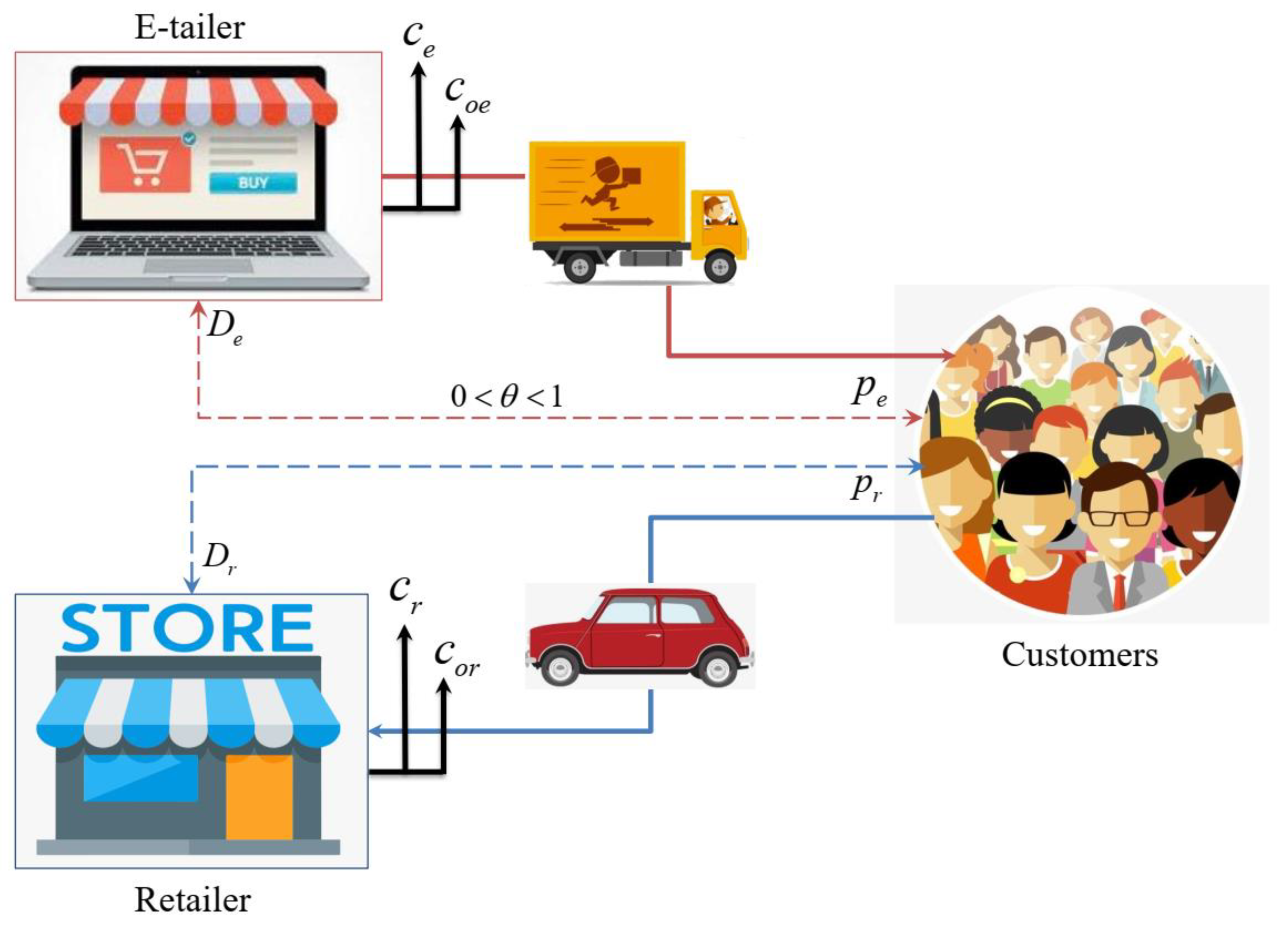
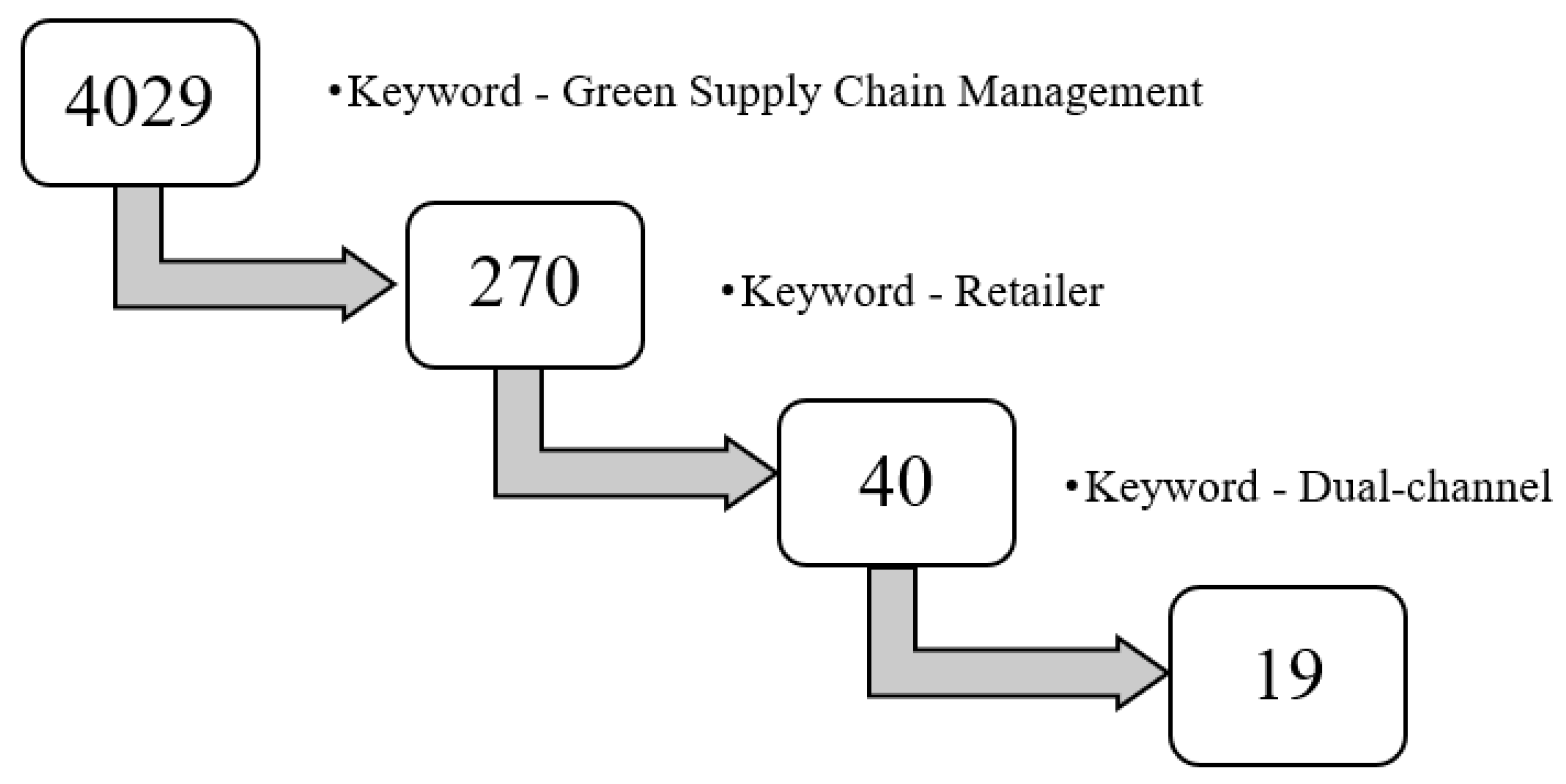
This section considered a market structure where both the r-store (brick and mortar retailer) and the e-store (online retailer) sell identical products to the customers. They are engaged in competition as they are targeting the same customer segment. The representational diagram of the model is shown in Figure 2.

Similar models can be found in [45,46,47]. For example, Amrouche and Yan (2016) [45] compared the benefit of wholesale pricing and quantity discount coordinating mechanisms under a dual-channel supply chain when the retailers are competing. In addition, Yan (2010) [46] considered a competing retailer and an online retailer to examine the benefit of demand forecast information sharing, and Yan and Pei (2015) [47] focused on the role of cooperative advertisements in a similar supply chain configuration.

In this study, the demand for the r-store and e-store is modeled as a function of price and emission reduction effort, as in Du et al. (2015) [48], who developed a low carbon-sensitive demand function for a single manufacturer. Furthermore, we adapted it to a dual-member scenario enabling us to study competition between two firms (r-store and e-store) as shown in Equations (1) and (2).

Demand for the r-store is:

$$D_r=a(1-\theta )-p_r{\left(\frac{c_{or}}{c_r}\right)}^{\alpha }+p_e{\left(\frac{c_{oe}}{c_e}\right)}^{\beta }$$

(1)

Demand for the e-store is:

$$D_e=a\theta -p_e{\left(\frac{c_{oe}}{c_e}\right)}^{\beta }+p_r{\left(\frac{c_{or}}{c_r}\right)}^{\alpha }$$

(2)

where a denotes basic market demand, i.e., the demand of a product when the price is zero ($D=a-bp$). The base demand varies from product to product. Not all products are demanded equally, even when it is free. The base demand declines linearly with an increase in price in the case of a linear demand function. In this study, the base demand ‘a’ is split between the r-store and e-store based on a parameter $\theta$ defined as the customer preference for the e-store. The greater value of $\theta$ implies greater demand for the e-store and vice versa. The value of θ varies according to product categories [49]. The value of base demand (a) is much higher than the other parameters of the model [50]. Further, p_r and p_e denote the price of the r-store and the e-store, respectively. Correspondingly, $c_r \mathrm{and} c_e$ denote carbon emission per unit product sold under the traditional mode of operation for the r-store and e-store.

After the r-store and e-store have engaged in green operations, carbon emissions decrease. We denote carbon emission per unit product sold under the green mode of operation as c_or and c_oe for r-store and e-store, respectively. Further, α and β correspondingly represent the demand sensitivity to the emission reduction effort of the r-store and e-store. The demand functions capture the dependence of demand on the price of the firm, the price of the competitor, the degree of emission reduction by the firm, and the degree of emission reduction by the competitor. The green operation reduced carbon emissions $c_{or}<c_r$ and c_oe < c_e, making the ratio $\frac{c_{oe}}{c_e}$ and $\frac{c_{or}}{c_r}$ less than 1. Further, it can be inferred that the term ${\left(\frac{c_{or}}{c_r}\right)}^{\alpha }$ is equivalent to the price-elasticity term in the linear demand function. The term ${\left(\frac{c_{or}}{c_r}\right)}^{\alpha }$ represents own-price sensitivity and cross-price sensitivity in the case of r-store’s demand and e-store’s demand, respectively. Similarly, the term ${\left(\frac{c_{oe}}{c_e}\right)}^{\beta }$ indicates cross-price sensitivity and own-price sensitivity for the r-store and e-store. The demand function captures the effect of carbon emission reduction through reduced price sensitivity. In other words, the consumers will prefer to buy from the r-store/e-store with lower carbon emissions, ceteris paribus. For ease of reporting and explanation, we define $\frac{c_{or}}{c_r}$ as η and $\frac{c_{oe}}{c_e}$ as μ making Equations (1) and (2) as follows:

Demand for the r-store is:

$$D_r^{}=a\left(1-\theta \right)-{\eta }^{\alpha }{p}_r^{}+{\mu }^{\beta }{p}_e^{}$$

(3)

Demand for the e-store is:

$$D_e^{}=a\theta -{\mu }^{\beta }{p}_e^{}+{\eta }^{\alpha }{p}_r^{}$$

(4)

The profit function of the r-store is:

$${\pi }_r^{}=\left(p_r^{}-{\eta }^{-\gamma }{m}_{or}\right)\left(a\left(1-\theta \right)-{\eta }^{\alpha }{p}_r^{}+{\mu }^{\beta }{p}_e^{}\right)$$

(5)

The profit function of the e-store is:

$${\pi }_e^{}=\left(p_e^{}-{\mu }^{-\delta }{m}_{er}\right)\left(a\theta -{\mu }^{\beta }{p}_e^{}+{\eta }^{\alpha }{p}_r^{}\right)$$

(6)

In the profit functions, ${\eta }^{-\gamma }{m}_{or}$ and ${\mu }^{-\delta }{m}_{er}$ represent the unit marginal cost for selling under the green operation mode for the r-store and e-store. γ and δ denote the elasticities of cost to emission reduction effort of the r-store and e-store. Likewise, $m_{or}$ and $m_{er}$ indicate the unit marginal cost for selling associated with the traditional mode of operation for the r-store and e-store. The rationale behind the mathematical form of the unit marginal cost for selling the green operation mode is that the higher the level of green operations, the higher the cost [48].

4. Equilibrium Analysis

In this section, game-theoretic models are developed for three-channel power configurations and are analyzed using equilibrium analysis. The channel power configurations considered are the (i) horizontal Nash (HN) configuration, (ii) R-store leader (RL) the Stackelberg configuration, and the (iii) E-store leader (EL) Stackelberg configuration. We derived and reported the optimal decisions for the channel members and the resulting profit corresponding to each channel configuration. The optimal decisions obtained under equilibrium analysis correspond to the Nash equilibrium. The Nash equilibrium of a noncooperative game is a profile of strategies, one for each player in the game, such that each player’s strategy maximizes his expected utility payoff against the given strategies of the other players [51]. In this study, the Nash equilibrium is the profile of pricing strategies of the r-store and e-store that maximize their respective profits.

4.1. HN Game-Equilibrium Analysis

Firstly, we report the equilibrium analysis of the HN game between the r-store and e-store. Here, since the channel power of the r-store and e-store is assumed to be comparable, a simultaneous game (Nash) has been employed. Both the r-store and e-store announce their price decision simultaneously. Based on the price, they realize the sales volume, respectively, to obtain profit. In this study, we have assumed that the r-store and e-store are able to satisfy the demand. In other words, we are not considering the lost sales and backlogs. Thus, the demand realization is termed sales volume.

Demand for the r-store and e-store are:

$$D_r^{NG}=a\left(1-\theta \right)-{\eta }^{\alpha }{p}_r^{NG}+{\mu }^{\beta }{p}_e^{NG}$$

(7)

$$D_e^{NG}=a\theta -{\mu }^{\beta }{p}_e^{NG}+{\eta }^{\alpha }{p}_r^{NG}$$

(8)

Profits of the r-store and e-store are:

$${\pi }_r^{NG}=\left(p_r^{NG}-{\eta }^{-\gamma }{m}_{or}\right)D_r^{NG}=\left(p_r^{NG}-{\eta }^{-\gamma }{m}_{or}\right)\left(a\left(1-\theta \right)-{\eta }^{\alpha }{p}_r^{NG}+{\mu }^{\beta }{p}_e^{NG}\right)$$

(9)

$${\pi }_e^{NG}=\left(p_e^{NG}-{\mu }^{-\delta }{m}_{er}\right)D_e^{NG}=\left(p_e^{NG}-{\mu }^{-\delta }{m}_{er}\right)\left(a\theta -{\mu }^{\beta }{p}_e^{NG}+{\eta }^{\alpha }{p}_r^{NG}\right)$$

(10)

Under the HN game, the r-store decides the optimal price given the price of the e-store.

$$p_r^{NG*}\in \underset{p_r^{NG}}{\arg \max }{\pi }_r^{NG}\left(p_r^{NG}/p_e^{NG}\right)$$

Similarly, the e-store decides on the optimal price given the price of the r-store.

$$p_e^{NG*}\in \underset{p_e^{NG}}{\arg \max }{\pi }_e^{NG}\left(p_e^{NG}/p_r^{NG}\right)$$

Both the channel members choose their optimal prices concurrently to obtain maximal profit. Since both ${\pi }_r^{NG}$ and ${\pi }_e^{NG}$ are concave in $p_r^{NG}$ and $p_e^{NG}$, respectively, (see Appendix A), the optimal values of $p_r^{NG}$ and $p_e^{NG}$ can be derived from the first-order condition (FOC) of ${\pi }_r^{NG}$ and ${\pi }_e^{NG}$, and are reported below.

Proposition 1.

The optimal price of the channel members under the HN game are:

$$p_r^{NG*}=\frac{1}{3}\left(\frac{a\left(2-\theta \right)}{{\eta }^{\alpha }}+\frac{m_{er}{\mu }^{\beta }}{{\eta }^{\alpha }{\mu }^{\delta }}+\frac{2m_{or}}{{\eta }^{\gamma }}\right)$$

(11)

$$p_e^{NG*}=\frac{1}{3{\eta }^{\gamma }{\mu }^{\beta +\delta }}\left(a{\eta }^{\gamma }{\mu }^{\delta }\left(1+\theta \right)+2{\eta }^{\gamma }{\mu }^{\beta }{m}_{er}+{\eta }^{\alpha }{\mu }^{\delta }{m}_{or}\right)$$

(12)

Substituting Equations (11) and (12) into the demand functions (i.e., Equations (7) and (8)) will provide the optimal sales volume of the channel members and are reported below.

Corollary 1.

The optimal sales volume of the channel members under the HN game are:

$$Q_r^{NG*}=\frac{1}{3}\left(a\left(2-\theta \right)+\frac{{\mu }^{\beta }{m}_{er}}{{\mu }^{\delta }}-\frac{{\eta }^{\alpha }{m}_{or}}{{\eta }^{\gamma }}\right)$$

(13)

$$Q_e^{NG*}=\frac{1}{3}\left(a\left(1+\theta \right)-\frac{m_{er}{\mu }^{\beta }}{{\mu }^{\delta }}+\frac{m_{or}{\eta }^{\alpha }}{{\eta }^{\gamma }}\right)$$

(14)

Substituting the values of $p_r^{NG*},p_e^{NG*},Q_r^{NG*} \mathrm{and} Q_e^{NG*}$ into the profit functions (i.e., Equations (9) and (10)) will provide the optimal profit for the channel members, as shown below.

Corollary 2.

The optimal profit for the channel members under the HN game are:

$${\pi }_r^{NG*}=\frac{1}{9{\eta }^{\alpha +2\gamma }{\mu }^{2\delta }}{\left({\eta }^{\gamma }{\mu }^{\beta }{m}_{er}-{\mu }^{\delta }\left({\eta }^{\alpha }{m}_{or}-a{\eta }^{\gamma }\left(2-\theta \right)\right)\right)}^2$$

(15)

$${\pi }_e^{NG*}=\frac{1}{9{\eta }^{2\gamma }{\mu }^{\beta +2\delta }}{\left({\eta }^{\gamma }{\mu }^{\beta }{m}_{er}-{\mu }^{\delta }\left(a{\eta }^{\gamma }\left(1+\theta \right)+{\eta }^{\alpha }{m}_{or}\right)\right)}^2$$

(16)

4.2. RL Stackelberg Game-Equilibrium Analysis

This section deals with the sequential game between the channel members under the channel leadership of the r-store. The order of decision-making is as follows:

(i) The r-store decides on the price and sales volume; (ii) the e-store notices the decisions of the r-store and then decides the optimal price and sales volume; (iii) the profit of the channel members is derived from the price and sales volume.

The sequential game is solved using backward induction. The sequence of the backward induction is as follows: (i) the optimal price of the e-store is obtained by optimizing the profit of the e-store; (ii) the r-store finds the optimal price by considering the price of the e-store; (iii) optimal sales volume of both the r-store and e-store are found out from the optimal prices; (iv) profits of the channel members are obtained from the optimal price and optimal sales volume. We present the backward induction as follows:

Demand for the r-store and e-store are:

$$D_r^{RL}=a\left(1-\theta \right)-{\eta }^{\alpha }{p}_r^{RL}+{\mu }^{\beta }{p}_e^{RL}$$

(17)

$$D_e^{RL}=a\theta -{\mu }^{\beta }{p}_e^{RL}+{\eta }^{\alpha }{p}_r^{RL}$$

(18)

The profit functions of the r-store and e-store are:

$${\pi }_r^{RL}=\left(p_r^{RL}-{\eta }^{-\gamma }{m}_{or}\right)D_r^{RL}=\left(p_r^{RL}-{\eta }^{-\gamma }{m}_{or}\right)\left(a\left(1-\theta \right)-{\eta }^{\alpha }{p}_r^{RL}+{\mu }^{\beta }{p}_e^{RL}\right)$$

(19)

$${\pi }_e^{RL}=\left(p_e^{RL}-{\mu }^{-\delta }{m}_{er}\right)D_e^{RL}=\left(p_e^{RL}-{\mu }^{-\delta }{m}_{er}\right)\left(a\theta -{\mu }^{\beta }{p}_e^{RL}+{\eta }^{\alpha }{p}_r^{RL}\right)$$

(20)

We first find the e-store’s optimal price as per the backward induction procedure. Then, the rational e-store finds an optimal price that maximizes its profit given the price of the r-store.

$$p_e^{RL*}\in \underset{p_e^{RL}}{\arg \max }{\pi }_e^{RL}\left(p_e^{RL}/p_r^{RL}\right)$$

Since ${\pi }_e^{RL}$ is concave with respect to $p_e^{RL}$ (See Appendix A), the optimal value of $p_e^{RL}$ is obtained from the FOC of the e-store’s profit as shown below.

The e-store’s optimal price, when the channel members are engaged in the Stackelberg game under the leadership of the r-store, is

$$p_e^{RL}=\frac{1}{2{\mu }^{\beta +\delta }}\left(a\theta {\mu }^{\delta }+m_{er}{\mu }^{\beta }+{\eta }^{\alpha }{\mu }^{\delta }{p}_r^{RL}\right)$$

(21)

As the leader, the r-store anticipates the best response from the e-store. Substitute $p_e^{RL}$ into ${\pi }_r^{RL}$ and obtain

$${\pi }_r^{RL}=\left(p_r^{RL}-{\eta }^{-\gamma }{m}_{or}\right)\left(a\left(1-\theta \right)-{\eta }^{\alpha }{p}_r^{RL}+\frac{1}{2{\mu }^{\delta }}\left(a\theta {\mu }^{\delta }+{\mu }^{\beta }{m}_{er}+{\eta }^{\alpha }{\mu }^{\delta }{p}_r^{RL}\right)\right)$$

(22)

Further, the r-store chooses its price to maximize the profit and is

$$p_r^{RL*}\in \underset{p_r^{RL}}{\arg \max }{\pi }_r^{RL}\left(p_r^{RL}/p_e^{RL}\right)$$

Since ${\pi }_r^{RL}$ is concave with respect to $p_r^{RL}$ (See Appendix A), the optimal value of $p_r^{RL}$ is obtained from the FOC of ${\pi }_r^{RL}$. Further, substituting $p_r^{RL*}$ into Equation (21) will provide the r-store’s optimal price. We present the optimal prices below.

Proposition 2.

The optimal prices of the channel members under the RL game are:

$$p_r^{RL*}=\frac{1}{2{\eta }^{\alpha +\gamma }{\mu }^{\delta }}\left(a{\eta }^{\gamma }{\mu }^{\delta }\left(2-\theta \right)+{\eta }^{\gamma }{\mu }^{\beta }{m}_{er}+{\eta }^{\alpha }{\mu }^{\delta }{m}_{or}\right)$$

(23)

$$p_e^{RL*}=\frac{1}{4}\left(\frac{3m_{er}}{{\mu }^{\delta }}+\frac{\left(a{\eta }^{\gamma }\left(2+\theta \right)+{\eta }^{\alpha }{m}_{or}\right)}{{\eta }^{\gamma }{\mu }^{\beta }}\right)$$

(24)

Further, substituting Equations (23) and (24) into Equations (17) and (18) will provide the optimal sales volume of channel members, as reported in the following corollary.

Corollary 3.

The optimal sales volume of the channel members under the RL game are:

$$Q_r^{RL*}=\frac{1}{4}\left(a\left(2-\theta \right)+\frac{{\mu }^{\beta }}{{\mu }^{\delta }}{m}_{er}-\frac{{\eta }^{\alpha }}{{\eta }^{\gamma }}{m}_{or}\right)$$

(25)

$$Q_e^{RL*}=\frac{1}{4}\left(a\left(2+\theta \right)-\frac{{\mu }^{\beta }}{{\mu }^{\delta }}{m}_{er}+\frac{{\eta }^{\alpha }}{{\eta }^{\gamma }}{m}_{or}\right)$$

(26)

Substituting the optimal decisions of the r-store and e-store into Equations (19) and (20) will provide the optimal profit for the channel members, as reported below.

Corollary 4.

The optimal profit for the channel members under the RL game are:

$${\pi }_r^{RL*}=\frac{1}{8{\eta }^{\alpha +2\gamma }{\mu }^{2\delta }}{\left({\eta }^{\gamma }{\mu }^{\beta }{m}_{er}-{\mu }^{\delta }\left({\eta }^{\alpha }{m}_{or}-a{\eta }^{\gamma }\left(2-\theta \right)\right)\right)}^2$$

(27)

$${\pi }_e^{RL*}=\frac{1}{16{\eta }^{2\gamma }{\mu }^{\beta +2\delta }}{\left({\eta }^{\gamma }{\mu }^{\beta }{m}_{er}-{\mu }^{\delta }\left(a{\eta }^{\gamma }\left(2+\theta \right)+{\eta }^{\alpha }{m}_{or}\right)\right)}^2$$

(28)

4.3. EL Stackelberg Game-Equilibrium Analysis

The equilibrium analysis presented in this section is the complementary case of the equilibrium analysis presented in the previous section with a role reversal between the r-store and e-store. The e-store, as the leader, decides the price and sales volume first to maximize its profit. The r-store, as the follower, observes the e-store’s decisions and makes its own decisions to maximize its profit. As in model 2, we apply backward induction to solve the Stackelberg game as follows.

Demand for the r-store and e-store are:

$$D_r^{EL}=a\left(1-\theta \right)-{\eta }^{\alpha }{p}_r^{EL}+{\mu }^{\beta }{p}_e^{EL}$$

(29)

$$D_e^{EL}=a\theta -{\mu }^{\beta }{p}_e^{EL}+{\eta }^{\alpha }{p}_r^{EL}$$

(30)

Profit of the r-store and e-store are:

$${\pi }_r^{EL}=\left(p_r^{EL}-{\eta }^{-\gamma }{m}_{or}\right)D_r^{EL}=\left(p_r^{EL}-{\eta }^{-\gamma }{m}_{or}\right)\left(a\left(1-\theta \right)-{\eta }^{\alpha }{p}_r^{EL}+{\mu }^{\beta }{p}_e^{EL}\right)$$

(31)

$${\pi }_e^{EL}=\left(p_e^{EL}-{\mu }^{-\delta }{m}_{er}\right)D_e^{EL}=\left(p_e^{EL}-{\mu }^{-\delta }{m}_{er}\right)\left(a\theta -{\mu }^{\beta }{p}_e^{EL}+{\eta }^{\alpha }{p}_r^{EL}\right)$$

(32)

We first find the r-store’s optimal price per the backward induction procedure. The rational r-store finds an optimal price to maximize its profit given the price of the e-store, i.e.,

$$p_r^{EL*}\in \underset{p_r^{EL}}{\arg \max }{\pi }_r^{EL}\left(p_r^{EL}/p_e^{EL}\right)$$

Since ${\pi }_r^{RL}$ is concave with respect to $p_r^{RL}$ (see Appendix A), the optimal value of $p_r^{RL}$ is obtained from the FOC of the e-store’s profit.

The r-store’s optimal price is

$$p_r^{EL}=\frac{1}{2{\eta }^{\alpha +\gamma }}\left(a{\eta }^{\gamma }\left(1-\theta \right)+{\eta }^{\alpha }{m}_{or}+{\eta }^{\gamma }{\mu }^{\beta }{p}_e^{EL}\right)$$

(33)

The e-store, as the leader, anticipates the best response from the r-store. Mathematically, we substitute $p_r^{EL}$ into ${\pi }_e^{EL}$ and obtain

$${\pi }_e^{EL}=\left(p_e^{EL}-{\mu }^{-\delta }{m}_{er}\right)\left(a\theta -{\mu }^{\beta }{p}_e^{EL}+\frac{1}{2}{\eta }^{-\gamma }\left(a{\eta }^{\gamma }\left(1-\theta \right)+{\eta }^{\alpha }{m}_{or}+{\eta }^{\gamma }{\mu }^{\beta }{p}_e^{EL}\right)\right)$$

(34)

Further, the e-store deciding its price to maximize the profit is

$$p_e^{EL*}\in \underset{p_e^{EL}}{\arg \max }{\pi }_e^{EL}\left(p_e^{EL}/p_r^{EL}\right)$$

Since ${\pi }_e^{EL}$ is concave with respect to $p_e^{EL}$ (see Appendix A), the optimal value of $p_e^{EL}$ is obtained from the FOC of ${\pi }_e^{EL}$ and is reported below.

Proposition 3.

The optimal price of the channel members under the EL game, are:

$$p_r^{EL*}=\frac{1}{4}\left(\frac{a\left(3-\theta \right)}{{\eta }^{\alpha }}+\frac{m_{er}{\mu }^{\beta }}{{\eta }^{\alpha }{\mu }^{\delta }}+\frac{3m_{or}}{{\eta }^{\gamma }}\right)$$

(35)

$$p_e^{EL*}=\frac{1}{2{\eta }^{\gamma }{\mu }^{\beta +\delta }}\left(a{\eta }^{\gamma }{\mu }^{\delta }\left(1+\theta \right)+{\eta }^{\gamma }{\mu }^{\beta }{m}_{er}+{\eta }^{\alpha }{\mu }^{\delta }{m}_{or}\right)$$

(36)

Further, substituting Equations (35) and (36) into Equations (29) and (30) will provide the optimal sales volume of channel members, as reported below.

Corollary 3.

The optimal sales volume for the channel members under the EL game are:

$$Q_r^{EL*}=\frac{1}{4}\left(a\left(3-\theta \right)+\frac{{\mu }^{\beta }}{{\mu }^{\delta }}{m}_{er}-\frac{{\eta }^{\alpha }}{{\eta }^{\gamma }}{m}_{or}\right)$$

(37)

$$Q_e^{EL*}=\frac{1}{4}\left(a\left(1+\theta \right)-\frac{{\mu }^{\beta }}{{\mu }^{\delta }}{m}_{er}+\frac{{\eta }^{\alpha }}{{\eta }^{\gamma }}{m}_{or}\right)$$

(38)

Substituting the optimal decisions of channel members into Equations (31) and (32) will provide the channel members’ optimal profit as reported below.

Corollary 4.

The optimal profit for the channel members under the EL game are:

$${\pi }_r^{EL*}=\frac{1}{16{\eta }^{\alpha +2\gamma }{\mu }^{2\delta }}{\left({\eta }^{\gamma }{\mu }^{\beta }{m}_{er}-{\mu }^{\delta }\left({\eta }^{\alpha }{m}_{or}-a{\eta }^{\gamma }\left(3-\theta \right)\right)\right)}^2$$

(39)

$${\pi }_e^{EL*}=\frac{1}{8{\eta }^{2\gamma }{\mu }^{\beta +2\delta }}{\left({\eta }^{\gamma }{\mu }^{\beta }{m}_{er}-{\mu }^{\delta }\left(a{\eta }^{\gamma }\left(1+\theta \right)+{\eta }^{\alpha }{m}_{or}\right)\right)}^2$$

(40)

4.4. Comparison among Channel Power Structures

This section deals with comparing the optimal decisions of the channel members among different channel power structures. First, we compare the prices of the r-store across the HN, RL, and EL games to arrive at the following propositions.

Proposition 4a.

The r-store’s optimal price under the HN game is dominated by the r-store’s optimal price under the RL game when the base demand $a>\frac{\left({\eta }^{\alpha }{\mu }^{\delta }{m}_{or}-{\eta }^{\gamma }{\mu }^{\beta }{m}_{er}\right)}{{\eta }^{\gamma }{\mu }^{\delta }(2-\theta )}$

Proposition 4b.

The r-store’s optimal price under the HN game is dominated by the r-store’s optimal price under the EL game when the base demands$a>\frac{\left({\eta }^{\gamma }{\mu }^{\beta }{m}_{er}-{\eta }^{\alpha }{\mu }^{\delta }{m}_{or}\right)}{{\eta }^{\gamma }{\mu }^{\delta }(1+\theta )}$

Proposition 4c.

The r-store’s optimal price under the RL game dominates the r-store’s optimal price under the EL game when the base demand $a>\frac{\left({\eta }^{\alpha }{\mu }^{\delta }{m}_{or}-{\eta }^{\gamma }{\mu }^{\beta }{m}_{er}\right)}{{\eta }^{\gamma }{\mu }^{\delta }(1-\theta )}$

Next, compare the r-store’s optimal sales volume among the three-channel power structures through the following propositions.

Proposition 5a.

The r-store’s optimal sales volume under the HN game dominates the r-store’s optimal sales volume under the RL game when the base demand $a>\frac{\left({\eta }^{\alpha }{\mu }^{\delta }{m}_{or}-{\eta }^{\gamma }{\mu }^{\beta }{m}_{er}\right)}{(2-\theta ){\eta }^{\gamma }{\mu }^{\delta }}$

Proposition 5b.

The r-store’s optimal sales volume under the HN game is dominated by the r-store’s optimal sales volume under the EL game when the base demand $a>\frac{\left({\eta }^{\gamma }{\mu }^{\beta }{m}_{er}-{\eta }^{\alpha }{\mu }^{\delta }{m}_{or}\right)}{(1+\theta ){\eta }^{\gamma }{\mu }^{\delta }}$

Proposition 5c.

The r-store’s optimal sales volume under the RL game is dominated by the r-store’s optimal sales volume under the EL game, irrespective of the value of base demand.

We compare the e-store’s optimal price among the HN, RL, and EL games, and the results are shown in the following proposition.

Proposition 6a.

The e-store’s optimal price under the HN game is dominated by the e-store’s optimal price under the RL game $a>\frac{\left({\eta }^{\alpha }{\mu }^{\delta }{m}_{or}-{\eta }^{\gamma }{\mu }^{\beta }{m}_{er}\right)}{{\eta }^{\gamma }{\mu }^{\delta }(2-\theta )}$

Proposition 6b.

The e-store’s optimal price under the HN game is dominated by the e-store’s optimal price under the EL game when the base demand $a>\frac{\left({\eta }^{\gamma }{\mu }^{\beta }{m}_{er}-{\eta }^{\alpha }{\mu }^{\delta }{m}_{or}\right)}{{\eta }^{\gamma }{\mu }^{\delta }\theta }$

Proposition 6c.

The e-store’s optimal price under the RL game is dominated by the e-store’s optimal price under the EL game when the base demand, $a>\frac{\left({\eta }^{\gamma }{\mu }^{\beta }{m}_{er}-{\eta }^{\alpha }{\mu }^{\delta }{m}_{or}\right)}{\theta {\eta }^{\gamma }{\mu }^{\delta }}$

To find the impact of price on the sales volume, we compare the e-store’s optimal sales volume among the HN, RL, and EL games and present the results in the following propositions.

Proposition 7a.

The e-store’s optimal sales volume under the HN game is dominated by the e-store’s optimal sales volume under the RL game when the base demand $a>\frac{\left({\eta }^{\alpha }{\mu }^{\delta }{m}_{or}-{\eta }^{\gamma }{\mu }^{\beta }{m}_{er}\right)}{{\eta }^{\gamma }{\mu }^{\delta }(2-\theta )}$

Proposition 7b.

The e-store’s optimal sales volume under the HN game dominates the e-store’s optimal sales volume under the EL game when $a>\frac{\left({\eta }^{\gamma }{\mu }^{\beta }{m}_{er}-{\eta }^{\alpha }{\mu }^{\delta }{m}_{or}\right)}{{\eta }^{\gamma }{\mu }^{\delta }(1+\theta )}$

Proposition 7c.

The e-store’s optimal sales volume under the RL game dominates the e-store’s optimal sales volume under the EL game irrespective of the value of base demand.

Now, we compare the profit of the r-store among the HN, RL, and EL games and arrive at the following propositions.

Proposition 8a.

The r-store’s optimal profit under the HN game is dominated by the r-store’s optimal profit under the RL game, irrespective of the product’s base demand and online channel preference.

Proposition 8b.

The r-store’s optimal profit under the HN game is dominated by the r-store’s optimal profit under the EL game when the base demand,

$$\begin{array}{l}a>Max\left\{a_1,a_2\right\}\\ \mathrm{where}\\ a_1=\frac{\left({\eta }^{\gamma }{\mu }^{\beta }{m}_{er}-{\eta }^{\alpha }{\mu }^{\delta }{m}_{or}\right)}{{\eta }^{\gamma }{\mu }^{\delta }(1+\theta )}\\ a_2=\frac{7\left({\eta }^{\gamma }{\mu }^{\beta }{m}_{er}-{\eta }^{\alpha }{\mu }^{\delta }{m}_{or}\right)}{{\eta }^{\gamma }{\mu }^{\delta }(7\theta -17)}\end{array}$$

Proposition 8c.

The r-store’s optimal profit under the RL game is dominated by the r-store’s optimal profit under the EL game when the base demand,

$$a>Max\left\{a_3,a_4\right\}$$

$$\begin{array}{l}\mathrm{where} \\ a_3=\frac{{\eta }^{\alpha +\gamma }{\mu }^{2\delta }{m}_{or}(1-\theta )-{\eta }^{2\gamma }{\mu }^{\beta +\delta }{m}_{er}(1-\theta )-\sqrt{2}\sqrt{{\eta }^{4\gamma }{\mu }^{2\beta +2\delta }{m}_{er}^2-2{\eta }^{\alpha +3\gamma }{\mu }^{\beta +3\delta }{m}_{er}{m}_{or}+{\eta }^{2\alpha +2\gamma }{\mu }^{4\delta }{m}_{or}^2}}{{\eta }^{2\gamma }{\mu }^{2\delta }({\theta }^2-2\theta -1)}\\ a_4=\frac{{\eta }^{\alpha +\gamma }{\mu }^{2\delta }{m}_{or}(1-\theta )-{\eta }^{2\gamma }{\mu }^{\beta +\delta }{m}_{er}(1-\theta )+\sqrt{2}\sqrt{{\eta }^{4\gamma }{\mu }^{2\beta +2\delta }{m}_{er}^2-2{\eta }^{\alpha +3\gamma }{\mu }^{\beta +3\delta }{m}_{er}{m}_{or}+{\eta }^{2\alpha +2\gamma }{\mu }^{4\delta }{m}_{or}^2}}{{\eta }^{2\gamma }{\mu }^{2\delta }({\theta }^2-2\theta -1)}\end{array}$$

Now, we compare the profit of the e-store among the HN, RL, and EL games and obtain the following propositions below.

Proposition 9a.

The e-store’s optimal profit under the HN game is dominated by the e-store’s optimal profit under the RL game when the base demand,

$$\begin{array}{l}a>Max\left\{a_5,a_6\right\}\\ \mathrm{where}\\ a_5=\frac{\left({\eta }^{\alpha }{\mu }^{\delta }{m}_{or}-{\eta }^{\gamma }{\mu }^{\beta }{m}_{er}\right)}{{\eta }^{\gamma }{\mu }^{\delta }(2-\theta )}\\ a_6=\frac{7\left({\eta }^{\gamma }{\mu }^{\beta }{m}_{er}-{\eta }^{\alpha }{\mu }^{\delta }{m}_{or}\right)}{{\eta }^{\gamma }{\mu }^{\delta }(10\theta +7)}\end{array}$$

Proposition 9b.

The e-store’s optimal profit under the HN game is dominated by the e-store’s optimal profit under the EL game, irrespective of the value of base demand.

Proposition 9c.

The e-store’s optimal profit under the EL game is dominated by the e-store’s optimal profit under the RL game when the base demand,

$$\begin{array}{l}a>Max\left\{a_7,a_8\right\}\\ a_7=\frac{{\eta }^{2\gamma }\theta {\mu }^{\beta +\delta }{m}_{er}-{\eta }^{\alpha +\gamma }\theta {\mu }^{2\delta }{m}_{or}-\sqrt{2}\sqrt{{\eta }^{4\gamma }{\mu }^{2\beta +2\delta }{m}_{er}^2-2{\eta }^{\alpha +3\gamma }{\mu }^{\beta +3\delta }{m}_{er}{m}_{or}+{\eta }^{2\alpha +2\gamma }{\mu }^{4\delta }{m}_{or}^2}}{{\eta }^{2\gamma }{\mu }^{2\delta }({\theta }^2-2)}\\ a_8=\frac{{\eta }^{2\gamma }\theta {\mu }^{\beta +\delta }{m}_{er}-{\eta }^{\alpha +\gamma }\theta {\mu }^{2\delta }{m}_{or}+\sqrt{2}\sqrt{{\eta }^{4\gamma }{\mu }^{2\beta +2\delta }{m}_{er}^2-2{\eta }^{\alpha +3\gamma }{\mu }^{\beta +3\delta }{m}_{er}{m}_{or}+{\eta }^{2\alpha +2\gamma }{\mu }^{4\delta }{m}_{or}^2}}{{\eta }^{2\gamma }{\mu }^{2\delta }({\theta }^2-2)}\end{array}$$

5. Numerical Validation of Propositions

This section reports the numerical validation of the propositions derived in the previous section. The rationale for numerical examples is the intractability of mathematical expressions derived from the equilibrium analysis. Moreover, it is implausible to obtain managerial insights from complex mathematical expressions. Therefore, we resort to a numerical example and cover three cases for the generalizability of the results.

(i)

Case 1: The numerical values of parameters of the r-store and e-store are identical.

(ii)

Case 2: The numerical values of parameters of the r-store are greater than that of the e-store.

(iii)

Case 3: The numerical values of parameters of the r-store are lower than that of the e-store.

We have considered three subcases under each case based on the value of base demand.

(i)

Sub-case 1: Low base demand (a = 50).

(ii)

Sub-case 2: Moderate base demand (a = 100).

(iii)

Sub-case 3: High base demand (a = 150).

The numerical values of other parameters are mostly selected from previous studies in the extant literature [48]. The logical relationships among the parameters have also been considered while selecting the numerical values. For instance, the value of a is much larger than the other parameters of the model.

Case 1.

The numerical values of the parameters of the r-store and e-store are equal.

The selected parametric values considered for Case 1 are

$$\theta =0.5,\alpha =\beta =1.2,\gamma =\delta =2,m_{or}=m_{er}=10,\eta =\mu =0.5$$

The numerical results of the HN, RL, and EL games are presented in

Table 1. Optimal decisions of channel members under the HN game—Case 1.

	${\mathit{p}}_{\mathit{r}}^{\mathit{H}{\mathit{N}}^{*}}$	${\mathit{p}}_{\mathit{e}}^{\mathit{H}{\mathit{N}}^{*}}$	${\mathit{Q}}_{\mathit{r}}^{\mathit{H}{\mathit{N}}^{*}}$	${\mathit{Q}}_{\mathit{e}}^{\mathit{H}{\mathit{N}}^{*}}$	${\mathit{\pi }}_{\mathit{r}}^{\mathit{H}{\mathit{N}}^{*}}$	${\mathit{\pi }}_{\mathit{e}}^{\mathit{H}{\mathit{N}}^{*}}$	${\mathit{\pi }}_{\mathit{S}\mathit{C}}^{\mathit{H}{\mathit{N}}^{*}}$
a = 50	97.43	97.43	25	25	1435.87	1435.87	2871.74
a = 100	154.87	154.87	50	50	5743.49	5743.49	11,482.8
a = 150	212.3	212.3	75	75	12,922.9	12,922.9	25,845.8

,

Table 2. Optimal decisions of channel members under the RL game—Case 1.

	${\mathit{p}}_{\mathit{r}}^{\mathit{R}{\mathit{L}}^{*}}$	${\mathit{p}}_{\mathit{e}}^{\mathit{R}{\mathit{L}}^{*}}$	${\mathit{Q}}_{\mathit{r}}^{\mathit{R}{\mathit{L}}^{*}}$	${\mathit{Q}}_{\mathit{e}}^{\mathit{R}{\mathit{L}}^{*}}$	${\mathit{\pi }}_{\mathit{r}}^{\mathit{R}{\mathit{L}}^{*}}$	${\mathit{\pi }}_{\mathit{e}}^{\mathit{R}{\mathit{L}}^{*}}$	${\mathit{\pi }}_{\mathit{S}\mathit{C}}^{\mathit{R}{\mathit{L}}^{*}}$
a = 50	126.15	111.79	18.75	31.25	1615.36	2243.55	3858.91
a = 100	212.3	183.58	37.5	62.5	6461.43	8974.21	15,435.6
a = 150	298.45	255.38	56.25	93.75	14,538.2	20,192	34,730.2

and

Table 3. Optimal decisions of channel members under the EL game—Case 1.

	${\mathit{p}}_{\mathit{r}}^{\mathit{E}{\mathit{L}}^{*}}$	${\mathit{p}}_{\mathit{e}}^{\mathit{E}{\mathit{L}}^{*}}$	${\mathit{Q}}_{\mathit{r}}^{\mathit{E}{\mathit{L}}^{*}}$	${\mathit{Q}}_{\mathit{e}}^{\mathit{E}{\mathit{L}}^{*}}$	${\mathit{\pi }}_{\mathit{r}}^{\mathit{E}{\mathit{L}}^{*}}$	${\mathit{\pi }}_{\mathit{e}}^{\mathit{E}{\mathit{L}}^{*}}$	${\mathit{\pi }}_{\mathit{S}\mathit{C}}^{\mathit{E}{\mathit{L}}^{*}}$
a = 50	111.79	126.15	31.25	18.75	2243.55	1615.36	3858.91
a = 100	183.58	212.3	62.5	37.5	8974.21	6461.43	15,435.6
a = 150	255.38	298.45	93.75	56.25	20,192	14,538.2	34,730.2

, respectively, for the three cases under consideration.

Optimal price of r-store: From Table 1 and Table 2, it can be observed that the r-store’s optimal price under the HN game is lower than that under the RL game. Thus, the numerical example is in line with Proposition 4a. The threshold value of base demand established under Proposition 4a, i.e., $\frac{\left({\eta }^{\alpha }{\mu }^{\delta }{m}_{or}-{\eta }^{\gamma }{\mu }^{\beta }{m}_{er}\right)}{{\eta }^{\gamma }{\mu }^{\delta }(2-\theta )}$, is found to be 34.81, which is less than the lowest base demand under consideration, i.e., 50, leading to the numerical validation of Proposition 4a. Similarly, Table 1 and Table 3 show that the r-store’s optimal price under the HN game is lower than that under the EL game, as established in Proposition 4b. It can be noted that the numerical value of the threshold of base demand as established in Proposition 4b, i.e., $\frac{\left({\eta }^{\gamma }{\mu }^{\beta }{m}_{er}-{\eta }^{\alpha }{\mu }^{\delta }{m}_{or}\right)}{{\eta }^{\gamma }{\mu }^{\delta }(1+\theta )}$, is −34.81, making the feasible threshold value 0 since demand cannot be negative. Since the lowest base demand under consideration, i.e., 50, is greater than the threshold value, Proposition 4b is numerically validated. Now, by comparing the r-store’s optimal price between Table 2 and Table 3, it can be found that the r-store’s optimal price under the RL game is higher than that under the EL game. Therefore, the numerical value of the threshold value of base demand, i.e., $\frac{\left({\eta }^{\alpha }{\mu }^{\delta }{m}_{or}-{\eta }^{\gamma }{\mu }^{\beta }{m}_{er}\right)}{{\eta }^{\gamma }{\mu }^{\delta }(1-\theta )}$ is 0, leading to the verification of Proposition 4c.

Optimal sales volume of r-store: Now, comparing the r-store’s optimal sales volume from Table 1 and Table 2, it can be observed that the optimal sales volume under the HN game is higher than that under the RL game, as established in Proposition 5a. The threshold value of base demand in Proposition 5a for this condition is numerically zero. Since all the base demand values considered for the numerical example are greater than zero, it can be stated that Proposition 5a is numerically validated. Next, the r-store’s optimal sales volume is compared between the HN and EL games, and it can be seen from Table 1 and Table 3 that the optimal r-store’s optimal sales volume is lower under the HN game than in the EL game. This observation is consistent with Proposition 5b. The threshold value of base demand in Proposition 5b under the numerical example is 0, as in the case of Proposition 4c and Proposition 5a. Comparing the r-store’s optimal sales volume between the RL and EL games observes that the optimal sales volume is lower under the RL game than in the EL game, as established in Proposition 5c.

Optimal price of e-store: Now, compare the e-store’s optimal price among different channel power structures. Table 1 and Table 2 show that the e-store’s optimal price under the HN game is lower than that under the RL game, as established in Proposition 6a. The threshold value of base demand in Proposition 6a is $\frac{\left({\eta }^{\alpha }{\mu }^{\delta }{m}_{or}-{\eta }^{\gamma }{\mu }^{\beta }{m}_{er}\right)}{{\eta }^{\gamma }{\mu }^{\delta }(2-\theta )}$, and the corresponding numerical value is 34.81. Since the lowest base demand used in the numerical example is 50, which is higher than 34.81, the condition $a>\frac{\left({\eta }^{\alpha }{\mu }^{\delta }{m}_{or}-{\eta }^{\gamma }{\mu }^{\beta }{m}_{er}\right)}{{\eta }^{\gamma }{\mu }^{\delta }(2-\theta )}$ is satisfied. While comparing the e-store’s optimal price between the HN game and EL game, the e-store’s optimal price under the HN game is lower than that under the EL game, as already established under Proposition 6b. Therefore, the condition under Proposition 6b is $a>\frac{\left({\eta }^{\gamma }{\mu }^{\beta }{m}_{er}-{\eta }^{\alpha }{\mu }^{\delta }{m}_{or}\right)}{{\eta }^{\gamma }{\mu }^{\delta }\theta }$. The RHS of this inequality can be numerically assessed, and the value is -34.81. For practical consideration, the threshold value has to be taken as 0. Since the lowest base demand employed for the numerical example is 50, we can infer that Proposition 6b is numerically verified. Now, comparing the e-store’s optimal price between RL and EL games, we can state that the e-store’s optimal price under the EL game is higher than that under the HN game. This observation is in line with Proposition 6c, and the condition for Proposition 6c to be satisfied is $a>\frac{\left({\eta }^{\gamma }{\mu }^{\beta }{m}_{er}-{\eta }^{\alpha }{\mu }^{\delta }{m}_{or}\right)}{\theta {\eta }^{\gamma }{\mu }^{\delta }}$. This condition is the same as Proposition 6b, and the numerical value obtained corresponding to the RHS of the inequality is −34.81, which is greater than 50; therefore, the condition is satisfied.

Optimal sales volume of the e-store: The comparison of sales volume of the e-store among the channel power structures yields the following observations. By examining Table 1, Table 2 and Table 3, it can be seen that the e-store’s optimal sales volume is highest under the RL game, followed by the HN game, and lowest under the EL game. The numerical values corresponding to the e-store’s optimal sales volume align with Propositions 7a, 7b, and 7c. The condition for the fulfillment of Proposition 7a is $a>\frac{\left({\eta }^{\alpha }{\mu }^{\delta }{m}_{or}-{\eta }^{\gamma }{\mu }^{\beta }{m}_{er}\right)}{{\eta }^{\gamma }{\mu }^{\delta }(2-\theta )}$. The numerical value of the RHS of the inequality is 34.81, which is smaller than 50, hence the numerical validation of Proposition 7a. The condition for the fulfillment of Proposition 7b is $a>\frac{\left({\eta }^{\gamma }{\mu }^{\beta }{m}_{er}-{\eta }^{\alpha }{\mu }^{\delta }{m}_{or}\right)}{{\eta }^{\gamma }{\mu }^{\delta }(1+\theta )}$. The numerical value of the RHS of the inequality is -34.81 (i.e., 0), which is smaller than 50, hence the numerical validation of Proposition 7b. Table 2 and Table 3 show that the e-store’s optimal sales volume under the RL game is higher than that under the EL game, which is in line with Proposition 7c.

Optimal profit of the r-store: Now, we examine the r-store’s profit among the channel power structures, and it can be observed that the r-store’s profit is highest under the EL game, followed by the RL game, and lowest under the HN game. This result agrees with Propositions 8a, 8b, and 8c. The condition for the fulfillment of Proposition 8a is unrelated to the value of base demand, and the condition for the fulfillment of Proposition 8b is the threshold value of base demand $a>Max\left\{a_1,a_2\right\}$. We examined the numerical value of the base demand threshold values and found that both the threshold values are zeroes for the given set of numerical values, and hence Proposition 8b is numerically validated. Now, we examine the threshold value of the base demand corresponding to Proposition 8c. The numerical value corresponding to $a_3$ is $2.72\times {10}^{-7}\approx 0$ and a₄ is $-2.72\times {10}^{-7}\approx 0$. Since the lowest base demand employed for numerical example is 50, greater than the threshold value, the condition $a>Max\left\{a_3,a_4\right\}$ is fulfilled, and Proposition 8c is numerically verified.

Optimal profit of the e-store: Now, we examine the e-store’s profit among the channel power structures. Table 1, Table 2 and Table 3 show that the profit of the e-store is highest under the RL game, followed by the EL game, and lowest under the HN game. This observation is consistent with Proposition 9a, 9b, and 9c, subjected to the fulfillment of base demand conditions. The base demand condition corresponding to Proposition 9a to be fulfilled is as follows:$a>Max\left\{a_5,a_6\right\}$. The numerical value of the threshold base demand is zero, and hence Proposition 9a is numerically valid. In the case of Proposition 9b, there is no condition to be fulfilled with respect to the base demand. The condition in the case of Proposition 9c is $a>Max\left\{a_7,a_8\right\}$. We find the numerical values of $a_7$ and a₈ as is $2.72\times {10}^{-7}$ and $-2.72\times {10}^{-7}$, respectively. Since the maximum of $a_7$ and a₈ is less than the lowest base demand under consideration, i.e., 50, it can be stated that the condition for Proposition 9c has been fulfilled.

Case 2.

The numerical values of parameters of the r-store are higher than that of the e-store.

The selected parametric values considered for Case 2 are

$$\theta =0.5,\alpha =2,\beta =1.2,\gamma =3,\delta =2,m_{or}=20,m_{er}=10,\eta =0.8,\mu =0.5$$

We have checked the consistency of the propositions with respect to the numerical example as we did in Case 1 and found that all propositions are valid under Case 2, i.e., when the numerical values of parameters of the r-store are higher than that of the e-store [

Table 4. Optimal decisions of channel members under the HN game—Case 2.

	${\mathit{p}}_{\mathit{r}}^{\mathit{H}{\mathit{N}}^{*}}$	${\mathit{p}}_{\mathit{e}}^{\mathit{H}{\mathit{N}}^{*}}$	${\mathit{Q}}_{\mathit{r}}^{\mathit{H}{\mathit{N}}^{*}}$	${\mathit{Q}}_{\mathit{e}}^{\mathit{H}{\mathit{N}}^{*}}$	${\mathit{\pi }}_{\mathit{r}}^{\mathit{H}{\mathit{N}}^{*}}$	${\mathit{\pi }}_{\mathit{e}}^{\mathit{H}{\mathit{N}}^{*}}$	${\mathit{\pi }}_{\mathit{S}\mathit{C}}^{\mathit{H}{\mathit{N}}^{*}}$
a = 50	74.17	103.24	22.47	27.52	788.93	1741.15	2530.08
a =100	113.23	160.68	47.47	52.52	3520.98	6339.35	9860.34
a = 150	152.29	218.11	72.47	77.52	8206.17	13,809.3	22,015.47

,

Table 5. Optimal decisions of channel members under the RL game—Case 2.

	${\mathit{p}}_{\mathit{r}}^{\mathit{R}{\mathit{L}}^{*}}$	${\mathit{p}}_{\mathit{e}}^{\mathit{R}{\mathit{L}}^{*}}$	${\mathit{Q}}_{\mathit{r}}^{\mathit{R}{\mathit{L}}^{*}}$	${\mathit{Q}}_{\mathit{e}}^{\mathit{R}{\mathit{L}}^{*}}$	${\mathit{\pi }}_{\mathit{r}}^{\mathit{R}{\mathit{L}}^{*}}$	${\mathit{\pi }}_{\mathit{e}}^{\mathit{R}{\mathit{L}}^{*}}$	${\mathit{\pi }}_{\mathit{S}\mathit{C}}^{\mathit{R}{\mathit{L}}^{*}}$
a = 50	91.72	116.15	16.85	33.14	887.54	2524.24	3411.78
a =100	150.32	187.94	35.6	64.39	3961.11	9527.31	13,488.42
a = 150	208.91	259.73	54.35	95.64	9231.94	21,017.49	30,249.43

and

Table 6. Optimal decisions of channel members under EL game—Case 2.

	${\mathit{p}}_{\mathit{r}}^{\mathit{E}{\mathit{L}}^{*}}$	${\mathit{p}}_{\mathit{e}}^{\mathit{E}{\mathit{L}}^{*}}$	${\mathit{Q}}_{\mathit{r}}^{\mathit{E}{\mathit{L}}^{*}}$	${\mathit{Q}}_{\mathit{e}}^{\mathit{E}{\mathit{L}}^{*}}$	${\mathit{\pi }}_{\mathit{r}}^{\mathit{E}{\mathit{L}}^{*}}$	${\mathit{\pi }}_{\mathit{e}}^{\mathit{E}{\mathit{L}}^{*}}$	${\mathit{\pi }}_{\mathit{S}\mathit{C}}^{\mathit{E}{\mathit{L}}^{*}}$
a = 50	91.72	116.15	16.85	33.14	887.54	2524.24	3411.78
a =100	150.32	187.94	35.6	64.39	3961.11	9527.31	13,488.42
a = 150	208.91	259.73	54.35	95.64	9231.94	21,017.49	30,249.43

]. To further examine the model validity, we have examined Case 3 as follows below and the results are reported in

Table 7. Optimal decisions of channel members under the HN game—Case 3.

	${\mathit{p}}_{\mathit{r}}^{\mathit{H}{\mathit{N}}^{*}}$	${\mathit{p}}_{\mathit{e}}^{\mathit{H}{\mathit{N}}^{*}}$	${\mathit{Q}}_{\mathit{r}}^{\mathit{H}{\mathit{N}}^{*}}$	${\mathit{Q}}_{\mathit{e}}^{\mathit{H}{\mathit{N}}^{*}}$	${\mathit{\pi }}_{\mathit{r}}^{\mathit{H}{\mathit{N}}^{*}}$	${\mathit{\pi }}_{\mathit{e}}^{\mathit{H}{\mathit{N}}^{*}}$	${\mathit{\pi }}_{\mathit{S}\mathit{C}}^{\mathit{H}{\mathit{N}}^{*}}$
a = 50	103.25	74.17	27.53	22.47	1741.16	788.93	2530.09
a =100	160.68	113.23	52.53	47.47	6339.36	3520.99	9860.35
a =150	218.12	152.3	77.53	72.47	13,809.3	8206.17	22,015.48

,

Table 8. Optimal decisions of channel members under the RL game—Case 3.

	${\mathit{p}}_{\mathit{r}}^{\mathit{R}{\mathit{L}}^{*}}$	${\mathit{p}}_{\mathit{e}}^{\mathit{R}{\mathit{L}}^{*}}$	${\mathit{Q}}_{\mathit{r}}^{\mathit{R}{\mathit{L}}^{*}}$	${\mathit{Q}}_{\mathit{e}}^{\mathit{R}{\mathit{L}}^{*}}$	${\mathit{\pi }}_{\mathit{r}}^{\mathit{R}{\mathit{L}}^{*}}$	${\mathit{\pi }}_{\mathit{e}}^{\mathit{R}{\mathit{L}}^{*}}$	${\mathit{\pi }}_{\mathit{S}\mathit{C}}^{\mathit{R}{\mathit{L}}^{*}}$
a = 50	134.87	84.93	20.65	29.35	1958.8	1346.23	3305.03
a = 100	221.02	133.75	39.4	60.6	7131.78	5738.58	12,870.36
a = 150	307.17	182.58	58.15	91.85	15,535.47	13,182.7	28,718.17

and

Table 9. Optimal decisions of channel members under the EL game—Case 3.

	${\mathit{p}}_{\mathit{r}}^{\mathit{E}{\mathit{L}}^{*}}$	${\mathit{p}}_{\mathit{e}}^{\mathit{E}{\mathit{L}}^{*}}$	${\mathit{Q}}_{\mathit{r}}^{\mathit{E}{\mathit{L}}^{*}}$	${\mathit{Q}}_{\mathit{e}}^{\mathit{E}{\mathit{L}}^{*}}$	${\mathit{\pi }}_{\mathit{r}}^{\mathit{E}{\mathit{L}}^{*}}$	${\mathit{\pi }}_{\mathit{e}}^{\mathit{E}{\mathit{L}}^{*}}$	${\mathit{\pi }}_{\mathit{S}\mathit{C}}^{\mathit{E}{\mathit{L}}^{*}}$
a = 50	116.15	91.73	33.15	16.85	2524.24	887.55	3411.79
a =100	187.95	150.32	64.4	35.6	9527.32	3961.11	13,488.43
a = 150	259.74	208.91	95.65	54.35	21,017.49	9231.94	30,249.44

.

Case 3.

The numerical values of parameters of the r-store are lower than that of the e-store.

The selected parametric values considered for Case 3 are

$$\theta =0.5,\alpha =1.2,\beta =2,\gamma =2,\delta =3,m_{or}=10,m_{er}=20,\eta =0.5,\mu =0.8$$

From Table 7, Table 8 and Table 9, we have examined the consistency between the propositions and numerical values and found them consistent. The following observations can be made from the numerical validation of Cases 1–3.

Observation 1.

The r-store’s optimal price under the HN game < the r-store’s optimal price under the EL game < the r-store’s optimal price under the RL game.

Observation 2.

The optimal r-store’s optimal sales volume under the RL game < the optimal r-store’s optimal sales volume under the HN game < the optimal r-store’s optimal sales volume under the EL game.

Observation 3.

The e-store’s optimal price under the HN game < the e-store’s optimal price under the RL game < the e-store’s optimal price under the EL game.

Observation 4.

The e-store’s optimal price under the EL game < the e-store’s optimal price under the HN game < the e-store’s optimal price under the RL game.

Observation 5.

The r-store’s optimal profit under the HN game < the r-store’s optimal profit under the RL game < the r-store’s optimal profit under the EL game.

Observation 6.

The e-store’s optimal profit under the HN game < the e-store’s optimal profit under the EL game < the e-store’s optimal profit under the RL game.

Observation 7.

The total supply chain profit dominates the supply chain profit under the HN, RL, and EL games. However, total supply chain profit varies between the RL and EL games based on the parameter values.

6. Discussions and Managerial Implications

It is interesting to observe the impact of channel power on the optimal decisions and profit when the customers are emission sensitive. Both RL and EL games dominate the profit of the channel members under the HN game. Additionally, the price is the lowest under the HN game. In other words, when the channel members are of comparable power, consumers benefit from lower prices or higher consumer surplus. However, some results obtained are counter-intuitive. For instance, the r-store’s optimal profit under the RL game is dominated by the r-store’s optimal profit under the EL game. Similarly, the e-store’s optimal profit under the EL game is dominated by the e-store’s optimal profit under the RL game.

It can be inferred that the channel leadership is not helping both the channel members derive a higher profit in the emission-sensitive customer segment. In other words, there exists a second-mover advantage. Under the RL game, the r-store charges a higher price compared to the EL structure. Consequently, the r-store realizes the lowest sales volume among the channel structures under consideration. Therefore, it can be inferred that the increase in margin owing to a higher price is offset by the reduction in sales volume, resulting in lower profit for the r-store.

On the other hand, under the EL structure, the r-store charges a lower price than the RL structure, and the r-store’s optimal sales volume is better off, resulting in higher profits for the r-store under the e-store’s channel leadership. The same explanation is applicable to explain the profit variation of the e-store.

This study also reinforces the significance of base demand for determining channel members’ optimal decisions and profit. The magnitude of base demand has implications for the product category. For some product categories, the magnitude of the base demand will be higher, and for some, it will be lower. Therefore, the results reported in this study can vary based on the product category under consideration without violating propositions. In the numerical example of this study, all the threshold values of base demand turned out to be lower than the lowest base demand value considered. Therefore, the threshold value of base demand can take higher numerical values depending on the product category.

7. Concluding Remarks and Future Research Directions

In this study, we have introduced an emission-sensitive demand function in the context of r-store–e-store competition. We have considered three distinct channel power configurations, viz. the (i) horizontal Nash configuration, (ii) r-store Leader configuration, and (iii) e-store Leader configuration. Game-theoretic models have been formulated for the three-channel power configurations, and equilibrium analysis was carried out to derive optimal price and profit for the channel members. Further, the optimal decisions were compared among the three structures to derive the propositions. Finally, the numerical example was used to validate the derived propositions. It was observed that the propositions and numerical results are consistent.

This study can be extended in several ways. First, a comparative analysis between emission-sensitive and price-sensitive demand functions is worth examining. Further, this study can be extended by considering a two-echelon or three-echelon dual-channel supply chain. Adding a manufacturer or a supplier to the dual-channel supply chain considered in this study can influence the dynamics of competition between the r-store and the e-store and represent a more realistic supply chain configuration. Furthermore, there is tremendous scope for employing this demand function for further studies. Other variables that may affect demand include advertising and service levels. Therefore, the study can be extended by considering the effects of advertisement and service levels on demand. The study can also be extended by considering several r-stores and e-stores. Finally, to assess the impact of change in channel leadership, one can explore a multi-period model or a simulation model for the research problem addressed in this study.

References

1. Zhang, X.; Jin, Y.; Shen, C. Manufacturers’ green investment in a competitive market with a common retailer. J. Clean. Prod. 2020, 276, 123164. [Google Scholar] [CrossRef]
2. Ghosh, P.K.; Manna, A.K.; Dey, J.K.; Kar, S. Supply chain coordination model for green product with different payment strategies: A game theoretic approach. J. Clean. Prod. 2021, 290, 125734. [Google Scholar] [CrossRef]
3. Huang, H.; Ke, H.; Wang, L. Equilibrium analysis of pricing competition and cooperation in supply chain with one common manufacturer and duopoly retailers. Int. J. Prod. Econ. 2016, 178, 12–21. [Google Scholar] [CrossRef]
4. Hu, Y.; Qu, S.; Li, G.; Sethi, S.P. Power structure and channel integration strategy for online retailers. Eur. J. Oper. Res 2019, 294, 951–964. [Google Scholar] [CrossRef]
5. Chakraborty, A.; Mandal, P. Channel efficiency and retailer tier dominance in a supply chain with a common manufacturer. Eur. J. Oper. Res. 2021, 294, 100–121. [Google Scholar] [CrossRef]
6. Tang, A.K.; Lai, K.-H.; Cheng, T. A Multi-research-method approach to studying environmental sustainability in retail operations. Int. J. Prod. Econ. 2016, 171, 394–404. [Google Scholar] [CrossRef]
7. Saha, S.; Nielsen, I.; Moon, I. Optimal retailer investments in green operations and preservation technology for deteriorating items. J. Clean. Prod. 2017, 140, 1514–1527. [Google Scholar] [CrossRef]
8. Zhang, R.; Ma, W.; Si, H.; Liu, J.; Liao, L. Cooperative game analysis of coordination mechanisms under fairness concerns of a green retailer. J. Retail. Consum. Serv. 2021, 59, 102361. [Google Scholar] [CrossRef]
9. Soleimani, H.; Govindan, K.; Saghafi, H.; Jafari, H. Fuzzy multi-objective sustainable and green closed-loop supply chain network design. Comput. Ind. Eng. 2017, 109, 191–203. [Google Scholar] [CrossRef]
10. Li, G.; Zheng, H.; Ji, X.; Li, H. Game theoretical analysis of firms’ operational low-carbon strategy under various cap-and-trade mechanisms. J. Clean. Prod. 2018, 197, 124–133. [Google Scholar] [CrossRef]
11. Jamali, M.-B.; Rasti-Barzoki, M. A game theoretic approach to investigate the effects of third-party logistics in a sustainable supply chain by reducing delivery time and carbon emissions. J. Clean. Prod. 2019, 235, 636–652. [Google Scholar] [CrossRef]
12. Cadez, S.; Czerny, A. Climate change mitigation strategies in carbon-intensive firms. J. Clean. Prod. 2016, 112, 4132–4143. [Google Scholar] [CrossRef]
13. Kotzab, H.; Munch, H.M.; de Faultrier, B.; Teller, C. Environmental retail supply chains: When global Goliaths become environmental Davids. Int. J. Retail Distrib. Manag. 2011, 39, 658–681. [Google Scholar] [CrossRef] [Green Version]
14. Styles, D.; Schoenberger, H.; Martos, J.L.G. Environmental improvement of product supply chains: A review of European retailers’ performance. Resour. Conserv. Recycl. 2012, 65, 57–78. [Google Scholar] [CrossRef]
15. Chen, X.; Wang, X. Effects of carbon emission reduction policies on transportation mode selections with stochastic demand. Transp. Res. Part E Logist. Transp. Rev. 2016, 90, 196–205. [Google Scholar] [CrossRef] [Green Version]
16. Corbett, C.J.; Klassen, R. Extending the Horizons: Environmental Excellence as Key to Improving Operations. Manuf. Serv. Oper. Manag. 2006, 8, 5–22. [Google Scholar] [CrossRef] [Green Version]
17. Sueyoshi, T.; Goto, M. DEA approach for unified efficiency measurement: Assessment of Japanese fossil fuel power generation. Energy Econ. 2011, 33, 292–303. [Google Scholar] [CrossRef]
18. Testa, F.; Iraldo, F. Shadows and lights of GSCM (Green Supply Chain Management): Determinants and effects of these practices based on a multi-national study. J. Clean. Prod. 2010, 18, 953–962. [Google Scholar] [CrossRef] [Green Version]
19. Ko, E.; Hwang, Y.K.; Kim, E.Y. Green marketing’ functions in building corporate image in the retail setting. J. Bus. Res. 2013, 66, 1709–1715. [Google Scholar] [CrossRef]
20. Line, N.D.; Hanks, L.; Zhang, L. Sustainability communication: The effect of message construals on consumers’ attitudes towards green restaurants. Int. J. Hosp. Manag. 2016, 57, 143–151. [Google Scholar] [CrossRef]
21. Deif, A.M. A system model for green manufacturing. J. Clean. Prod. 2011, 19, 1553–1559. [Google Scholar] [CrossRef] [Green Version]
22. Murovec, N.; Erker, R.S.; Prodan, I. Determinants of environmental investments: Testing the structural model. J. Clean. Prod. 2012, 37, 265–277. [Google Scholar] [CrossRef]
23. Menguc, B.; Ozanne, L.K. Challenges of the “green imperative”: A natural resource-based approach to the environmental orientation-business performance relationship. J. Bus. Res. 2005, 58, 430–438. [Google Scholar] [CrossRef]
24. Rao, P.; Holt, D. Do green supply chains lead to competitiveness and economic performance? Int. J. Oper. Prod. Manag. 2005, 25, 898–916. [Google Scholar] [CrossRef]
25. Link, S.; Naveh, E. Standardization and Discretion: Does the Environmental Standard ISO 14001 Lead to Performance Benefits? IEEE Trans. Eng. Manag. 2006, 53, 508–519. [Google Scholar] [CrossRef]
26. Zhang, C.-T.; Wang, H.-X.; Ren, M.L. Research on pricing and coordination strategy of green supply chain under hybrid production mode. Comput. Ind. Eng. 2014, 72, 24–31. [Google Scholar] [CrossRef]
27. Fadavi, A.; Jolai, F.; Taleizadeh, A.A. Green product design in a supply chain with considering marketing under competition and coordination. Environ. Dev. Sustain. 2021, 1–39. [Google Scholar] [CrossRef]
28. Zand, F.; Yaghoubi, S. Effects of a dominant retailer on green supply chain activities with government cooperation. Environ. Dev. Sustain. 2022, 24, 1313–1334. [Google Scholar] [CrossRef]
29. Kang, C.; Hong, Y.S. Dynamic disassembly planning for remanufacturing of multiple types of products. Int. J. Prod. Res. 2012, 50, 6236–6248. [Google Scholar] [CrossRef]
30. Zhou, Y.; Xiong, Y.; Li, G.; Xiong, Z.; Beck, M. The bright side of manufacturing remanufacturing conflict in a decentralised closed-loop supply chain. Int. J. Prod. Res. 2013, 51, 2639–2651. [Google Scholar] [CrossRef]
31. Bulmuş, S.C.; Zhu, S.X.; Teunter, R.H. Optimal core acquisition and pricing strategies for hybrid manufacturing and remanufacturing systems. Int. J. Prod. Res. 2014, 52, 6627–6641. [Google Scholar] [CrossRef]
32. Marufuzzaman, M.; Ekşioğlu, S.D. Environmentally Friendly Supply Chain Planning and Design for Biodiesel Production via Wastewater Sludge. Trans. Sci. 2014, 48, 555–574. [Google Scholar] [CrossRef]
33. Scott Matthews, H.; Hendrickson, C.T.; Soh, D.L. Environmental and economic effects of e-commerce: A case study of book publishing and retail logistics. Transp. Res. Rec. J. Transp. Res. Board 2001, 1763, 6–12. [Google Scholar] [CrossRef] [Green Version]
34. Matthews, H.S.; Williams, E.; Tagami, T.; Hendrickson, C.T. Energy implications of online book retailing in the United States and Japan. Environ. Impact Assess. Rev. 2002, 22, 493–507. [Google Scholar] [CrossRef]
35. Cachon, G.P. Retail store density and the cost of greenhouse gas emissions. Manag. Sci. 2014, 60, 1907–1925. [Google Scholar] [CrossRef] [Green Version]
36. Carrillo, J.E.; Vakharia, A.J.; Wang, R. Environmental implications for online retailing. Eur. J. Oper. Res. 2014, 239, 744–755. [Google Scholar] [CrossRef]
37. Kessous, A.; Boncori, A.L.; Paché, G. Are consumers sensitive to large retailers’ sustainable practices? A semiotic analysis in the French context. J. Retail. Consum. Serv. 2016, 32, 117–130. [Google Scholar] [CrossRef]
38. Belavina, E.; Girotra, K.; Kabra, A. Online Grocery Retail: Revenue Models and Environmental Impact. Manag. Sci. 2017, 63, 1781–1799. [Google Scholar] [CrossRef] [Green Version]
39. Yi, P.; Huang, M.; Guo, L.; Shi, T. A retailer oriented closed-loop supply chain network design for end of life construction machinery remanufacturing. J. Clean. Prod. 2016, 124, 191–203. [Google Scholar] [CrossRef]
40. Yi, P.; Huang, M.; Guo, L.; Shi, T. Dual recycling channel decision in retailer oriented closed-loop supply chain for construction machinery remanufacturing. J. Clean. Prod. 2016, 137, 1393–1405. [Google Scholar] [CrossRef]
41. Zerang, E.S.; Taleizadeh, A.A.; Razmi, J. Analytical comparisons in a three-echelon closed-loop supply chain with price and marketing effort-dependent demand: Game theory approaches. Environ. Dev. Sustain. 2018, 20, 451–478. [Google Scholar] [CrossRef]
42. Pålsson, H.; Pettersson, F.; Hiselius, L.W. Energy consumption in e-commerce versus conventional trade channels-Insights into packaging, the last mile, unsold products and product returns. J. Clean. Prod. 2017, 164, 765–778. [Google Scholar] [CrossRef]
43. Ding, Y.; Jin, M. Service and pricing strategies in online retailing under carbon emission regulation. J. Clean. Prod. 2019, 217, 85–94. [Google Scholar] [CrossRef]
44. Chkanikova, O.; Sroufe, R. Third-party sustainability certifications in food retailing: Certification design from a sustainable supply chain management perspective. J. Clean. Prod. 2021, 282, 124344. [Google Scholar] [CrossRef]
45. Amrouche, N.; Yan, R. A manufacturer distribution issue: How to manage an online and a traditional retailer. Ann. Oper. Res. 2016, 244, 257–294. [Google Scholar] [CrossRef]
46. Yan, R. Demand forecast information sharing in the competitive online and traditional retailers. J. Retail. Consum. Serv. 2010, 17, 386–394. [Google Scholar] [CrossRef]
47. Yan, R.; Pei, Z. The strategic value of cooperative advertising in the dual-channel competition. Int. J. Electron. Commer. 2015, 19, 118–143. [Google Scholar] [CrossRef]
48. Du, S.; Zhu, J.; Jiao, H.; Ye, W. Game-theoretical analysis for supply chain with consumer preference to low carbon. Int. J. Prod. Res. 2015, 53, 3753–3768. [Google Scholar] [CrossRef]
49. Kacen, J.J.; Hess, J.D.; Chiang, W.-Y.K. Bricks or Clicks? Consumer Attitudes toward Traditional Stores and Online Stores. Glob. Econ. Manag. Rev. 2013, 18, 12–21. [Google Scholar] [CrossRef]
50. Li, B.; Zhu, M.; Jiang, Y.; Li, Z. Pricing policies of a competitive dual-channel green supply chain. J. Clean. Prod. 2016, 112, 2029–2042. [Google Scholar] [CrossRef]
51. Nash, J.F., Jr. Equilibrium points in n-person games. Proc. Natl. Acad. Sci. USA 1950, 36, 48–49. [Google Scholar] [CrossRef] [PubMed] [Green Version]
Figure 1. The sequence of paper sampling.
Mathematics 10 01879 g001
Figure 2. Emission-sensitive supply chain.
Mathematics 10 01879 g002