Abstract
Assignation-sequencing models have played a critical role in the competitiveness of manufacturing companies since the mid-1950s. The historic and constant evolution of these models, from simple assignations to complex constrained formulations, shows the need for, and increased interest in, more robust models. Thus, this paper presents a model to schedule agents in unrelated parallel machines that includes sequence and agent–machine-dependent setup times (ASUPM), considers an agent-to-machine relationship, and seeks to minimize the maximum makespan criteria. By depicting a more realistic scenario and to address this -hard problem, six mixed-integer linear formulations are proposed, and due to its ease of diversification and construct solutions, two multi-start heuristics, composed of seven algorithms, are divided into two categories: Construction of initial solution (designed algorithm) and improvement by intra (tabu search) and inter perturbation (insertions and interchanges). Three different solvers are used and compared, and heuristics algorithms are tested using randomly generated instances. It was found that models that linearizing the objective function by both job completion time and machine time is faster and related to the heuristics, and presents an outstanding level of performance in a small number of instances, since it can find the optimal value for almost every instance, has very good behavior in a medium level of instances, and decent performance in a large number of instances, where the relative deviations tend to increase concerning the small and medium instances. Additionally, two real-world applications of the problem are presented: scheduling in the automotive industry and healthcare.
1. Introduction
Currently, production costs are critical for companies, as they have a direct impact on the capacity for consumption, production, price, and economic growth. This is the case of the assignment costs that are incurred when allocating (and using these) resources. These costs are typically associated with the jobs performed in specific machines and the corresponding time taken to complete the task [1]. When independent (parallel) machines are used, the sequence in which the activities that make up the task are carried out has a direct impact on the expenses; the machine used for carrying out the task, either in cost or time, also has an impact. Additionally, the performance/supervision of the task and on which machine it is completed has a direct impact, given the cost per direct unit of labor.
Classic allocation models usually take these jobs and machines into consideration, where operating times are assumed to be the same for each machine, simplifying a real-world scenario [2]. The literature addressing machine scheduling is vast; several surveys and reviews on the topic can be found in [3,4,5,6,7,8,9,10]. However, allocation costs also include the person or robot, and the subject in charge of the jobs (who). The literature in this regard is scarce and there is a gap in developing models that consider the subject (who) along with the machine (where) and jobs to be performed (what). Furthermore, subjects and machines are commonly independent and unrelated, which implies setup and processing times are both dependent on the subject, machinery, and jobs. This does not consider the fact that the subject has many disadvantages, such as not managing personnel correctly or not taking advantage of the capacities, abilities, and experiences of the subjects. Additionally, it can be mistakenly assumed that the completion of a job will be completed at the same time or will have the same result no matter which method was used to complete it and the ability or experience level of the operator.
Although the subject who performs the task is not usually considered, some research works have recently been published regarding unrelated parallel machines that consider both sequence- and machine-dependent setup times (UPMS problem), with maximum makespan criteria used to minimize one of the most studied optimization criteria in scheduling problems [11]. For instance, references [12,13] presented mixed-linear integer formulations to solve the UPMS problem, and compared their models against published models and instances, improving the results in the literature. Furthermore, several studies have presented heuristic algorithms to solve the problem. The work by [14] proposes a hybrid estimation of distribution algorithm using an iterated greedy technique and Taguchi methods to investigate the effect of the parameters’ values in the model performance. Later, reference [15] presented a hybrid genetic algorithm by proposing the use of so-called 2-optimization to generate neighborhoods in the local search. Meanwhile, reference [16] proposed a constraint programming algorithm approach to solve the problem alongside branching methods. The problem of the symbiotic organism search algorithm with a local search engine is addressed in in [17]. The paper by [18] presents an adaptation of a simulated annealing algorithm, using the sine-cosine algorithm as a local search method, and [19] published the comparison of four stochastic local search heuristics to solve the problem: late acceptance hill-climbing, step counting hill-climbing, iterated local search, and simulated annealing. In addition to the heuristics mentioned, several parallel machine scheduling problems are solved with multi-start algorithms, as shown in [20,21,22,23]. Multi-start algorithms execute several times from diverse points in the solution space and are, generally, composed of an initial construction and an improvement method [23]. Due to the capacity of the multi-start methods to diversify and construct solutions, the algorithms presented further in this paper follow this technique.
Additionally, several authors have proposed variations and additional constraints to the UPMS problem. For instance, in [24] a modification of the problem is proposed, adding several constraints: the resource to perform jobs, machine eligibility, and job precedence. A pure integer formulation is introduced, with minimization of makespan criteria. The parameters of the model are calibrated with the Taguchi method. Two heuristics for the variation are presented: a genetic algorithm and artificial immune systems. The performance of the heuristics proposed is evaluated using generated instances. The research published in [25] considers the variant when to process a job is necessary to use a defined quantity of a given resource. That quantity depends on the job and the machine utilized. There is resource constraint (availability). The authors proposed two mixed integer linear models, and three heuristic algorithms: machine-assignment fixing, job–machine reduction, and greedy-based fixing. The algorithms are tested using published instances. In [26], a model is proposed where not all machines are available at any time, due to failure and maintenance activities. The authors presented a mixed-integer linear model where preventive activities are included, and a multi-start heuristic algorithm to solve large instances. The heuristic constructs an initial solution, and then by local search methods, the solution is improved. The model and algorithms were tested against the best-known values for instances in the literature. In [27], a variation of the problem is presented, adding machine eligibility and resources constraints. In this study, the resources are further constrained by adding types of resources. A mixed-integer formulation and two genetic algorithms are proposed as heuristic methods. The first one is a pure genetic algorithm, while the second one uses a local search method instead of the chromosome scheme. The algorithms were calibrated by the response surface method. The heuristics performance is tested with generated instances. Later, power consumption criteria and variable operation speed in the machines are included in [28]. They proposed a mixed-integer linear formulation, and a smart pool search heuristic to find solutions near a defined Pareto front. The model and algorithms are tested in generated instances. Finally, in [29] three different scenarios or modifications to the problem are proposed: a time limit to produce the maximum number of jobs, the completion time to minimize the weighted sum of jobs, and the minimization of auxiliary resources needed to perform jobs. For each scenario, mixed-integer formulations are proposed and compared to each other using generated instances.
Specific to the literature scheduling agents/servers in machines, reference [2] presented an algorithm to schedule multi-agent on two identical parallel machines, where the makespan is minimized. A scheduling model with three agents in just one machine is also proposed by [30], who seek to minimize the number of jobs assigned to the first agent. Here, the maximum tardiness of the jobs assigned to agent two cannot exceed a defined limit, and agent three must conduct a maintenance activity in each period. Moreover, reference [31] considered two competing agents that perform two sets of jobs on parallel machines, ensuring that the total completion time of jobs from the first agent is minimized, while the maximum tardiness of the second agent must be within a defined limit. Furthermore, reference [32] proposed agent-based scheduling in two identical parallel machines that are treated as agents along with tasks. The goal is to minimize both the total tardiness and makespan. In the same year, reference [33] proposed a model in the automotive assembly lines environment, where multiple servers are scheduled in a just-in-time approach. The objective is to sequence material on each server to minimize side-line inventory levels. These authors proposed a mixed-integer linear formulation and an ant colony optimization algorithm. The paper by [34] proposed a multi-agent scheduling problem, where a set of jobs is processed on identical machines. The objective is to minimize the individual makespan of both agents. Parallelly, reference [35] proposed a model in a no-wait flow shop system to maximize the weighted number of just-in-time jobs for each agent. Here, two solution methods of the problem are addressed, constrained and Pareto optimization. In [36], a model is presented to schedule servers on parallel machines to minimize the makespan, considering a setup time. Each machine has a known, fixed, sequence of jobs. A scheduling model is proposed by [37] to assign several tasks to agents, aiming at minimizing the objective function of each agent, which is composed of the total completion time and weighted number of late tasks, allowing for interruptions. The work by [38] proposed a model to schedule tasks to machines, using a transportation robot on cells. The purpose of the problem is to minimize the makespan, by a mixed-integer linear model and a heuristic algorithm. Finally, reference [39] proposed a scheduling model for automotive parts manufacturers. Jobs are scheduled in uniform parallel machines, where servers set up the process before the machine performs the job. Additional constraints are considered regarding machine eligibility, job splitting, and limited servers.
To develop an assignation model that considers the elements where, who and what in independent and unrelated machines, this research presents the formulation and solutions to the “Agent scheduling in unrelated parallel machines with sequence and agent–machine dependent setup times (ASUPM) problem” which cover a wide variety of applications, from job shops and laboratories up to services such as healthcare and bank services. With the application of the model, organizations can schedule and manage employees in an efficient way, ensuring the optimal use of machinery and reducing their spending to perform tasks, either distances, times, or costs. Specifically, this problem considers the scheduling of n jobs on m unrelated parallel machines operated by q agents (always and a correlation one machine to one agent). The objective is to minimize the maximum completion time of the schedule (makespan), and considering there is a setup time that depends on the agent, machine, and sequence. The main contributions of the paper are:
- Formulation of the problem and six different linear mixed-integer formulations;
- Heuristic algorithms to solve the problem;
- Comparison of models and heuristics by computational results.
2. Problem Definition, Parameters and Assumptions
The Agent scheduling in unrelated parallel machines with sequence and agent–machine dependent setup times (ASUPM) is a minimization problem. The criteria to minimize is the maximum completion time of the schedule, also known as maximum makespan and denoted by .
The ASUPM problem is a three-stage decision problem: agent–machine assignment, order or sequence to process jobs, and machine-sequence assignment. The characteristics and assumptions are listed below:
- There is a set E of q agents.
- There is a set M of m parallel machines (always ).
- There is a set N of n jobs to be scheduled.
- The objective is to schedule jobs for each agent, each of them assigned to one unique machine (an agent should be in charge of only one machine), in such a way that the makespan is minimized.
- At the beginning, all jobs, machines, and agents are available. Once a job is finished, the machine j is available to perform another job. Jobs cannot be interrupted until finalization.
- Every job k has a processing time in each machine i.
- There is agent–machine dependent setup time for agent r performing job k just after job j in machine i. Note that, not necessarily .
Figure 1 shows a graphical representation of the ASUPM problem. Gray blocks represent processing time, while white blocks the setup times.
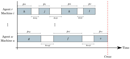
Figure 1.
Graphical representation of the problem.
Alongside the number m of machines, the complexity of parallel machine scheduling problems generally grows exponentially, making large instance problems intractable [3]. In general, the deterministic scheduling problems belong to the category of Combinatorial Optimization problems, many of them are -hard, [40,41]. Likely, -hard complexity problems cannot be solved efficiently by optimization algorithms, requiring exponential time to find an optimal solution, and the development of heuristic algorithms to find a fast solution, by sacrificing optimality [3]. Note that, to define the ASUPM problem, a new variable, agents, is added to the definition of the UPMS problem, conserving the number of machines m, and the number of jobs n, so it is not difficult to see that the ASUPM problem contains the UPMS problem (see Appendix A). As stated in [42,43,44,45], the UPMS problems belongs to the -hard complexity, ergo, the ASUPM is also a -hard problem.
3. Proposed Methods
3.1. Linear Formulations
Six mixed-integer formulations are proposed, which have as foundations the linear models presented by [23] for the unrelated parallel machine scheduling problem with sequence and machine-dependent setup times (UPSM). The model notation is listed below:
- Variable takes 1 if agent r performs job k just after job j in machine i, 0 otherwise.
- Variable takes 1 if agent r performs job k in machine i, 0 otherwise.
- stands for completion time of job j.
- V is used as a large constant.
- is used to denote the set N of n jobs plus a dummy one. All times, both processing and setup associated with the dummy job are 0.
- is used to denote that the job k will be performed first in machine i by agent r.
- is used to denote that the job j will be performed last in machine i by agent r.
Since the problem aims to minimize the maximum makespan, it is needed to linearize the objective function. To do so, the job completion will be used, by stating that all completion times for any job j must be smaller or equal than the maximum makespan .
The first lineal model is stated as:
Objective function (1) minimizes the makespan of the solution. Constraint (2) defines one predecessor to every job, while constraint (3) defines one successor to every job. Constraint (4) ensures that a predecessor and successor of a job are scheduled in the same machine. Constraint (5) ensures the scheduling of the first job with relation one machine to one agent, constraint (6) ensures the scheduling of the first job with relation one agent to one machine. Constraint (7) avoids loops in the processing order, constraint (8) states that the dummy job has no duration. Constraint (9) linearizes the objective function. Finally, constraints (10) and (11) state the nature of variables x and c, respectively.
Furthermore, adding the constraints
Constraint (12) assigns a job to exactly one machine and one agent. Constraint (13) ensures that a predecessor for a job is scheduled in the same machine with the same agent. Constraint (14) ensures that a successor for a job is scheduled in the same machine with the same agent. Constraint (15) defines the nature of y variables.
Let us introduce another way to linearize the objective function, using the span of the machine, . The span is the completion time of the last job in the sequence assigned to the machine i, and for models using variables are defined by expression (16).
Furthermore, the linearization of the objective function by expression (17).
The above expression can be rewritten as:
Additionally, the linearization using variables is defined by:
From the first and second model and considering the linearization by machine span, four extra formulations can be defined:
In the Results section, a comparison is presented between the six formulations proposed to investigate which one produces better results in less computational time.
3.2. Heuristic Algorithms
Due to the -hard complexity of the ASUPM problem, it is impossible, computationally speaking, to solve large instances with mixed-integer linear models, because exponential time is required to find an optimal solution [3]. Hence, a heuristic is proposed to solve the problem in an efficient and faster way, without ensuring optimality. The heuristic is composed of seven algorithms and divided into two categories: Construction of initial solution (designed algorithm) and improvement by intra (tabu search) and inter perturbation (insertions and interchanges). Table 1 presents the maximum number of iterations and the maximum number of iterations without improvement allowed for the heuristic algorithms. The stopping criteria, m, for the Algorithm 1 is directly related to the length p of the job sequence being improved with tabu search, while for Algorithms 2–5, is related to the number of jobs and agents of the instance. In this way, the stopping criteria is not a constant value, but proportional to the size of the instance.
| Algorithm 1: Tabu search |
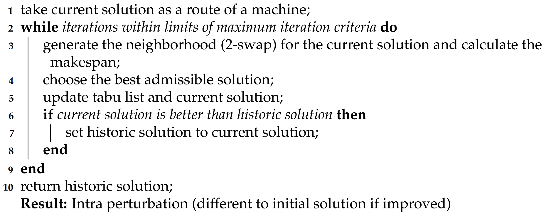 |

Table 1.
Stopping criteria for the algorithms by number of iterations.
| Algorithm 2: Job insertion |
 |
| Algorithm 3: Job interchange |
 |
| Algorithm 4: Job insertion and interchange |
 |
| Algorithm 5: Change of machines |
 |
3.2.1. Constructive Phase
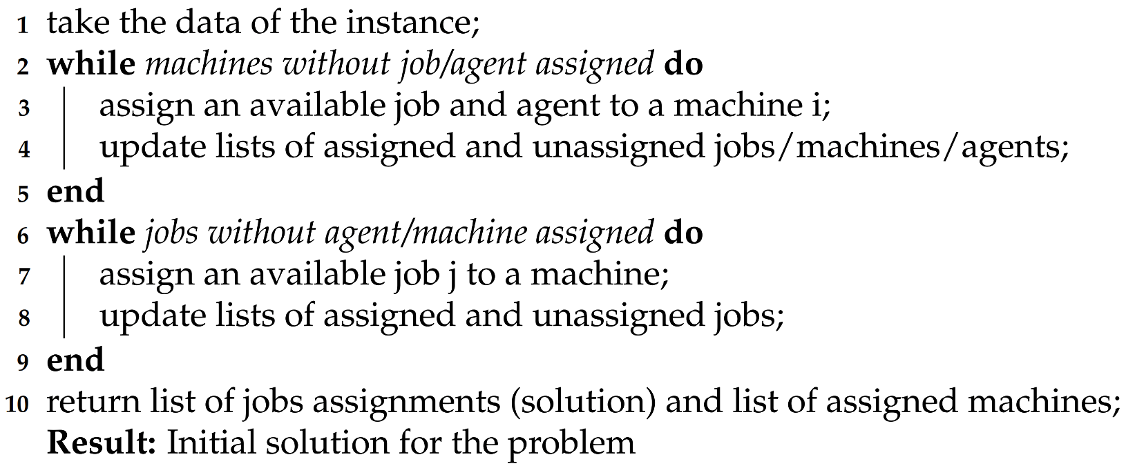
The constructive phase aims to assemble the first sequences of jobs for each agent/machine and provide the improvement phase with a feasible and good solution, which, for different runs, will be different due to the addition of controlled randomness. The pseudo-code of the proposed constructive heuristic is presented in Algorithm 6. Firstly, to initialize the sequences, a machine and an initial job is assigned to each agent. To do so, an unassigned machine is selected randomly. Then, the processing time of performing every available job j in the machine selected is summed, plus the average setup time to perform that job j before any other job available (for the available agents). The job and agent associated with the lowest value are then assigned to the machine selected. The process is repeated until all agents have a machine and an initial job assigned.
| Algorithm 6: Constructive process |
 |
Tabu Search
Later, the sequences of all agents are completed with the unassigned jobs (at this point, the machine assigned to an agent does not change). An unassigned job is selected. The job is inserted at the beginning and the end of every agent’s sequence of jobs. For each insertion, the increment in the makespan is calculated, this will result in values. The jobs are inserted only at the beginning/end to sustain the criteria of insertion based on increments in makespan over the iterations. Then, the values are sorted in ascending order, and a sublist of candidates is created with the first elements (that is, at least one-third of the values will be considered as candidates). A value is randomly selected from the sublist, and the selected job is assigned in the machine and position associated with the value. The process is repeated and finished when all jobs are assigned. The feasible solution is then passed to the improvement algorithms to decrease the maximum makespan of the sequences.
3.2.2. Improvement Phase
The objective of this phase is to minimize as much as possible the maximum makespan of the initial solution, obtained in the constructive phase. To improve the solution, different techniques are used to intra and inter perturb the solution.
Tabu search is used to perform an intra perturbation of a sequence of jobs, that is, improvements within machines. Here, a version is implemented based on the algorithms published in [46]. The pseudo-code of the tabu search implemented is presented in Algorithm 1. In each iteration, a 2-swap neighborhood is evaluated (local search). The 2-swap implies a neighborhood size of , where p is the length of the sequence. For instance, if a sequence of a machine i is given by the jobs , its neighborhood is defined as:
The makespan is calculated for each member of the neighborhood, and the best admissible solution is chosen. The best admissible solution is defined as one in which both members of the pair of jobs swapped are not tabu and increments the less possible (or decreases) the makespan. If the solution is tabu but improves the best solution, it is also chosen (aspiration criteria). The swapped jobs associated with the member of the neighborhood chosen are designed as tabu for the next iterations (proportional to the length of the sequence). That number of iterations is defined as the tabu tenure, which allows avoiding loops around a local minimum. The process is iterated according to Table 1.
Job Insertion
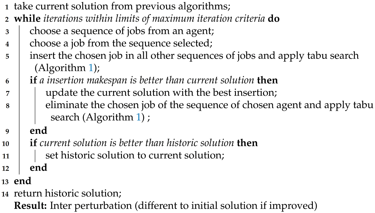
Insertion of jobs is applied to inter perturb the current solution, that is, moving jobs from machines, as presented in the pseudo-code of Algorithm 2. The algorithm is iterated according to Table 1. First, a sequence of jobs of an agent is chosen. An agent is selected randomly, except if the current iteration is multiple of , then the sequence of the busiest agent (more jobs assigned) is chosen, in other words, the busiest agent will be selected each iterations (proportional to the instance size), to balance the jobs assigned within agents, and hence, try to reduce the maximum makespan by letting the agents have a similar workload.
From the selected sequence, a job is chosen randomly. That job is then inserted in all other sequences of jobs, at any position. For each insertion, tabu search is applied, and the makespan is calculated. An insertion is chosen if and only if its makespan is smaller than the maximum makespan of the current solution, and the difference concerning the maximum makespan is the greatest among all insertions. Then, tabu search is applied to the selected sequence (the one that now has one less job), and the current solution is set to the perturbed solution.
As the criteria to choose an insertion only assures that the maximum makespan does not increment, the current solution is compared against the best historical. If the maximum makespan of the current solution is smaller than the maximum makespan of the historic solution, historic is set to current. The algorithm returns the historic solution, different from the initial solution if the insertion technique found a better sequence for the jobs among agents. Note that, at this point, the machines assigned to agents do not change.
Job Interchange
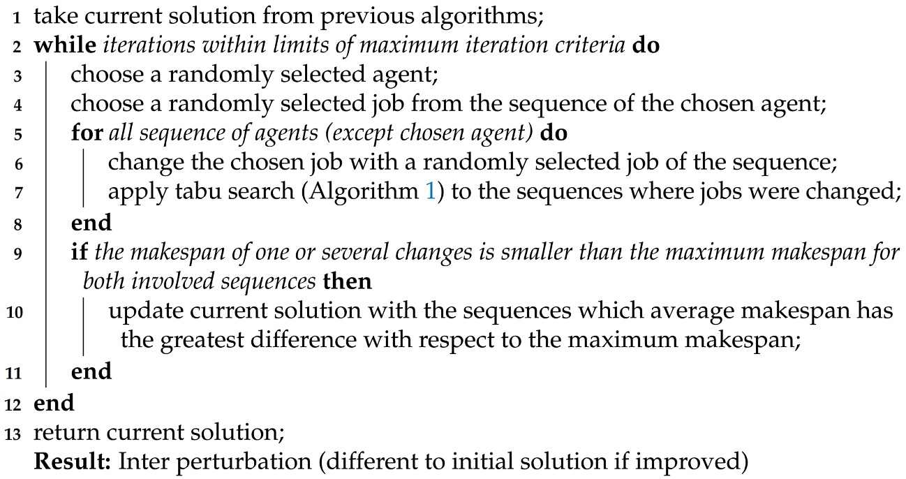
As the insertion of jobs, the job interchange technique is applied to inter perturb the current solution by swapping jobs from machines, as presented in the pseudo-code of Algorithm 3. The logic behind this perturbation technique is: Firstly, from the current solution, a sequence of jobs of an agent is chosen randomly, and a job from this sequence. For all other sequences of jobs, the selected job is swapped with a randomly selected job.
Once the jobs are changed, tabu search is applied in both machines involved in the change and the makespan calculated. A change is chosen if and only if the makespan of the two sequences involved is smaller than the maximum makespan of the current solution, and the average difference concerning the maximum makespan is the greatest among all interchanges. Then, the current solution is set to the perturbed solution, and the algorithm is iterated according to Table 1. The algorithm returns the best solution found, different from the initial solution if the perturbation technique found a better accommodation for the jobs. Still, at this point, the machines assigned to agents do not change.
Job Insertion and Interchange
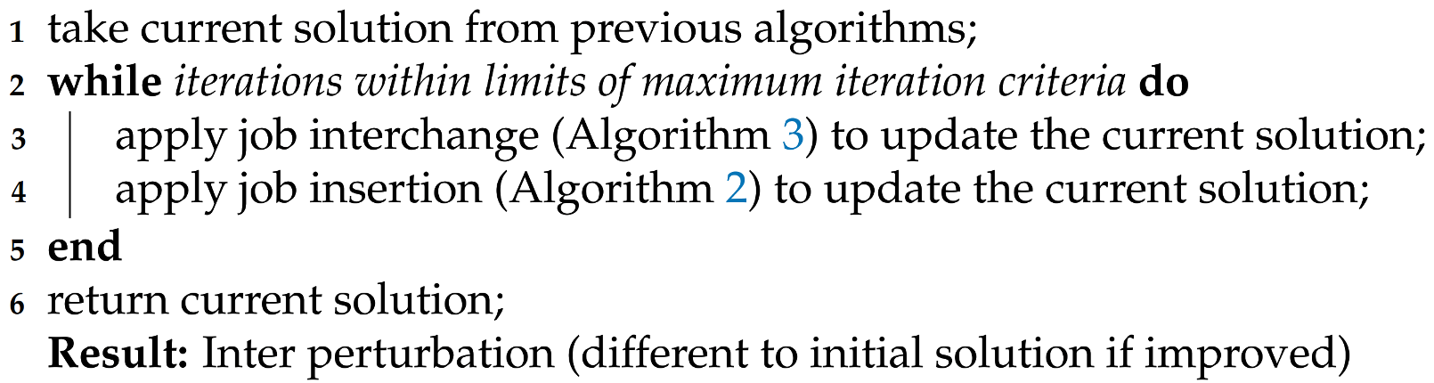
The job insertion and interchange procedure, Algorithm 4, is performed to inter perturb a given solution. To the given solution is applied job interchange (Algorithm 3), and immediately after, job insertion is applied (Algorithm 2). The process is iterated according to Table 1. The algorithm returns the best solution found, different from the initial solution if the perturbation technique found a better accommodation for the jobs. Note that this algorithm does not change machines assigned to agents.
Change of Machines
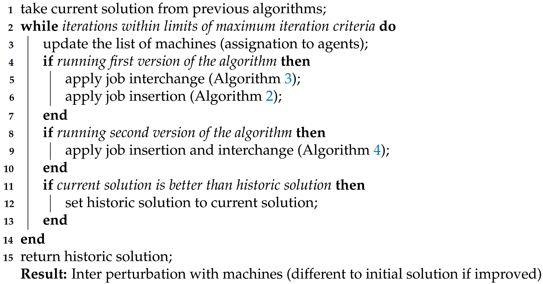
Presented in Algorithm 5, the change of machines procedure is performed to inter perturb the current solution, by changing the machines assigned to agents. The algorithm is iterated according to Table 1.
First, the historic solution is set to the current solution, and it is decided which machines are changed in the current solution. A couple of agents are chosen randomly to swap machines, except if the current iteration is multiple of 4, then all the agents are assigned randomly to any machine. Every 4 iterations, the algorithm will try to reduce the maximum makespan by perturbing all sequences at the same time, involving all agents, machines and jobs. Unlike the other hyperparameters of the other algorithms, which are proportional to the size of the instance, in this case, four iterations were chosen because for the large instances few perturbations were made in all the sequences. In this way, all sequences are constantly disturbed, allowing more solutions to be evaluated.
Then, to the perturbed solution is applied job interchange (Algorithm 3), and to its result job insertion is applied (Algorithm 2), to explore a vast amount of neighborhoods. A second version of the change of machines could be defined, if instead of applying job interchange and insertion, Algorithm 4 is applied, allowing to explore more feasible solutions for a change of machines. After performing the job insertion and interchange, the maximum makespan is compared against the maximum makespan of the historic solution, if it is smaller, historic is set to current. The algorithm returns the historic solution, different from the initial solution if the perturbation technique found a better sequence for the jobs.
3.2.3. Heuristic Conformation
To assembly a heuristic to solve the ASUPM problem, the previously presented algorithms are used in a specific order: depending on the algorithms run, there could be two versions of the heuristic. Both versions are run a fixed amount of time given by the expression (200 ms), where r is the number of agents and n is the number of jobs of the instance being solved. Due to the time criteria to run the algorithm, controlled randomness is applied in all algorithms, since making sequential changes and swaps of jobs/machines by order can cause local searches to skip solutions that reduce significantly the makespan; time could be over before the last elements in the sequences are evaluated.
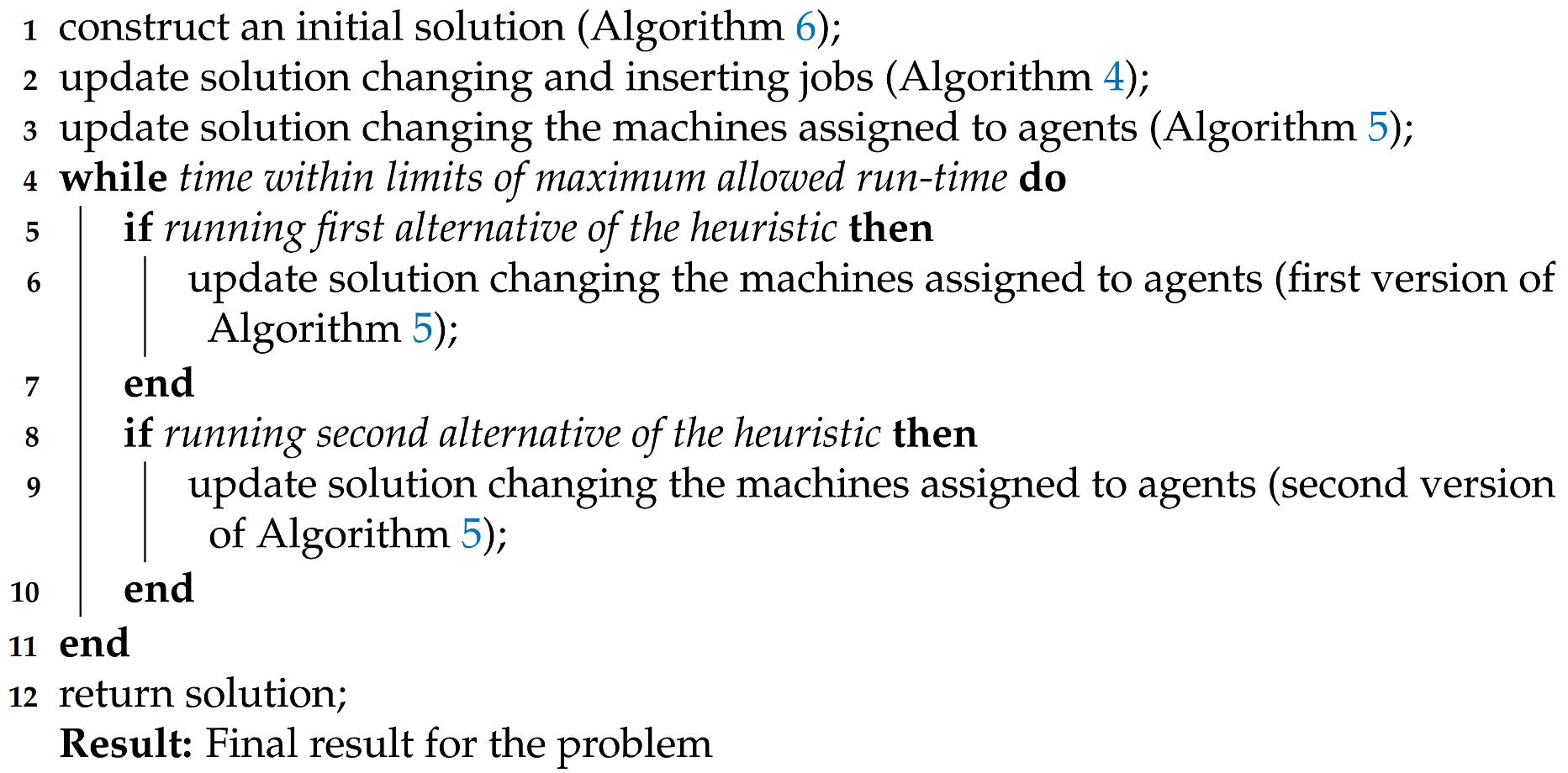
The pseudo-code of the first version of the heuristic is presented in Algorithm 7. To solve the problem, first, it is needed to construct a solution based on the instance data, applying Algorithm 6. Now, with an initial solution available, the solution is improved respecting the assignation of machines to agents by changing and inserting jobs within sequences (Algorithm 4). The solution is further improved by swapping and changing machines to agents, performing the Algorithm 5. From this point and until the time expires, the solution is being improved by the first version of Algorithm 5 if the first alternative of the heuristic is run, and by the second version of Algorithm 5 for the second alternative of the heuristic. When the time is over, the heuristic brings a solution to the problem, which consists of a list of machines assigned to agents, the sequence of jobs of each machine, the list of makespans of each sequence, and the maximum makespan, whose objective was to minimize. Note that, even though the second alternative of the heuristic returns the same elements as the alternative one, it lasts longer for each iteration: for every change of machine more solutions are explored, that is, alternative two can evaluate a greater variety of neighborhoods and their local minima.
| Algorithm 7: Heuristic for the ASUPM problem |
 |
To respect the fluency of reading, an exemplification of the heuristic is presented in the Appendix B section. Additionally, there are presented two application examples in Appendix C: scheduling in the automotive industry and healthcare.
4. Experiments and Results
To test the performance of the solving technique methods proposed, the results of numerical and statistical analysis are obtained for the models and heuristic. To perform the analysis, there were randomly generated instances for the problem, both set-up and processing times with a discrete uniform distribution in the range [1, 99]. To classify an instance by size, it was considered the total data x of the instance, which is given by the expression , which in terms of the number of agents q and the number of jobs n is equivalent to . The size classification of an instance depending on its total data is presented in Table 2.
Table 2.
Instance size based on total data.
4.1. Mixed-Integer Linear Models Results
To compare the performance of the models, the six versions were modeled in Python’s library PuLP, and a small, medium, and large instance were generated and solved with the free-to-use solver COIN CBC 2.10.5 (Coin-Or Foundation Inc., Towson, MD, USA), and the commercial solvers CPLEX V12.10.0.0 (IBM, Armonk, NY, USA) and GUROBI 9.1.1 (Gurobi Optimization, Beaverton, OR, USA). Each possible combination of instance, model, and solver was run ten times. A solution is classified as “unsolved” if one hour of CPU run time passed and the solver could not find the optimal value of the instance. The characteristics of the computer used are Processor Core i5-8265U 1.6 GHz and 8 GB RAM. The summary of run times is presented in Table 3.
Table 3.
Average times (in seconds) for different instances, models and solvers.
To determine which model and solver are the fastest for each one of the three sizes of instances considered, paired two-sample Wilcoxon tests were performed in the programming language R (the values obtained are considered as dependent since the same instance is tested). First, for each size of the instance, it was compared models by pairs for each solver. To do so, the following hypothesis is stated at five percent of significance (let and represent the times to solve an instance for the linear models i and j, where and ):
If the p-value is greater than , the models compared are statistically equal and the comparison ends at this point. Contrarily, if the models are not statistically equal, the comparison is continued and it is stated (at five percent of significance):
If the p-value is smaller than , it is concluded that the run times of model i are smaller concerning the run times of model j. Contrarily, if the p-value is greater than , it is concluded that the run times of model i are greater with respect to the run times of model j. When all comparisons are finished, the count of times model i is smaller with respect to any other model, as is the count of times any other model is greater with respect to model i. The model which has the higher count will be considered as the fastest model for the solver. Then, the fastest model of each solver is compared in the same way to determine the fastest model and solver of the instance. The process is repeated for each one of the three sizes of instances. Since for many of the combinations tested, we did not get an upper bound solution (because the solver reached the time limit or the computer used ran out of memory), and the focus is to determine the fastest model and solver, partial results are not shown.
It was tested a small instance of 2 agents and 10 jobs. According to the unpaired two-sample Wilcoxon tests, for the CBC solver, models four, five, and six are tied in the criteria to determine the fastest model: the count of times these models are smaller concerning to any other model, plus the count of times any other model is greater with respect to these models is one. Since models four, five, and six are statistically equal, it was chosen indiscriminately model four is the fastest model for CBC.
For the CPLEX and GUROBI solvers, the run times of the first five models are statistically greater than model six, hence, model six is chosen as the fastest. Now, the fastest models of each solver are compared similarly in Table 4 through unpaired two-sample Wilcoxon tests. The tests indicate that the run times of model four (CBC) and model six (CPLEX) are statistically greater than the run times of model six (GUROBI). For the small instance, the fastest model is number six, solved with GUROBI.
Table 4.
Comparison of fastest models for each solver to solve a small instance (two agents, ten jobs) with unpaired two-sample Wilcoxon tests.
Additionally, a medium instance of 10 agents and 15 jobs was generated and tested. For the CBC solver, with a score of three, model five is the fastest one, since the count of times it is smaller with respect to any other model is one, and the count of times any other model is greater concerning to it is two. For the CPLEX solver, the run times of the first five models are statistically greater than model six, hence, model six is chosen as the fastest. For the GUROBI solver, models five and six are tied with a score of four. Because models five and six are statistically equal, it was chosen indiscriminately model six as the fastest model for GUROBI. Similarly, the fastest models of each solver are compared in Table 5 through unpaired two-sample Wilcoxon tests. The tests indicate that the run times of model five (CBC) and model six (CPLEX) are statistically greater than the run times of model six (GUROBI). For the medium instance, the fastest model is number six, solved with GUROBI.
Table 5.
Comparison of fastest models for each solver to solve a medium instance (ten agents, fifteen jobs) with unpaired two-sample Wilcoxon tests.
Finally, a large instance of 20 agents and 30 jobs was tested. Since both CBC and CPLEX solvers could not find the optimal value within the one-hour time limit, they are discarded for the analysis to find the fastest model. For the GUROBI solver, the run times of models two to five (model one could not solve the instance within the time limit) are statistically greater than model six, hence, model six is chosen as the fastest. For the large instance, the fastest model is number six, solved with GUROBI.
For the small, medium and large instances tested and considering the imposed time constraint, there is statistical evidence to conclude that the fastest model is model six, solved with GUROBI.
4.2. Heuristic Results
In this section, the two heuristic alternatives are compared to each other, as well as the best results obtained against many optimal values for generated instances. The algorithms that integrate the heuristic were programmed in Python 3.
4.2.1. Comparison of Heuristics
Paired two-sample Wilcoxon tests were performed in the programming language R to compare the performance of the two heuristic alternatives for a small, medium and a large instance (same instances used in the previous section). Even though both heuristics are different, and the results of the alternative one are not affected by the results of the second alternative, results are considered dependent since we are comparing heuristics by the same instance. Let A denote the population of alternative one of the heuristic and B the population of alternative two. First, to determine if the values of A are equal to the values of B, it is stated:
If there is enough statistical evidence to reject the null hypothesis, we may expect that values from alternative two are smaller than the ones from version one, so it is stated:
All tests were made with a significance level of five percent and a sample size of ten for each population. Table 6 shows the codes of each stage of the heuristic presented in Figure 2, Figure 3 and Figure 4.
Table 6.
Stage codes of the heuristic.
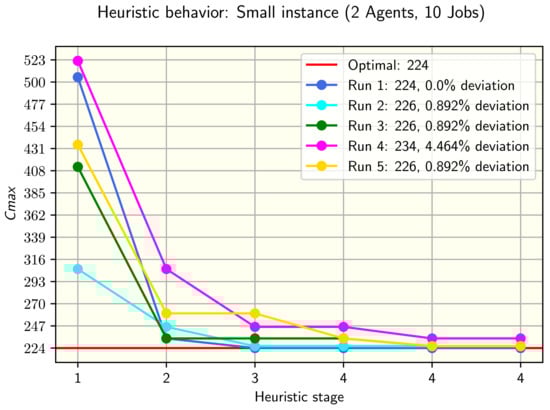
Figure 2.
Five runs and its results for a small instance in alternative two.
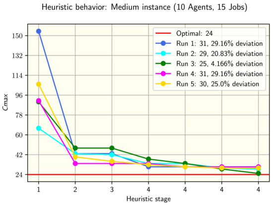
Figure 3.
Five runs and its results for a medium instance in alternative two.
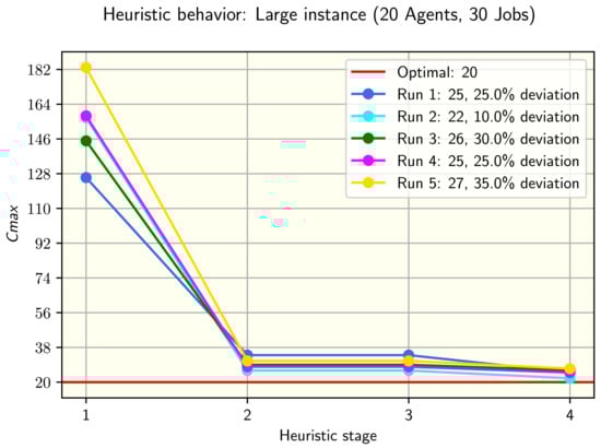
Figure 4.
Five runs and its results for a large instance in alternative two.
For the small instance (2 agents and 10 jobs), after the Wilcoxon test to determine if the values obtained from alternatives one and two of the heuristic are equal, the null hypothesis was failed to reject, so we conclude that the values are not significantly different. Figure 2 shows five runs of the heuristic for the instance tested.
For the medium instance (10 agents and 15 jobs), it was rejected the null hypothesis of the Wilcoxon test to determine if the values obtained from alternatives one and two of the heuristic are equal. The process is continued, by testing if the values from alternative two are greater or equal than those from alternative one. The null hypothesis is also rejected, so it is concluded that the values obtained from alternative two are significantly smaller. Figure 3 shows five runs of the heuristic for the instance tested.
Finally, for the large instance (20 agents, 30 jobs), there was enough statistical evidence to conclude that the values obtained from alternatives one and two of the heuristic are not equal. Continuing with the comparisons, it was tested if the values from alternative two are greater or equal than those from alternative one. The null hypothesis is also rejected, so it is concluded that the values obtained from alternative two are significantly smaller. Figure 4 shows five runs of the heuristic for the instance tested.
For the small instance, there is no statistical evidence to conclude that the versions of the heuristic give different results. For the medium and large instances, there is enough evidence to conclude that version two gives better results than version one. A summary of the comparisons is presented in Table 7.
Table 7.
Summary of Wilcoxon tests to compare the alternatives of the heuristic.
4.2.2. Performance of the Heuristic: Comparison against Optimal Values
A set of instances was generated considering the following combinations of number of agents r and number of jobs n: , where z represents the agent in the r set being combined. The instances generated were classified according to Table 2. The heuristic was run at most three times, and the instances for which the optimal value could not be found with model six and GUROBI within one hour of CPU run time or due to lack of memory of the computer used were not considered. To complete 100 instances of each size, some second versions of the considered instances were generated (the selection of a considered instance was made randomly). Table 8 presents the results of alternative two of the heuristic applied to the generated instances for which the optimal value is known. The gap and relative deviation for a given instance i were calculated in the expressions (20) and (21), respectively.
Table 8.
Summary of the heuristic performance for generated instances.
Figure 5a and Figure 6a show the relative deviations and gaps obtained for small instances. Only for six instances, the optimal value could not be found, representing less than 1% of relative deviation. The average gap between the optimal and best-obtained values is almost zero, which indicates that for small instances, the heuristic performs very well.
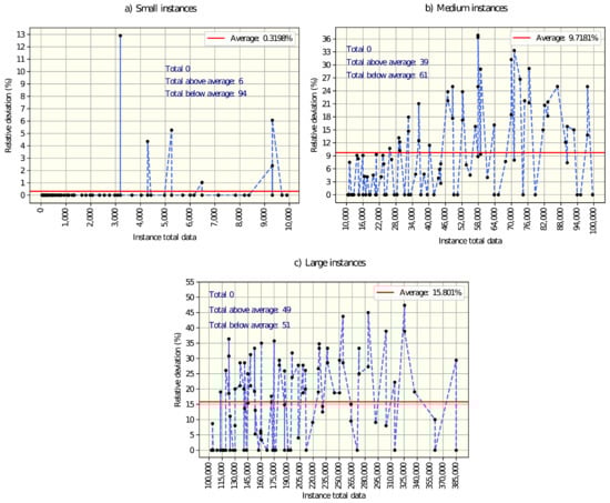
Figure 5.
Relative deviation for: (a) Small, (b) Medium and (c) Large instances.
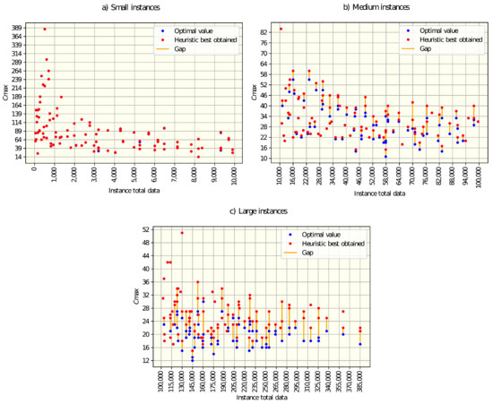
Figure 6.
Differences between optimal and the best heuristic value for: (a) Small, (b) Medium and (c) Large instances.
Now, it turns to analyzing the medium instances. Figure 5b and Figure 6b show the deviations and gaps obtained for that size of instances. 61% of the instances presented a relative deviation below the average (9.71%). The gaps between the optimal and best-obtained values are larger in comparison with small instances, but on average are close to zero (2.69). For medium instances, the heuristic had a good performance.
Finally, let us analyze the results obtained for large instances. Figure 5c and Figure 6c show the deviations and gaps obtained. This time, around half the instances are below the average relative deviation, which is 15.8%. The gaps with respect to optimal values are on average greater than the gap for small and medium instances, and just 30 instances were solved to optimality. The heuristic presented an acceptable performance for large instances.
5. Discussion and Conclusions
The proposed model allows depicting a more integral scenario of productive systems where individual attention is needed for each machine. Along with the management of tasks and processes, the model incorporates the subject that can be a person, a robot, or any entity in charge of operating these machines. Using a service process as an example, the model can be used as a tool for employee management (if subjects are people), which could lead to an increase in customer satisfaction if the makespan, and hence the time to finish the services, are minimized.
There is a significant difference in the performance (time) to find an optimal value between the linear models proposed in this study. In general, the models that linearize the objective function by the machine span are faster than the models that linearize it by the job completion time; however, the model that considers both types of linearization and uses two index binary variables is the fastest. Similarly, there is a clear difference between commercial and free-to-use optimizers, while the free-to-use optimizer used in this research is slow and tends to be unstable for large instances, GUROBI presented the fastest times to solve different sizes of instances, although the differences with respect to CPLEX are not large.
The -hard complexity of the problem is easily experienced when dealing with large instances since the computer runs out of memory before even finding a lower bound for the objective function. Here is where heuristic algorithms gain relevance. The heuristics are recommended to use when dealing with medium, but especially with large instances, as the solvers can take too long to converge to optimality, and even before the computer used can run out of memory. The performance difference between the two heuristics proposed is evident for large instances, where the number of feasible solutions is high. Hence, the second heuristic outperforms the first, given the exploration of more neighborhoods (more possibilities to find a solution) for each machine change. In general, the proposed heuristic will find a solution faster than the solvers, and has an outstanding performance in small instances, since it can find the optimal value for almost every instance, very good behavior in medium instances, and decent performance for large instances, where the relative deviations tend to increase with respect to the small and medium instances. Broadly, the heuristics perform well, for any size of the instance, if the relation of jobs assigned to machines is low because it can explore more neighborhoods (solutions), due to the nested improvement stage.
The problem addressed in this research mathematically includes the assignation models where the dimension of decision variables is lower than the variables of the ASUPM problem. The instances of those previous problems can be adapted and solved with the models and heuristic proposed in this study. For example, the heuristic presented could solve a problem of parallel machines and sequence-dependent times without agents, as well as the problem with identical machines and fixed processing and setup times. However, solving these sub-problems with the ASUPM methods would be computationally inefficient because the duplicated data would result in exploring repeated neighborhoods.
Different real-world applications can be found in the industry and services. The model could be applied in any process where a subject performs a task in a workstation/machine, with or without an object in the machine. The application of models like the ASUPM will allow companies to better manage their processes and resources by reducing assignment costs or increasing the utilization of machines and resources to become more competitive. Nonetheless, in real-life scenarios, a tolerance based on the nature of the application must be defined to calibrate the algorithms with instances for which the optimal/best values are known, before applying the heuristic.
Because the ASUPM is a -hard problem, a great opportunity for future research is the development of models and algorithms that overperform the presented in this paper. Additionally, future works should add more realistic elements such as Maintenance activities, energy consumption, inventories, resources in the process, work shifts, and/or just-in-time criteria.
Author Contributions
Conceptualization, J.I.V.-S. and L.E.C.-B.; Data curation, J.I.V.-S.; Formal analysis, J.I.V.-S.; Investigation, J.I.V.-S., L.E.C.-B. and R.E.P.-G.; Methodology, J.I.V.-S., L.E.C.-B. and R.E.P.-G.; Project administration, J.I.V.-S., L.E.C.-B. and R.E.P.-G.; Resources, J.I.V.-S., L.E.C.-B. and R.E.P.-G.; Software, J.I.V.-S.; Supervision, L.E.C.-B. and R.E.P.-G.; Validation, J.I.V.-S., L.E.C.-B. and R.E.P.-G.; Visualization, J.I.V.-S.; Writing—original draft, J.I.V.-S.; Writing—review & editing, J.I.V.-S., L.E.C.-B. All authors have read and agreed to the published version of the manuscript.
Funding
This research received no external funding.
Institutional Review Board Statement
Not applicable.
Informed Consent Statement
Not applicable.
Data Availability Statement
The data used in this research, such as the instances and their best-known values are available to interested readers at a01262327@itesm.mx.
Conflicts of Interest
The authors declare no conflict of interest.
Abbreviations
The following abbreviations are used in this manuscript:
| ASUPM | Agent scheduling in unrelated parallel machines with sequence and agent–machine dependent setup times |
| UPMS | Unrelated parallel machines scheduling with sequence and machine-dependent setup times |
Appendix A. Contention of the UPMS in the ASUPM Problem
The UPMS problem belongs to the -hard complexity. To demonstrate that the ASUPM problem is also -hard, it is needed to show that the ASUPM contains the UPMS problem.
Let us recall that the UPMS problem aims to schedule jobs to machines while minimizing the maximum makespan, and has as model parameters the processing time of job k in machine i, and the setup times to perform job k right after job j in machine i, . To perform the demonstration, let us show that a UPMS instance could be adapted and solved by the ASUPM defined techniques.
Let A be the variables, parameters and assumptions of the UPMS problem, x a valid (in terms of size and content) instance for the UPMS problem with optimal value Z, B the variables, parameters and assumptions of the ASUPM problem and y a valid instance for the ASUPM problem with optimal value W. Since to the definition of the UPMS problem a new variable is added, agents, conserving the number of machines, m, and the number of jobs n, so it is stated:
Lemma A1.
The ASUPM problem contains the UPMS problem.
Theorem A1.
For any valid instance of the UPMS problem, x, exists a valid instance for the ASUPM problem, y, composed of x in such a way that the solution to x and y is the same.
Proof.
To prove the theorem, let us first calculate the total number of data of a given instance x for the UPMS problem. We know there is processing times , and sequence-dependent setup times , where i is the index corresponding to the set of m machines, and j and k the indexes of the set of n jobs. By multiplying the number of elements in the sets associated with the indexes, we can obatin the total data:
To calculate the total data for a given instance y for the ASUPM problem, we add to the equation the number q of agents:
Because there is a machine for every agent, we can substitute q by m:
Now, the data difference between instances is calculated:
Coming back to the demonstration, let us recall the setup times definition for the UPMS problem: there is a different time to setup job j before job k for every machine ( represents a matrix with the setup times to perform job j before job k, that is, a matrix of size , with total data equal to ):
Let S be the set of all matrix, so m has a matrix of size , that is, a total data of . The set S, alongside the processing times, have an optimal value of Z for the UPMS problem. Now, the only way in which the optimal value Z is equal to the optimal value W of the ASUPM problem is if and only if the numbers of the instance are the same. Since, as presented above, the total data of the ASUPM problem instance, , is greater than the total data of the UPMS instance , even if we use the same data of the x instance for the y instance, we are missing data, the data corresponding to the new variable, agents. Because there is a relation one agent to one machine, for each agent, the information of the setup times for each machine is needed in order to duplicate data to obtain a valid ASUPM problem instance (please note that, for both UPMS and ASUPM problems, the processing times will be the same, because a machine i always lasts the same performing job j, no matter the agent in charge of the machine):
Let be the set of all S, so now has a matrix of size , that is, a total data of . Then, the total data difference is calculated between the UPMS and ASUPM instances. The processing time can be ignored for the difference calculation since it is a constant matrix:
The relation holds, so the instance created by duplicating data from the UPMS instance is valid for the ASUPM problem. Now it is time to check if the instances have the same optimal value. The set S of the UPMS problem valid instance has an optimal value Z:
In the valid ASUPM instance, we have a set composed of a q number of S, since we duplicated data:
Each of the elements of has a local optima value, which is the same for all elements, and turns out to be Z. The repeated local optima transfer into the global optima of the instance, W, so , the instances have the same optimal value.
A UPMS instance can be adapted and solved by the ASUPM defined techniques, ergo, the ASUPM contains the UPMS problem. □
Appendix B. Heuristic Exemplification
Let us suppose we have an instance of 2 agents and 8 jobs that needs to be solved with the heuristic proposed, whose processing times are (note that some values are colored, these values will be helpful to identify the numbers used in the logic processes):
Furthermore, set-up times:
Appendix B.1. Construction of the Initial Solution
An initial solution will be constructed with the Algorithm 6. First, an available machine is randomly selected, let us choose machine 2. The next step is, to sum the processing times of performing each of the 8 available jobs in machine 2, plus the average setup time to perform each job before any other. For instance, to evaluate the time it takes for job 4 to be processed in machine 2 by agent 1, we perform: .
From the computation, the minimum total time value, 78.1429, corresponds to agent 1 and job 2, so agent 1 is assigned machine 2 and job 2. Then, the process is continued; since machine 1 is the only one available, it is selected. Similarly, the sum of processing times and average setup times are computed for machine 1 and the jobs and agent available; after the computations, with a value of 60.2857, machine 1 and job 5 are assigned to agent 2.
The sequences must be completed by assigning all available jobs (1, 3, 4, 6, 7, 8). To do so, a job is randomly selected, let us pick job 6. This job is inserted at the beginning and the end of the sequences of agents 1 (job 2) and 2 (job 5), and the increment in the makespan is calculated for each insertion.
First, let us start evaluating the insertion at the beginning of the sequence of agent 1, that is, the sequence of jobs 6-2. The increment in the makespan is calculated summing the processing time of job 6 in machine 2 plus the setup time of performing job 2 after 6 in machine 2 by agent 1, .
The next step is to evaluate the insertion of job 6 at the end of the jobs assigned to agent 1, sequence 2-6. The increment in the makespan is the sum of the processing time of job 6 in machine 2 plus the setup time of performing job 6 after 2 in machine 2 by agent 1, .
Let us evaluate the insertion in the sequence of agent two, first at the beginning, resulting in sequences 6-5. The makespan increment is the sum of the processing time of job 6 in machine 1 plus the setup time of performing job 5 after 6 in machine 1 by agent 2, .
It is turning to evaluate the insertion of job 6 at the end of jobs assigned to agent 2, sequence 5-6. The increment in the makespan is the sum of the processing time of job 6 in machine 1, plus the setup time of performing job 6 after 5 in machine 1 by agent 2, .
Now, we have 4 values: 87, 93, 132, 150. The values are sorted in ascending order, in this case, the values are already ordered. Only the first values are considered for a subsequent sublist of candidates, which are 87, 93. A member of the list of candidates is selected randomly, let us choose 93. Since the 93 value is associated with agent 1 at the end position, job 6 is added to the now new sequence of jobs 2-6, assigned to agent 1 and machine 2. The process is repeated until all 5 remaining jobs are assigned to a sequence. Continuing with the Algorithm 6, an initial solution is obtained: Agent 1, machine 2, jobs 2-6-8-3; Agent 2, machine 1, jobs 4-7-5-1, with maximum makespan equal to 268.
Appendix B.2. Improvement by Inserting and Changing Jobs
When an initial solution is constructed, is then time to improve this solution, first by changing and inserting jobs, according to Algorithm 4. Remember the current solution: Agent 1, machine 2, jobs 2-6-8-3; Agent 2, machine 1, jobs 4-7-5-1, with maximum makespan 268.
To the current solution, first the change of jobs procedure is applied, presented in Algorithm 3. According to this algorithm, first an agent is selected randomly. Let us pick agent 2. Now, a job is randomly selected and extracted from the sequence of agent 2, let us choose job 5, which leads to the sequence 4-7-1 of agent 2. For all other sequences of jobs, job 5 is swapped with a randomly selected job. Since there is only one remaining sequence of jobs (sequence of agent 1), job 3 of this sequence is selected (randomly) and extracted, leading to the sequence 2-6-8 of agent 1. Now, the extracted jobs are swapped, resulting in the sequence 2-6-8-5 for agent 1 and sequence 4-7-3-1 for agent 2. For the new sequences, tabu search, Algorithm 1, is applied. Let us evaluate the application of tabu search in the sequence 2-6-8-5 of agent 1, whose makespan is 311 (set initial to historic solution). Firstly, for each of the neighborhoods of the current solution the makespan is calculated (tabu search iteration 1):
6-2-8-5; swapped 6 and 2, makespan equal to 348.
8-6-2-5; swapped 8 and 2, makespan equal to 330.
5-6-8-2; swapped 5 and 2, makespan equal to 304.
2-8-6-5; swapped 8 and 6, makespan equal to 308.
2-5-8-6; swapped 5 and 6, makespan equal to 358.
2-6-5-8; swapped 5 and 8, makespan equal to 330.
8-6-2-5; swapped 8 and 2, makespan equal to 330.
5-6-8-2; swapped 5 and 2, makespan equal to 304.
2-8-6-5; swapped 8 and 6, makespan equal to 308.
2-5-8-6; swapped 5 and 6, makespan equal to 358.
2-6-5-8; swapped 5 and 8, makespan equal to 330.
With makespan equal to 304, the sequence 5-6-8-2 is selected, since it is the option the reduces the most the makespan. In addition, the selected sequence is set as the historic solution, because its makespan is smaller than the initial solution. The tabu tenure is defined as , where n is the number of elements in the sequence being evaluated. The swap of jobs 5-2 will be tabu for the next tabu tenure iterations (2), that is, until iteration 3. The makespan is calculated for each of the neighborhoods of the selected sequence (tabu iteration 2):
6-5-8-2; swapped 6 and 5, makespan equal to 340.
8-6-5-2; swapped 8 and 5, makespan equal to 270.
2-6-8-5; swapped 2 and 5, makespan equal to 311.
5-8-6-2; swapped 8 and 6, makespan equal to 329.
5-2-8-6; swapped 2 and 6, makespan equal to 303.
5-6-2-8; swapped 2 and 8, makespan equal to 331.
8-6-5-2; swapped 8 and 5, makespan equal to 270.
2-6-8-5; swapped 2 and 5, makespan equal to 311.
5-8-6-2; swapped 8 and 6, makespan equal to 329.
5-2-8-6; swapped 2 and 6, makespan equal to 303.
5-6-2-8; swapped 2 and 8, makespan equal to 331.
The sequence 8-6-5-2, with makespan 270 is selected since it reduces the most makespan. This sequence is set as the historic solution, because its makespan is smaller than the previous historic of 304. The tabu list (in terms of the number of iteration) is {(5-2): 3, (8-5): 4}. The neighborhood is defined as (tabu iteration 3):
6-8-5-2; swapped 6 and 8, makespan equal to 287.
5-6-8-2; swapped 5 and 8, makespan equal to 304 (is tabu).
2-6-5-8; swapped 2 and 8, makespan equal to 330.
8-5-6-2; swapped 5 and 6, makespan equal to 330.
8-2-5-6; swapped 2 and 6, makespan equal to 356.
8-6-2-5; swapped 2 and 5, makespan equal to 330 (is tabu).
5-6-8-2; swapped 5 and 8, makespan equal to 304 (is tabu).
2-6-5-8; swapped 2 and 8, makespan equal to 330.
8-5-6-2; swapped 5 and 6, makespan equal to 330.
8-2-5-6; swapped 2 and 6, makespan equal to 356.
8-6-2-5; swapped 2 and 5, makespan equal to 330 (is tabu).
Note that two sequences were tabu, which means they cannot be selected, except, by the aspiration criteria, if its makespan is smaller than 270 (historic smallest in tabu search), but this is not the case. None of the options reduce the makespan, so, the sequence 6-8-5-2 is selected since its makespan, 287, increases the least the makespan and it is not tabu. The tabu list is updated, {(8-5): 4, (6,8): 5}, and the neighborhood for the current solution is evaluated (tabu iteration 4):
8-6-5-2; swapped 8 and 6, makespan equal to 270 (is tabu).
5-8-6-2; swapped 5 and 6, makespan equal to 329.
2-8-5-6; swapped 2 and 6, makespan equal to 350.
6-5-8-2; swapped 5 and 8, makespan equal to 340 (is tabu).
6-2-5-8; swapped 2 and 8, makespan equal to 366.
6-8-2-5; swapped 2 and 5, makespan equal to 331.
5-8-6-2; swapped 5 and 6, makespan equal to 329.
2-8-5-6; swapped 2 and 6, makespan equal to 350.
6-5-8-2; swapped 5 and 8, makespan equal to 340 (is tabu).
6-2-5-8; swapped 2 and 8, makespan equal to 366.
6-8-2-5; swapped 2 and 5, makespan equal to 331.
Note that we have a sequence with a makespan of 270, this reduces the most the makespan, but, being tabu, and being not smaller than the historic smallest in tabu search, is not chosen. The best admissible sequence is 5-8-6-2, with a makespan of 329. The subsequent results of the tabu search are presented below.
Tabu iteration 5, current solution 5-8-6-2, makespan 329. Tabu list {(6,8): 5, (5,6): 6}. Neighborhoods:
8-5-6-2; swapped 8 and 5, makespan equal to 330.
6-8-5-2; swapped 6 and 5, makespan equal to 287 (is tabu).
2-8-6-5; swapped 2 and 5, makespan equal to 308.
5-6-8-2; swapped 6 and 8, makespan equal to 304 (is tabu).
5-2-6-8; swapped 2 and 8, makespan equal to 274.
5-8-2-6; swapped 2 and 6, makespan equal to 359.
6-8-5-2; swapped 6 and 5, makespan equal to 287 (is tabu).
2-8-6-5; swapped 2 and 5, makespan equal to 308.
5-6-8-2; swapped 6 and 8, makespan equal to 304 (is tabu).
5-2-6-8; swapped 2 and 8, makespan equal to 274.
5-8-2-6; swapped 2 and 6, makespan equal to 359.
Tabu iteration 6, current solution 5-2-6-8, makespan 274. Tabu list {(5,6): 6, (2,8): 7}. Neighborhoods:
2-5-6-8; swapped 2 and 5, makespan equal to 317.
6-2-5-8; swapped 6 and 5, makespan equal to 366 (is tabu).
8-2-6-5; swapped 8 and 5, makespan equal to 318.
5-6-2-8; swapped 6 and 2, makespan equal to 331.
5-8-6-2; swapped 8 and 2, makespan equal to 329 (is tabu).
5-2-8-6; swapped 8 and 6, makespan equal to 303.
6-2-5-8; swapped 6 and 5, makespan equal to 366 (is tabu).
8-2-6-5; swapped 8 and 5, makespan equal to 318.
5-6-2-8; swapped 6 and 2, makespan equal to 331.
5-8-6-2; swapped 8 and 2, makespan equal to 329 (is tabu).
5-2-8-6; swapped 8 and 6, makespan equal to 303.
The number of maximum iterations for the tabu search is defined by , and the number of maximum iterations without improvement by . The best solution in the tabu search was, with a makespan of 270, the sequence 8-6-5-2, found in iteration 2. Four iterations passed without improvement (iteration 3, 4, 5 and 6), so the tabu search finishes at this point, returning the best solution.
Back to the change of jobs procedure, Algorithm 3, we applied tabu search to the sequence 2-6-8-5 of agent 1, resulting in 8-6-5-2 with a makespan of 270. We need to apply tabu search to the sequence of agent 2, 4-7-3-1. If we apply tabu search according to the criteria defined above, the sequence 3-1-4-7 is obtained, with a makespan of 221. Since one of the solutions obtained in the tabu search is greater than the maximum makespan of the global current solution, 268, the new sequences are discarded and a new iteration of Algorithm 3, change of jobs, is started.
From the current global solution, Agent 1, machine 2, jobs 2-6-8-3; Agent 2, machine 1, jobs 4-7-5-1, with maximum makespan 268, an agent is selected randomly, let us pick agent 1. From the sequence of agent 1, a job is randomly selected and extracted, let us choose job 3, obtaining the sequence 2-6-8. From the remaining sequence, agent 1, a job is randomly selected and extracted, let us pick job 4, resulting in sequence 7-5-1. The extracted jobs are swapped, resulting in sequence 2-6-8-4 for agent 1, and sequence 7-5-1-3 for agent 2. If we apply tabu search to both sequences, for agent 1, the sequence 6-8-4-2 is obtained, with a makespan of 243, and sequence 7-5-3-1, with a makespan of 162, for agent 2. Since both makespans are smaller than the maximum makespan of the global current solution, 268, the new sequences obtained are set to the current solution.
As stated before, the number of maximum iterations for the change of jobs procedure is defined by , and number of maximum iterations without improvement by . Continuing with the computations, the best solution is found in iteration 2, with a maximum makespan of 243, four iterations passed without improvement (iteration 3, 4, 5 and 6), so the change of jobs technique finishes at this point, with a solution: Agent 1, machine 2, jobs 6-8-4-2; Agent 2, machine 1, jobs 7-5-3-1, with maximum makespan 243.
The next step in the changing and inserting jobs procedure is to perform the Algorithm 2, job insertion, to the solution found in the change of jobs procedure (Algorithm 3). First, an agent is chosen randomly, except every iterations, when the busiest agent (the one with more jobs assigned) is selected. Since this will be the first iteration, let us make a random choice, agent 1. After, a job from the sequence of the selected agent is chosen randomly, let us pick job 2. Job 2 is then inserted in all other sequences of jobs, at any position. For each insertion, tabu search is applied; since the only sequence remaining is the sequence of jobs of agent 2, there will be only one insertion per iteration. Job 2 is inserted in the sequence of agent 2, resulting in 7-5-3-1-2. To this sequence tabu search is applied, obtaining 1-5-3-2-7, with a makespan of 172. Because the makespan obtained is smaller than the maximum makespan of the current global solution, 243, we keep the insertion. Then, tabu search is applied to the sequence of agent 1, where job 2 was removed: 6-8-4. Tabu search gives the sequence 6-8-4 as a solution, with a makespan of 203. The solution: Agent 1, machine 2, jobs 6-8-4; Agent 2, machine 1, jobs 1-5-3-2-7, with maximum makespan 203 is set to the current and historic solution since it reduces the global maximum makespan.
For the next iteration, the second one, let us pick agent 2, and job 1 from its sequence of jobs. Job 1 is inserted in the sequence of agent 1, resulting in 6-8-4-1. After tabu search, the sequence 1-6-8-4 is obtained, with a makespan of 269. The maximum makespan of the current solution is 203, so the insertion is discarded because it makes the solution worse.
The number of maximum iterations for the change of jobs procedure is defined by , and number of maximum iterations without improvement by . The best solution is found in the first iteration, and according to further computations, insertions in iterations 3, 4 and 5 did not improve and update the current solution, as four iterations passed without improvement, the job insertion algorithm finishes at this point. In addition, job insertion and interchange, Algorithm 4, is finished now, with the solution: Agent 1, machine 2, jobs 6-8-4; Agent 2, machine 1, jobs 1-5-3-2-7, with maximum makespan 203.
Appendix B.3. Improvement by Changing of Machines
The improvement by changing and inserting jobs respected the initial assignation of machines to agents, this time, further solutions will be evaluated by changing machines, according to Algorithm 5. First, the current solution is set to the historic solution (Agent 1, machine 2, jobs 6-8-4; Agent 2, machine 1, jobs 1-5-3-2-7, with maximum makespan 203). To develop the perturbation technique, it is needed to update the list of machines by choosing randomly a couple of agents and changing their assigned machines, except if the current iterations are multiple of 4, then all agents will be assigned a machine randomly. Since this is the first iteration, let us choose agent 1 and change its machine with agent 2, so, the assignations of machines and jobs to evaluate are: Agent 1, machine 1 jobs 6-8-4; Agent 2, machine 2, jobs 1-5-3-2-7. To this solution, is then applied the job interchange technique explained previously (Algorithm 3), to obtain the solution: Agent 1, machine 1, jobs 1-5-4; Agent 2, machine 2, jobs 8-6-3-7-2, with a maximum makespan of 279. To this solution, the job insertion technique explained above is applied (Algorithm 2). After the procedure, a solution is obtained: Agent 1, machine 1, jobs 5-4-8-1; Agent 2, machine 2, jobs 6-3-7-2, with a maximum makespan of 241. Since the maximum makespan of the perturbed solution is greater than the historic maximum makespan (203), it makes the solution worse, the assignation is discarded and a new iteration is started.
For the second iteration, let us pick agent 2, and change its machine with agent 1, to evaluate the solution: Agent 1, machine 1, jobs 6-8-4; Agent 2, machine 2, jobs 1-5-3-2-7. After the application of the job interchange technique, the solution is obtained: Agent 1, machine 1, jobs 5-3-7; Agent 2, machine 2, jobs 8-6-1-4-2, with maximum makespan 327. To this solution the job insertion technique is applied to obtain the solution: Agent 1, machine 1, jobs 8-3-7-1-5; Agent 2, machine 2, jobs 4-2-6, with maximum makespan 196. The solution obtained in this iteration reduces the maximum makespan of 7 units with respect to the historic solution, so we set the found assignation as the historic solution.
Similarly to other algorithms, the number of maximum iterations for the change of machines procedure is defined by , and number of maximum iterations without improvement by . If the computations are continued, the best solution is found in the second iteration, the changes of machines in iterations 3, 4, 5 and 6 did not improve and update the current solution, as four iterations passed without improvement, the algorithm finishes at this point, with the historic solution: Agent 1, machine 1, jobs 8-3-7-1-5; Agent 2, machine 2, jobs 4-2-6, with maximum makespan 196.
For both of the alternatives of the heuristic, the first iteration is completed with Algorithm 5, and further iterations will continue to improve the solution by changing machines. However, for the second alternative of the heuristic, the improvement is made with the second version of the changing of machines procedure (Algorithm 5). The difference is stated after the new assignation of machines, where instead of applying Algorithms 2 and 3, Algorithm 4 is applied. Because the second change of machines procedure, (Algorithm 5), is composed of algorithms that were already exemplified, the details of its application are not shown.
Appendix B.4. Final Results of the Heuristics for the Instance Being Solved
There are presented in Table A1 the summary of results of the two versions of the heuristic for the instance being solved. Let us remember that the solution after the first iteration is (which is the same for both versions): Agent 1, machine 1, jobs 8-3-7-1-5; Agent 2, machine 2, jobs 4-2-6, with maximum makespan 196. The optimal maximum makespan for the instance is 185.
Table A1.
Summary of results, two alternatives of the heuristic.
Table A1.
Summary of results, two alternatives of the heuristic.
| Heuristic Version 1 | Heuristic Version 2 | ||||
|---|---|---|---|---|---|
| Iteration | Algorithm | Max Makespan | Iteration | Algorithm | MaxMakespan |
| 1 | Algorithm 6 (constructive) | 268 | 1 | Algorithm 6 (constructive) | 268 |
| Algorithm 4 (change, insert jobs) | 203 | Algorithm 4 (change, insert jobs) | 203 | ||
| Algorithm 5 (change machines) | 196 | Algorithm 5 (change machines) | 196 | ||
| 2 | Algorithm 5 (change machines) | 196 | 2 | Algorithm 5 (change machines, second version) | 194 |
| 3 | Algorithm 5 (change machines) | 196 | 3 | Algorithm 5 (change machines, second version) | 185 |
| ⋮ | ⋮ | ⋮ | 4 | Algorithm 5 (change machines, second version) | 185 |
| 23 | Algorithm 5 (change machines) | 194 | ⋮ | ⋮ | ⋮ |
| 24 | Algorithm 5 (change machines) | 194 | 10 | Algorithm 5 (change machines, second version) | 185 |
| ⋮ | ⋮ | ⋮ | |||
| 29 | Algorithm 5 (change machines) | 185 | |||
| 30 | Algorithm 5 (change machines) | 185 | |||
| ⋮ | ⋮ | ⋮ | |||
| 46 | Algorithm 5 (change machines) | 185 | |||
The optimal solution for the instance is: Agent 1, machine 1, jobs 5-8-3-7-1; Agent 2, machine 2, jobs 4-2-6, with maximum makespan 185. Both versions of the heuristic found the optimal solution in the specified time, , where r is the number of agents and n the number of jobs of the instance. The second version of the heuristic explores more possible solutions for each change of machine evaluated, that is why the number of iterations is more than four times smaller than the iterations in version one of the heuristics. Please note that because the heuristics have elements of randomness, the solution for different runs could not be the same, especially if the instance being solved is large. Figure A1 shows the graphical representation of the solution found.
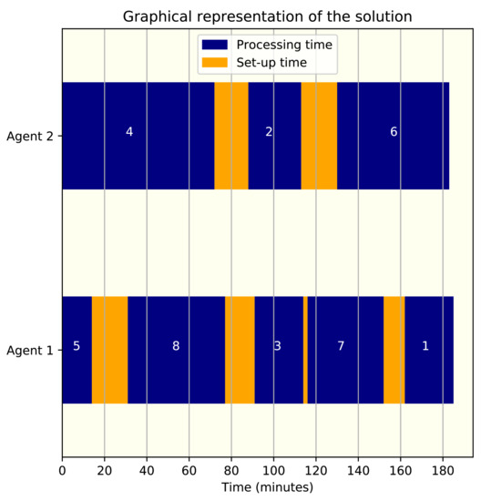
Figure A1.
Graphical solution of the instance used for the exemplification of the heuristics.
Appendix C. Examples of the Model Application
All of the data presented in this section is fictional and is only used to exemplify the applications of the model.
Appendix C.1. Scheduling of Automotive Seat Tests
When a person is sitting in a front car seat, either driving or in the passenger seat, unconsciously, she/he is continually making down-up movements, caused by the vibration generated by the transit of the car on surfaces that are never completely smooth. The movement of the person and the seat is shown in Figure A2.
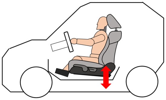
Figure A2.
Vibration in automotive seats.
The person in the seat has a weight, w, that is supported by the seat. The vibration combined with the weight of the passenger could cause severe affectations in the seat, such as aesthetic affectation, especially in the areas that are in contact with the person (gluteus cush and lumbar support), as well as structural and safety affectations, e.g., cracks in the metal structure behind the cloth and sponge of the seat. Before selling a new car model, automotive manufacturers must ensure that the vibration does not cause affectations in the seat, to do so, simulations are performed in specialized laboratories under controlled environments. The tests are prepared by engineers, who set up the seat in a jounce tester machine to simulate the vibration, as shown in Figure A3.
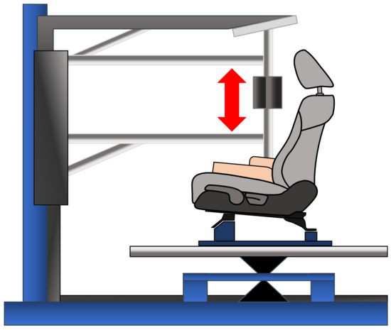
Figure A3.
Vibration simulation in automotive seats.
Let us suppose we are in charge of a seat test laboratory, where 8 employees work and 8 different jounce tester machines are available in parallel. We need to perform several vibrations tests for the seats of car models K10H, J21W and L21C from a French manufacturer, and to make the best use of the machine’s operating time and the engineers’ time, it is necessary to schedule the tests in such a way that the jobs take as little time as possible. The jobs to be scheduled and the engineers available are presented in Table A2.
Table A2.
Engineers and tests to be scheduled in jounce tester machines.
Table A2.
Engineers and tests to be scheduled in jounce tester machines.
| Engineer | ID | Test | ID |
|---|---|---|---|
| Sebastián | 1 | K10H FR LH MY 20 | 1 |
| Alejandro | 2 | K10H FR RH MY 20 | 2 |
| Refugio | 3 | K10H FR LH MY 21 | 3 |
| Gustavo | 4 | K10H FR RH MY 21 | 4 |
| Nazareth | 5 | K10H FR LH MY 22 | 5 |
| Silvia | 6 | K10H FR RH MY 22 | 6 |
| Iván | 7 | J21W FR LH MY 20 | 7 |
| Adán | 8 | J21W FR RH MY 20 | 8 |
| J21W FR LH MY 21 | 9 | ||
| CODES | J21W FR RH MY 21 | 10 | |
| FR: Front | J21W FR LH MY 22 | 11 | |
| LH: Left hand side | J21W FR RH MY 22 | 12 | |
| RH: Right hand side | L21C FR LH MY 21 | 13 | |
| MY: Model year | L21C FR RH MY 21 | 14 | |
| L21C FR RH MY 22 | 15 |
This problem represents an instance of 8 agents and 15 jobs. After solving the instance with the models proposed (and obtaining an optimal maximum makespan of 260), we can inform their schedule to the employees (optimal assignation of machines and jobs), as presented in Table A3.
Table A3.
Engineers schedule for vibration tests.
Table A3.
Engineers schedule for vibration tests.
| Person | Jounce Tester | Test (in That Order) |
|---|---|---|
| Sebastián | 1 | 3 |
| Alejandro | 8 | 4-11 |
| Refugio | 7 | 13-14 |
| Gustavo | 6 | 6-8 |
| Nazareth | 2 | 5-9 |
| Silvia | 3 | 2-1 |
| Iván | 4 | 12-15 |
| Adán | 5 | 10-7 |
From the solution, we can also obtain the time in which each job will be finished, as presented in Table A4. Figure A4 shows the graph representation of the engineer’s schedule.
Table A4.
Finalization time for vibration tests.
Table A4.
Finalization time for vibration tests.
| Test | Finished at Time (Minutes) |
|---|---|
| 1 | 256 |
| 2 | 73 |
| 3 | 150 |
| 4 | 103 |
| 5 | 97 |
| 6 | 50 |
| 7 | 241 |
| 8 | 184 |
| 9 | 244 |
| 10 | 94 |
| 11 | 253 |
| 12 | 52 |
| 13 | 130 |
| 14 | 260 |
| 15 | 240 |
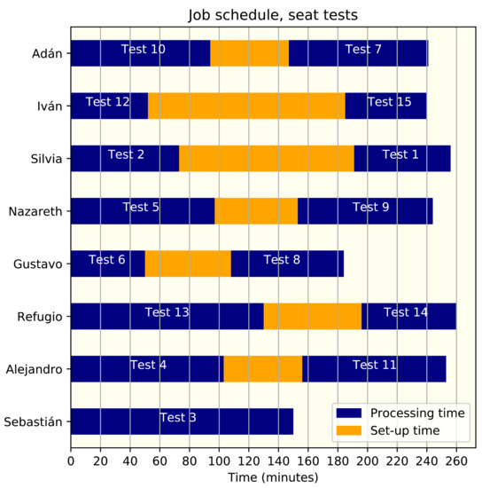
Figure A4.
Vibration tests schedule for the engineers.
Appendix C.2. Hemodialysis Scheduling in Hospitals
When a person’s kidneys are not healthy, they suffer from so-called renal failure: toxic wastes from the blood are not filtered, hydration is not regulated, urine is not produced properly, and the concentration of substances in the blood cannot be regulated. Renal failure can be treated with hemodialysis, a purification process that helps to filter water and toxins from the blood. To perform the hemodialysis, a nurse prepares the process of placing needles in the patient’s arm. The artificial kidney is then programmed by the nurse and makes it operate the time the patient needs, the machine pumps blood through a filter and back into the body. When the artificial kidney is operating, a nurse must monitor the process at all moments, to safeguard the patient’s condition [47].
Let us suppose we are the nurse in chief of the hemodialysis zone in a hospital. There are 3 nurses on a 14-h shift and 3 different parallel artificial kidneys in the area, and for the next day, 10 patients must receive their treatment. It is needed to schedule the treatments in such a way that all the hemodialysis are finished in the shorter possible time, to make the best use of the artificial kidneys’ operating time, to increase the utilization percentage of the nurses, and to indicate the patients the exact time they have to show up in the hospital, to do not make them wait until the beginning of their treatment. Based on the hospital rules, the patients must be in the hospital 10 min before their appointment, and the hemodialysis process and work shift start at 8 a.m. The hemodialysis to be scheduled and the nurses available are shown in Table A5.
Table A5.
Nurses and hemodialysis to be scheduled in artificial kidneys.
Table A5.
Nurses and hemodialysis to be scheduled in artificial kidneys.
| Nurse | ID | Hemodialysis | ID |
|---|---|---|---|
| Marisol | 1 | Female, 30 years old | 1 |
| Josué | 2 | Female, 58 years old | 2 |
| Tania | 3 | Male, 45 years old | 3 |
| Male, 59 years old | 4 | ||
| Female, 53 years old | 5 | ||
| Male, 81 years old | 6 | ||
| Female, 41 years old | 7 | ||
| Female, 70 years old | 8 | ||
| Male, 39 years old | 9 | ||
| Female, 65 years old | 10 |
The problem represents an instance of 3 agents and 10 jobs. After solving the instance, an optimal maximum makespan of 756 is obtained. With the solution, we can inform the nurses of their schedule for the next day, as presented in Table A6.
Table A6.
Nurses schedule for hemodialysis.
Table A6.
Nurses schedule for hemodialysis.
| Person | Artificial Kidney | Hemodialysis (in That Order) |
|---|---|---|
| Marisol | 2 | 7-1-4-10 |
| Josué | 3 | 9-2-5 |
| Tania | 1 | 3-6-8 |
From the solution, the time in minutes that each hemodialysis will finish was also obtained, as presented in Table A7. The time that each patient is notified to show up is shown (remember that the treatments start at 8:00 a.m. and the patient must be in the hospital 10 min before her/his appointment, before the set-up time corresponding to the treatment).
Table A7.
Appointments and finalization time for hemodialysis.
Table A7.
Appointments and finalization time for hemodialysis.
| Patient/ Hemodialysis | Appointment (Hour of the Day) | Finished at (Hour of the Day) | Finished at Time (Minutes after 8:00 a.m.) |
|---|---|---|---|
| 1 | 08:34 | 13:11 | 321 |
| 2 | 11:35 | 15:45 | 475 |
| 3 | 07:50 | 11:36 | 226 |
| 4 | 13:01 | 16:54 | 544 |
| 5 | 15:35 | 19:30 | 700 |
| 6 | 11:26 | 16:14 | 504 |
| 7 | 07:50 | 08:44 | 54 |
| 8 | 16:04 | 19:35 | 705 |
| 9 | 07:50 | 11:45 | 235 |
| 10 | 16:44 | 20:26 | 756 |
Figure A5 shows the graphical representation of the scheduling of hemodialysis.
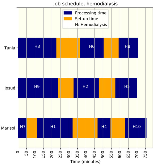
Figure A5.
Hemodialisys schedule for the nurses.
References
- Dhayanithi, A.; Deepak, S. Cost Optimization in Production Systems. Ph.D. Thesis, Jönköping University, Jönköping, Sweden, 2019. [Google Scholar]
- Zhao, K.; Lu, X.; Gu, M. A new approximation algorithm for multi-agent scheduling to minimize makespan on two machines. J. Sched. 2016, 19, 21–31. [Google Scholar] [CrossRef]
- Mokotoff, E. Parallel machine scheduling problems: A survey. Asia-Pac. J. Oper. Res. 2001, 18, 193. [Google Scholar]
- Abedinnia, H.; Glock, C.H.; Schneider, M.D. Machine scheduling in production: A content analysis. Appl. Math. Model. 2017, 50, 279–299. [Google Scholar] [CrossRef]
- Fan, K.; Zhai, Y.; Li, X.; Wang, M. Review and classification of hybrid shop scheduling. Prod. Eng. 2018, 12, 597–609. [Google Scholar] [CrossRef]
- Azzouz, A.; Ennigrou, M.; Said, L.B. Scheduling problems under learning effects: Classification and cartography. Int. J. Prod. Res. 2018, 56, 1642–1661. [Google Scholar] [CrossRef] [Green Version]
- Fuchigami, H.Y.; Rangel, S. A survey of case studies in production scheduling: Analysis and perspectives. J. Comput. Sci. 2018, 25, 425–436. [Google Scholar] [CrossRef] [Green Version]
- Abedinnia, H.; Glock, C.H.; Grosse, E.H.; Schneider, M. Machine scheduling problems in production: A tertiary study. Comput. Ind. Eng. 2017, 111, 403–416. [Google Scholar] [CrossRef]
- Mohan, J.; Lanka, K.; Rao, A.N. A Review of Dynamic Job Shop Scheduling Techniques. Procedia Manuf. 2019, 30, 34–39. [Google Scholar] [CrossRef]
- Allahverdi, A. The third comprehensive survey on scheduling problems with setup times/costs. Eur. J. Oper. Res. 2015, 246, 345–378. [Google Scholar] [CrossRef]
- Vallada, E.; Ruiz, R. A genetic algorithm for the unrelated parallel machine scheduling problem with sequence dependent setup times. Eur. J. Oper. Res. 2011, 211, 612–622. [Google Scholar] [CrossRef] [Green Version]
- Tran, T.T.; Araujo, A.; Beck, J.C. Decomposition methods for the parallel machine scheduling problem with setups. INFORMS J. Comput. 2016, 28, 83–95. [Google Scholar] [CrossRef] [Green Version]
- Fanjul-Peyro, L.; Ruiz, R.; Perea, F. Reformulations and an exact algorithm for unrelated parallel machine scheduling problems with setup times. Comput. Oper. Res. 2019, 101, 173–182. [Google Scholar] [CrossRef]
- Wang, L.; Wang, S.; Zheng, X. A hybrid estimation of distribution algorithm for unrelated parallel machine scheduling with sequence-dependent setup times. IEEE/CAA J. Autom. Sin. 2016, 3, 235–246. [Google Scholar] [CrossRef]
- Abreu, L.R.; Prata, B.A. A hybrid genetic algorithm for solving the unrelated parallel machine scheduling problem with sequence dependent setup times. IEEE Lat. Am. Trans. 2018, 16, 1715–1722. [Google Scholar] [CrossRef]
- Gedik, R.; Kalathia, D.; Egilmez, G.; Kirac, E. A constraint programming approach for solving unrelated parallel machine scheduling problem. Comput. Ind. Eng. 2018, 121, 139–149. [Google Scholar] [CrossRef]
- Ezugwu, A.E.; Adeleke, O.J.; Viriri, S. Symbiotic organisms search algorithm for the unrelated parallel machines scheduling with sequence-dependent setup times. PLoS ONE 2018, 13, e0200030. [Google Scholar] [CrossRef]
- Jouhari, H.; Lei, D.; Al-qaness, M.A.; Elaziz, M.A.; Ewees, A.A.; Farouk, O. Sine-cosine algorithm to enhance simulated annealing for unrelated parallel machine scheduling with setup times. Mathematics 2019, 7, 1120. [Google Scholar] [CrossRef] [Green Version]
- Santos, H.G.; Toffolo, T.A.; Silva, C.L.; Vanden Berghe, G. Analysis of stochastic local search methods for the unrelated parallel machine scheduling problem. Int. Trans. Oper. Res. 2019, 26, 707–724. [Google Scholar] [CrossRef]
- Marti, R.; Marcos Moreno-Vega, J. MultiStart Methods. Intel. Artif. 2003, 7, 355–368. [Google Scholar] [CrossRef]
- Schulze, M.; Rieck, J.; Seifi, C.; Zimmermann, J. Machine scheduling in underground mining: An application in the potash industry. OR Spectr. 2016, 38, 365–403. [Google Scholar] [CrossRef]
- Mao, J.y.; Pan, Q.k.; Miao, Z.h.; Gao, L. An effective multi-start iterated greedy algorithm to minimize makespan for the distributed permutation flowshop scheduling problem with preventive maintenance. Expert Syst. Appl. 2021, 169, 114495. [Google Scholar] [CrossRef]
- Avalos-Rosales, O.; Angel-Bello, F.; Alvarez, A. Efficient metaheuristic algorithm and re-formulations for the unrelated parallel machine scheduling problem with sequence and machine-dependent setup times. Int. J. Adv. Manuf. Technol. 2015, 76, 1705–1718. [Google Scholar] [CrossRef]
- Afzalirad, M.; Rezaeian, J. Resource-constrained unrelated parallel machine scheduling problem with sequence dependent setup times, precedence constraints and machine eligibility restrictions. Comput. Ind. Eng. 2016, 98, 40–52. [Google Scholar] [CrossRef]
- Fanjul-Peyro, L.; Perea, F.; Ruiz, R. Models and matheuristics for the unrelated parallel machine scheduling problem with additional resources. Eur. J. Oper. Res. 2017, 260, 482–493. [Google Scholar] [CrossRef]
- Avalos-Rosales, O.; Angel-Bello, F.; Álvarez, A.; Cardona-Valdés, Y. Including preventive maintenance activities in an unrelated parallel machine environment with dependent setup times. Comput. Ind. Eng. 2018, 123, 364–377. [Google Scholar] [CrossRef]
- Afzalirad, M.; Shafipour, M. Design of an efficient genetic algorithm for resource-constrained unrelated parallel machine scheduling problem with machine eligibility restrictions. J. Intell. Manuf. 2018, 29, 423–437. [Google Scholar] [CrossRef]
- Cota, L.P.; Coelho, V.N.; Guimarães, F.G.; Souza, M.J. Bi-criteria formulation for green scheduling with unrelated parallel machines with sequence-dependent setup times. Int. Trans. Oper. Res. 2021, 28, 996–1017. [Google Scholar] [CrossRef]
- Bitar, A.; Dauzère-Pérès, S.; Yugma, C. Unrelated parallel machine scheduling with new criteria: Complexity and models. Comput. Oper. Res. 2021, 132, 105291. [Google Scholar] [CrossRef]
- Lee, W.C.; Wang, J.Y. A three-agent scheduling problem for minimizing the makespan on a single machine. Comput. Ind. Eng. 2017, 106, 147–160. [Google Scholar] [CrossRef]
- Lee, W.C.; Chung, Y.H.; Wang, J.Y. A parallel-machine scheduling problem with two competing agents. Eng. Optim. 2017, 49, 962–975. [Google Scholar] [CrossRef]
- Yu, F.; Wen, P.; Yi, S. A multi-agent scheduling problem for two identical parallel machines to minimize total tardiness time and makespan. Adv. Mech. Eng. 2018, 10, 1–14. [Google Scholar] [CrossRef] [Green Version]
- Peng, T.; Zhou, B. Scheduling multiple servers to facilitate just-in-time part-supply in automobile assembly lines. Assem. Autom. 2018, 38, 347–360. [Google Scholar] [CrossRef]
- Gu, M.; Gu, J.; Lu, X. An algorithm for multi-agent scheduling to minimize the makespan on m parallel machines. J. Sched. 2018, 21, 483–492. [Google Scholar] [CrossRef]
- Chen, R.X.; Li, S.S.; Li, W.J. Multi-agent scheduling in a no-wait flow shop system to maximize the weighted number of just-in-time jobs. Eng. Optim. 2019, 51, 217–230. [Google Scholar] [CrossRef]
- Cheng, T.C.; Kravchenko, S.A.; Lin, B.M. Server scheduling on parallel dedicated machines with fixed job sequences. Nav. Res. Logist. 2019, 66, 321–332. [Google Scholar] [CrossRef]
- Wang, D.; Yu, Y.; Yin, Y.; Cheng, T.C.E. Multi-agent scheduling problems under multitasking. Int. J. Prod. Res. 2020, 59, 3633–3663. [Google Scholar] [CrossRef]
- Alaei, M.R.K.; Soysal, M.; Elmi, A.; Banaitis, A.; Banaitiene, N.; Rostamzadeh, R.; Javanmard, S. A bender’s algorithm of decomposition used for the parallel machine problem of robotic cell. Mathematics 2021, 9, 1730. [Google Scholar] [CrossRef]
- Kim, H.J.; Lee, J.H. Scheduling uniform parallel dedicated machines with job splitting, sequence-dependent setup times, and multiple servers. Comput. Oper. Res. 2021, 126, 105115. [Google Scholar] [CrossRef]
- Cook, S.A. The Complexity of Theorem-Proving Procedures. In Proceedings of the Third Annual ACM Symposium on Theory of Computing, Shaker Heights, OH, USA, 3–5 May 1971; pp. 151–158. [Google Scholar]
- Karp, R.M. Reducibility among combinatorial problems. In Complexity of Computer Computations; Springer: Boston, MA, USA, 1972; pp. 85–103. [Google Scholar]
- Helal, M.; Rabadi, G.; Al-Salem, A. A tabu search algorithm to minimize the makespan for the unrelated parallel machines scheduling problem with setup times. Int. J. Oper. Res. 2006, 3, 182–192. [Google Scholar]
- Rabadi, G.; Moraga, R.J.; Al-Salem, A. Heuristics for the unrelated parallel machine scheduling problem with setup times. J. Intell. Manuf. 2006, 17, 85–97. [Google Scholar] [CrossRef]
- Logendran, R.; McDonell, B.; Smucker, B. Scheduling unrelated parallel machines with sequence-dependent setups. Comput. Oper. Res. 2007, 34, 3420–3438. [Google Scholar] [CrossRef]
- Fleszar, K.; Charalambous, C.; Hindi, K.S. A variable neighborhood descent heuristic for the problem of makespan minimisation on unrelated parallel machines with setup times. J. Intell. Manuf. 2012, 23, 1949–1958. [Google Scholar] [CrossRef]
- Glover, F. Tabu Search—Part I and Part II. J. Comput. 1989, 2, 4–32. [Google Scholar]
- Levy, J.; Brown, E.; Daley, C.; Lawrence, A. Oxford Handbook of Dialysis; Oxford University Press: Oxford, UK, 2010. [Google Scholar] [CrossRef]
Publisher’s Note: MDPI stays neutral with regard to jurisdictional claims in published maps and institutional affiliations. |
© 2021 by the authors. Licensee MDPI, Basel, Switzerland. This article is an open access article distributed under the terms and conditions of the Creative Commons Attribution (CC BY) license (https://creativecommons.org/licenses/by/4.0/).