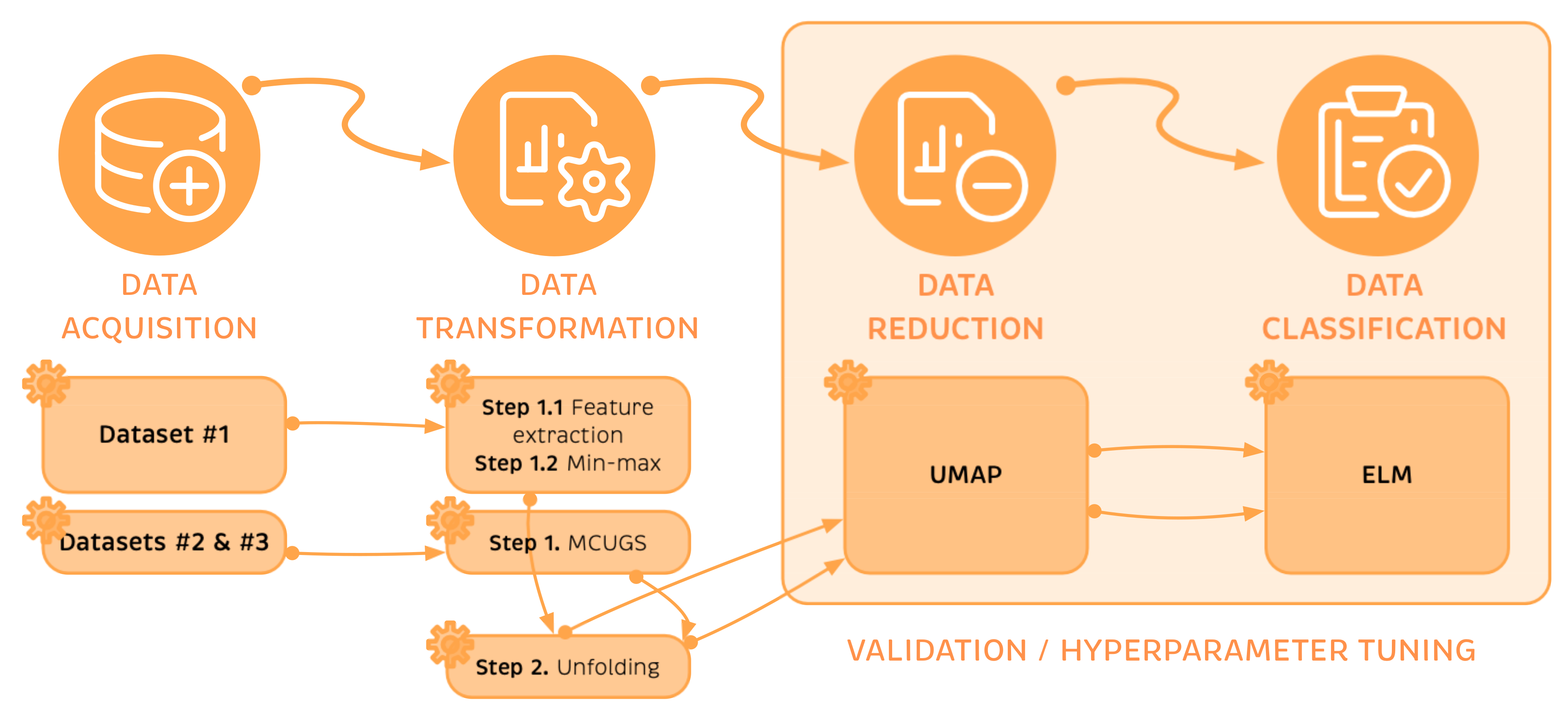
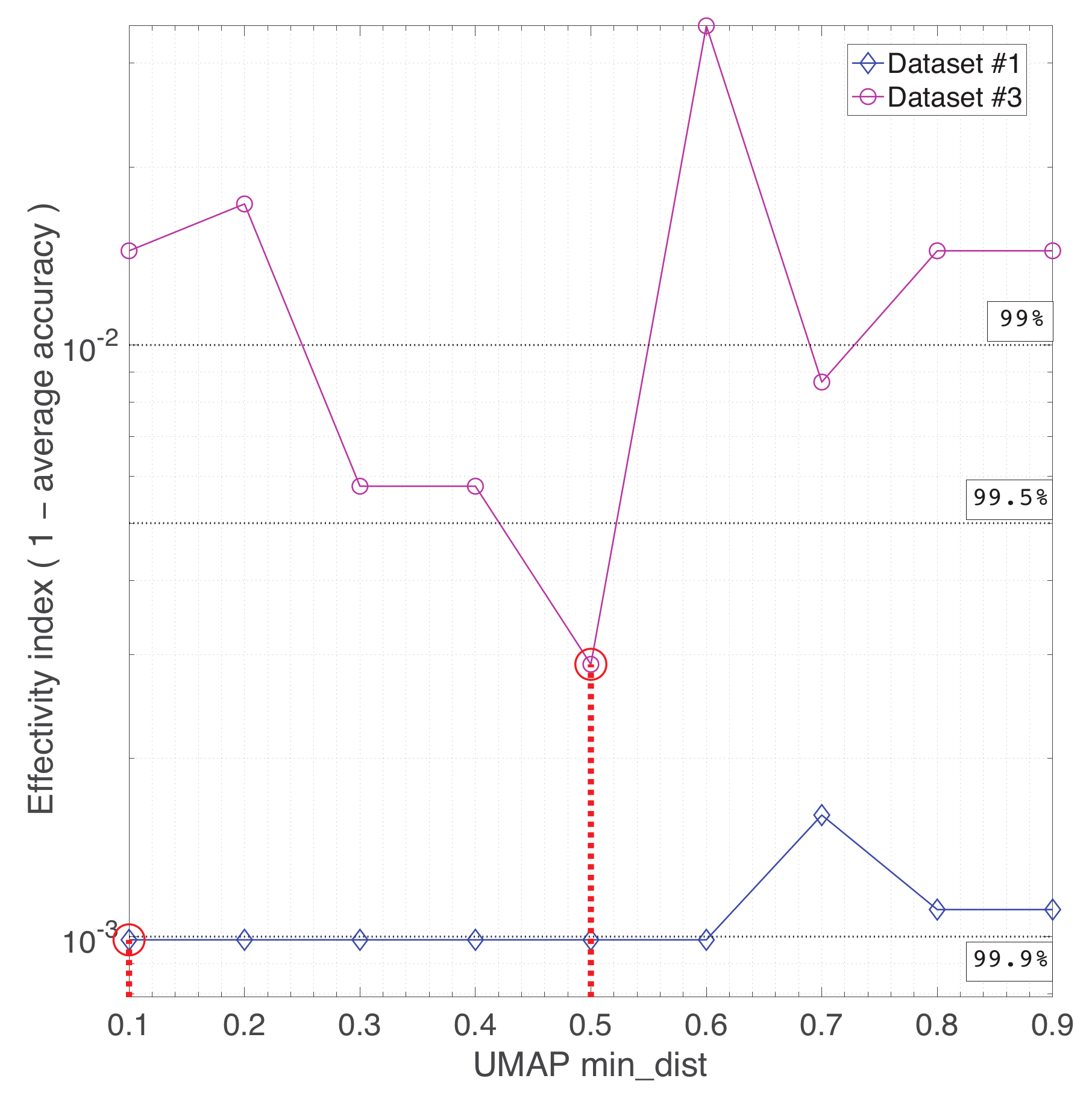
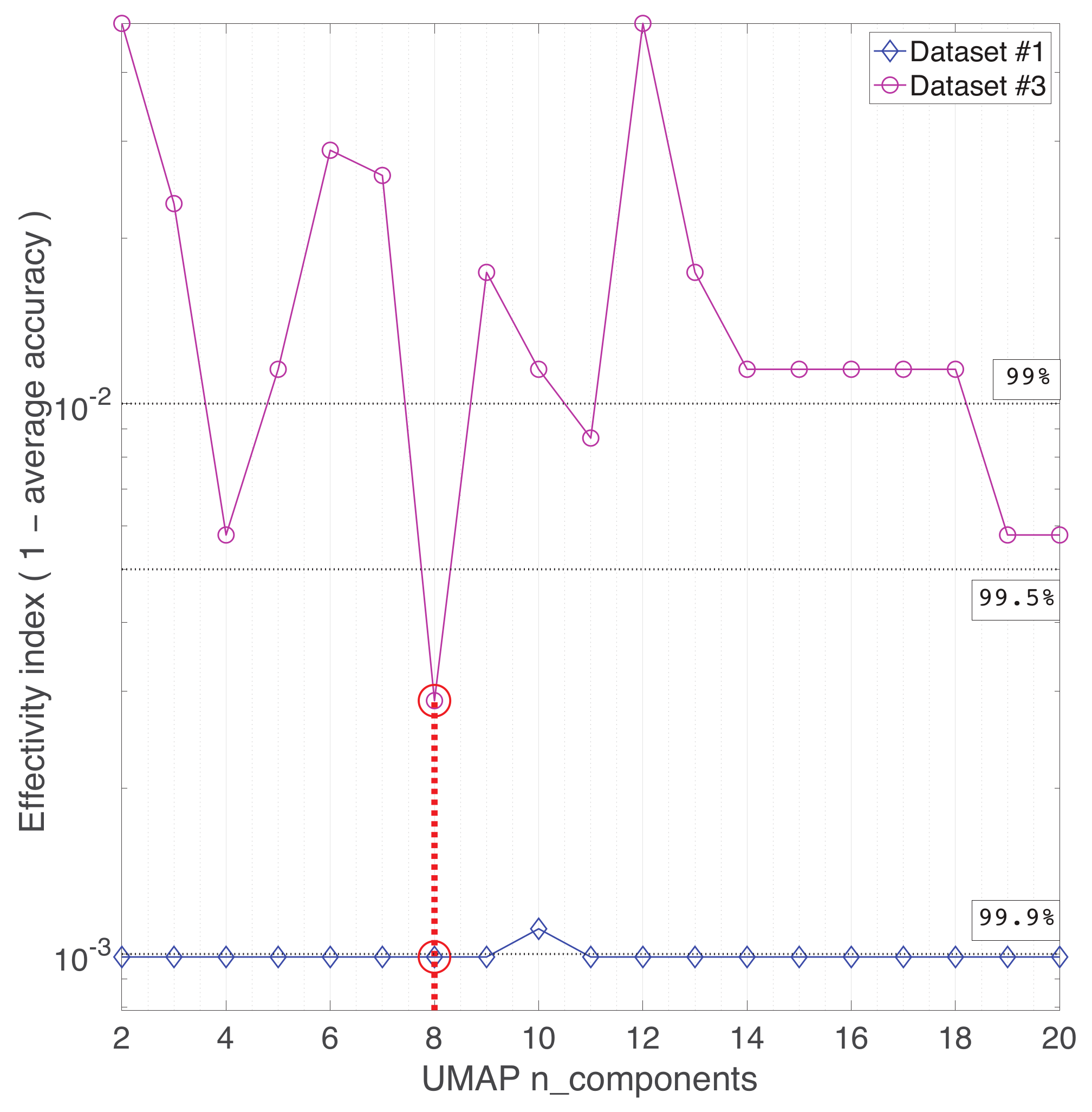
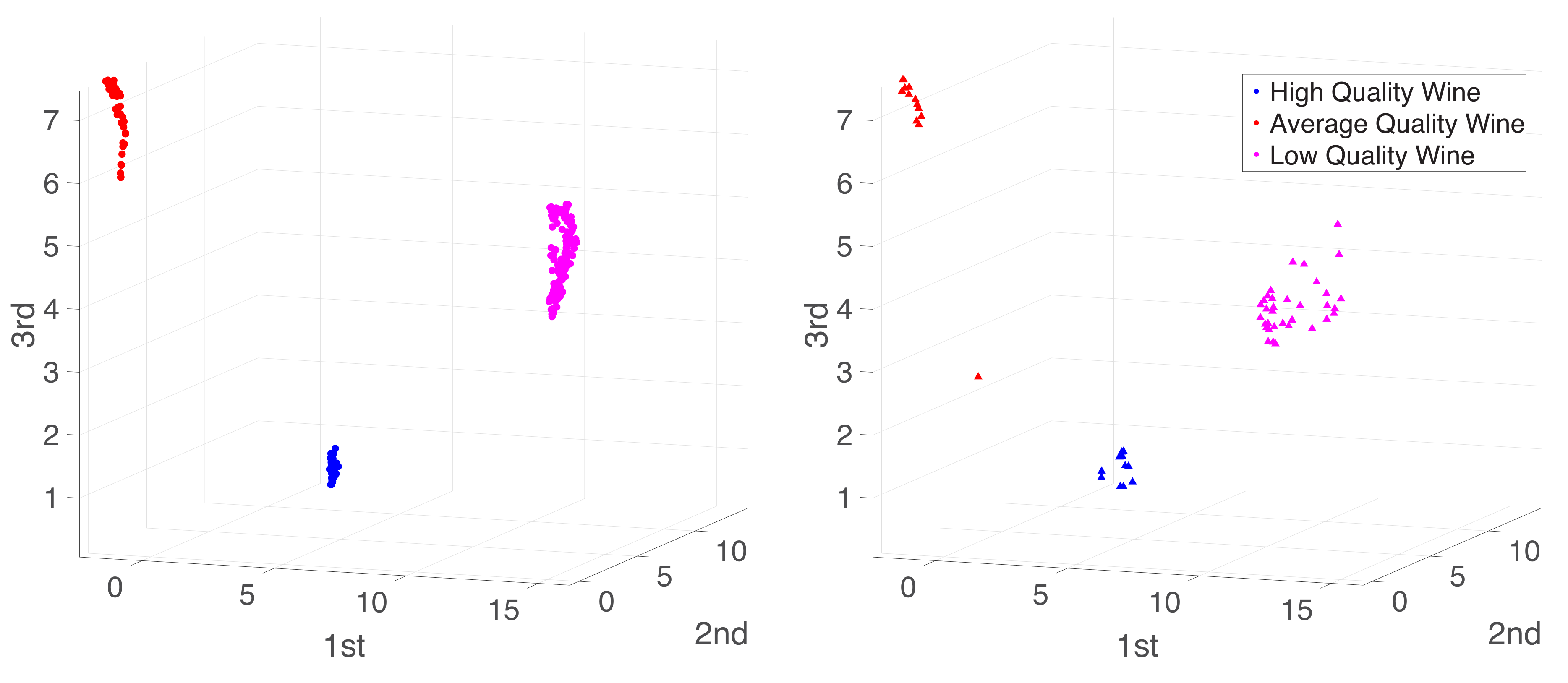
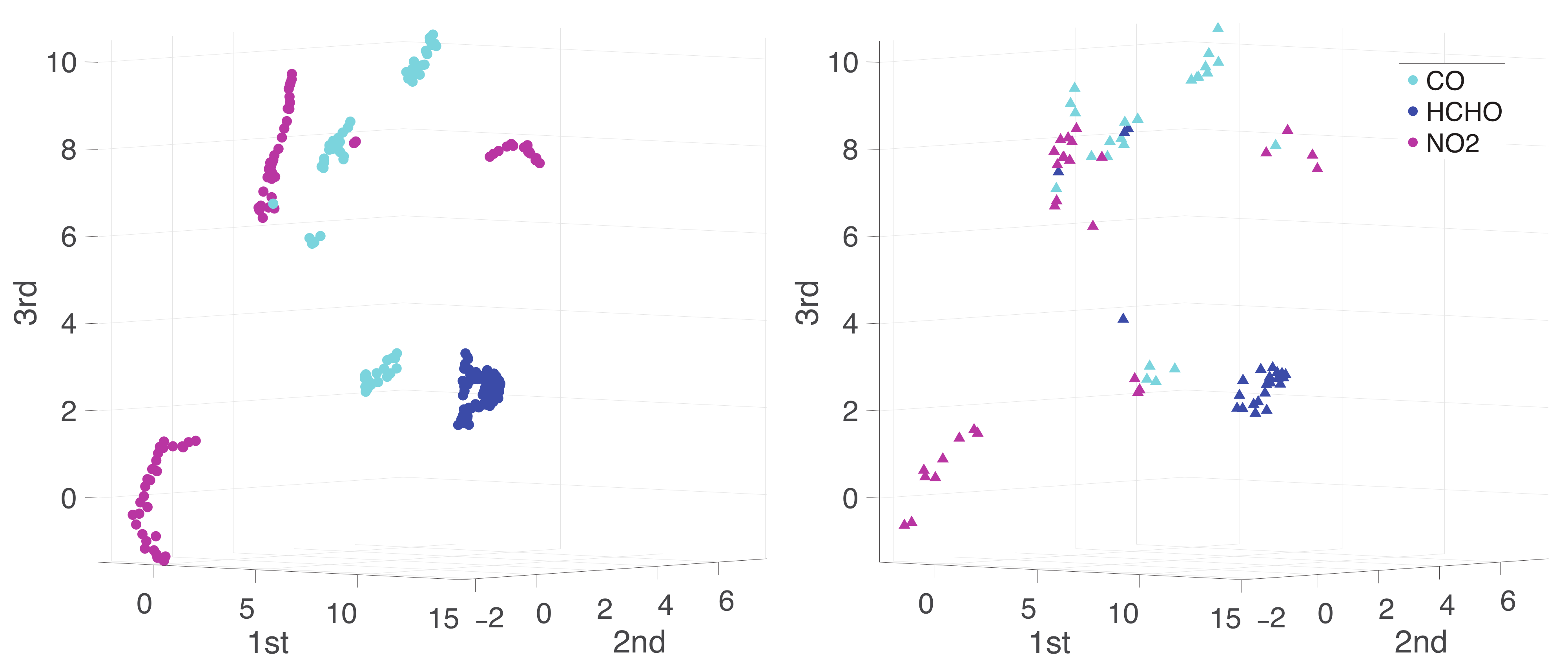
Appendix A. Practical Computational Description of the UMAP Method
This section presents a practical computational description of the UMAP method in terms of weighted graphs. Let
be a matrix collecting all the samples for a specific dataset, where
n denotes the total number of samples and
D denotes the total number of features describing the data. The aim is to determine a reduced low-order
d-dimensional manifold,
, described by the transformed matrix,
, that retains most of the information of the original matrix,
. In particular, in the present study, the aim is to obtain a transformed matrix,
, that provides an accurate classifier when used as an input of the machine learning algorithm. The UMAP transformed matrix,
, is computed in two phases. In the first phase, namely, graph construction, a weighted
k-neighbor graph is constructed, and after proper transformations are applied on the edges of the graph, the data,
, are represented by the adjacency matrix of this graph. Then, a low-dimensional representation of the previous graph preserving the desired characteristics of the graph, i.e., a graph layout, is built. Specifically, let
be the input data set:
where
; in addition, consider the metric
.
To fix these ideas, let
be the Euclidean distance, which is defined as:
where
denotes the
lst element entry of vector
, which coincides with
, i.e., the
th entry of matrix
. Then, given an input hyperparameter,
k, for each point
,
, we compute the set
of the
k-nearest neighbors of
under the metric
and define the parameters
and
such that:
and
(see
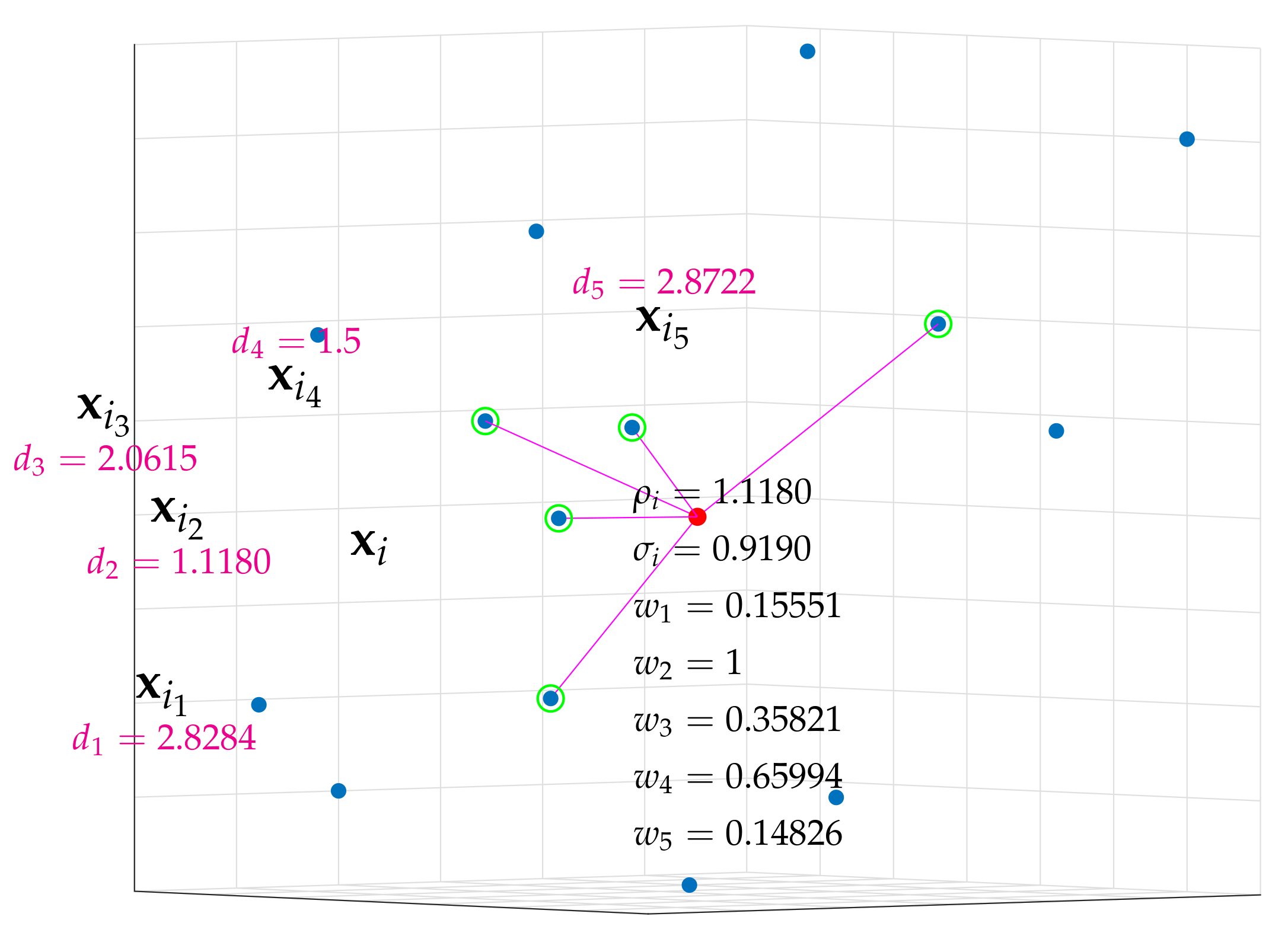
Figure A1). Note that
is the distance between point
and its nearest neighbor, whereas
is a smoothed normalization factor.
Figure A1.
Five nearest neighbors of point for a particular set of points in , where, for simplicity, and . The metric is the Euclidean distance.
Figure A1.
Five nearest neighbors of point for a particular set of points in , where, for simplicity, and . The metric is the Euclidean distance.
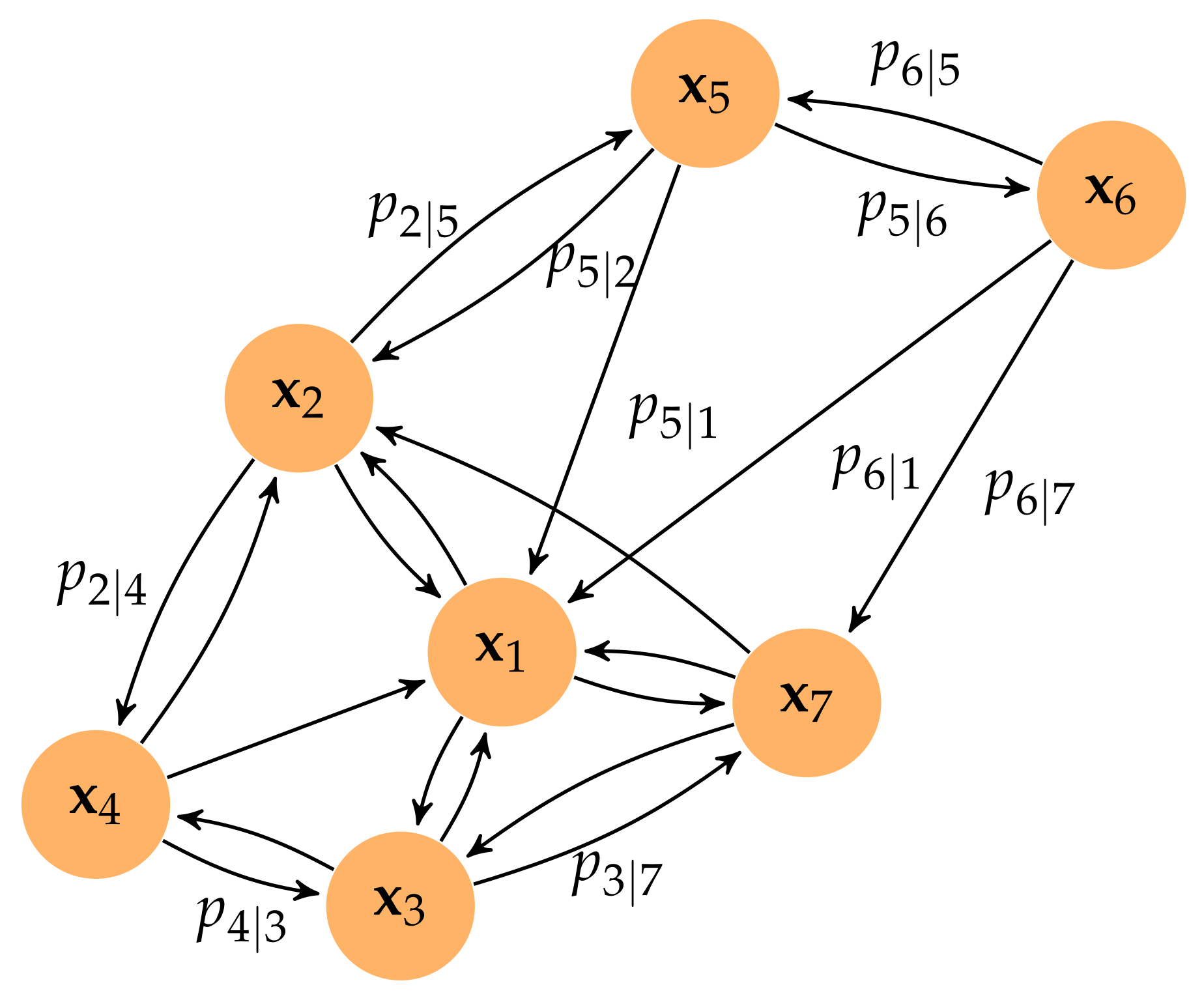
Then, the weighted directed
k-neighbor graph is defined as
, where vertices
V are the points
and the set of directed edges is
with the corresponding directed weights,
(see
Figure A2). It is worth noting that the definitions of
and
ensure that
, at least one edge has a weight of 1, non-existent edges are set to have a weight of 0, and all weights associated with the outcoming edges of every node sum to
. Weight
associated with the edge joining
and
represents the similarity between the high-dimensional points
and
, measured using an exponential probability distribution, which can also be seen as the probability that an edge joining
and
exists.
Figure A2.
Weighted directed three-neighbor graph for a particular set of points in . For clarity, only some weights are shown. The metric is the Euclidean distance.
Figure A2.
Weighted directed three-neighbor graph for a particular set of points in . For clarity, only some weights are shown. The metric is the Euclidean distance.
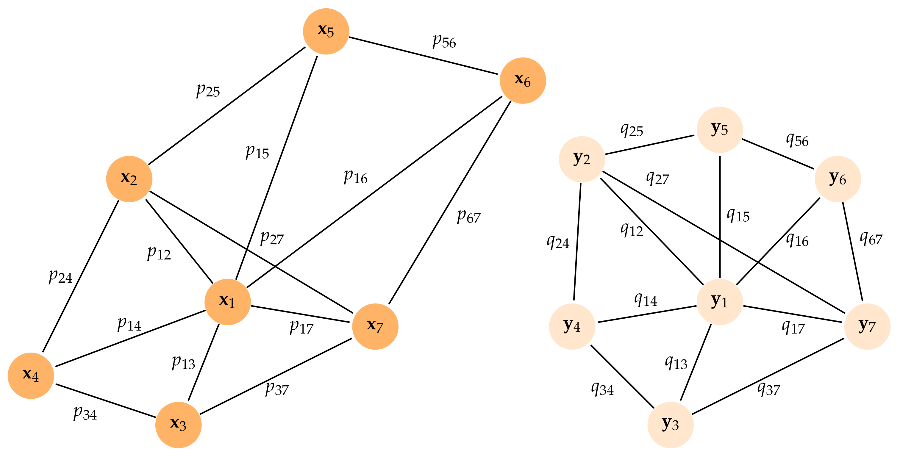
The last step of the graph construction phase is to recover an undirected graph from
G. The weights associated with the new undirected edges
are given by the triangular conorm or the probabilistic sum of the directed weights, namely,
which can be interpreted as the probability that at least one of the two directed edges (from
to
and from
to
) exists. The adjacency matrix of this undirected graph
containing the weights
in its corresponding
th position is the starting point of the UMAP procedure. Note that if
is the adjacency matrix of graph
G, then from Equation (
A2),
where ‘∘’ is the Hadamard (or pointwise) matrix product. It is worth noting that, in the initial step, the data matrix,
, is associated with a larger, although sparse,
matrix, where the new entries are probability-like measures of the distances between samples.
The aim of the second phase of the UMAP procedure is to compute a low-dimensional representation of the undirected graph preserving the main desired characteristics. That is, the goal is to compute a new transformed matrix,
:
where
, containing only
d features and a new undirected graph with associated weights defined by matrix
, which minimizes the cross-entropy between the two graphs, and is defined as follows:
where
and
are the weights of the undirected graphs given by the
th entries of the adjacency matrices
and
, (see
Figure A3). Since
for
, the goal of UMAP is to try to find a low-dimensional representation of the data trying to mimic the similarities
in a high-dimensional space.
Figure A3.
Illustration of a weighted undirected graph for points in and a low-order representation of the graph where . The weights in the original space are computed from distances measured in the -metric of the k-neighbors of each point, whereas the weights are computed from pairwise Euclidean distances.
Note that the values of
, which are computed from
, are fixed and that the weights
are computed from the
d features of the samples stored in
. Therefore, after the constant terms in the objective function are removed, the problem at hand translates to finding
by minimizing:
To use the stochastic gradient descent (SGD) method in the previous optimization problem, we consider a smooth function describing the similarities between the pairs of points in the low-dimensional space
:
where
a and
b can be user-defined positive parameters or automatically set by solving a nonlinear least squares fitting, once the minimum distance between the points in the low-dimensional representation (
min_dist hyperparameter) and the effective scale of the embedded points (
spread hyperparameter) is fixed. Specifically,
a and
b are found, if not previously given, fitting the real function
to the exponential decay function:
for
. For instance, for the reference values
and
, we have
and
(see [
66] for details).
Therefore, after an initial guess
is computed, an iterative procedure is applied to find the minimum value in Equation (
A4). The initial guess for the SGD method is the largest eigenvectors of the symmetric normalized graph Laplacian associated with
(see [
67]). Specifically, we denote by
the degree matrix of the undirected graph
(
, where
), and by
the normalized graph Laplacian; then,
is the matrix containing only the first
d eigenvectors with the largest eigenvalues.
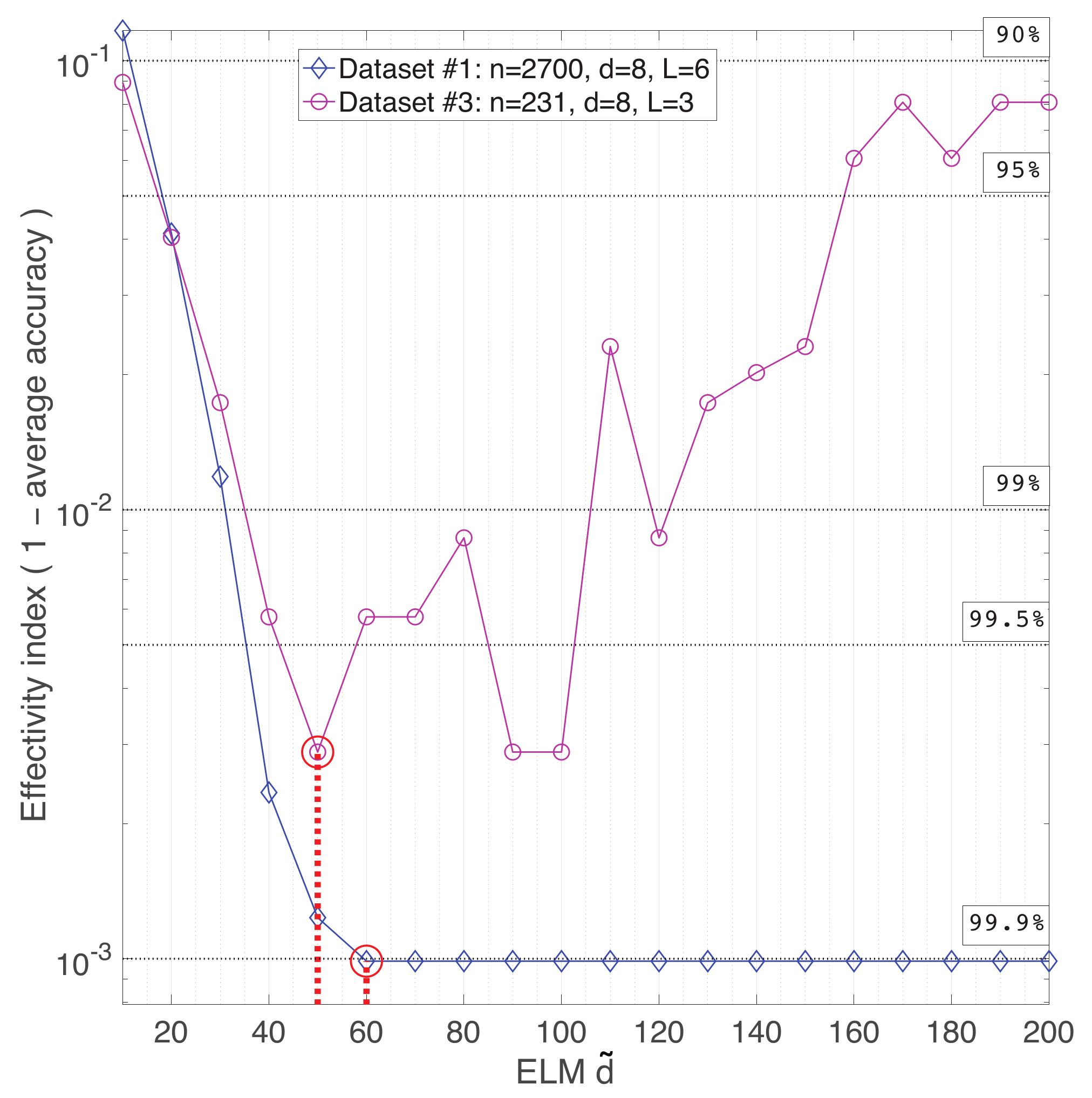
Appendix B. Practical Computational Description of Extreme Learning Machine
Let
be a matrix collecting the
n samples given in Equation (
A3) to be classified, where each specific sample is given by
and
d indicates the relevant features selected by the UMAP algorithm. In addition, let
be the classes/labels into which the samples must be classified, where
L denotes the total number of classes. The ELM classifier takes as input a particular sample,
, and returns the output vector,
, containing the raw score of the class membership to each of the
L classes. By default, the ELM method uses binarized
class labels, and thus, if sample
belongs to class
, we expect that
, i.e., we expect the
th component of the vector to be close to 1 and all the other components to be close to
. The class prediction is then computed by selecting the maximum component of
:
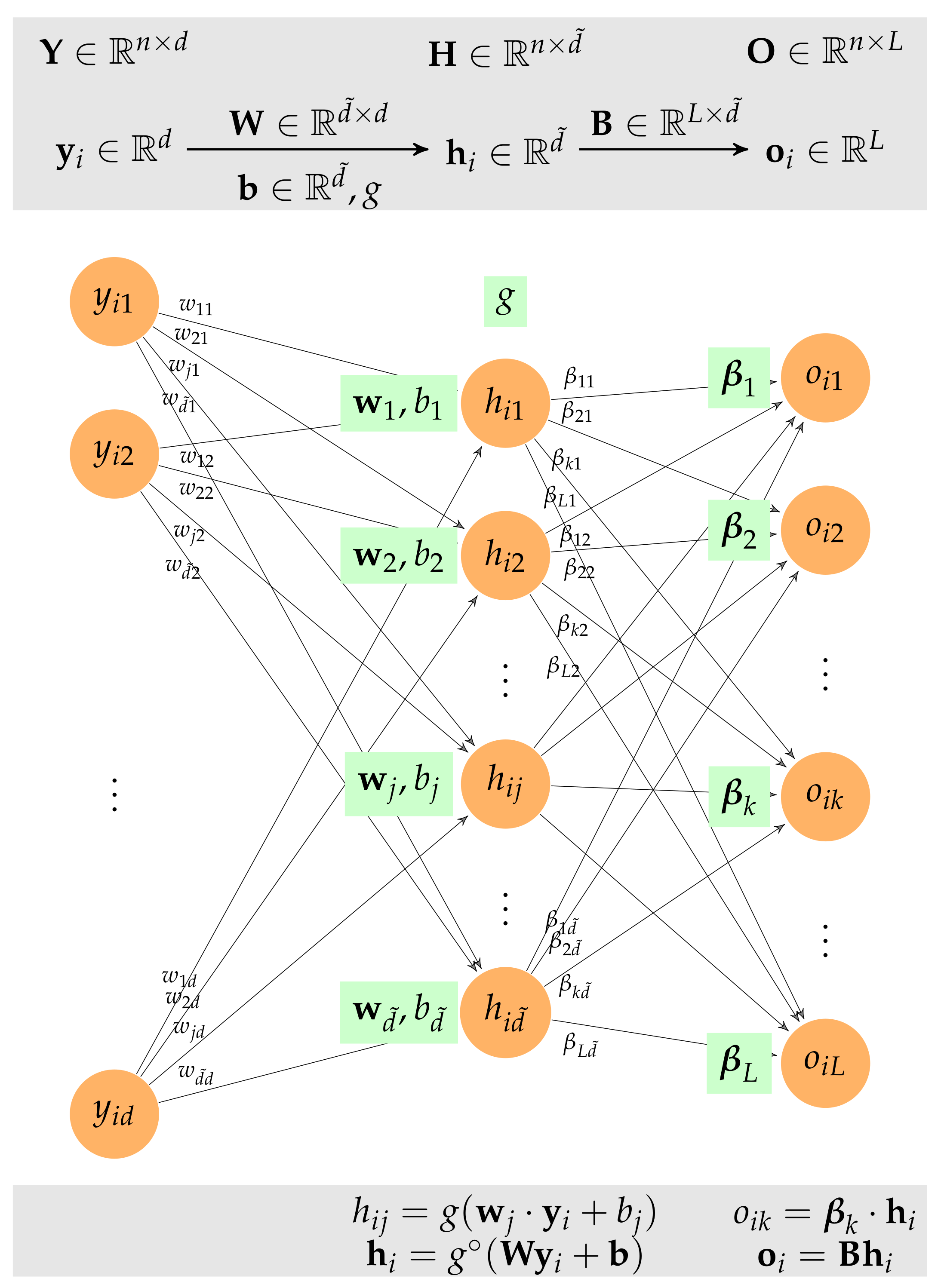
The output vector, , is computed from by introducing a hidden intermediate layer in the neural network represented by vector , where denotes the number of nodes in the hidden layer.
In general, every layer of a neural network that takes as input a feature vector, , and returns an output vector, , is characterized by:
- (1)
An activation function ;
- (2)
An threshold or biases , collected in vector ; and
- (3)
weighting vectors , collected in the weighting matrix .
Thus, the output vector is computed as follows:
where
is the element-wise activation function that applies the activation function,
g, to each component of the vector. Based on this definition, it is easy to recover the usual alternative expression for the
jth component of the output vector:
In particular, the ELM neural network consists of a hidden layer that converts the initial samples
into the hidden feature vector
and an output layer that converts the hidden vector
into the output vector
(see
Figure A4). The hidden layer consists of a weight matrix
, a bias vector
, and a user-defined activation function
g, whereas the output layer consists of a weight matrix
, a zero-bias vector, and an identity activation function. Therefore, after composing the two layers, we obtain an output vector of:
Once the neural network parameters are set, it is straightforward to provide the class prediction for any given sample.
As mentioned before, the training step of the ELM neural network is comparable to that of a traditional neural network, because the weights and biases of the hidden layer are randomly assigned at the beginning of the learning process and remain unchanged during the entire training process. In particular, once the hidden number of features
is set, the hidden weights and biases are randomly computed using the standardized normal distribution:
Figure A4.
The ELM neural network consists of a hidden layer that converts the initial samples into the hidden feature vector and an output layer that converts the hidden vector into the output vector .
Figure A4.
The ELM neural network consists of a hidden layer that converts the initial samples into the hidden feature vector and an output layer that converts the hidden vector into the output vector .
Therefore, only the weights of the output layer are computed using the training dataset. To illustrate the computation of , for ease of presentation and without loss of generality, let us assume that all data are used to train the neural network (in practice, only some of the total data are used for training the ELM classifier, and should be replaced by ).
Because the class of the training samples is known, the raw score of the class membership for each sample is stored in the true output matrix:
where
corresponds to the raw scores of the
ith sample (containing
in the non-actual class and 1 in the actual class). Specifically, if the
ith sample belongs to class
, then
if
and
otherwise. Moreover, because the hidden layer is already known and is described by
, we can compute all the hidden features of the input samples
and collect them in the matrix:
where the vectors
are now placed in the rows of matrix
. Then, the output of the ELM neural network is:
where recall that
.
The output weights are then computed by minimizing the distances between the true outputs
and the predictions
, namely, by finding a least-squares solution
of the linear system
:
where the Frobenius norm of a matrix is
. Note that the system of equations,
, represents the
restrictions to be met, matrix
has
degrees of freedom, and, in general, the ELM can only approximate the training samples with zero error if the number of hidden nodes coincides with the total number of samples,
, in which case,
. In the general case in which
(note that the number of hidden nodes is usually much smaller than the number of samples), the output weights are computed by solving the least-squares problem in Equation (
A8), yielding:
where
is the Moore-–Penrose generalized inverse of
(see [
68]). To further describe this key computation of the training step, despite the Moore–Penrose pseudo-inverse usually being computed using a singular decomposition of the matrix, in the usual case in which
, we have the following:
The training steps of the ELM are summarized in Algorithm A1.
Algorithm A1 shows that the hidden layer parameters are randomly generated, independently of the dataset, and that the weights associated with the output layer are the only parameters that need to be trained. Equation (
A9) reveals that the weights are computed explicitly without the use of an iterative procedure, and therefore, the ELM has a higher training speed than the BP learning algorithm.
| Algorithm A1. ELM neural network training for classification. |
Input: A training dataset, , of n samples containing d features; the class labels of the samples, ; the number of nodes in hidden layer, ;
the activation function, g, of the hidden layer. |
Output: ELM classifier- 1:
Create the true raw score class membership matrix, , using binarized class labels, where if or , otherwise. - 2:
Randomly generate weighting matrix and bias vector of the hidden layer, , where . - 3:
Compute the output matrix of the hidden layer, , associated with , namely, , where . - 4:
Compute the weights of the output layer, .
|


 ,
, 


