Response Times Reconstructor Based on Mathematical Expectation Quotient for a High Priority Task over RT-Linux

Abstract

Every computer task generates response times depending on the computer hardware and software. The response times of tasks executed in real-time operating systems such as RT-Linux can vary as their instances evolve even though they always execute the same algorithm. This variation decreases as the priority of the tasks increases; however, the minimum and maximum response times are still present in the same task, and this complicates its monitoring, decreasing its level of predictability in case of contingency or overload, as well as making resource sizing difficult. Therefore, the need arises to propose a model capable of reconstructing the dynamics of response times for the instances of a task with high priority in order to analyze their offline behavior under specific working conditions. For this purpose, we develop the necessary theory to build the response time reconstruction model. Then, to test the proposed model, we set up a workbench consisting of a single board computer, PREEMPT_RT, and a high priority task generated by the execution of a matrix inversion algorithm. This work demonstrates the application of the theory in an experimental process, presenting a way to model and reconstruct the dynamics of response times by a high-priority task on RT-Linux.

1. Introduction

One of the main performance issues on real-time computing systems is determining whether a set of tasks can be processed without exceeding their deadlines. For real-time systems (RTS), compliance with timing constraints imposed by the world is required. According to G. Buttazzo in [1], real-time systems are classified as critical (hard real-time) and non-critical (soft real-time). The end time $f_{i,k}$ (see

Table 1. List of variables.

Variable	Description
J	Tasks set
$J_i$	Task
$j_{i,k}$	Instance of a task
$l_{i,k}$	Arrival time
$o_{i,k}$	Operation time
$s_{i,k}$	Start time
$c_{i,k}$	Computing time
$p_{i,k}$	Preemption time
$f_{i,k}$	End time
$r_{i,k}$	Response time
$u_{i,k}$	System input
$v_{i,k}$	Internal noise
$w_{i,k}$	External noise
$e_{i,k}$	Reconstruction error
${\widehat{r}}_{i,k}$	Reconstructed response time
i	Task index
k	Instance index
n	Total number of tasks
m	Total number of instances
$\alpha$	Total number of segment times
a	System parameter
$\widehat{a}$	Estimated system parameter
$\mu e_{i,k}^2$	Mean squared error

) is a timing constraint that allows limiting the value when a task or process ends. In critical systems, we find that $f_{i,k}<d_{i,k}\forall i,k\in {\mathbb{Z}}^{+}$; while deadline $d_{i,k}$ depends on the real-world and its dynamic, calculated by sampling criteria such as the elemental theory proposed by Nyquist [2], Shannon, and Kotel’nikov [3], etc. The response time $r_{i,k}$ on a real-time operating system has a random behavior, as the fluctuation of the execution time can be due to computational factors: such as caching, pipeline, execution path finding, among others [4]. The run-time $c_{i,k}$ and response time $r_{i,k}$ depend on the computers, hardware and software. In the case of response times, $r_{i,k}$ is the time that the processor deals with serving a k-th instance of an i-th task considering preemptions, scheduler operation time, start time and end time. Through response times measurement, it is possible to generate a mathematical model that allows knowing its dynamic with statistic characterization using first and second probability moments [5].

Therefore, this work is relevant as, currently, the field of application of single board computers is vast enough, and computational processes require to be in sync and have timing correctness. The quality of correct responses depends directly on the operating system, which is why we work with RT-Linux. To obtain real-time features in the standard Linux, we have modified it using the PREEMPT_RT patch. Some previous papers, as follows, support the use of RT-Linux. The authors of [6] asseverate that the PREEMPT_RT patch has the goal of increasing predictability and reducing the latency of the kernel. Furthermore, they claimed that Linux cannot be considered a real-time system strictly, at least not for safety-critical scenarios. In [7], the authors show that the RT-patch is suitable for units that emphasize data processing, which rely heavily on IPC (Inter-Process Communication). Wang et al. in [8] show amazing experiments using Linux and RT-Linux and the results showed that kernel optimized by RT-Linux patch generated less delay than the kernel in multi-thread scheduling. In the study of D. González [9], two real-time patches performance Xenomai and PREEMPT_RT were tested and compared. For the analysis of measured times, the first and second probability moments were used, which showed the best performance with the PREEMPT_RT patch and had lower variances and reduced response time. All of these papers show some advantages of using RT-Linux vs. standard Linux and other real-time patches.

Hence, the response times of tasks executed on real-time operating systems such as RT-Linux may vary as their instances evolve, even though they always execute the same algorithm; this is due to various causes such as operation times, preemption times, measurement noise, jitter, scheduling, message passing, hardware and software interruptions, among others [4]. This variation decreases as the priority of the tasks increases; however, the minimum and maximum response times are still present in the same task and this complicates its monitoring, decreasing its level of predictability in the case of contingency or overload, and in addition, making the sizing of resources difficult. Thus, the need arises to propose a model capable of reconstructing the dynamics of the response times of the instances of a task with high priority in order to analyze its offline behavior under different working conditions.

The major contributions of this work demonstrate the importance of applying the theory in an experimental process, where we present a method of modeling the dynamic of response times of a high priority task over RT-Linux. These contributions are shown as follows.

• Development of a theory for response times dynamic.
• Development of a model for response times reconstruction of a high priority task over RT-Linux.
• Development of a parameter estimator for the proposed model based on the quotient of mathematical expectation.
• Experimental validation of the proposed model through a real task running with high priority over RT-Linux.

In general terms, it is possible to contextualize a model as the representation of a developed concept that simplifies a complex reality and allows us to understand the behavior of such reality, with the firm purpose of using it in favor of what is convenient according to its application. Currently, there are different types of models, for example, process diagrams, and maps, music scores, or for this specific case, expressions that with mathematical tools describe the behavior of a physical phenomenon seen as a system. All models seek the total correct approximation to the reality to be represented, and in particular, these models shall have the characteristic of being as simple as possible, allowing a diversification of understanding to allow maximum usability. An alternative to model systems is the use of instruments provided by probability and statistics where probabilistic and statistical models are conceived that allow us to observe, study, and analyze in descriptive graphs their bounded dynamics.

This work was carried out as follows: First we present an overview of the context about modeling the systems and their application in real-time systems with a brief theoretical description of the main characteristics that represent them. In the related work subsection, we created a brief survey to show the most relevant findings of response times modeling. Then, in the materials and methods section, we developed and exposed the needed theory about response times dynamics to support and allow the building of a model that correctly represents the approach of the theoretical response time dynamics’ behavior. Finally, the results and conclusions highlight our findings and the future work in this field of knowledge.

Related Work

Liu et al. [10] describe run-times of periodic tasks; these times are used to calculate the achievable processor utilization, and this concept was the basis of future investigations. Joseph and Pandya in [11] explain that response times of a real-time system $R{T}_i$ is the sum of the computational requirements for all inputs from higher levels occurring in an interval. Sjodin and Hansson in [12] presented an example of response-time analysis. Additionally, they showed an equation of response time by the sum of maximum blocking from lower priority processes, maximum jitter, worst time, computation time, tasks period and deadline. In this sense, Bril et al. [13] presented a simple recursive equation to determine the best-case response times of periodic tasks under fixed-priority preemptive scheduling and arbitrary phasing. The authors of [14] followed the same sense of previous papers; they presented a recurrence equation to calculate the best-case response times of a periodic task set with fixed priorities. The solution is based on the identification of the best-case phasing of a low priority task compared to the higher priority tasks. This phasing occurs when the low priority task is released so that it finishes simultaneously with the releases of all higher priority tasks when these have experienced their maximum release jitter. Thus far, the reviewed five references have something in common. The authors propose some type of theoretical response-times model. All of them are the basis of a response times model in different scenarios. In [15], the authors present a model to estimate the worst-case response time of sporadic tasks with fixed priorities upon a preemptive uni-processor. They identified three desirable properties: continuity, efficient computability and approximability. Other papers that started this idea are shown in [13,14,16,17,18,19]. Lu et al. in [20,21] present a statistical approach to response-time analysis of embedded real-time systems, and their work is based on the extreme value theory, Monte Carlo simulations and other statistical methods of obtaining a probabilistic estimate; one characteristic of this paper is their experimental results based on data analysis. In [22], the authors suggest a probabilistic worst-case response time estimation oriented to multi-core real-time systems. Their work involves data generation with sample classification and sample size equalization, and the estimation is based on an extreme value distribution model and a generalized Pareto distribution model fit method. The threshold detection and parameter estimation is also presented. Last but not least, Rivera and Bril in [23] presented and proved a novel exact best-case response time analysis for independent real-time periodic tasks with arbitrary deadlines scheduled using fixed-priority scheduling with preemption thresholds (FPTS). They presented a complete theoretical development and different scenarios to prove the model.

The most valuable aspect of our work is that the model we propose takes into consideration variables that are involved in response times such as start time, scheduler operation time, computing time, preemption time, and end time. Our model validation is supported through a task running with high priority over RT-Linux. We measure the response times generated by the execution of the task, which calculates matrix inversion [24]. Then, we analyze the response times by statistical analysis, and this could be considered as a metric to know if the proposed model fits according to its characteristics and behavior. The validation of our model is totally experimental, and we do not simulate any data.

Hence, the statistical characterization of the response times experimentally measured in a high priority task executed on RT-Linux is taken as a reference for the reconstruction of the model. Subsequently, with the analyzed data, a reconstructor based on a linear autoregressive and time-invariant model and a parameter estimation based on the mathematical expectation quotient is proposed. Finally, the reconstruction error is calculated with the difference between the measured and reconstructed response times, thus validating the effectiveness of the reconstructor, as explained in the next section.

2. Materials and Methods

The proposed response time model is created by means of an autoregressive-moving average model, a linear system with a time invariant parameter and first order. These considerations are based on experimental measurements of response times with a high priority task over PREEMPT_RT. The reconstructor algorithm is built on a probabilistic model based on the first probability moment to estimate the parameter state. By using a response time model and reconstructor algorithm, it is possible to calculate reconstruction error to determinate the quality of reconstruction.

For the reconstruction procedure, we propose a set $R=\left\{Q_0,Q_1,Q_2,Q_3\right\}$, as follows:

R: Reconstruction of response times dynamic,

$Q_0$: Measurement of response times,

$Q_1$: Response times reconstruction model,

$Q_2$: Parameter estimation,

$Q_3$: Reconstruction response times error.

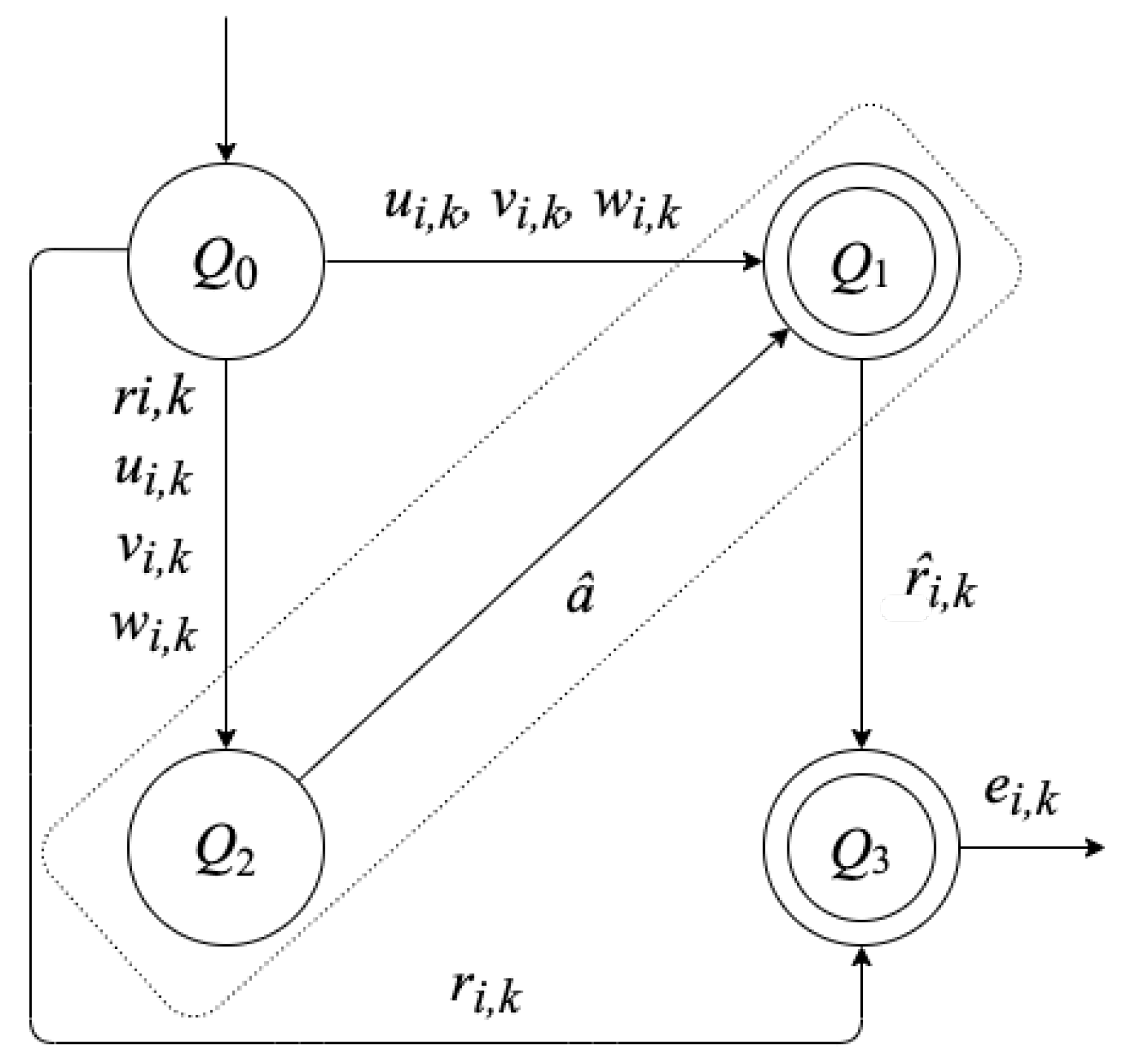
In general, we can say that the reconstruction of the response time dynamics of the instances of a task on RT-Linux depends on the measurement and characterization of the response times in experimental form $Q_0$, the proposal of a model with bounded noise $Q_1$, and the estimation of its parameter $Q_2$. To verify the quality of the reconstruction response time dynamics, it is validated by comparing it with experimental measurements $Q_3$.

In formal terms, the R set can be represented as a diagram of states, as shown in Figure 1. The first state is $Q_0$, for which several experiments to measure response times of instances to execute the same algorithm n times are needed. $Q_1$ state is the response times reconstruction model; in this state, we propose a stochastic recursive model to calculate response times ${\widehat{r}}_{i,k}$ of $j_{i,k}$ instances. $Q_2$ state is a parameter estimator based on a mathematical expectation quotient, and the result of this state is a, which is an input to the $Q_1$ state. Finally, the $Q_3$ state is used to calculate the reconstruction error and to validate our algorithm. Note that $Q_1$ and $Q_2$ states are in a rectangle drawn with a dashed line in Figure 1 to indicate that two states build the response times reconstructor of dynamic response times. Following this context, for each state, we proposed a second level state diagram to represent internal procedures to obtain the respective result.

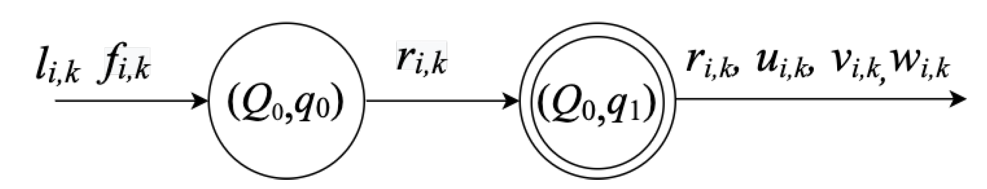
2.1. $Q_0$: Measurement of Response Times

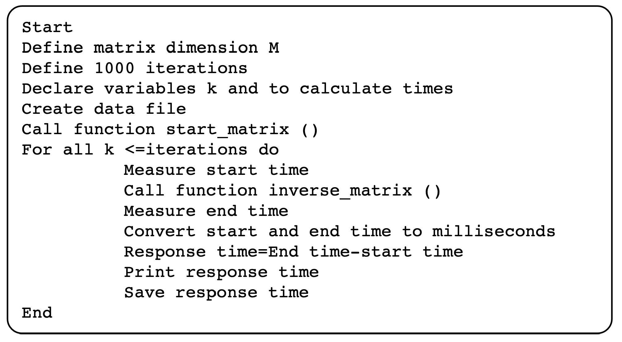
In the $Q_0$ state, the response times are measured by a matrix inversion task with high priority in RT-Linux. The matrix inversion algorithm was previously programmed in C language, as shown the pseudocode in Figure 2. In the algorithm, we use the function sched_setscheduler(), where we specify the Round Robin real-time policy SCHED_RR() and the priority. In this case, we use function sched_get_priority_max() [25] to obtain the highest priority of the scheduler, which returns an integer value of 99.

For times measurement, we use the function clock_gettime() because it has a resolution of nanoseconds. Using these functions, we obtain response times to each instance $j_{i,k}$. This procedure can be represented by the state diagram of Figure 3, and it has three states:

$Q_0=\{(Q_0,q_0),(Q_0,q_1),(Q_0,q_2)\}$

$(Q_0,q_0)$: Calculus of measured response times,

$(Q_0,q_1)$: Obtaining of variables to be modeled.

Figure 3. States diagram $Q_0$ for experimental measurement of response times dynamic.

Figure 3. States diagram $Q_0$ for experimental measurement of response times dynamic.

For each instance $j_{i,k}$, the constraints $l_{i,k}$ and $f_{i,k}$ are measured, then the $q_0$ state is the difference between $f_{i,k}$ and $l_{i,k}$, which are calculated and registered as $r_{i,k}$. Then, we obtain input variables $u_{i,k},v_{i,k},w_{i,k}$, to be modeled.

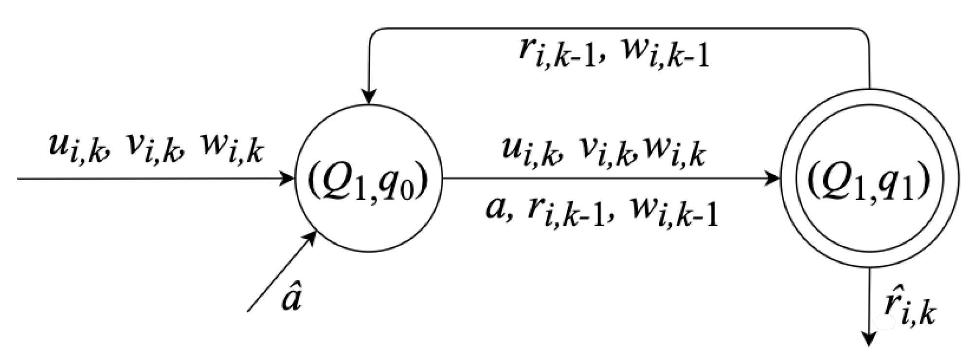
2.2. $Q_1$: Response Times Reconstruction Model

In this part, we propose a set of necessary definitions, a lemma and a theorem to develop the reconstruction model as shown in Figure 4 with the next states.

$Q_1=\{(Q_1,q_0),(Q_1,q_1)\}$

$(Q_1,q_0)$: Reception of system input $u_{i,k}$ internal and external noises $v_{i,k}$, $w_{i,k}$, respectively,

$(Q_1,q_1)$: Calculus of response times reconstruction.

Figure 4. States diagram $Q_1$ for the reconstruction model of response times dynamic.

Figure 4. States diagram $Q_1$ for the reconstruction model of response times dynamic.

To obtain states diagram $Q_1$, it is necessary to formulate Definitions 1 to 4 and propose Lemma 1 and Theorem 1. This diagram includes all the development of this section.

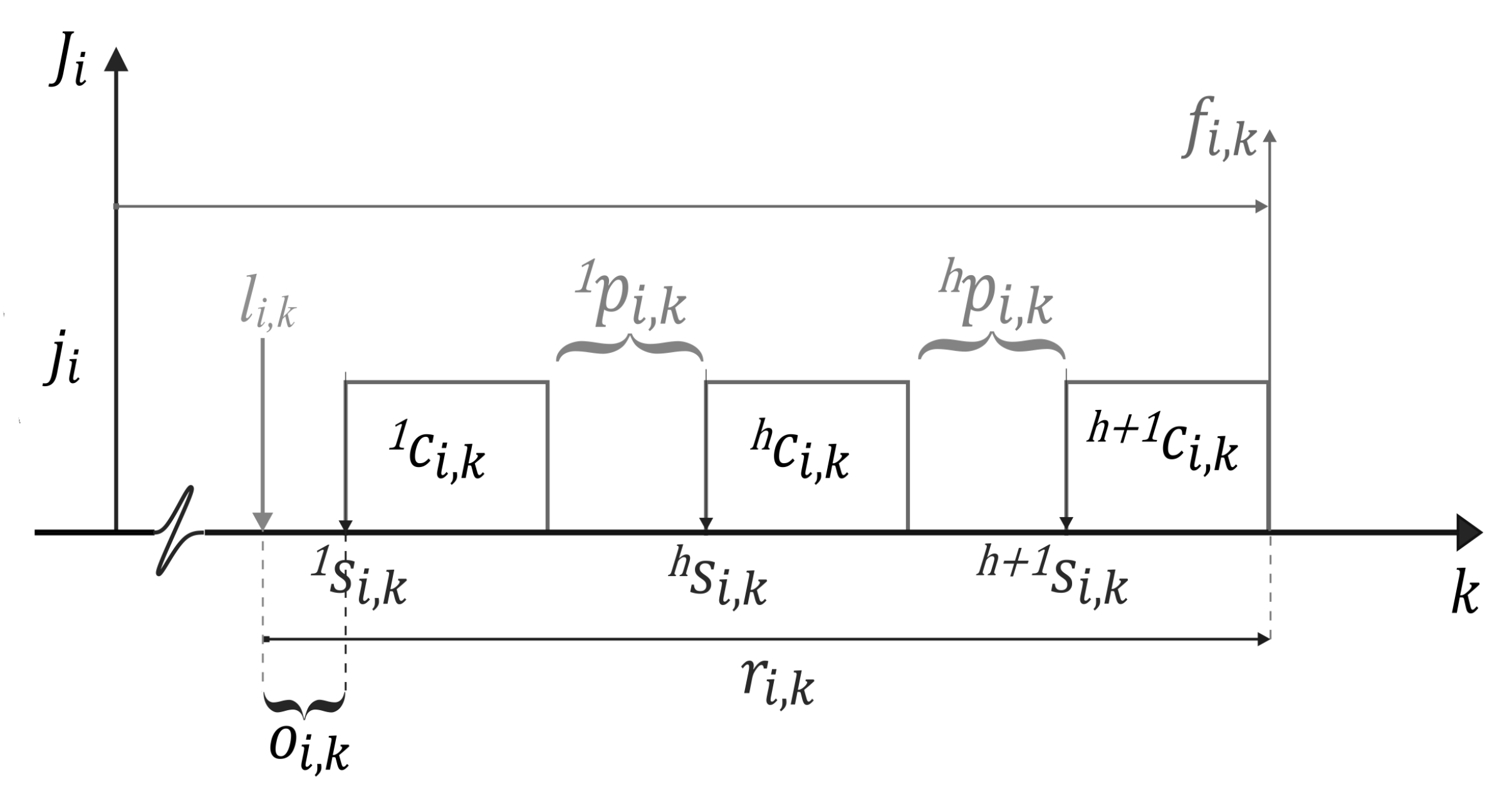
Definition 1

(Response time $r_{i,k}$). The response time of each instance $j_{i,k}$ of a task $J_i$ is computed with:

$$r_{i,k}=f_{i,k}-l_{i,k}$$

(1)

where $r_{i,k},f_{i,k},l_{i,k}\in {\mathbb{R}}^{+}$ and $i,k\in \mathbb{N}.$

The dynamics of response times is considered to be the variation of the response times of the instances of a task, with respect to the temporal evolution of the computational system, considering that all instances execute the same algorithm with fixed high priority. The initial hypothesis is as follows: the dynamics of the response times of a task can be reconstructed from a mathematical model, an estimated parameter and the measurement and characterization of a set of response times of a task with fixed high priority.

Definition 2

(Operation time $o_{i,k}$). Operation time $o_{i,k}$ of a $j_{i,k}$ instance is the elapsed time of the instance since its arrival time, that is: $o_{i,k}=s_{i,k}-l_{i,k}$, with $i,k\in \mathbb{N}.$ $o_{i,k}$ is unique and indivisible for each instance.

Definition 3

(Computing time $c_{i,k}$). Computing time $c_{i,k}$ of a $j_{i,k}$ instance is the time that the instance computes its operations until it finishes, with $i,k\in \mathbb{N}.$

Definition 4

(Preemption time $p_{i,k}$). Preemption time $p_{i,k}$ of a $j_{i,k}$ instance is a temporary interruption of computing time $c_{i,k}$ generated by a higher priority task, with $i,k\in \mathbb{N}$.

Note that an instance $j_{i,k}$ can have a set $p_{i,k}$ of h preemption times during its execution and it has a divided $c_{i,k}$. Thus,

$$p_{i,k}=\sum _{h=1}^{\alpha }{}^h{p}_{i,k}$$

(2)

which implies that

$$c_{i,k}=\sum _{h=1}^{\alpha +1}{}^h{c}_{i,k}$$

(3)

Timing constraints, notation and their relations are based on [1]. In this sense, we present Figure 5, Table 1 and all mathematical development.

Lemma 1.

The response time $r_{i,k}$ of an instance $j_{i,k}$, is the arithmetic sum of operation time $o_{i,k}$ plus computing time $c_{i,k}$ plus preemption time $p_{i,k}$. Thus,

$$r_{i,k}=o_{i,k}+\sum _{h=1}^{\alpha +1}{}^h{c}_{i,k}+\sum _{h=1}^{\alpha }{}^h{p}_{i,k}$$

(4)

$\forall i,k,h,\alpha \in \mathbb{N}$

Proof. 

Considering (3) and substituting in Equation (4):

• $r_{i,k}=o_{i,k}+c_{i,k}+p_{i,k}$
• $o_{i,k}=s_{i.k}-l_{i,k}$
• $r_{i,k}=(s_{i,k}-l_{i,k})+c_{i,k}+p_{i,k}$
• $r_{i,k}=s_{i,k}+c_{i,k}+p_{i,k}-l_{i,k}$

considering $f_{i,k}=s_{i,k}+c_{i,k}+p_{i,k}$ and substituting in previous equation of $r_{i,k}$, we obtain Equation (1)

$r_{i,k}=f_{i,k}-l_{i,k}$ □

With Equations (1) and (4), it is possible to propose a recursive dynamical model [26,27,28]. Therefore, we manage to obtain:

Theorem 1

(Response times dynamic $r_{i,k}$). The response times dynamic of a task with high priority in a stationary system is described as a linear model of first order with a time invariant parameter.

Considering $u_{i,k}$ (system input), a (system parameter), $w_{i,k}$ (external noise) and $v_{i,k}$ (internal noise), the expression of the model is described as follows.

$$r_{i,k}=a[r_{i,k-1}-w_{i,k-1}]+u_{i,k}+v_{i,k}+w_{i,k}$$

(5)

Equation (5) is a linear time-invariant system because the dynamic characterization of the response times of a real-time task with high priority is a recursive model, noise levels are bounded by standard deviation with respect to the response times expectation, and a is an invariant parameter because expectation is considered parallel to the horizontal axis.

Proof. 

Considering Equation (4) $r_i{,}_k=o_{i,k}+c_{i,k}+p_{i,k}$, the behavior of $o_{i,k}$ and $p_{i,k}$ is randomly variable and their magnitudes for each instance indexed by k are different depending on other processes, including the kernel of the operating system. Then, those are random variables of stochastic processes and can be added to obtain:

$$w_{i,k}=o_{i,k}+p_{i,k}$$

(6)

thus,

$$r_{i,k}=c_{i,k}+w_{i,k}$$

(7)

On the other hand, $c_{i,k}$ is an internal state and can not be directly measured. For this reason, we propose a linear equation of first-order with a time invariant parameter, that is:

$$c_{i,k}=a{c}_{i,k-1}+u_{i,k}+v_{i,k}$$

(8)

$u_{i,k}$ is a normalized input with zero mean, $v_{i,k}$ is an internal noise (it could be considered jitter).

Following previous paragraphs, we have to represent $r_{i,k}$ in function of $r_{i,k-1}$ and not to $c_{i,k}$ because we do not know the internal state of the system. Thus, we clear $c_{i,k}$ from Equation (7), and we have the following:

$$c_{i,k}=r_{i,k}-w_{i,k}$$

(9)

Applying a delay to Equation (9), we obtain

$$c_{i,k-1}=r_{i,k-1}-w_{i,k-1}$$

(10)

Substituting the equality of Equations (9) and (10) into Equation (8), we have.

$$r_{i,k}-w_{i,k}=a[r_{i,k-1}-w_{i,k-1}]+u_{i,k}+v_{i,k}$$

(11)

Clearing $r_{i,k}$ from Equation (11), we obtain the model represented by Equation (5)

$r_{i,k}=a[r_{i,k-1}-w_{i,k-1}]+u_{i,k}+v_{i,k}+w_{i,k}$ □

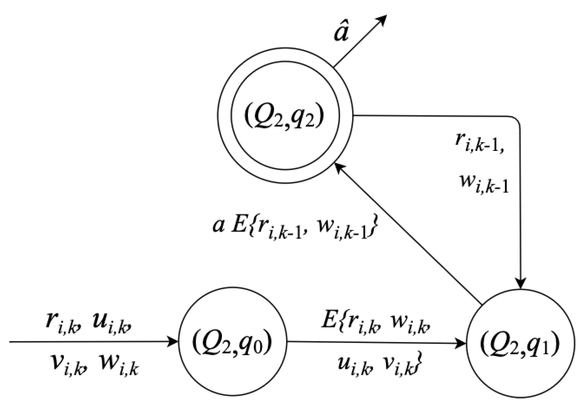
2.3. $Q_2$: Parameter Estimation

An important question about parameters estimation is how to calculate parameter a. Then, for this state, we need to estimate an $\widehat{a}$ as is explained in [5], so that $\widehat{a}\to a$. Figure 6 shows the diagram that describes states to compose estimator ${\widehat{a}}_{i,k}$.

Note that estimation of $\widehat{a}$ is the last value of recursive calculus of ${\widehat{a}}_{i,k}$, such that $\widehat{a}={\widehat{a}}_{i,m}$ for m instances.

$Q_2=\{(Q_2,q_0),(Q_2,q_1),(Q_2,q_2)\}$

$(Q_2,q_0)$: Response time $r_{i,k}$, system input $u_{i,k}$, external and internal noises, $w_{i,k}$, $v_{i,k}$, respectively,

$(Q_2,q_1)$: Response times model,

$(Q_2,q_2)$: Estimation of $\widehat{a}$.

Figure 6. States diagram $Q_2$ for the parameter estimation ${\widehat{a}}_{i,k}$.

Figure 6. States diagram $Q_2$ for the parameter estimation ${\widehat{a}}_{i,k}$.

The goal of $Q_2$ state is to calculate $\widehat{a}$; for this, it is necessary to take into consideration the following conditions:

• $E\left\{w_{i,k}{r}_{i,k-1}\right\}=0$,
• $E\left\{w_{i,k}{r}_{i,k}\right\}={\sigma }_{w_k}^2$,
• $E\left\{v_{i,k}{r}_{i,k}\right\}={\sigma }_{v_k}^2$,
• $E\left\{v_{i,k}{v}_{i,k}\right\}={\sigma }_{v_{i,k}}^2$,
• $E\left\{w_{i,k}{w}_{i,k}\right\}={\sigma }_{w_{i,k}}^2$
• $E\left\{v_{i,k}{w}_{i,k}\right\}=0$

With the conditions above, we can propose the next lemma.

Lemma 2

(Estimator parameter $\widehat{a}$ for response times $r_{i,k}$). The estimator parameter for the model presented in Theorem 1, is described by:

$$\begin{array}{c}\hfill \widehat{a}=\frac{E\left\{r_{i,k}-w_{i,k}-u_{i,k}-v_{i,k}\right\}}{E\left\{r_{i,k-1}-w_{i,k-1}\right\}}\end{array}$$

(12)

Proof. 

Because the system is linear, stationary and first-order, we propose to build an estimator based on the quotient of mathematical expectation. Starting from Equation (11), we apply mathematical expectation to both sides of equality

$$E\left\{r_{i,k}-w_{i,k}-u_{i,k}-v_{i,k}\right\}=aE\left\{r_{i,k-1}-w_{i,k-1}\right\}$$

(13)

and clearing the parameter a, we obtain $\widehat{a}$ as in Equation (12). □

In Figure 1, we explain that $Q_1$ and $Q_2$ states are part of the procedure for times reconstruction. Then, substituting Equation (12) into Equation (5), we obtain the reconstructed response times ${\widehat{r}}_{i,k}$, that is:

$${\widehat{r}}_{i,k}=\widehat{a}[{\widehat{r}}_{i,k-1}-w_{i,k-1}]+u_{i,k}+v_{i,k}+w_{i,k}$$

(14)

Equation (14) is programmed in recursive form and allows to observe the dynamic of ${\widehat{r}}_{i,k}$ through the system evolution. In the same way, we calculate $\widehat{a}$, and the reconstruction of ${\widehat{r}}_{i,k}$ implies that ${\widehat{r}}_{i,k}\to r_{i,k}$. Then, it is possible to know the reconstruction response times error by state $Q_3$.

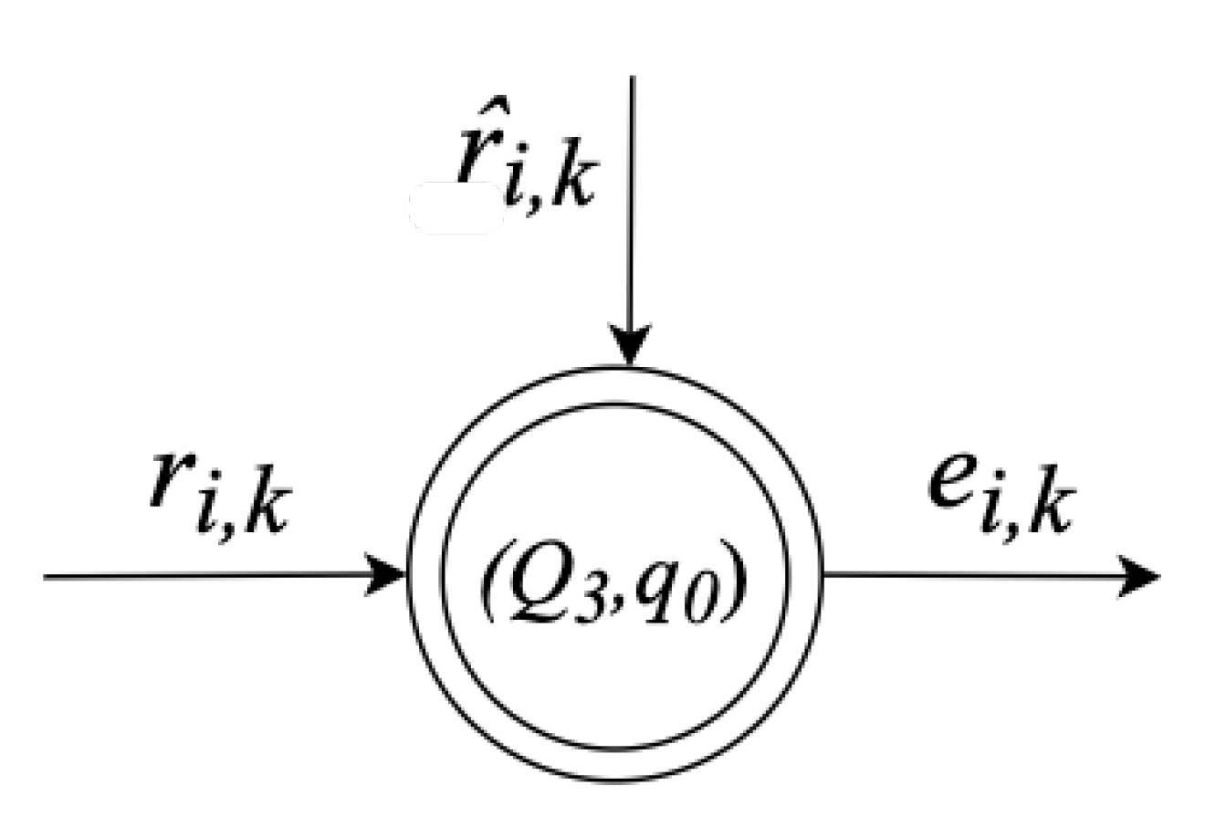
2.4. $Q_3$: Reconstruction Response Times Error

This stage is very important. We validate the quality of the proposed reconstruction model through reconstruction error and mean squared error. For this, we present the third state as is shown in Figure 7:

$Q_3=\left\{(Q_3,q_0)\right\}$

$(Q_3,q_0)$: Calculus of reconstruction response times error $e_{i,k}$

Figure 7. States diagram $Q_3$ for response times reconstruction error of a task with high priority over RT-Linux.

Figure 7. States diagram $Q_3$ for response times reconstruction error of a task with high priority over RT-Linux.

The reconstruction response times error consists of calculating the difference between estimated response time and measured response time (see [29]):

$$e_{i,k}={\widehat{r}}_{i,k}-r_{i,k}$$

(15)

The mean squared error [30] measures how widely the estimator varies to the estimated value itself. We expect an estimator with a lower mean squared error and closer to the measured value we seek to estimate.

$$\mu e_{i,k}^2=E\{(e_{i,k}{)}^2\}$$

(16)

3. Experimental Results

This section presents a compendium of graphs that illustrate the response times measured and reconstructed through the proposed model in the development section. The experiments were carried out over a setup workbench by a single board computer with PREEMPT_RT and a task using the algorithm of matrix inversion programmed on C language. The matrix inversion algorithm as a process was executed implementing a Round-Robin scheduling mechanism with fixed high priority. It is important to mention that FIFO and Round-Robin schedulers were previously tested; the scheduling mechanism was implemented with the sched_setscheduler() function. It was observed that with Round-Robin scheduler there were minor variations compared to FIFO, this was seen in the process of characterizing the first and second probability moments due to the fact that Round-Robin assigns timeslices to each task guaranteeing that the response times behave uniformly in RT-Linux. Nevertheless, we ran the matrix inversion with dimensions 32 × 32, 64 × 64, and 128 × 128 as the test-bench, each up to 1000 instances; hence, we obtain the measures of response times.

Table 2. Test bench elements and their characteristics.

Element	Characteristic
SBC	Raspberry Pi 4, 4 GB
Operating system	RT-Linux (PREEMPT-RT)
Scheduler	Round Robin (SCHED_RR)
Priority	High priority (99)
Algorithm	Matrix inversion

specifies the test bench elements and their characteristics to perform these experiments. It is very important to mention that we consider just one task in the experiments run.

This work is supported by a statistical analysis involving the calculation of the first and second moments of probability. These mathematical tools allow us to know the behavior of the response times during the evolution of the task. As we considered in the development section, by means of the state $Q_1$ and in Theorem 1, the behavior of the response times is described as a stationary and time invariant stochastic system. It is considered a time invariant model because according to the characterization of the measured response times, no large variations in the magnitudes are observed; therefore, a constant parameter $\widehat{a}$ is estimated. Once the response times were measured experimentally, it was observed that the first and second moments of probability remained constant, so the system was considered to be stationary. Furthermore, we present the first model for response times reconstruction based on the measurements and characterization of the system, which is considered linear since the behavior of the response times dynamics remains constant within a bounded range; if the size of the matrix increases, then the magnitude of the response times are growing exponentially, in which complexity is $O\left(n^3\right)$ [24]. Subsequently, we obtained graphs showing results describing the following:

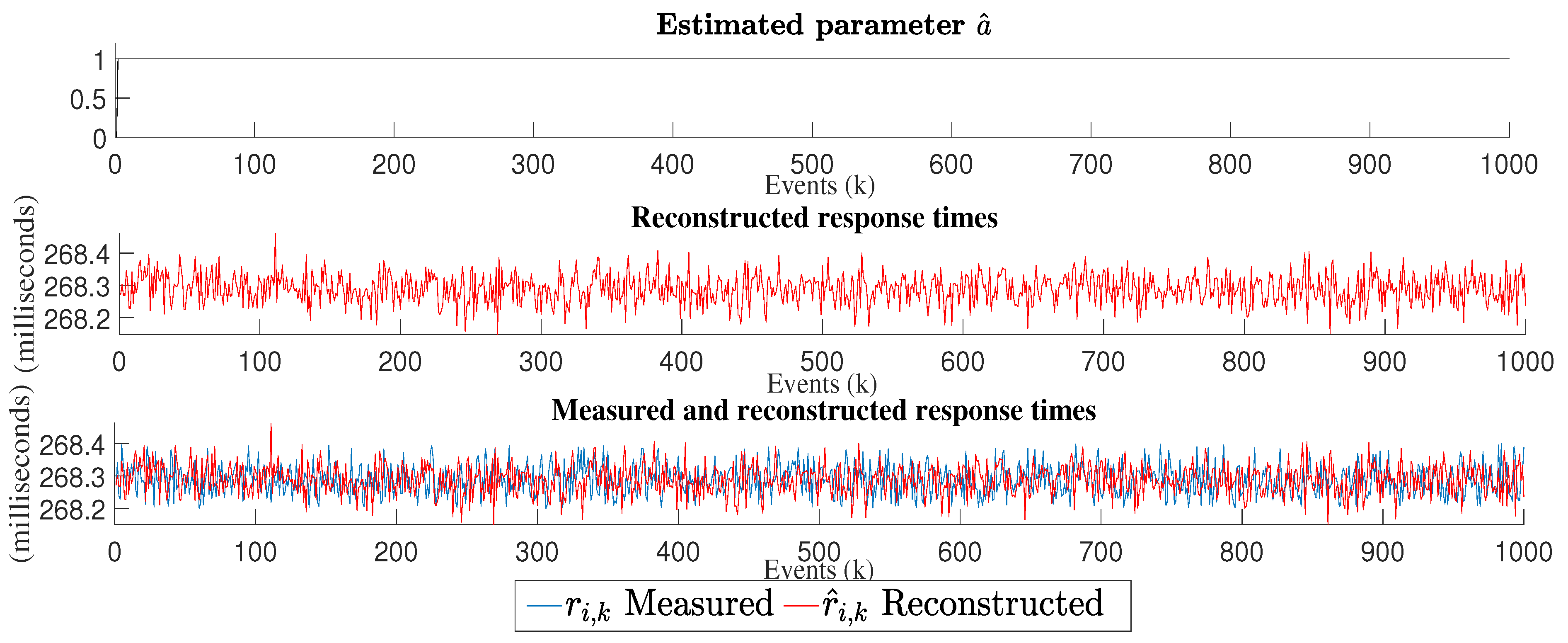
Figure 8, Figure 9 and Figure 10 illustrate three graphs. The first one represents the estimated parameter $\widehat{a}$. The second one shows the result of the reconstructed response times. Finally, in the third one, an overlap is observed between the graphs of measured response times (blue) and the reconstructed response times (red).

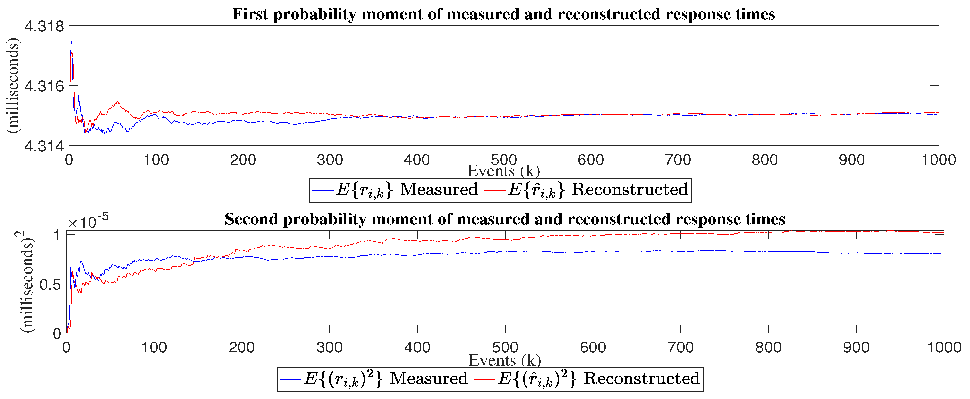
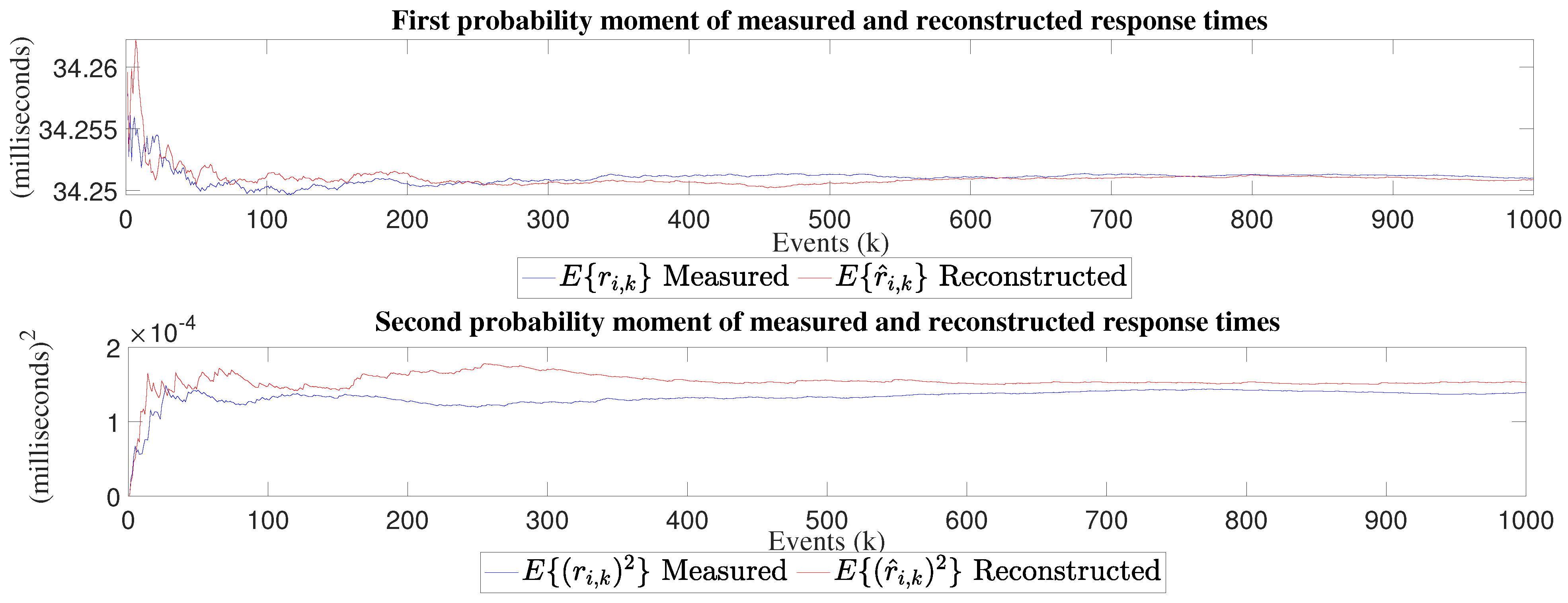
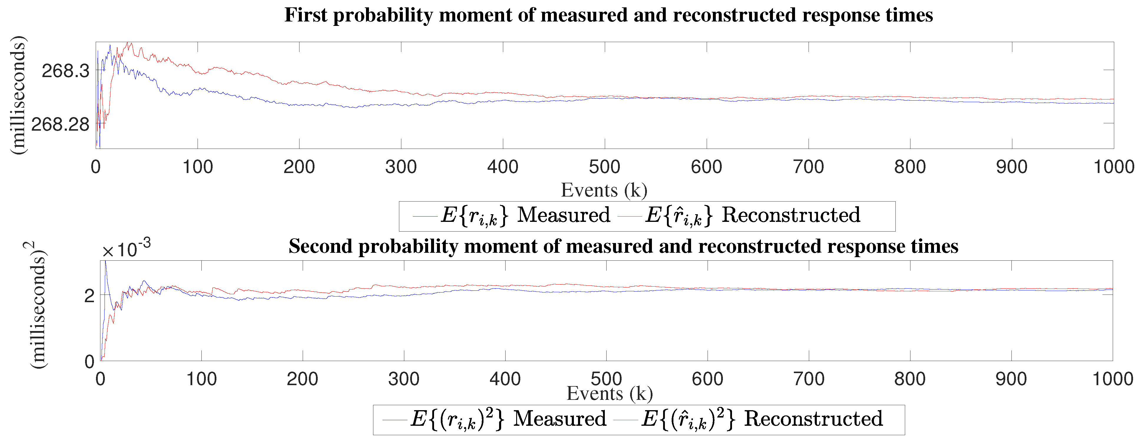
Figure 11, Figure 12 and Figure 13 show first and second probability moments. These figures are very important because convergence can be seen almost everywhere, which validates the proposed model based on the quotient of mathematical expectation.

The model for reconstructing the dynamics of response times has two main uses for future applications: First, sizing the computational system to make optimal use of its memory resources and CPU usage, and second, proposing fault tolerance schemes, since when the magnitude of response times starts to increase or a high variation of the first and second probability moments is observed, the computational system could fail.

4. Discussion

In state $Q_0$, the response times are generated by the computer system aforementioned. From the execution of a matrix inversion algorithm programmed in C language, the time generated by its execution is measured in temporal units, using the clock_gettime() function. In addition to this, the Round-Robin real-time policy and high priority are specified in the sched_set_scheduler() function. Once the response times were measured and stored, we observed that due to the non-polynomial complexity of the matrix inversion algorithm, the response times grew exponentially. Then, in order to know the performance of the system, we proceeded to analyze its behavior by means of its statistical characterization through its first and second moments of probability. Thus, we found that the system behavior is stationary. With this information, we made a theoretical proposal based on a first-order linear model, with a time invariant parameter and bounded noise.

In state $Q_1$, a response times reconstruction model is proposed. However, to obtain it, it was necessary to develop a set of definitions, a lemma and a theorem. We proposed a recursive dynamical model owing to the statistical characterization of measured response times.

In state $Q_2$, due to the characteristics of the system, it was proposed to build an estimator based on the mathematical expectation quotient. This was programmed in a recursive way to observe the dynamics of ${\widehat{r}}_{i,k}$ through the evolution of the system.

In state $Q_3$, the quality of the proposed reconstruction model was validated by calculating its reconstruction error and mean squared error. We observe that both errors are close to zero, which determines that we obtained a good estimation of real measured values.

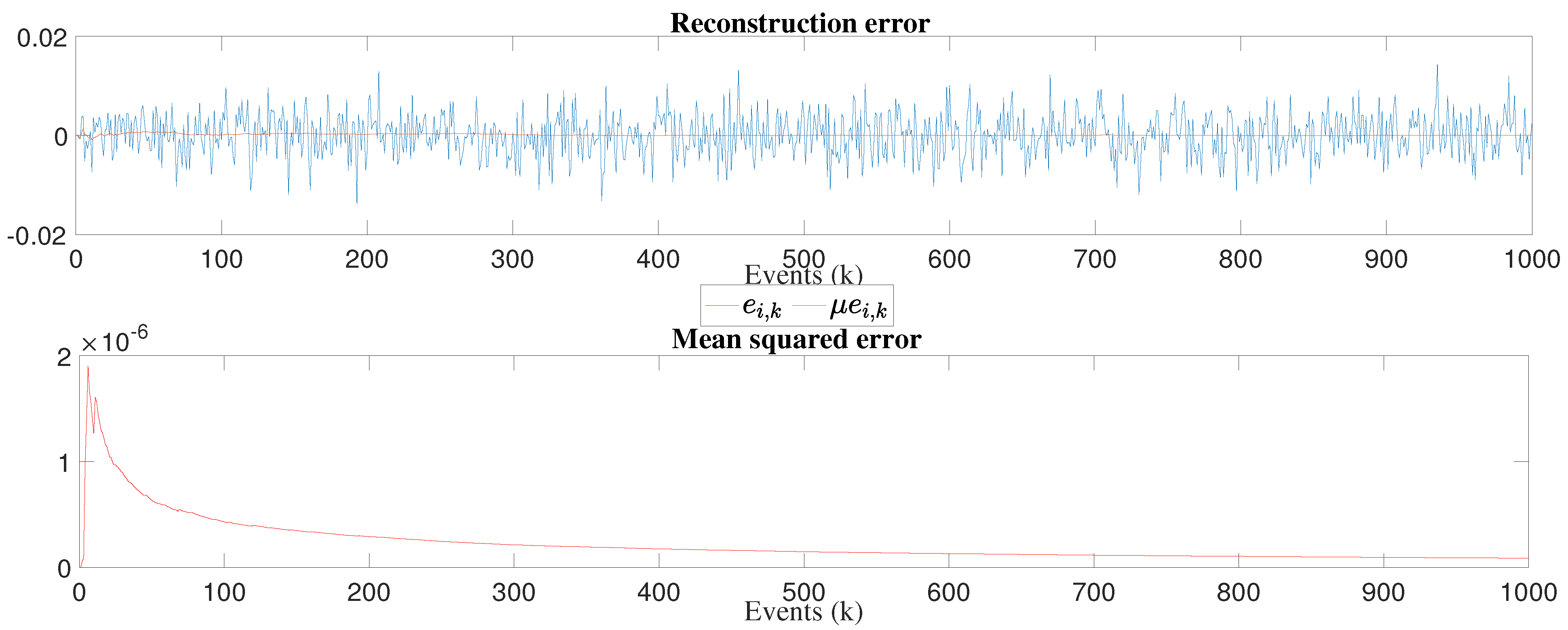
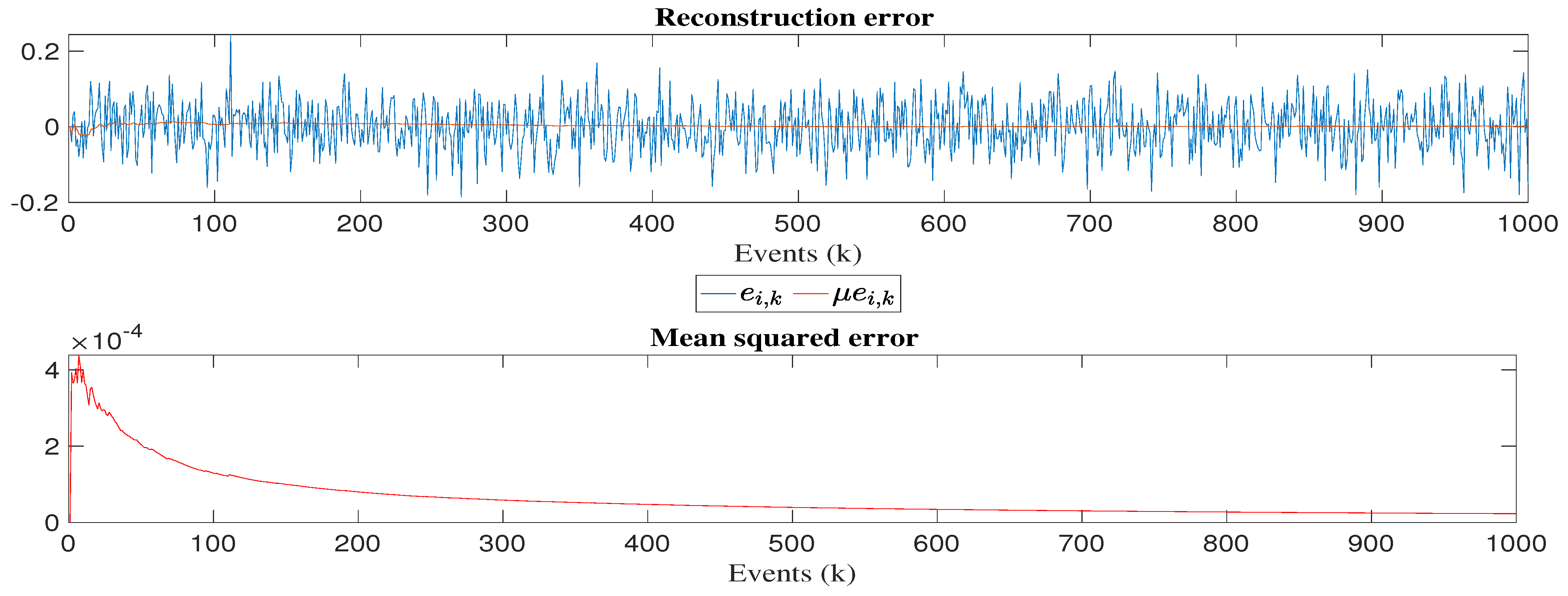
In order to validate the proposed reconstruction model, Figure 14, Figure 15 and Figure 16 show the reconstruction error and mean squared error, where it is observed in all experiments that errors are close to zero. With respect to this, it is confirmed that the proposed model has a good convergence. To thoroughly explain our results, we present a brief discussion of last data values for each experiment in

Table 3. Last values of the first and second probability moments for each experiment.

Last Value	$32\times 32$	$64\times 64$	$128\times 128$
$E\left\{r_{i,k}\right\}$	4.3151 ms	34.2510 ms	268.2875 ms
$E\left\{{\widehat{r}}_{i,k}\right\}$	4.3151 ms	34.2509 ms	268.2890 ms
$E\{{\left(r_{i,k}\right)}^2\}$	8.1334 × 10${}^{-6}$ ms${}^2$	1.39 × 10${}^{-4}$ ms${}^2$	2.1610${}^{-3}$ ms${}^2$
$E\{{\left({\widehat{r}}_{i,k}\right)}^2\}$	1.02 × 10${}^{-5}$ ms${}^2$	1.53 × 10${}^{-4}$ ms${}^2$	2.19 × 10${}^{-3}$ ms${}^2$
$E\left\{e_{i,k}\right\}$	5.05 × 10${}^{-5}$ ms	−1.38 × 10${}^{-4}$ ms	1.5 × 10${}^{-3}$ ms
$E\{(e_{i,k}{)}^2\}$	8.86 × 10${}^{-8}$ ms${}^2$	1.79 × 10${}^{-6}$ ms${}^2$	2.28 × 10${}^{-5}$ ms${}^2$
$\widehat{a}$	0.99	0.9987	0.9998

.

For the 32 × 32 experiment, we can see that the mathematical expectation of the measured and reconstructed response times are the same, i.e., 4.3151 ms, the estimated parameter $\widehat{a}$ converges to 0.99, the variance for measured times is 8.1334 × 10${}^{-6}$ ms${}^2$ and for reconstructed times is 1.02 × 10${}^{-5}$ms${}^2$, its reconstruction error mean is 5.05 × 10${}^{-5}$ ms, the mean squared error value is 8.86 × 10${}^{-8}$ ms${}^2$.

For the 64 × 64 experiment, we can observe that mathematical expectation of measured and reconstructed times has a little bit difference of 0.0001 ms, the estimated parameter $\widehat{a}$ converges to 0.9987, the variance of measured times is 1.39 × 10${}^{-4}$ ms${}^2$ and for reconstructed times is 1.53 × 10${}^{-4}$ ms${}^2$, its reconstruction error mean is −1.38 × 10${}^{-4}$ ms, the mean squared error value is 1.79 × 10${}^{-6}$ ms${}^2$.

For the 128 × 128 experiment, the mathematical expectation of measured times is 268.2875 ms, while for the reconstructed times, we obtained 268.2890 ms, its estimated parameter $\widehat{a}$ converges to 0.9998, the variance of measured times is 2.1610 × 10${}^{-3}$ ms${}^2$ and for reconstructed times is 2.19 × 10${}^{-3}$ ms${}^2$, its reconstruction error mean is 1.5 × 10${}^{-3}$ ms, the mean squared error value is 2.28 × 10${}^{-5}$ ms${}^2$.

It can be clearly seen that estimated parameter a is always lower than 1. This is because response times dynamic is stable all the time, otherwise it could not be reconstructed. If the last value were 1, our reconstruction would be very inaccurate since the system could be considered as marginally stable. If it exceeded the value of 1 it would be totally unstable and it would be practically impossible to achieve a good approximation of the real measured values.

5. Conclusions

In this paper, it was necessary a set up a workbench by a single board computer Raspberry Pi 4, PREEMPT_RT Linux kernel, and a matrix inversion task programmed in C language. The whole development of this paper is basically represented in a diagram composed of four states, from response times measuring $Q_0$ to validation of the proposed model with reconstruction error calculus $Q_3$.

In this paper, we made the following contributions:

• We developed the needed theory for response times dynamic.
• The development of a model for response times reconstruction of a high priority task over RT-Linux was carried out.
• The development of a parameter estimator for the proposed model based on the quotient of mathematical expectation works properly according to the obtained reconstruction error response.
• Experimental validation of the proposed model through a real task running with high priority over RT-Linux was performed.

The scenario proposed in this paper is stable, applicable to high priority tasks in a non-proprietary real-time operating system such as RT-Linux. The use of the model and reconstruction can be focused on applications that require implementing periodic tasks, iterative algorithms, or models that use matrix operations exhaustively, where there is a need to improve computational performance and algorithmic efficiency with RT-Linux on an SBC such as Raspberry Pi; for example, in [31].

Modeling allows us to mathematically represent the behavior of the system, giving us an idea of how it could behave in different scenarios and leading us to know the worst ones. In the case of real-time systems, it is quite significant to custom make them for specific applications to know how they would behave in stressful situations by giving them a high computational load and using real-time priorities. That was the main reason for this work. We are satisfied with the results; however, another reconstruction estimation technique can be proposed that could have a better approximation. For future work, it would be interesting to propose a multivariate model involving the simultaneous execution of more than one task and, moreover, to propose other estimation and modeling techniques, perhaps using the Kalman filter, the instrumental variable, and fuzzy logic, among others.

Finally, comparing this work with the results reported in the state-of-the-art, most of the models served as a basis for this work but do not perform the experimental analysis. It is very important to highlight the development of a dynamic model capable of describing the behavior of the response times of the set of instances $j_{i,k}$ of a task $J_i$ with high priority on a RT-linux system and not only a qualitative description through a statistical analysis as presented by the cited authors, since the aim of their work is not to reconstruct the system, but to describe it statistically according to their qualities.