
On the Double Roman Domination in Generalized Petersen Graphs P(5k,k)


Abstract
1. Introduction
2. Preliminaries
2.1. Graphs and Double Roman Domination
- (1)
- every vertex u with is adjacent to at least one vertex assigned 3 or at least two vertices assigned 2, and
- (2)
- every vertex u with is adjacent to at least one vertex assigned 2 or 3 under f.
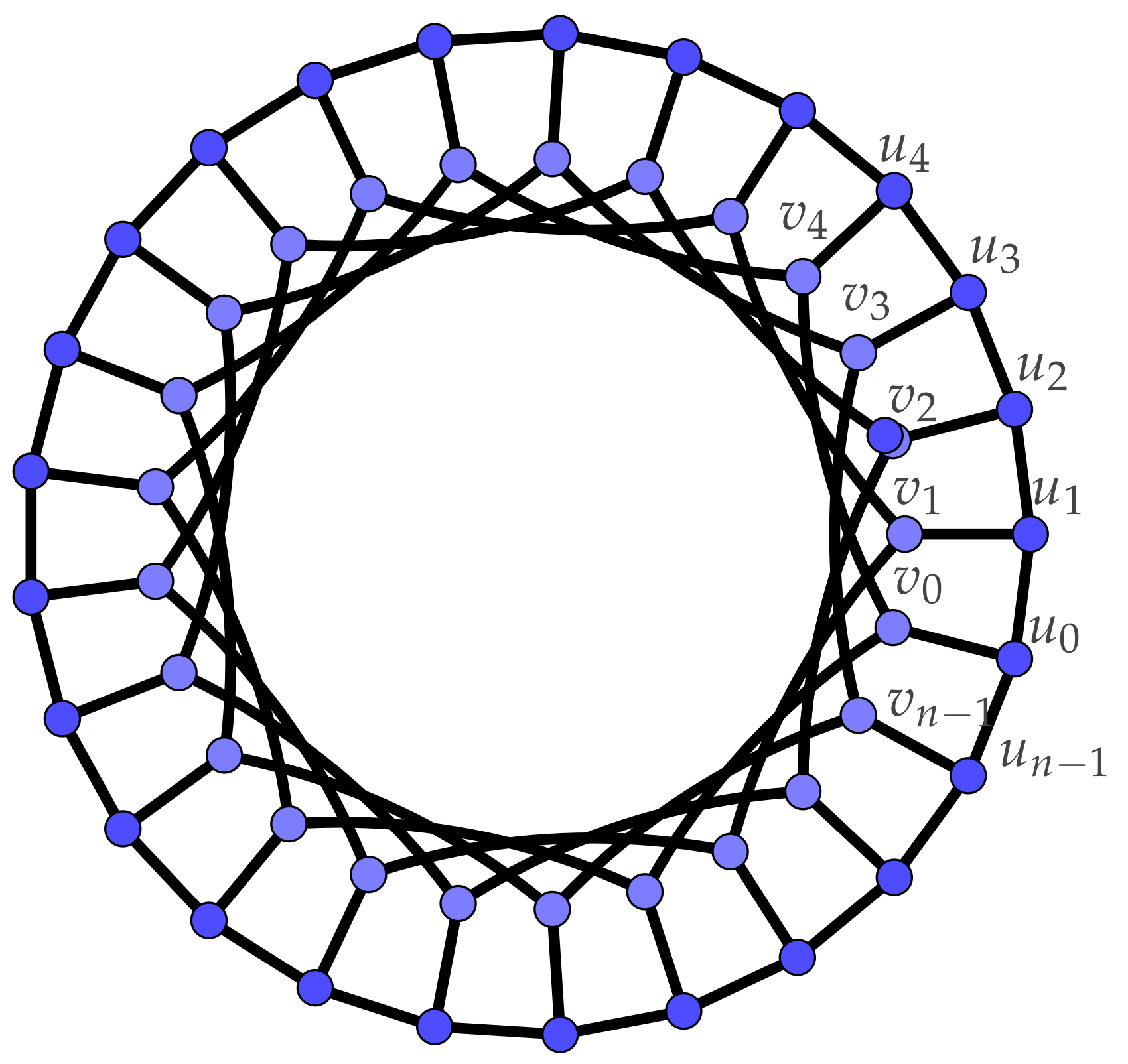
2.2. Generalized Petersen Graphs
2.3. Related Previous Work
2.4. Our Results
3. Constructions and Proofs
3.1. Basic Constructions for
- First, note that the columns in Table 4 have the following properties: each column has two consecutive vertices that are assigned two legions: say and for some i. Then, in the column i, vertices and have one neighbor and the vertex has two neighbors in the outer cycle that are assigned 2. Clearly, the missing legions can be provided by assigning weight 2 to vertices and on the inner cycle. In this assignment, each of the vertices , and is adjacent to two vertices of weight 2. Hence we have weight 8 for each column.
- Second, observe that columns 2 and 7 coincide. Recalling the convention given in Table 3, note that for , column 2 is column 0 shifted one row upwards (cyclicaly). Similarly, for , and columns 0 and 7.
3.2. Double Roman Domination in —Upper Bounds
3.3. Double Roman Domination in —Lower Bound
- Case . First, assume . Excluding weights 1, the sum 9 can be achieved as or . In the first case, three vertices among five can be chosen in two ways, either the two zeros are at adjacent columns or not. Similarly, in the second case, the 0 can either be next to 3, or not. Thus, we have 4 cases listed below. The values on are chosen so that the total weight is minimal.In all cases we have , thusFurthermore, if or then observe that , and hence .
- Case . Possible subcases with areandIn all cases, , thus
- Case . There is only one possibility, , and we have the following subcases:It is obvious that and
- Case . This sum can be achieved as There are four subcases:In all cases the value is at least 3, which implies
- Case . We have , and two possibilities.Clearly, in both cases must be at least 4, which implies
- Case . As , we have two cases:As in both cases, we have
- Case . There is only one possible subcase with , thus
- Case . The only possible subcase is with , thus
- Case has two possible subcases,with , thus
- (a)
- If and then and .
- (b)
- If and then and .
- (c)
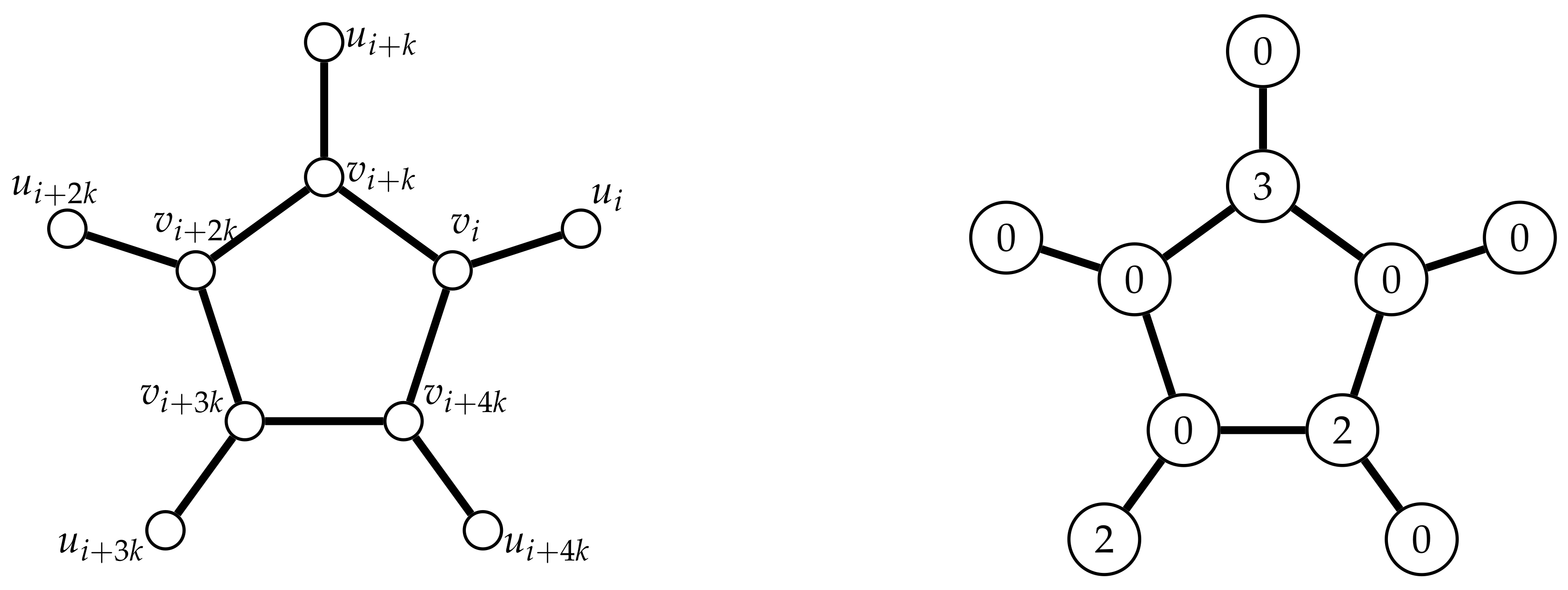
- If and then , , and .
- (a)
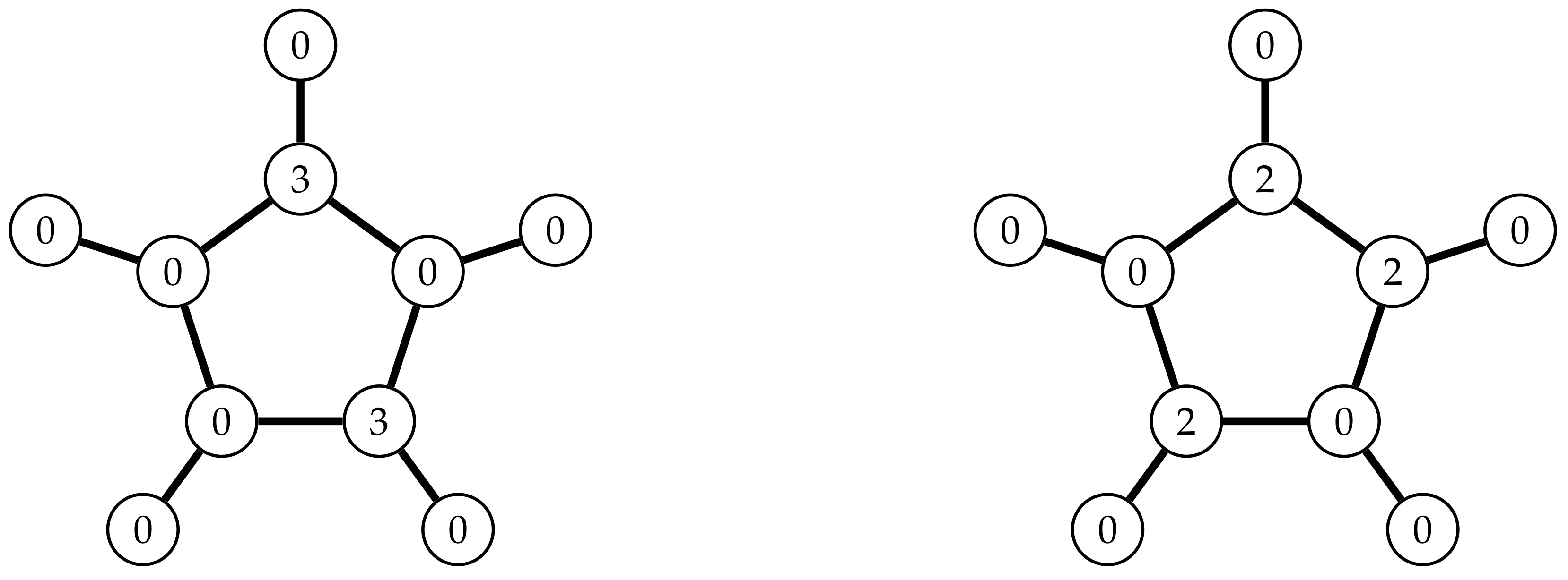
- Case and obviously implies that and . There are two cases (see Figure 3), for which Table 9 (columns A1 and A2) show the minimal demands that the two neighboring vertices in have to fulfil. Without loss of generality, consider first . Since , we read from Table 9 that at least three vertices of must have weights 3, thus and By analogous reasoning,
- (b)
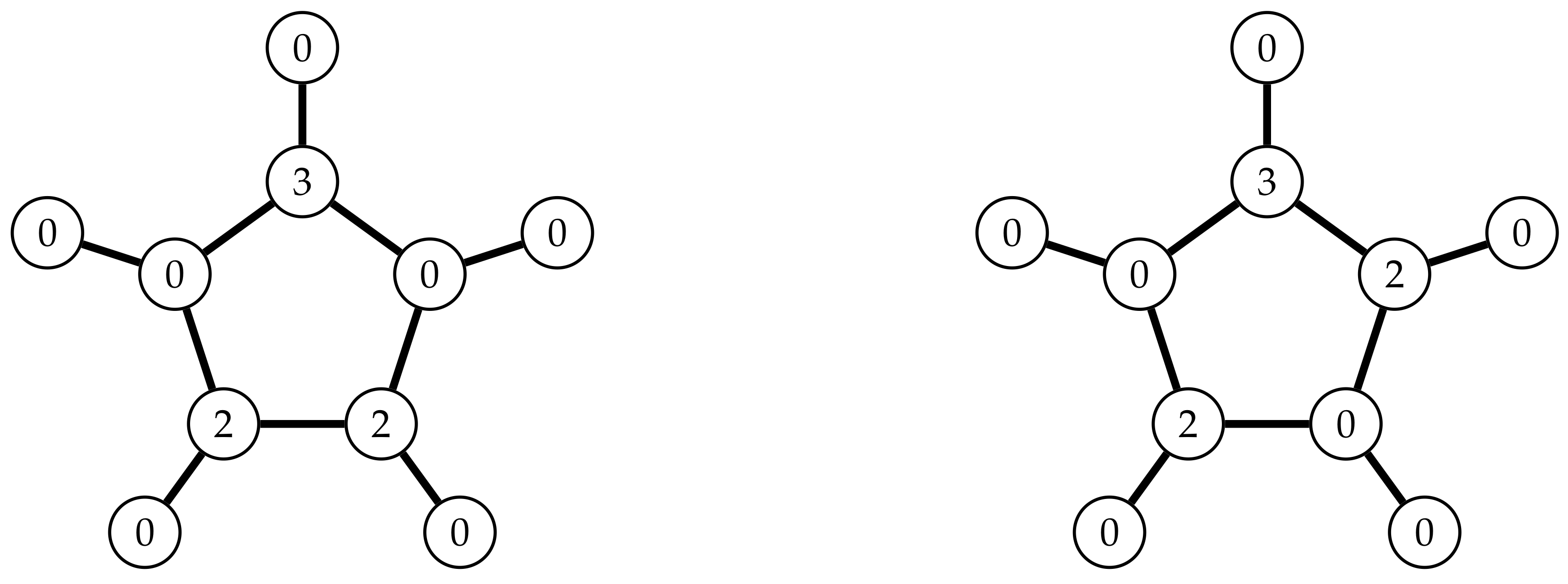
- Case and (see Figure 4). First, consider the case when . Then, from Table 9 (columns A3 and A4) there are at least two vertices of which must have weights 3, and two more vertices with weights at least two, thus and By symmetry, impliesTherefore, we may assume that and . The DRDF for is in Figure 2 (right). Considering neighbor sets and we have all subcases listed in Table 10 and Table 11.In Table 10 and Table 11, we fix DRDF on (second column), and consider all possible DRDF with and (third column). The first and fourth columns provide the minimal f values in and , respectively. The labeled graph in this case has no symmetries, hence we have to consider five rotations, and in each case two cases due to reflexion. Thus, we have ten cases in total, b1 to b10, outlined in Table 10 and Table 11.
- (c)
- Case and . First, observe that in the case when , the reasoning in case (a) and (b) implies that and . So we can assume that . As seen in Figure 3, three vertices in could have weights 2 or two of them have weights 3. As we know, one vertex in has weight 3 and the other one (two steps further) has weight 2, see Figure 2. We thus fix the assignment in (second column), add all possible assignments in (third column) and write the minimal weights on and in the first and fourth column. As each of the two assignments of is reflexion symmetric, it is clear that there are exactly 10 different cases. All possible outcomes for sets are given below, Table 12 and Table 13.In Table 12, we find all subcases (c1 to c5) when two vertices in have weights 3.In Table 13, we have all subcases (c6 to c10) when three vertices in have weights 2.
- (a)
- If and then either ()or (, , and ).
- (b)
- If and then either ()or ( and ).
- (a)
- Case implies (Figure 3). Recall that either three vertices in have weight 2 or two of them have weight 3, and that Table 9 gives the demands that need to be fulfilled by the neighboring . As and , according to lemma 1, we have and . We may also assume that . Thus, we have , and all cases are analyzed in Table 14, Table 15 and Table 16. Note that there is only one case for (and ), because if then .Reading Table 14 we observe that weights are (A1-1) , , (A1-2) , , (A1-3) , , (A1-4) , , (A1-5) , , (A1-6) , , (A1-7) , , (A1-8) , , so in cases (A1-6), (A1-7), and (A1-8), . However, in the first five cases (labelled with asterisk), , and therefore we need to consider and to conclude the proof of assertion (a) of Lemma 3, see Table 15.From Table 15 we can estimate weights (A1-1) , , , , (A1-2) , , , , (A1-3) , , , , (A1-4) , , , , (A1-5) , , , . Here, in all cases, , and .Reading Table 16 we observe that (A2-1) , , (A2-2) , , (A2-3) , , (A2-4) , , (A2-5) , , (A2-6) , , (A2-7) , , (A2-8) , , (A2-9) , , (A2-10) , , (A2-11) , , (A2-12) , , (A2-13) , , (A2-14) , , (A2-15) , , so in all cases , which proves the assertion (a) of Lemma 3.
- (b)
- Case . First, assume that (see Figure 2), so one vertex in has weight 3 and the other one has weight 2. Possible (due to symmetry) solutions for the whole set are considered in the following Table 17.Without loss of generality, assume that . As and we have the following subcases (see Table 18).Reading Table 18 we observe that in all cases except one (B1-4) we have . Indeed, in (B1-1) , , (B1-2) , , (B1-3) , , (B1-4) , , (B1-5) , , (B1-6) , . In case (B1-4) we need to consider weights on and to conclude the proof of assertion (b) of Lemma 3.As seen from Table 19, in case (B1-4) we can confirm and .Finally, if (see Figure 4), then observe that in comparison to the case , there must be at least one more vertex of weight 2 in . We omit detailed analysis of the cases that confirm .
- (a)
- If and then and . After discharging, and , as needed.
- (b)
- If and then and . After discharging we have and .
- (c)
- If and then , , and . Assume that , . After the first round of discharging, we get and . However, after the second round of discharging, we have .If , , then observe that already and .
- (a)
- and , . If , then , and we are done. Otherwise, by Lemma 3, , , and . Assume that and distinguish two cases.
- (a11)
- and . In the first round of discharging, receives from , and In the second round of discharging, again receives from , and in total receives charge 1 from the left side.
- (a12)
- and . After the first round of discharging, In the second round of discharging, sends to its neighbors. Thus, receives from the left side.
Recall that by Lemma 3, implies , and distinguish two cases.- (a21)
- and . In the first round of discharging, receives from , and In the second round of discharging, again receives from , so in total receives charge from the right side.
- (a22)
- and . After the first round of discharging, In the second round of discharging, receives charge 1 from , and also Thus, after the third round , and, in the fourth round receives charge from . So, in total receives charge from the right side.
Summarizing, receives charge at least from the left side, and at least from the right side. Hence , as claimed. - (b)
- and . If then , as needed. Otherwise, and . We now show that implies that will in two rounds receive at least charge from the left side. Consider two cases.
- (b1)
- . In the first round of discharging, receives from the left side.
- (b2)
- If , then . After the first round of discharging, In the second round of discharging, sends at least to its neighbors.
Thus, receives at least from the left side. By analogous reasoning, implies that receives at least from the right side. Consequently, in total receives at least , as claimed.
4. Domination in Generalized Petersen Graphs
5. Conclusions and Future Work
- Find closed expressions or good lower and upper bounds for . Which graphs among are double Roman?
- The method used here to improve bounds for using and may be used to improve bounds for for larger c.
- Can the small gaps between lower and upper bounds for (and, also for ) be resolved by finding and proving exact values?
Author Contributions
Funding
Institutional Review Board Statement
Informed Consent Statement
Data Availability Statement
Acknowledgments
Conflicts of Interest
References
- Beeler, R.A.; Haynes, T.W.; Hedetniemi, S.T. Double Roman domination. Discrete Appl. Math. 2016, 211, 23–29. [Google Scholar] [CrossRef]
- Cockayne, E.J.; Dreyer, P.A., Jr.; Hedetniemi, S.M.; Hedetniemi, S.T. Roman domination in graphs. Discret. Math. 2004, 278, 11–22. [Google Scholar] [CrossRef]
- ReVelle, C.S.; Rosing, K.E. Defendens Imperium Romanum: A classical problem in military strategy. Am. Math. Mon. 2000, 107, 585–594. [Google Scholar] [CrossRef]
- Stewart, I. Defend the Roman Empire! Sci. Am. 1999, 281, 136–138. [Google Scholar] [CrossRef]
- Arquilla, J.; Fredricksen, H. “Graphing”—An Optimal Grand Strategy. Mil. Oper. Res. 1995, 1, 3–17. [Google Scholar] [CrossRef]
- Hening, M.A. Defending the Roman Empire from Multiple Attacks. Discret. Math. 2003, 271, 101–115. [Google Scholar] [CrossRef][Green Version]
- Ahangar, H.A.; Chellali, M.; Sheikholeslami, S.M. On the double Roman domination in graphs. Discret. Appl. Math. 2017, 232, 1–7. [Google Scholar]
- Barnejee, S.; Henning, M.A.; Pradhan, D. Algorithmic results on double Roman domination in graphs. J. Comb. Optim. 2020, 39, 90–114. [Google Scholar]
- Poureidi, A.; Rad, N.J. On algorithmic complexity of double Roman domination. Discret. Appl. Math. 2020, 285, 539–551. [Google Scholar]
- Zhang, X.; Li, Z.; Jiang, H.; Shao, Z. Double Roman domination in trees. Inf. Process. Lett. 2018, 134, 31–34. [Google Scholar] [CrossRef]
- Poureidi, A. A linear algorithm for double Roman domination of proper interval graphs. Discret. Math. Algorithms Appl. 2020, 12, 2050011. [Google Scholar] [CrossRef]
- Gao, H.; Huang, J.; Yang, Y. Double Roman Domination in Generalized Petersen Graphs. Bull. Iran. Math. Soc. 2021, 1–10. [Google Scholar] [CrossRef]
- Jiang, H.; Wu, P.; Shao, Z.; Rao, Y.; Liu, J. The double Roman domination numbers of generalized Petersen graphs P(n, 2). Mathematics 2018, 6, 206. [Google Scholar] [CrossRef]
- Shao, Z.; Wu, P.; Jiang, H.; Li, Z.; Žerovnik, J.; Zhang, X. Discharging approach for double Roman domination in graphs. IEEE Acces 2018, 6, 63345–63351. [Google Scholar] [CrossRef]
- Shao, Z.; Erveš, R.; Jiang, H.; Peperko, A.; Wu, P.; Žerovnik, J. Double Roman graphs in P(3k, k). Mathematics 2021, 9, 336. [Google Scholar] [CrossRef]
- Amjadi, J.; Nazari-Moghaddam, S.; Sheikholeslami, S.M.; Volkmann, L. An upper bound on the double Roman domination number. J. Comb. Optim. 2018, 36, 81–89. [Google Scholar] [CrossRef]
- Maimani, H.R.; Momeni, M.; Mahid, F.R.; Sheikholeslami, S.M. Independent double Roman domination in graphs. AKCE Int. J. Graphs Comb. 2020, 17, 905–910. [Google Scholar] [CrossRef]
- Mobaraky, B.P.; Sheikholeslami, S.M. Bounds on Roman domination numbers of graphs. Mat. Vesnik 2008, 60, 247–253. [Google Scholar]
- Volkmann, L. Double Roman domination and domatic numbers of graphs. Commun. Comb. Optim. 2018, 3, 71–77. [Google Scholar]
- Garey, M.R.; Johnson, D.S. Computers and Intractability: A Guide to the Theory of NP-Completeness; W. H. Freeman and Co.: San Francisco, CA, USA, 1979. [Google Scholar]
- Haynes, H.W.; Hedetniemi, S.; Slater, P. Fundamentals of Domination in Graphs; Marcel Dekker: New York, NY, USA, 1998. [Google Scholar]
- Haynes, H.W.; Hedetniemi, S.; Slater, P. Domination in Graphs: Advanced Topics; Marcel Dekker: New York, NY, USA, 1998. [Google Scholar]
- Ore, O. Theory of Graphs; American Mathematical Society: Providence, RI, USA, 1967. [Google Scholar]
- Henning, M.A. A Characterization of Roman trees. Discuss. Math. Graph Theory 2002, 22, 325–334. [Google Scholar] [CrossRef]
- Liu, C.H.; Chang, G.J. Upper bounds on Roman domination numbers of graphs. Discret. Math. 2012, 312, 1386–1391. [Google Scholar] [CrossRef]
- Liu, C.H.; Chang, G.J. Roman domination on 2-connected graphs. SIAM J. Discret. Math. 2012, 26, 193–205. [Google Scholar] [CrossRef]
- Pavlič, P.; Žerovnik, J. Roman domination number of the Cartesian products of paths and cycles. Electron. J. Comb. 2012, 16, P19. [Google Scholar] [CrossRef]
- Steimle, A.; Staton, W. The isomorphism classes of the generalized Petersen graphs. Discret. Math. 2009, 309, 231–237. [Google Scholar] [CrossRef]
- Watkins, M.E. A theorem on Tait colorings with an application to the generalized Petersen graphs. J. Comb. Theory 1969, 6, 152–164. [Google Scholar] [CrossRef]
- Behzad, A.; Behzad, M.; Praeger, C.E. On the domination number of the generalized Petersen graphs. Discret. Math. 2008, 308, 603–610. [Google Scholar] [CrossRef][Green Version]
- Ebrahimi, B.J.; Jahanbakht, N.; Mahmoodian, E.S. Vertex domination of generalized Petersen graphs. Discret. Math. 2009, 309, 4355–4361. [Google Scholar] [CrossRef]
- Fu, X.; Yang, Y.; Jiang, B. On the domination number of generalized Petersen graphs P(n, 2). Discret. Math. 2009, 309, 2445–2451. [Google Scholar] [CrossRef]
- Liu, J.; Zhang, X. The exact domination number of generalized Petersen graphs P(n, k) with n=2k and n=2k+2. Comput. Appl. Math. 2014, 33, 497–506. [Google Scholar] [CrossRef]
- Tong, C.; Lin, X.; Yang, Y.; Luo, M. 2-rainbow domination of generalized Petersen graphs P(n, 2). Discret. Appl. Math. 2009, 157, 1932–1937. [Google Scholar] [CrossRef]
- Xu, G. 2-rainbow domination in generalized Petersen graphs P(n, 3). Discret. Appl. Math. 2009, 157, 2570–2573. [Google Scholar] [CrossRef]
- Yan, H.; Kang, L.; Xu, G. The exact domination number of the generalized Petersen graphs. Discret. Math. 2009, 309, 2596–2607. [Google Scholar] [CrossRef][Green Version]
- Zhao, W.; Zheng, M.; Wu, L. Domination in the generalized Petersen graph P(ck, k). Util. Math. 2010, 81, 157–163. [Google Scholar]
- Wang, H.; Xu, X.; Yang, Y. On the Domination Number of Generalized Petersen Graphs P(ck, k). ARS Comb. 2015, 118, 33–49. [Google Scholar]
- Gross, J.L.; Tucker, T.W. Topological Graph Theory; Wiley-Interscience: New York, NY, USA, 1987. [Google Scholar]
- Malnič, A.; Pisanski, T.; Žitnik, A. The clone cover. Ars Math. Contemp. 2015, 8, 95–113. [Google Scholar] [CrossRef]
- Gabrovšek, B.; Peperko, A.; Žerovnik, J. Independent Rainbow Domination Numbers of Generalized Petersen Graphs P(n,2) and P(n, 3). Mathematics 2020, 8, 996. [Google Scholar] [CrossRef]


| ... | ... | ... | ||||||
| ... | ... | ... | ||||||
| ... | ... | ... | ||||||
| ... | ... | ... | ||||||
| 0 | 1 | ... | i | ... | k | ... |
| 0 | 0 | 3 | 0 | 0 | 0 | 3 | 0 | ... |
| 0 | 0 | 0 | 3 | 0 | 0 | 0 | 3 | ... |
| 3 | 0 | 0 | 0 | 3 | 0 | 0 | 0 | ... |
| 0 | 3 | 0 | 0 | 0 | 3 | 0 | 0 | ... |
| 0 | 1 | 2 | 3 | 4 | 5 | 6 | 7 | ... |
| ... | ... | ... | ||||||
| ... | ... | ... | ||||||
| ... | ... | ... | ||||||
| ... | ... | ... | ||||||
| ... | ... | ... | ||||||
| 0 | 1 | ... | i | ... | k | ... |
| 2 | 0 | 2 | 0 | 0 | 2 | 0 | 2 | ... | |
| 2 | 0 | 0 | 2 | 0 | 2 | 0 | 0 | ... | |
| 0 | 2 | 0 | 2 | 0 | 0 | 2 | 0 | ... | |
| 0 | 2 | 0 | 0 | 2 | 0 | 2 | 0 | ... | |
| 0 | 0 | 2 | 0 | 2 | 0 | 0 | 2 | ... | |
| 0 | 1 | 2 | 3 | 4 | 5 | 6 | 7 | 8 | ... |
| 2 | 0 | 0 | 2 | 0 | 2 | 0 | 0 | 2 | ... |
| 2 | 0 | 2 | 0 | 0 | 2 | 0 | 2 | 0 | ... |
| 0 | 0 | 2 | 0 | 2 | 0 | 0 | 2 | 0 | ... |
| 0 | 2 | 0 | 0 | 2 | 0 | 2 | 0 | 0 | ... |
| 0 | 2 | 0 | 2 | 0 | 0 | 2 | 0 | 2 | ... |
| 0 | 1 | 2 | 3 | 4 | 5 | 6 | 7 | 8 | ... |
| 2 | 0 | 2 | 2 | 0 | 2 | ... | |
| 2 | 0 | 0 | 2 | 0 | 0 | ... | |
| 0 | 2 | 0 | 2 | 2 | 0 | ... | |
| 0 | 2 | 0 | 0 | 2 | 0 | ... | |
| 0 | 0 | 2 | 0 | 0 | 2 | ... | |
| 0 | 1 | 2 | 3,4,5 | 6 | 7 | ... | merged columns |
| 0 | 1 | 2 | 3 | 4 | 5 | ... | columns renamed |
| 2 | 0 | 0 | 2 | 0 | 2 | 0 | 2 | 0 | 0 | 2 | ... |
| 2 | 0 | 2 | 0 | 2 | 0 | 0 | 2 | 0 | 2 | 0 | ... |
| 0 | 0 | 2 | 0 | 2 | 0 | 2 | 0 | 0 | 2 | 0 | ... |
| 0 | 2 | 0 | 2 | 0 | 0 | 2 | 0 | 2 | 0 | 0 | ... |
| 0 | 2 | 0 | 2 | 0 | 2 | 0 | 0 | 2 | 0 | 2 | ... |
| 0 | 1 | 2 | 3’ | 2’ | 3 | 4 | 5 | 6 | 7 | 8 | ... |
| 0 | 1 | 2 | 3 | 4 | 5 | 6 | 7 | 8 | 9 | 10 | columns renamed |
| 2 | 0 | 2 | 0 | 2 | |
| 2 | 0 | 0 | 0 | 0 | |
| 0 | 2 | 0 | 2 | 0 | |
| 0 | 2 | 0 | 2 | 0 | |
| 0 | 2 | 2 | 0 | 2 | |
| 0 | 1’ | 2’ | 1 | 2 | |
| 0 | 1 | 2 | 3 | 4 | columns renamed |
| (A1) | (A2) | (A3) | (A4) | ||||
|---|---|---|---|---|---|---|---|
| 0(0) | 3+0/2+2 | 0(2) | 0+2 | 0(0) | 3+0/2+2 | 0(0) | 3+0/2+2 |
| 0(3) | 0 | 0(2) | 0+2 | 0(3) | 0 | 0(3) | 0 |
| 0(0) | 3+0/2+2 | 0(0) | 3+0/2+2 | 0(0) | 3+0/2+2 | 0(2) | 2+0 |
| 0(0) | 3+0/2+2 | 0(2) | 0+2 | 0(2) | 2+0 | 0(0) | 3+0/2+2 |
| 0(3) | 0 | 0(0) | 3+0/2+2 | 0(2) | 2+0 | 0(2) | 2+ 0 |
| (b1) | (b2) | (b3) | (b4) | (b5) | |||||||||||||||
|---|---|---|---|---|---|---|---|---|---|---|---|---|---|---|---|---|---|---|---|
| 0 | 2(0) | 2(0) | 0 | 0 | 2(0) | 0(0) | 2 | 0 | 2(0) | 0(3) | 0 | 0 | 2(0) | 0(0) | 2 | 0 | 2(0) | 0(2) | 0 |
| 2 | 0(2) | 0(2) | 2 | 0 | 0(2) | 2(0) | 0 | 2 | 0(2) | 0(0) | 3 | 2 | 0(2) | 0(3) | 0 | 2 | 0(2) | 0(0) | 3 |
| 3 | 0(0) | 0(0) | 3 | 3 | 0(0) | 0(2) | 2 | 2 | 0(0) | 2(0) | 0 | 3 | 0(0) | 0(0) | 3 | 3 | 0(0) | 0(3) | 0 |
| 0 | 0(3) | 0(3) | 0 | 0 | 0(3) | 0(0) | 3 | 0 | 0(3) | 0(2) | 2 | 0 | 0(3) | 2(0) | 0 | 0 | 0(3) | 0(0) | 3 |
| 3 | 0(0) | 0(0) | 3 | 3 | 0(0) | 0(3) | 0 | 3 | 0(0) | 0(0) | 3 | 3 | 0(0) | 0(2) | 2 | 3 | 0(0) | 2(0) | 0 |
| (b6) | (b7) | (b8) | (b9) | (b10) | |||||||||||||||
|---|---|---|---|---|---|---|---|---|---|---|---|---|---|---|---|---|---|---|---|
| 0 | 2(0) | 0(2) | 2 | 0 | 2(0) | 0(0) | 2 | 0 | 2(0) | 0(3) | 0 | 0 | 2(0) | 0(0) | 2 | 0 | 2(0) | 2(0) | 0 |
| 2 | 0(2) | 2(0) | 0 | 0 | 0(2) | 0(2) | 2 | 2 | 0(2) | 0(0) | 3 | 2 | 0(2) | 0(3) | 0 | 2 | 0(2) | 0(0) | 3 |
| 3 | 0(0) | 0(0) | 3 | 3 | 0(0) | 2(0) | 0 | 2 | 0(0) | 0(2) | 2 | 3 | 0(0) | 0(0) | 3 | 3 | 0(0) | 0(3) | 0 |
| 0 | 0(3) | 0(3) | 0 | 0 | 0(3) | 0(0) | 3 | 0 | 0(3) | 2(0) | 0 | 0 | 0(3) | 0(2) | 2 | 0 | 0(3) | 0(0) | 3 |
| 3 | 0(0) | 0(0) | 3 | 3 | 0(0) | 0(3) | 0 | 3 | 0(0) | 0(0) | 3 | 3 | 0(0) | 2(0) | 0 | 3 | 0(0) | 0(2) | 2 |
| (c1) | (c2) | (c3) | (c4) | (c5) | |||||||||||||||
|---|---|---|---|---|---|---|---|---|---|---|---|---|---|---|---|---|---|---|---|
| 2 | 0(0) | 2(0) | 0 | 3 | 0(0) | 0(2) | 2 | 3 | 0(0) | 0(0) | 3 | 3 | 0(0) | 0(3) | 0 | 3 | 0(0) | 0(0) | 3 |
| 0 | 0(3) | 0(0) | 3 | 0 | 0(3) | 2(0) | 0 | 0 | 0(3) | 0(2) | 2 | 0 | 0(3) | 0(0) | 3 | 0 | 0(3) | 0(3) | 0 |
| 3 | 0(0) | 0(3) | 0 | 3 | 0(0) | 0(0) | 3 | 2 | 0(0) | 2(0) | 0 | 3 | 0(0) | 0(2) | 2 | 3 | 0(0) | 0(0) | 3 |
| 3 | 0(0) | 0(0) | 3 | 3 | 0(0) | 0(3) | 0 | 3 | 0(0) | 0(0) | 3 | 2 | 0(0) | 2(0) | 0 | 3 | 0(0) | 0(2) | 2 |
| 0 | 0(3) | 0(2) | 2 | 0 | 0(3) | 0(0) | 3 | 0 | 0(3) | 0(3) | 0 | 0 | 0(3) | 0(0) | 3 | 0 | 0(3) | 2(0) | 0 |
| (c6) | (c7) | (c8) | (c9) | (c10) | |||||||||||||||
|---|---|---|---|---|---|---|---|---|---|---|---|---|---|---|---|---|---|---|---|
| 0 | 0(2) | 2(0) | 0 | 2 | 0(2) | 0(2) | 2 | 2 | 0(2) | 0(0) | 3 | 2 | 0(2) | 0(3) | 0 | 2 | 0(2) | 0(0) | 3 |
| 2 | 0(2) | 0(0) | 3 | 0 | 0(2) | 2(0) | 0 | 2 | 0(2) | 0(2) | 2 | 2 | 0(2) | 0(0) | 3 | 2 | 0(2) | 0(3) | 0 |
| 3 | 0(0) | 0(3) | 0 | 3 | 0(0) | 0(0) | 3 | 2 | 0(0) | 2(0) | 0 | 3 | 0(0) | 0(2) | 2 | 3 | 0(0) | 0(0) | 3 |
| 2 | 0(2) | 0(0) | 3 | 2 | 0(2) | 0(3) | 0 | 2 | 0(2) | 0(0) | 3 | 0 | 0(2) | 2(0) | 0 | 2 | 0(2) | 0(2) | 2 |
| 3 | 0(0) | 0(2) | 2 | 3 | 0(0) | 0(0) | 3 | 3 | 0(0) | 0(3) | 0 | 3 | 0(0) | 0(0) | 3 | 2 | 0(0) | 2(0) | 0 |
| (A1-1) | (A1-2) | (A1-3) | (A1-4) | ||||||||
|---|---|---|---|---|---|---|---|---|---|---|---|
| 3 | 0(0) | 0 | 0 | 0(0) | 3 | 0 | 0(0) | 3 | 0 | 0(0) | 3 |
| 0 | 0(3) | 0 | 0 | 0(3) | 0 | 0 | 0(3) | 0 | 0 | 0(3) | 0 |
| 0 | 0(0) | 3 | 3 | 0(0) | 0 | 3 | 0(0) | 0 | 2 | 0(0) | 2 |
| 0 | 0(0) | 3 | 0 | 0(0) | 3 | 2 | 0(0) | 2 | 2 | 0(0) | 2 |
| 0 | 0(3) | 0 | 0 | 0(3) | 0 | 0 | 0(3) | 0 | 0 | 0(3) | 0 |
| (A1-5) | (A1-6) | (A1-7) | (A1-8) | ||||||||
| 3 | 0(0) | 0 | 2 | 0(0) | 2 | 2 | 0(0) | 2 | 2 | 0(0) | 2 |
| 0 | 0(3) | 0 | 0 | 0(3) | 0 | 0 | 0(3) | 0 | 0 | 0(3) | 0 |
| 2 | 0(0) | 2 | 3 | 0(0) | 0 | 2 | 0(0) | 2 | 2 | 0(0) | 2 |
| 0 | 0(0) | 3 | 0 | 0(0) | 3 | 0 | 0(0) | 3 | 2 | 0(0) | 2 |
| 0 | 0(3) | 0 | 0 | 0(3) | 0 | 0 | 0(3) | 0 | 0 | 0(3) | 0 |
| (A1-1) | (A1-2) | (A1-3) | ||||||||||||
|---|---|---|---|---|---|---|---|---|---|---|---|---|---|---|
| 0 | 3(0) | 0(0) | 0(3) | 0 | 3 | 0(0) | 0(0) | 3(0) | 0 | 3 | 0(0) | 0(0) | 3(0) | 0 |
| 3 | 0(0) | 0(3) | 0(0) | 3 | 2 | 0(2) | 0(3) | 0(0) | 3 | 2 | 0(2) | 0(3) | 0(0) | 3 |
| 0 | 0(3) | 0(0) | 3(0) | 0 | 0 | 3(0) | 0(0) | 0(3) | 0 | 0 | 3(0) | 0(0) | 0(3) | 0 |
| 3 | 0(0) | 0(0) | 3(0) | 0 | 3 | 0(0) | 0(0) | 3(0) | 0 | 0 | 2(0) | 0(0) | 2(0) | 0 |
| 2 | 0(2) | 0(3) | 0(0) | 3 | 0 | 0(3) | 0(3) | 0(2) | 2 | 2 | 0(2) | 0(3) | 0(2) | 2 |
| (A1-4) | (A1-5) | |||||||||||||
| 3 | 0(0) | 0(0) | 3(0) | 0 | 0 | 3(0) | 0(0) | 0(0) | 3 | |||||
| 2 | 0(2) | 0(3) | 0(2) | 2 | 2 | 0(2) | 0(3) | 0(2) | 2 | |||||
| 0 | 2(0) | 0(0) | 2(0) | 0 | 0 | 2(0) | 0(0) | 2(0) | 0 | |||||
| 0 | 2(0) | 0(0) | 2(0) | 0 | 0 | 0(3) | 0(0) | 3(0) | 0 | |||||
| 2 | 0(2) | 0(3) | 0(2) | 2 | 3 | 0(0) | 0(3) | 0(2) | 2 | |||||
| (A2-1) | (A2-2) | (A2-3) | (A2-4) | (A2-5) | ||||||||||
|---|---|---|---|---|---|---|---|---|---|---|---|---|---|---|
| 0 | 0(2) | 2 | 0 | 0(2) | 2 | 2 | 0(2) | 0 | 0 | 0(2) | 2 | 0 | 0(2) | 2 |
| 0 | 0(2) | 2 | 0 | 0(2) | 2 | 0 | 0(2) | 2 | 0 | 0(2) | 2 | 0 | 0(2) | 2 |
| 3 | 0(0) | 0 | 2 | 0(0) | 2 | 2 | 0(0) | 2 | 2 | 0(0) | 2 | 2 | 0(0) | 2 |
| 0 | 0(2) | 2 | 2 | 0(2) | 0 | 0 | 0(2) | 2 | 0 | 0(2) | 2 | 0 | 0(2) | 2 |
| 3 | 0(0) | 0 | 2 | 0(0) | 2 | 2 | 0(0) | 2 | 2 | 0(0) | 2 | 3 | 0(0) | 0 |
| (A2-6) | (A2-7) | (A2-8) | (A2-9) | (A2-10) | ||||||||||
| 0 | 0(2) | 2 | 2 | 0(2) | 0 | 0 | 0(2) | 2 | 2 | 0(2) | 0 | 2 | 0(2) | 0 |
| 0 | 0(2) | 2 | 0 | 0(2) | 2 | 0 | 0(2) | 2 | 0 | 0(2) | 2 | 2 | 0(2) | 0 |
| 3 | 0(0) | 0 | 3 | 0(0) | 0 | 3 | 0(0) | 0 | 2 | 0(0) | 2 | 2 | 0(0) | 2 |
| 2 | 0(2) | 0 | 0 | 0(2) | 2 | 0 | 0(2) | 2 | 2 | 0(2) | 0 | 0 | 0(2) | 2 |
| 0 | 0(0) | 3 | 0 | 0(0) | 3 | 0 | 0(0) | 3 | 0 | 0(0) | 3 | 0 | 0(0) | 3 |
| (A2-11) | (A2-12) | (A2-13) | (A2-14) | (A2-15) | ||||||||||
| 0 | 0(2) | 2 | 2 | 0(2) | 0 | 2 | 0(2) | 0 | 2 | 0(2) | 0 | 2 | 0(2) | 0 |
| 0 | 0(2) | 2 | 0 | 0(2) | 2 | 2 | 0(2) | 0 | 0 | 0(2) | 2 | 2 | 0(2) | 0 |
| 2 | 0(0) | 2 | 2 | 0(0) | 2 | 0 | 0(0) | 3 | 0 | 0(0) | 3 | 0 | 0(0) | 3 |
| 2 | 0(2) | 0 | 0 | 0(2) | 2 | 2 | 0(2) | 0 | 2 | 0(2) | 0 | 0 | 0(2) | 2 |
| 0 | 0(0) | 3 | 0 | 0(0) | 3 | 0 | 0(0) | 3 | 0 | 0(0) | 3 | 0 | 0(0) | 3 |
| (B1) | ||||
|---|---|---|---|---|
| - | 0 | 2(0) | 0 | - |
| - | 2/0 | 0(2) | 0/2 | - |
| - | 0/3/2 | 0(0) | 3/0/2 | - |
| - | 0 | 0(3) | 0 | - |
| - | 0/3/2 | 0(0) | 3/0/2 | - |
| i | ||||
| (B1-1) | (B1-2) | (B1-3) | (B1-4) | ||||||||
|---|---|---|---|---|---|---|---|---|---|---|---|
| 0 | 2(0) | 0 | 0 | 2(0) | 0 | 0 | 2(0) | 0 | 0 | 2(0) | 0 |
| 2 | 0(2) | 0 | 2 | 0(2) | 0 | 2 | 0(2) | 0 | 0 | 0(2) | 2 |
| 0 | 0(0) | 3 | 0 | 0(0) | 3 | 2 | 0(0) | 2 | 0 | 0(0) | 3 |
| 0 | 0(3) | 0 | 0 | 0(3) | 0 | 0 | 0(3) | 0 | 0 | 0(3) | 0 |
| 3 | 0(0) | 0 | 2 | 0(0) | 2 | 0 | 0(0) | 3 | 3 | 0(0) | 0 |
| (B1-5) | (B1-6) | ||||||||||
| 0 | 2(0) | 0 | 0 | 2(0) | 0 | ||||||
| 0 | 0(2) | 2 | 0 | 0(2) | 2 | ||||||
| 3 | 0(0) | 0 | 2 | 0(0) | 2 | ||||||
| 0 | 0(3) | 0 | 0 | 0(3) | 0 | ||||||
| 0 | 0(0) | 3 | 2 | 0(0) | 2 | ||||||
| (B1-4) | ||||
|---|---|---|---|---|
| 2 | 0(0) | 2(0) | 0(2) | 0 |
| 0 | 0(3) | 0(2) | 2(0) | 0 |
| 3 | 0(0) | 0(0) | 3(0) | 0 |
| 2 | 0(2) | 0(3) | 0(2) | 2 |
| 0 | 3(0) | 0(0) | 0(0) | 3 |
Publisher’s Note: MDPI stays neutral with regard to jurisdictional claims in published maps and institutional affiliations. |
© 2022 by the authors. Licensee MDPI, Basel, Switzerland. This article is an open access article distributed under the terms and conditions of the Creative Commons Attribution (CC BY) license (https://creativecommons.org/licenses/by/4.0/).
Share and Cite
Rupnik Poklukar, D.; Žerovnik, J. On the Double Roman Domination in Generalized Petersen Graphs P(5k,k). Mathematics 2022, 10, 119. https://doi.org/10.3390/math10010119
Rupnik Poklukar D, Žerovnik J. On the Double Roman Domination in Generalized Petersen Graphs P(5k,k). Mathematics. 2022; 10(1):119. https://doi.org/10.3390/math10010119
Chicago/Turabian StyleRupnik Poklukar, Darja, and Janez Žerovnik. 2022. "On the Double Roman Domination in Generalized Petersen Graphs P(5k,k)" Mathematics 10, no. 1: 119. https://doi.org/10.3390/math10010119
APA StyleRupnik Poklukar, D., & Žerovnik, J. (2022). On the Double Roman Domination in Generalized Petersen Graphs P(5k,k). Mathematics, 10(1), 119. https://doi.org/10.3390/math10010119