Computational Programming as a Tool in the Teaching of Electromagnetism in Engineering Courses: Improving the Notion of Field

Abstract

In this study we have attempted, firstly, to describe programming protocols developed for the teaching of an Electromagnetism course in the university degrees of Electrical Engineering and Energy Engineering, and secondly, to evaluate students’ satisfaction with the simulation practices through MATLAB® programming. The main objective of the protocols is to allow students to model and visualize the electric field and magnetic field (both static) and understand the approximation that is made when considering certain distributions of electric charges and electric currents. To evaluate the usefulness of this computational methodology, eighteen students from the two engineering degrees answered a questionnaire with seven questions related to the Electromagnetism course and to the benefits of using computer programming. Their answers are measured by a Likert scale. From the analysis of the results, we can conclude, in a general way, that the use of this methodology has positive effects in the learning of Electromagnetism in these two degrees.

1. Introduction

The emergence of personal computers paved the way for a significant change in the form of Teaching, particularly for Science & Technology Teaching, as illustrated by Papert’s book on the use of computers in Teaching [1]. The use of computers in education comes from the 1960s, as Teodoro points out in his PhD thesis on mathematical modelling applied to the teaching of physics [2]. From the point of view of the use of the computer in Teaching, two approaches are confronted [2]: as a machine to provide information, and as an auxiliary tool of knowledge construction. In the first case, the computer is used for projections of films or animations, as an aid in searching for information on the internet, among many other applications. This approach is increasingly present in schools, accompanying an increasing accessibility to the internet either from schools, with computer rooms and a growing number of computers, either from students and teachers, with the new generations of mobile phones with fast internet access. As an auxiliary knowledge-building tool, the computer can be used in simulation and modelling activities that require interaction between the students, teachers, and the models involved. In this perspective, the computer is a complementary object of cognition—“object-to-think-with” [1].

One of the areas of teaching in which simulation and modulation have developed the most in recent years is that of physics [3], seeking to overcome the learning difficulties inherent in this discipline. There are many works developed in this decade [4,5,6,7,8,9,10,11,12]. With the increasing development of the graphic potentialities associated with the various programming languages, simulation and modelling activities for the teaching of physics become increasingly appealing, enhancing the understanding/visualization of the physical phenomena. In this sense, the work developed by Chabay and Sherwood [13], which consisted in the application of a Python programming project for the teaching of Physics in an introductory engineering course, emphasizes the positive and negative aspects of the introduction of programming in the introductory Physics courses. On the positive side, writing programs can stimulate the universality of fundamental principles of physics. The main negative aspect pointed out by the authors is that the students do not have programming bases before the physics discipline, and this leads to a significant loss of time to teach the many subjects of this discipline. In the case, we studied the students already had a programming discipline.

In this study we analyzed the opinion of 18 students from the module of ‘Electromagnetism I’ (third semester) of the undergraduate degrees in Electrical Engineering and Energy Engineering, from the Faculty of Engineering at ‘Universidade Lusófona de Humanidades e Tecnologias’ (www.ulusofona.pt) (Lisbon, Portugal), regarding the use of computer programming in MATLAB® to simulate electric charge and current distributions, as well as to solve practical problems. We describe here two of the practical works developed by students in laboratory classes. In the first one, students start from the definition of electric field of a point charge, and from the superposition principle, they obtain the electric field and the potential of a system of charges. They are then able to visualize the electric field lines and the equipotential lines. Also, students simulate the field of a parallel plate capacitor. In the second work, using Ampère’s Law students represent the field lines of a magnetic dipole and from there simulate the field inside a solenoid. In both works, the students are made aware of the approximations committed with the use of infinite distributions of electric charges and currents. The students’ opinion analysis is based on a Likert scale applied to a questionnaire with seven questions, essentially related to the use of this methodology.

2. Methods and Results

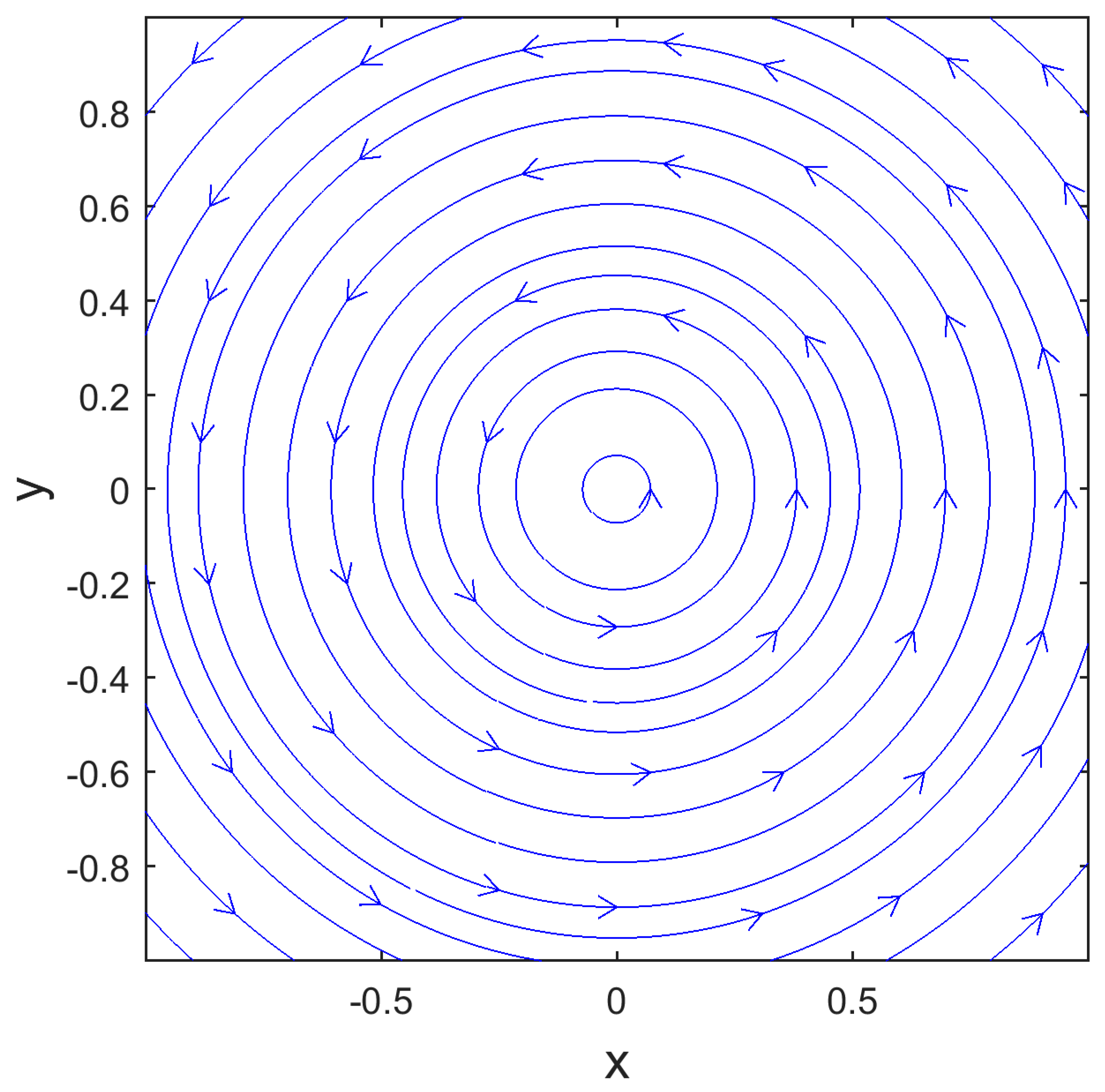
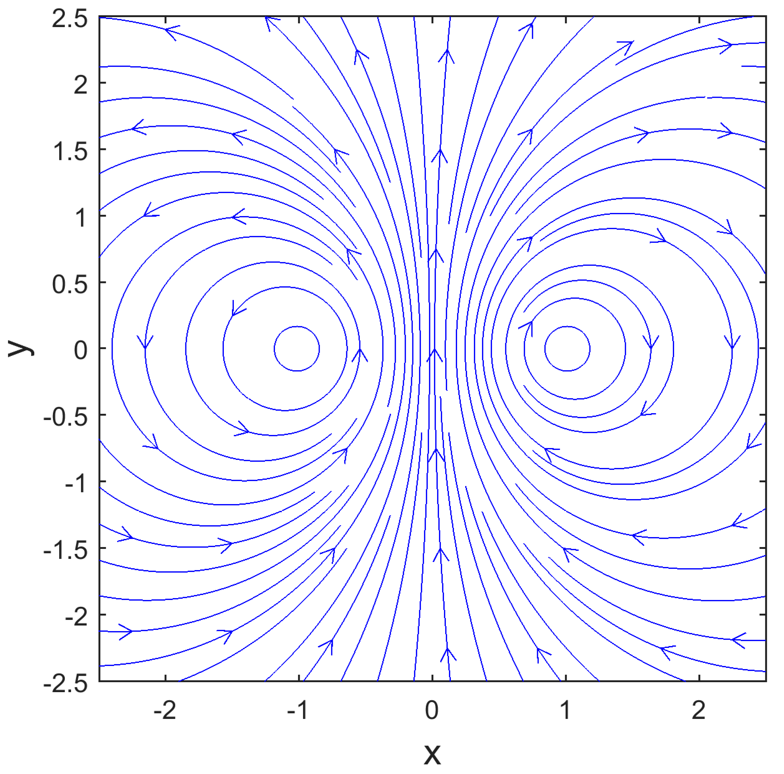
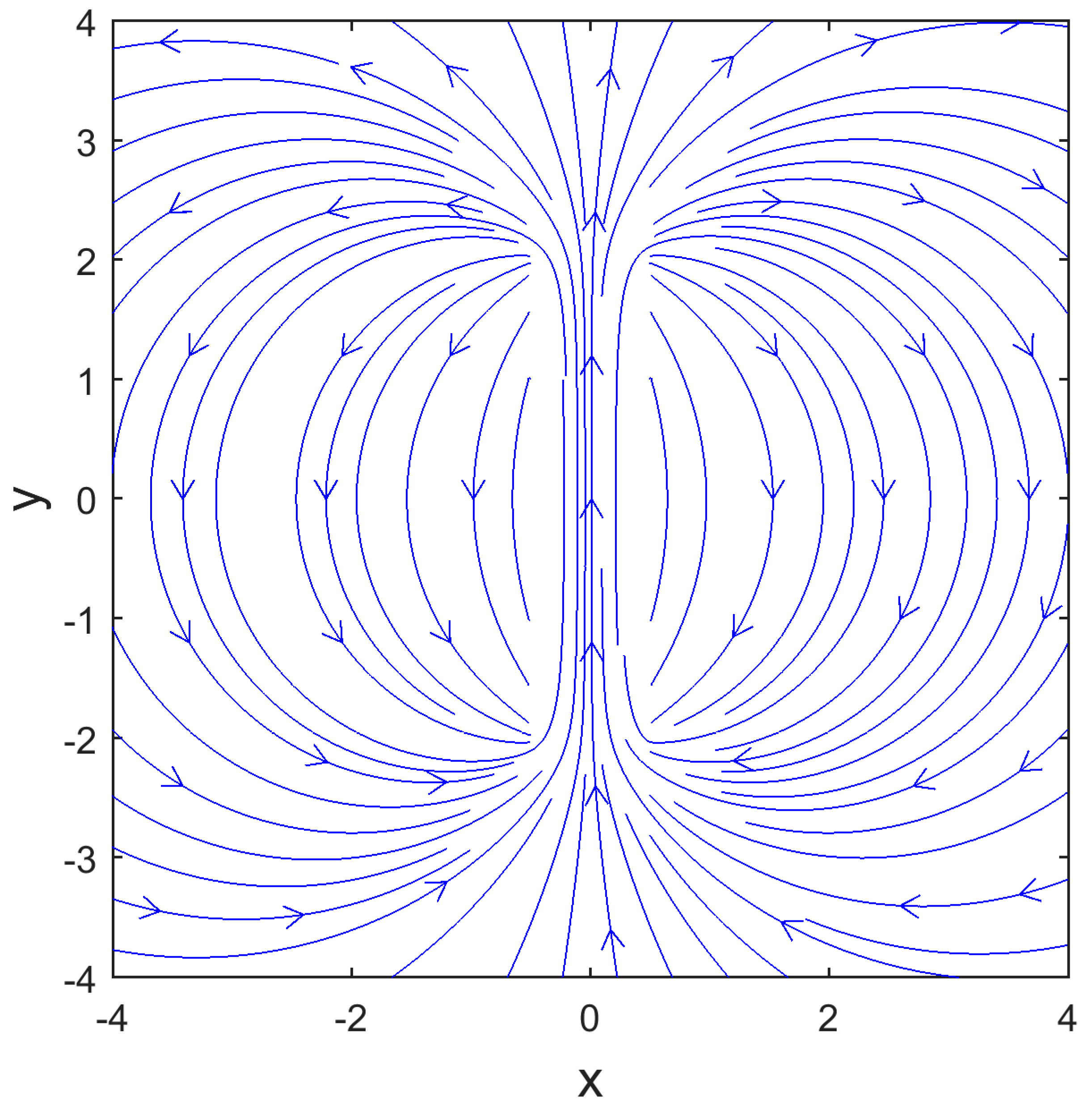
2.1. Laboratory Projects

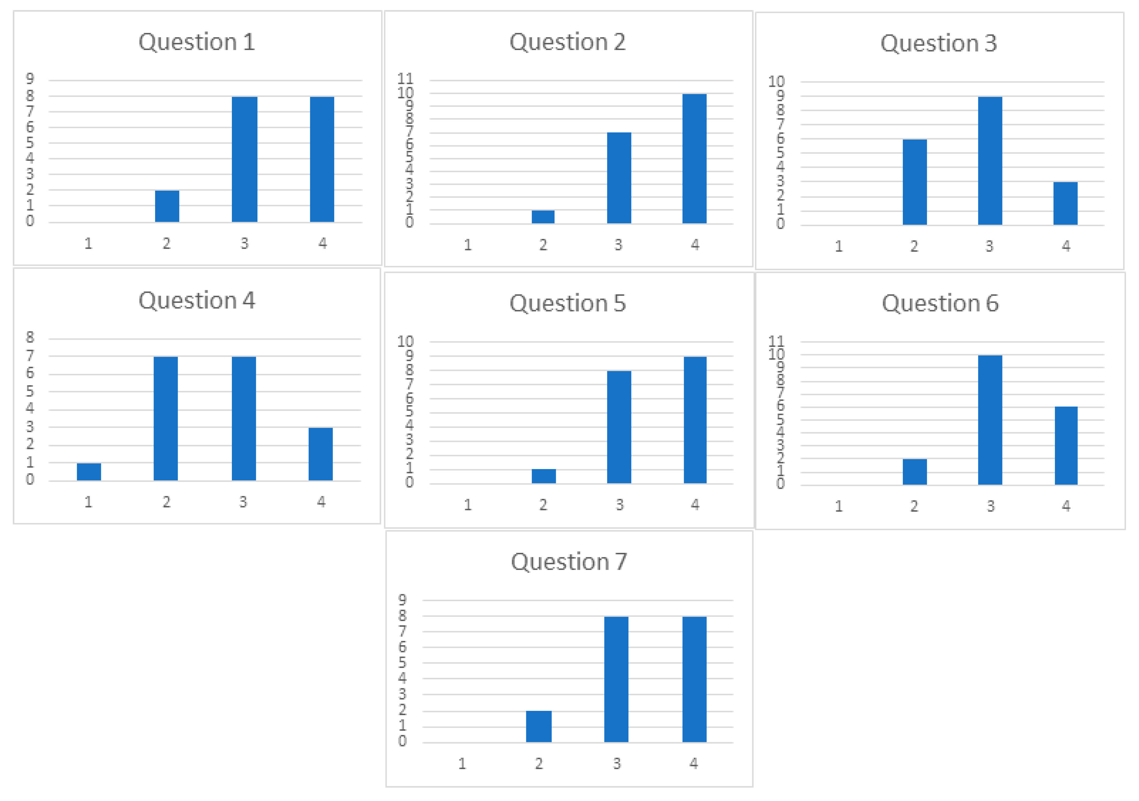
The set of physical situations in Electromagnetism (configurations of electric charges or currents, for instance) that can be studied by the students using pen and paper, in a few minutes, is reduced. The use of programming environments such as MATLAB^® or OCTAVE extends this set of situations allowing computational calculations that without the use of these tools would be slow and repetitive, and thus allowing students to deepen their understanding of more complex problems. OCTAVE (which is open source) is indeed a very good alternative to MATLAB® in the teaching of many laboratory teaching projects in Physics. However, the specific teaching projects presented in this paper need commands which are not yet available in OCTAVE (such as ‘streamslice’).

The first project that we have described is related to the question of the electric field usually assigned to students of Electromagnetism: how to determine the electric field created by a set of point charges?

Theoretically, the electric field of a point charge distribution (e.g., Figure 1) is the superposition of the fields created by each of the charges, and it is given by [14]:

$$\overrightarrow{E}=\frac{1}{4\pi {\epsilon }_0}{\displaystyle \sum _{i=1}^N}\frac{q_i}{r_i^2}{\widehat{r}}_i$$

(1)

where q_i is the value of the charge i (including the sign), r_i is the distance between the charge i and the point where the field is determined, $\widehat{r_i}$ the unit vector pointing from the charge i to that point (for a single charge, it will point from a positive charge to infinity or from infinity to a negative charge), and 1/(4πε₀) a constant (with value 8.99 × 10⁹ N·m²/C² in SI units).

The students attend to the application of this principle in theoretical classes and are encouraged to solve several exercises typically with two (or three) point charges before the theoretical-practical class (in which they can check their results or watch again the application of the general principle). However, these exercises generally only allow the electric field to be calculated at specific points in space, which greatly limits the comprehension of the electric field. Although graphing the electric field generated in all space is trivial for a single point charge, the degree of difficulty increases disproportionately for systems with two or more charges. To obtain the electric field at all points of space, or drawing the lines of it, requires more effort from the students, when the tools used are paper and pen. On the contrary, in laboratory classes, students can obtain representations of the electric field in a systematic way and for any finite distribution of point charges if they are challenged to elaborate computational routines in MATLAB®. In their simplest formulation, these routines begin by creating a grid of equally spaced points on a plane (x,y), and then calculate the electric potential at the points of that grid, having previously been given a distribution of charges q_i in points (x_i,y_i) [14]:

$$V=\frac{1}{4\pi {\epsilon }_0}{\displaystyle \sum _{i=1}^N}\frac{q_i}{\sqrt{{\left(x-x_i\right)}^2+{\left(y-y_i\right)}^2}}$$

(2)

Then, it is enough to use equation

$$\overrightarrow{E}=-\overrightarrow{\nabla }\mathrm{V}$$

(3)

to obtain the electric field. The visual result is that of Figure 2 for an electric dipole (two charges of equal modulus but opposite sign) and Figure 3 for an electric quadrupole (four charges of equal modulus but opposite sign). Both equipotential lines and electric field lines are included. Students are led to consider other charge distributions by always obtaining field lines and equipotential lines.

Afterwards, students are challenged to adapt the previous design in order to obtain (in a plane) the electric field of a parallel plate capacitor (Figure 4), placing two rows of charges with opposite signs aligned face to face, which allows to illustrate the superposition principle in a powerful way: a sum of electric dipoles (with charges of the same modulus and at the same distance) approximates in the plane the field of a capacitor, one of the most important circuit elements.

It must be noted that by changing the linear dimensions of the distribution, students are able to perceive the changes in the field that are obtained with different relations between the width of the plates of a capacitor and the distance between them.

The second project, which we will now describe, focuses on the question of the determination of the magnetic field created by a set of filiform electric currents (e.g., Figure 5 and Figure 6). The answer to this question is trivial for a single filiform current: theoretically, the resulting magnetic field is obtained from Ampère’s Law and it is given (in cylindrical coordinates) by [14]:

$$\overrightarrow{B}=\frac{{\mu }_{0}I}{2\pi r}\widehat{\theta }$$

(4)

In which r is the distance from the current that creates the field to the point where the field is determined, $\widehat{\theta }$ is the unit vector that indicates the direction of any circle centered on the current, I is the current that generates the field and μ₀ is the magnetic permeability of the vacuum (which has the value 4π × 10⁻⁷ H/m in SI units).

Students apply Ampère’s Law in a reduced set of situations in theoretical-practical classes, since there are not many situations for which the determination of the magnetic field is attainable with pen and paper. In laboratory classes one can expand these possibilities and develop the student’s intuition of the magnetic field. Specifically, if we have two electrical currents with opposite directions, with the same intensity, that intersect perpendicularly a plane (x,y) in positions (x′,y′), the magnetic field generated by each current in this plane (in cartesian coordinates) will be [14]

$$\overrightarrow{B}\left(x,y\right)=\frac{{\mu }_{0}I}{2\pi }\left[\frac{y^{\prime }-y}{{\left(x-x^{\prime }\right)}^2+{\left(y-y^{\prime }\right)}^2}\widehat{i}+\frac{x-x^{\prime }}{{\left(x-x^{\prime }\right)}^2+{\left(y-y^{\prime }\right)}^2}\widehat{j}\right]$$

(5)

The visual result for two currents with (x′,y′) = (±1.0) is that of Figure 6, and corresponds to the magnetic field generated by a circular loop placed in the plane (x,z) (computationally, one possible embodiment is to generate a grid of points (x,y) in a region that includes the currents and then calculating the two components B_x and B_y of the field).

As in the previous problem, students are challenged to adapt the protocol to obtain the magnetic field of a rectilinear solenoid by placing two rows of oppositely aligned chains of opposite directions, illustrating once more the superposition principle and showing as the magnetic field of a set of very close turns approximates the field of a solenoid (an important circuit element) in the plane (Figure 7).

Also, in this case, changing the linear dimensions allows the student to observe the differences in field lines for different relationships between the length of the solenoid and its radius.

2.2. Questionnaires

To evaluate the students’ opinions, a questionnaire was used in which we asked students to rate seven questions on a Likert scale from 1 to 4 (1—I do not agree at all, 2—I do not agree, 3—I agree, 4—I totally agree). The total number of students who answered this questionnaire was 18 (16 males and 2 females). Eleven were Portuguese, six from Angola and one from Brazil. There were 24 students in this course (Electromagnetism I), 5 left it early in the semester, 18 out of the remaining 19 answered the questionnaire, 10 were approved, all of which were in the group of 18 who answered the questionnaire. The approved students had an average grade of 15.7 (out of 20) in the laboratory, and 13.3 (out of 20) in the written evaluation. So, besides enhancing the student’s apprehension of the notion of field, the students also have a motivation to attend laboratory classes as the laboratory grade improves the final grade (30%).

The neutral response hypothesis was not given. In this questionnaire we sought in the first question to gauge the level of difficulty felt by the student in relation to the course, in the second we wanted to know if the students understood the importance of programming in their subject of study, with the third and fourth questions we evaluated the level of students’ difficulty with programming (in particular with MATLAB®), and finally with the last three we wanted to know if the activities developed were useful to them. Thus, the questions posed to the students were the following:

• Electromagnetism is a difficult subject in my degree.
• Computer programming is a useful tool for my future work.
• is an accessible learning tool.
• The programming concepts presented in the activities developed in the practical classes are simple and easy to use.
• The graphical interfaces used allow one to easily view field lines, either scalar or vector.
• Using the computational programming activities was useful to simulate physical situations that I could not visualize in the theoretical classes.
• Computer programming activities allowed me to have a better understanding of the concept of field.

The results obtained are represented in the bar charts presented in Figure 8. Regarding the questions asked, we calculated the percentage of students that agree or totally agree with the statement, and we calculated the average of the levels in order to have a notion of the deviation from the mean value of the scale, 2.5 (we also indicate the most frequent value—mode): in question 1—89%, average 3.3 and modes 3 and 4; in question 2—94%, mean 3.5 and mode 4; in the question 3—67%, average 2.8 and mode 3; in question 4—56%, mean 2.7 and modes 2 and 3; in the question 5—94%, mean 3.4 and mode 4; in question 6—89%, mean 3.2 and mode 3; in question 7—89%, average 3.3 and modes 3 and 4. With the exception of questions 3 and 4, they all show a significant agreement with the statement presented.

3. Final Remarks

Two of the problems presented to us in the teaching of electromagnetism are that of transmitting the concept of field (electric and magnetic) and explaining why the linear dimensions of certain components (capacitors and solenoids) of theoretical view, as if they were infinite. In this sense, the two laboratory projects that we presented sought to be a cognitive support for the students, as mentioned by Azmi et al. [15]. From the analysis of the questionnaires, the answers to the last three questions, suggest that the computational programming is, in the opinion of the students, a good strategy to overcome the difficulties described above as expected [11,12]. This positive aspect of programming strategies is more pronounced in the question of understanding the notion of field given the mode and the mean deviation we obtained in questions 5 and 7. Questions three and four do, however, reflect a significant number of students, with some resistance to programming, although they are students of the 2nd year, already with a programming discipline (in C ++). This difficulty is usually felt in this type of approach [13], but it has not been a sufficiently strong obstacle that has prevented students from being able to carry out the proposed tasks. The answers to the first question give us the indication that this course is considered difficult, which makes us consider important the use of diversified strategies that deviate from the traditional teaching of the subject, as suggested by Heeg et al. [16]. Regarding the answers to the second question, we find that they have a strong majority opinion of the importance of programming for the continuation of their studies.

We also acknowledge that a current limitation of this study is the number of students that were involved in the questionnaire, despite the efforts of the authors to receive more data. As an upcoming study, we are planning further studies involving more students.

As future work, we intend to further develop the line of research followed so far by gauging the student´s grasp of the approximations made in both the electric field of finite capacitors and the magnetic field of finite solenoids, as compared to their infinite counterparts.

References

1. Papert, S. Mindstorms: Children, Computers, and Powerful Ideas; Basic Books: New York, NY, USA, 1980. [Google Scholar]
2. Teodoro, V. Modellus: Learning Physics with Mathematical Modelling. Ph.D. Thesis, FCT—Universidade Nova Lisboa, Almada, Portugal, 2002. [Google Scholar]
3. Lopez, S.; Veit, E.; Araujo, I. Una revisión de literatura sobre el uso de modelación y simulación computacional para la enseñanza de la física en la educación básica y media. Rev. Bras. Ensino Física 2016, 38, e2401. [Google Scholar] [CrossRef]
4. Neves, R.; Teodoro, V. Enhancing Science and Mathematics Education with Computational Modelling. J. Math. Model. Appl. 2010, 1, 2–15. [Google Scholar]
5. Neves, R.; Teodoro, V. Modelação computacional, ambientes interactivos e o Ensino da Ciência, Tecnologia, Engenharia e Matemática. Rev. Lusófona Educ. 2013, 25, 35–58. [Google Scholar]
6. Carvalho, P.S.; Christian, W.; Belloni, M. Physlets e Open Source Physics para professores e estudantes portugueses. Rev. Lusófona De Educ. 2013, 25, 59–72. [Google Scholar]
7. Silva, S.; da Silva, R.L.; Junior, J.T.G.; Gonçalves, E.; Viana, E.R.; Wyatt, J.B.L. Animation with Algodoo: A simple tool for teaching and learning physics. Exatas 2014, 5, 28. [Google Scholar]
8. Iwaniec, D.; Childers, D.L.; van Lehn, K.; Wiek, A. Studying, Teaching and Applying Sustainability Visions Using Systems Modeling. Sustainability 2014, 6, 452–4469. [Google Scholar] [CrossRef]
9. Heidemann, L.; Araujo, L.; Veit, E. Atividades experimentais com enfoque no processo de modelagem científica: Uma alternativa para a ressignificação das aulas de laboratório em cursos de graduação em física. Rev. Bras. Ensino Físíca 2016, 38, 1504. [Google Scholar] [CrossRef]
10. Neves, R. Melhorar o ensino e a aprendizagem do electromagnetismo com modelação computacional interactiva. Rev. Lusófona Educ. 2017, 35, 171–190. [Google Scholar]
11. Burke, C.J.; Atherton, T.J. Developing a project-based computational physics course grounded in expert practice. Am. J. Phys. 2017, 85, 301–310. [Google Scholar] [CrossRef] [Green Version]
12. Caballero, M.D.; Burk, J.B.; Aiken, J.M.; Thoms, B.D.; Douglas, S.S.; Scanlon, E.M.; Schatz, M.F. Integrating numerical computation into the modeling instruction curriculum. Phys. Teach. 2014, 52, 38–42. [Google Scholar] [CrossRef]
13. Chabay, R.; Sherwood, B. Computational physics in the introductory calculus-based course. Am. J. Phys. 2008, 76, 307–313. [Google Scholar] [CrossRef]
14. Alves, R.G. Introdução ao Electromagnetismo; Edições Universitárias Lusófonas: Lisboa, Portugal, 2005. [Google Scholar]
15. Azmi, N.A.; Mohd-Yusof, K.; Phang, F.A.; Hassan, S.A.H.S. Motivating engineering students to engage in learning computer programming. Adv. Intell. Syst. Comput. 2018, 627, 143–157. [Google Scholar]
16. Heeg, J.J.; Flenar, K.; Ross, J.A.; Okel, T.; Deshpande, T.A.; Bucks, G.; Ossman, K.A. Effective educational methods for teaching assistants in a first-year engineering MATLAB® course. In Proceedings of the 121st ASEE Annual Conference and Exposition: 360 Degrees of Engineering Education, Indianapolis, IN, USA, 15–18 June 2014. [Google Scholar]
Figure 1. Representation of the electric field and the equipotential lines of a single point charge (see Appendix A for code).
Education 09 00064 g001
Figure 2. Representation of the electric field and the equipotential lines of an electric dipole.
Education 09 00064 g002
Figure 3. Representation of the electric field and the equipotential lines of an electric quadrupole.
Education 09 00064 g003
Figure 4. Representation of the electric field and equipotential lines for a parallel plate capacitor.
Education 09 00064 g004
Figure 5. Representation of the magnetic field created by one filiform electric current (see Appendix A for code).
Education 09 00064 g005
Figure 6. Representation of the magnetic field created by two electrical currents with opposite directions.
Education 09 00064 g006
Figure 7. Representation of the magnetic field lines of a solenoid.
Education 09 00064 g007
Figure 8. Bar graphs with frequency distribution on the Likert scale for each of the questions put to students.
Education 09 00064 g008