Article

Optimizing University Admission Processes for Improved Educational Administration Through Feature Selection Algorithms: A Case Study in Engineering Education

1
Industrial Engineering Department, University of Santiago de Chile, Santiago 9170124, Chile
2
Facultad de Ingeniería, Ciencia y Tecnología, Universidad Bernardo O’Higgins, Santiago 8370993, Chile
3
School of Business, Universidad Adolfo Ibáñez, Av. Diagonal Las Torres 2640, Peñalolen, Santiago 7500975, Chile
*
Authors to whom correspondence should be addressed.
Educ. Sci. 2025, 15(3), 326; https://doi.org/10.3390/educsci15030326
Submission received: 12 October 2024 / Revised: 19 February 2025 / Accepted: 28 February 2025 / Published: 6 March 2025
(This article belongs to the Special Issue Advancements in the Governance and Management of Higher Education)

Abstract

:
This study presents an innovative approach to support educational administration, focusing on the optimization of university admission processes using feature selection algorithms. The research addresses the challenges of concept drift, outlier treatment, and the weighting of key factors in admission criteria. The proposed methodology identifies the optimal set of features and assigns weights to the selection criteria that demonstrate the strongest correlation with academic performance, thereby contributing to improved educational management by optimizing decision-making processes. The approach incorporates concept change management and outlier detection in the preprocessing stage while employing multivariate feature selection techniques in the processing stage. Applied to the admission process of engineering students at a public Chilean university, the methodology considers socioeconomic, academic, and demographic variables, with curricular advancement as the objective. The process generated a subset of attributes and an application score with predictive capabilities of 83% and 84%, respectively. The results show a significantly greater association between the application score and academic performance when the methodology’s weights are used, compared to the actual weights. This highlights the increased predictive power by accounting for concept drift, outliers, and shared information between variables.

1. Introduction

Access to university constitutes a problem whose relevance is based on the recognition of higher education as a right, whose access must be equal and based on merit; Furthermore, it represents an opportunity to obtain a better quality of life (United Nations, n.d.). The challenge of accepting without prejudice and with equity and inclusiveness the students who present the best academic performance (AP) at the higher education institution has generated abundant analysis and debate (Al-Okaily et al., 2024).
Poor student selection entails serious consequences at the personal, institutional, and public levels. The admission of a student lacking a vocation can lead to their dropout, resulting in emotional, familial, economic, and occupational impacts (Espinoza et al., 2024b). For higher education institutions it has an obvious economic cost (d’Astous & Shore, 2024), derived from the need for reprocessing and new processes to resolve the lack of skills, as well as the loss of students without vocation; Likewise, it harms its quality and prestige indicators (Espinoza et al., 2024a). At the public level, the cost of dropout impacts government spending, which affects even more the lowest social strata even when higher education enters the universalization phase (Hinojosa, 2021).
The intrinsic complexity of the educational process makes the analysis of this problem challenging (Eshet, 2024). The various inputs and variables that influence the educational process, combined with distinct technologies and control measures, lead to dissimilar outcomes (Fuertes et al., 2015). The student, with all his uniqueness, is influenced by a changing social, institutional, and regulatory environment and, in addition, participates in the process as raw material, product in the process, finished product, process participant, and co-owner of the process (Aguayo-Hernández et al., 2024; Vargas et al., 2019).
Model-based or generative philosophy (Williams, 2021), in which a function is sought to represent the real system, is the one that is mainly used to study this problem. Under this explanatory approach, Yarkoni and Westfall (2017) have measured the importance of variables using linear regression (LR), obtaining multiple well-fitted models, which produces an underdetermination of the theory (Palacios et al., 2021); in addition, the estimation of values based on a single sample generates overfitting (Alalawi et al., 2024) and does not really predict (Hilbert et al., 2021). Another tool that is used is the Pearson coefficient ( r P ), with which the association between variables is measured, but without considering the interaction between them, which does not reflect reality. Both this and LR require that the variables be linearly related and meet certain requirements, which does not adapt to the complexity.
In contrast, under the data-driven philosophy algorithms are constructed (Vargas et al., 2020), not equations, accepting that the underlying process produces data in a black box, whose interior is complex and partially unknown, into which variables enter and from which variables exit (Matsushita, 2024). Algorithmic modeling therefore allows us to predict AP from admission variables, which implies an association between them (Shmueli & Koppius, 2011).
Based on the foregoing, the purpose of this research is to overcome the mentioned limitations through a methodology based on machine learning (ML), which addresses the complexity of the selection process without imposing restrictions on the variables and their relationships, to produce the subset of attributes and weight of selection criteria (SC) best associated with AP.
Following the thinking of John Tukey (Shmueli & Koppius, 2011), two working philosophies are identified: (i) The model-driven approach and (ii) the algorithmic approach. In (i) we seek to represent the real system through a function with parameters to estimate and validate (Shmueli & Koppius, 2011).
Practically all studies employ the same methods and tools. To evaluate the association between variables, pairwise correlation measures are used (Vergara-Díaz & Peredo-López, 2017). The importance of the variables is obtained with simple, multiple, or logistic regression models. Predictability is evaluated both for all cohorts together and separately, and for a unit of analysis that can be a study program, an area of knowledge, or an institution.
However, these methods present several risks. Firstly, the variables may not meet the requirements of independence, normality, and homoscedasticity. Additionally, they tend to minimize bias at the expense of increasing variance, leading to model overfitting to the data (Yarkoni & Westfall, 2017). Finally, arbitrary decision-making can lead to a lack of replicability (Uvidia Fassler et al., 2020), known as p-hacking.
On the other hand, (ii) makes use of ML technologies, which are fundamental in data science and artificial intelligence. Although the use of ML in the field of education is still limited, it is growing in research focused on academic performance (Albreiki et al., 2021). In various university contexts, ML is used with an explanatory approach in admission processes, where the importance of features is determined through Naïve Bayes classifier (Rawal & Lal, 2023), clustering (Harsono et al., 2024), and sensitivity analysis (Marbouti et al., 2021). Moreover, the algorithmic approach does not impose restrictions on the variables, does not presuppose a theoretical function, and can capture complex patterns and relationships (Shmueli & Koppius, 2011), predict with new data, avoiding overfitting and improving reliability, seeks a balance between variance and bias, adjusting the model to maintain generalization (Shmueli & Koppius, 2011) and is more robust against outliers (Hilbert et al., 2021).
Other authors seek subsets of attributes that best predict AP, measuring their importance through feature selection (FS) algorithms (Contreras et al., 2020; Wu & Wu, 2020). They have used filters, wrappers, and embedded algorithms (Venkatesh & Anuradha, 2019). With different methods and strategies, they have achieved precision with decision trees ranging from 28.9% (Putpuek et al., 2018) to 73.3% (Adeyemo & Kuyoro, 2013), and accuracy with neural networks ranging from 80% (Echegaray-Calderon & Barrios-Aranibar, 2016) to 91% (Rachburee & Punlumjeak, 2015). This variability in performance is attributed to differences in context, the technology used, the operationalization of variables, and the quality of the data.

1.1. Contributions and Limitations of the Study

This document contributes to the field of data science applied to educational management through four main contributions.
  • Validation of ML for the analysis of the university admission system.
  • Incorporation of concept drift management and outlier handling in the data preprocessing stage.
  • Establishment of precision as a performance measure for the models.
  • Development of a procedure to determine the weights of selection criteria.
It is important to consider some limitations. The levels of precision, validity, and reliability of the developed models are contingent upon the context and data (variables and their respective distributions) of this study. Therefore, these results may not automatically generalize to other applications or datasets.

1.2. Literature Related to Machine Learning for Optimizing University Selection

This research proposes the inclusion of processes and procedures aimed at increasing the validity and reliability of the analysis. This is achieved by reducing bias in the choice of the dataset, minimizing data distortion, and justifying a performance measure (Velmurugan & Anuradha, 2016). Additionally, a heuristic is added to the feature selection technique to obtain an optimal subset of features, allowing the determination of the weights of key SC in the admission system. Table 1 provides a summary of the most relevant features of the algorithms used in the main studies included in the literature review.

1.2.1. Reducing Bias in Data Selection

In the process of prediction with rectangular data, two implicit assumptions are established about the examples used to train the machine. First, they are assumed to be statistically independent (Gama et al., 2004), meaning that given the training vectors x i X , the condition P ( x j | x k ) = P ( x j ) , j k , holds. This allows for the random selection of samples and preserves the model’s generalization capability. In this research, this assumption is met, as each case corresponds to a different student. The second assumption is that the data are equally distributed (Gama et al., 2004), meaning that the features and the target, X and y , come from the same joint probability distribution P ( X , y ) . However, this stationarity requirement is not guaranteed when operating with a conceptual sample, which can introduce biases and compromise the effectiveness of the generated model (Gama et al., 2004; Hilbert et al., 2021).
The concept, P ( X , y ) , in the presence of dependency is expressed as P ( X , A P ) = P ( X ) · P ( A P | X ) (Zhou et al., 2019). A drift in any of these probabilities generates concept drift (CD). If it arises from a drift in the posterior probability, that is, for two cohorts 1 and 2, P 1 ( A P | X ) P 2 ( A P | X ) , it is called real, as it affects decision-making (Lu et al., 2019; Yang et al., 2020). If the drift is only in P ( X ) , it is called virtual or data drift (Lu et al., 2019; Yang et al., 2020), and does not affect decision boundaries. The change in P ( A P ) is called label drift (LD) or class prior probability shift (Lu et al., 2019). Generally, the CD is classified as a hybrid (Yang et al., 2020).
Depending on how CD occurs over time, four situations may arise (Webb et al., 2016): (i) sudden, if it only occurs from one cohort to another; (ii) gradual, if it occurs with increasing frequency until it becomes definitive; (iii) incremental, if its magnitude progressively increases until a final state; and (iv) recurrent, if it occurs for a while, then returns to the previous state, and this repeats.
Integrating CD into the analysis involves detection, understanding, and adaptation (Lu et al., 2019). For detection, algorithms based on the error rate (Frías-Blanco et al., 2015; Gama et al., 2004; Lu et al., 2019; Xu & Wang, 2017) are the most used (Hashmani et al., 2020; Yang et al., 2020). Another option is to quantify the difference in data distributions (Yang et al., 2020), between a historical time window and a new one (Hashmani et al., 2020; Lu et al., 2019). Another method is domain classification (Deepchecks, 2023), where old data are labeled with 0 and new data with 1, and they are mixed for training; if a learner easily predicts the class, then CD exists (Chorev et al., 2022).
Once detected, it is necessary to understand when, how, and where it occurs. The year t in which it occurs when P t ( X , R A ) P t + 1 ( X , R A ) , which may require a complete or partial model update (Gama et al., 2004). How it occurs means determining the severity of the change ( Δ ) through a discrepancy function δ , such that Δ = δ ( P t ( X , R A ) , P t + 1 ( X , R A ) ) ; with an error rate detector, the degree of precision decrease can be used as a proxy. Lastly, where it occurs corresponds to the areas of the feature space where CD is found.
Regarding adaptation, existing algorithms (Hashmani et al., 2020; Xu & Wang, 2017) focus on CD in data streams due to their unique characteristics (Guo et al., 2021). Stationary data, like the batches produced by the admission process, do not require adaptation algorithms, as all analysis is performed asynchronously, and it is sufficient to detect, understand, and adapt to manage CD.

1.2.2. Measuring Performance in Predictive Models

In the ML domain, there is no single algorithm that is optimal for all contexts (Wainer & Cawley, 2021). Therefore, this study is based on a diverse set of predictive algorithms, including decision trees, naive bayes, support vector machine, neural networks (NN), linear discriminant analysis and quadratic discriminant analysis, k-nearest neighbors (kNN), and logistic regression. The same applies to model fitting and evaluation, where the chosen strategy—whether a holdout sample, k-fold cross-validation (CV), or nested CV—best fits the problem at hand (Wainer & Cawley, 2021).
The validity and reliability of the predictive models obtained with these strategies and algorithms depend on the measurement of their performance. This evaluation is crucial for optimizing the model’s hyperparameters in the validation set and subsequently estimating its performance on an independent test set. Given the importance of this, the selection of the appropriate performance indicator must be performed carefully and prior to the modeling stage.
In this study, precision is considered the primary indicator, as false positives are associated with higher costs in the context of the problem addressed (Hilbert et al., 2021). For multiclass AP, the weighted average of class precisions, p w , and the unified precision of all classes, p m , are used. If not specified, it corresponds to the dichotomous case, p , and if it is in training, p T .

1.2.3. Distortion Due to Outliers

There is no standardized mathematical definition of an outlier, which requires an interpretation adapted to the problem domain. Evidently, poorly recorded data generate outliers, but they can also arise from students who lack the vocation or competencies to study a particular career, as their learning process does not align in the same way as an individual for whom the program was designed. Therefore, these cases should be discarded, especially considering that there are algorithms sensitive to outliers, such as decision trees.
An indirect way to identify these students is through dropout statistics (Deepika & Sathyanarayana, 2022), considering that not all under this condition necessarily drop out. According to a study applied in the admission system (Mineduc, 2008), of the total students who drop out, 30% do so due to vocational factors, 20% due to economic reasons, 19% due to poor academic performance, 17% due to unmet expectations, and 14% due to insufficient pre-university competencies. If vocation represents at least 30%, plus an unknown part of the 19% and 17%, a maximum of 66% is deduced; and if competencies represent at least 14%, plus an unknown part of the 19%, a maximum of 33% is produced.
Various algorithms are used to detect outliers: probabilistic ones like ABOD and KDE; linear ones like PCA, KPCA, and OCSVM; proximity-based ones like kNN, AvgkNN, LOF, CBLOF, and HBOS; ensemble-based ones like IF; and neural network-based ones like MOGAAL and ALAD (Zhao et al., 2019). When evaluating without the outliers, the goal is to improve the model’s performance.

1.2.4. Feature Selection in Knowledge Mining

FS is employed to identify an optimal subset of features relevant to the problem (Affendey et al., 2010). Additionally, a heuristic based on FS is proposed to obtain the weighting of SC. Given the absence of a universal algorithm for FS, various methods classified into three categories are considered: filters, wrappers, and embedded methods (Pilnenskiy & Smetannikov, 2020).
The filter mutual information maximization (MIM), with its univariate relevance criterion, allows assigning a score to each feature according to the maximum mutual information between it and the academic performance. Given the feature X k and the AP, the mutual information is defined based on Shannon entropy, H , as I ( X k , A P ) = H ( X k ) + H ( A P ) H ( X k , A P ) (Wang et al., 2021), representing the amount of information provided by X k that reduces the uncertainty of the AP.
It is important to consider the interdependence between the features, as it can be either useful (complementarity) or not (redundancy). Various techniques have been developed to determine redundancy and/or complementarity, which compare each candidate feature to the optimal subset, X k , with each preselected feature X S (Wan et al., 2022). Regardless of this definition, the following multivariate filters, whose common theoretical basis is mutual information, are considered: joint mutual information (JMI) (Yang & Moody, 1999), conditional mutual information (CMIM) (Fleuret, 2004), dynamic change in selected feature (DCSF) (Gao et al., 2018a), mutual information based feature selection (MIFS) (Battiti, 1994), conditional infomax feature extraction (CIFE) (Lin & Tang, 2006), minimal redundancy maximal relevance (mRMR) (Peng et al., 2005), composition of feature relevancy (CFR) (Gao et al., 2018b), maximal relevance and maximal independence (MRI) (Wang et al., 2017) and interaction weight-based feature selection (IWFS) (Zeng et al., 2015).
Given that multivariable filters require a preselected feature to calculate redundancy and complementarity, the DCSF, CFR, and IWFS algorithms do not produce a result unless a preselected feature is provided. Meanwhile, the JMI, CMIM, MIFS, CIFE, mRMR, and MRI algorithms generate the same score as MIM (Github, 2024).
In wrapper algorithms, the selection process involves a specific classification model, whose predictive performance is used to evaluate the relative utility of variable subsets. If Q is the measure of model quality, then, given a subset F , the optimal subset F *   is   sought   such   that   F * = a r g m a x [ Q ( F ) ] (Pilnenskiy & Smetannikov, 2020).
Its implementation involves defining, in addition to the classifier and performance indicator, the search strategy. Two of the most used strategies are exhaustive search and greedy search (Cunningham & Delany, 2021). In the former, all possible subsets with m features, 2 m 1 are evaluated. If m is very large, this generates high computational costs and a risk of overfitting (Li et al., 2017). The greedy strategy consists of sequential forward selection or sequential backward elimination (Cunningham & Delany, 2021). For greater flexibility, there is a floating search, which reconsiders already selected or eliminated attributes (Jeong et al., 2015), among other methods (Abdel-Basset et al., 2021; Amini & Hu, 2021). Greedy sequential floating algorithms are chosen for their lower propensity to overfit and flexibility.
Finally, embedded algorithms are considered, in which the remaining features are a byproduct of the modeling process. Among the most used are tree-based methods; the permutation importance method, which measures the impact on prediction by shuffling the data of each attribute; and regularization methods, which minimize fitting errors while forcing the coefficients to be small, such as Lasso and Ridge linear regression (Amini & Hu, 2021; Huang, 2015).
The rest of this document is organized as follows: Section 2 presents a general description of the case study, accompanied by the methodology used in this study, offering a detailed account of each of the steps that make up the model. Section 3 presents the case study results. Section 4 discusses the results obtained. Finally, Section 5 concludes this work and describes some future research topics.

2. Methodology

The case study considers a public university and a target population of applicants/students in engineering programs. The application process is conducted with an application score (PJEPOST), corresponding to the weighting of five criteria: three admission tests (PSUMAT, PSUCIE, PSULYC) and two indicators of academic performance, NEM and RANK, which represent the average grades of the last four years of high school and the ranking relative to the average of the graduating educational institution, respectively. The institution sets the weights and minimum required application scores within regulated ranges (DEMRE, 2022). Based on these decisions, the applicant is either rejected or accepted depending on their PJEPOST rank among candidates for their preferred study program.
The existence and accessibility of data determine the variables to be used. These include 22 input features, among SC and various demographic (DE), socioeconomic (SE), and academic (AC) backgrounds of the applicants. The target, AP, is the percentage of curricular progress (Table 2).
The methodology is structured in the preprocessing and processing stages. Figure 1 outlines the proposed processes for optimizing university admissions. The remaining processes are standard techniques common to any data analysis methodology.

2.1. Preprocessing Stage

This phase begins with (1) the arrangement of the data in the work environment, with the aim of integrating them into an ordered and readable matrix for the computer system to be used.
The second process is (2) data cleaning, whose objective is to reduce noise. In this process, all cleaning is performed, except for the management of missing data in non-key variables (different from SC), since, in the case of SC, missing data are not acceptable. The sample space is checked to identify out-of-range, misleading, and meaningless values, missing values are identified, and cleaning is performed according to the obtained results.
Next, (3) exploratory data analysis (EDA) is performed, with the initial purpose of inspecting the quality and statistical properties of the raw variables. At the end of this stage, another EDA (8) is carried out to confirm the properties of the dataset entering the processing phase; this includes verifying normality in SC, correlation between features and AP, and evaluating the quality of the obtained dataset.
Then, (4) the missing data management process aims to eliminate missing data in variables that are not SC by imputation or elimination
In the following process, (5) feature engineering is performed, which means making the variables operational by transforming them into formats suitable for ML technology. This involves transforming, discretizing, encoding, standardizing, and/or scaling variables.

2.1.1. Concept Drift Management

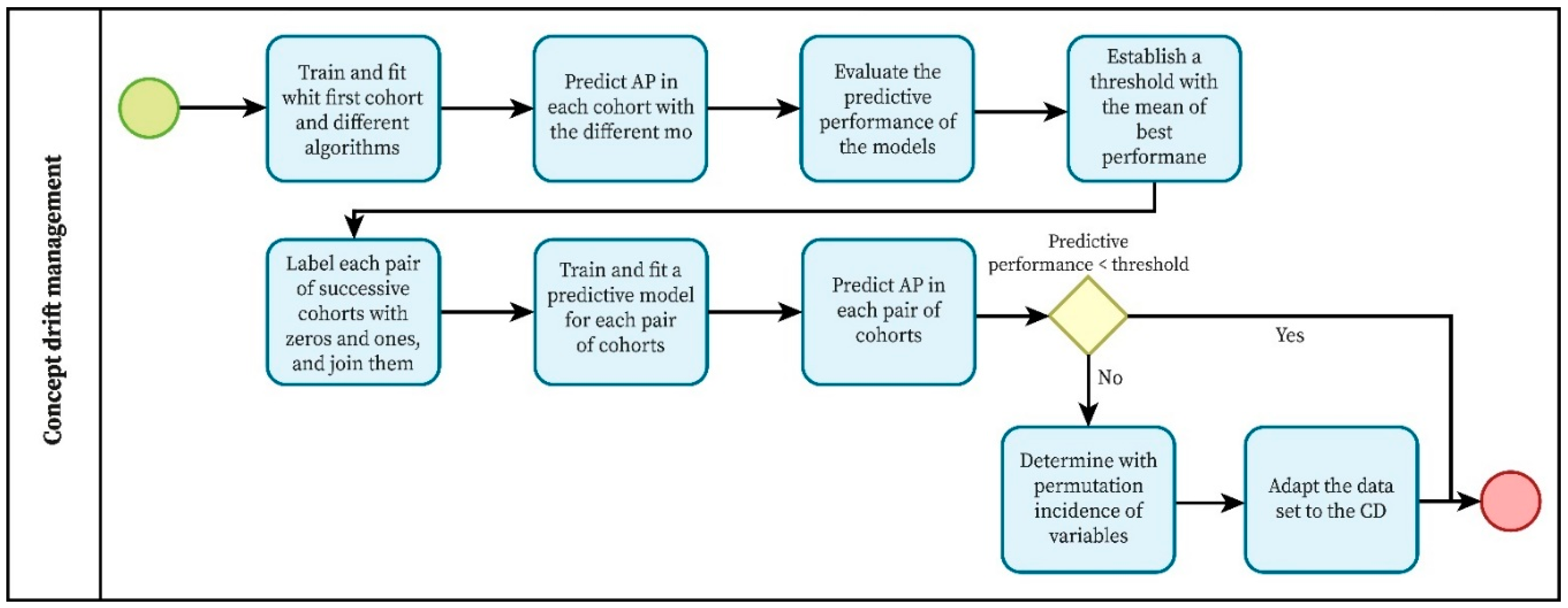
This is a key process, aimed at managing CD (Figure 2). First, CD is detected using domain classification, for example, with a histogram-based gradient boosting tree (HBGB) (Chorev et al., 2022). The threshold or maximum performance level required from this result is determined as the average of the best performances obtained when predicting each cohort with a model trained using the first cohort. Once detected, permutation is applied to determine which variables most influence the CD. With this information and the time at which it occurs, the CD is characterized. Finally, a decision is made on how to adapt the dataset to the CD. The technology used includes encoders, scalers, prediction algorithms, domain classifiers, performance indicators (precision and AUC-ROC), statistics, and graphical tools. AUC-ROC is also used, focusing on the positive class, as it complements precision with a more global perspective. In this, as in the other processes, models are always created with algorithms, strategies, and structures that yield the best performance.

2.1.2. Outlier Management

The objective of this process is to eliminate outliers (Figure 3), To identify them, detection algorithms using different approaches are employed, to which the magnitude of contamination is provided, yielding outlier scores for each instance. A predictive model is then fed with both sets, with and without outliers, and its performance is measured. Next, for each cohort algorithm, the difference in performance with and without outliers is calculated. Finally, the outliers correspond to those identified by the algorithm that produces the greatest difference. The technology used includes scatter plots, distribution plots, regression, histogram, kernel density estimation, and box-and-whisker plots; probabilistic, proximity-based, linear, ensemble-based, and neural network outlier detectors; data frame and file managers; and encoders, scalers, and prediction algorithms.

2.2. Processing Stage

In this stage, knowledge mining is performed.

2.2.1. Feature Subset Search

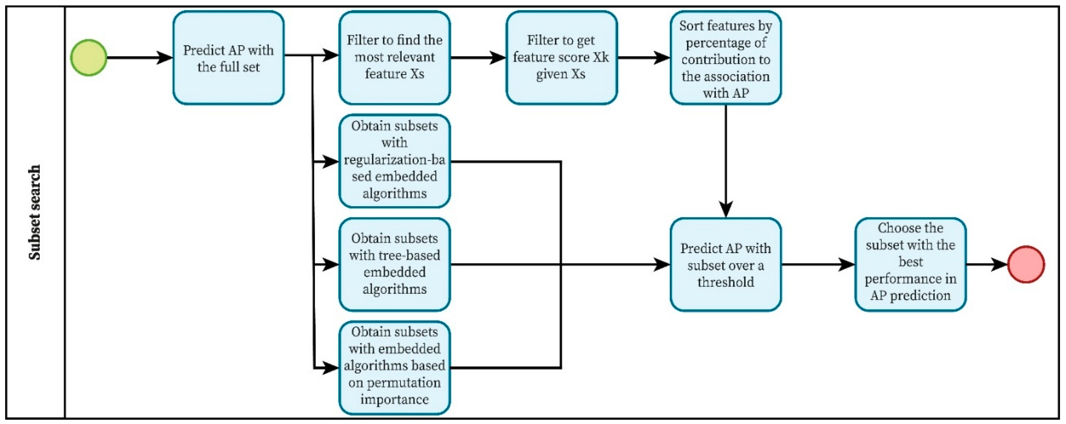
The objective of this process is to obtain the optimal subset of features (Figure 4). Two strategies are executed: filtering and embedded algorithms. The latter, by their nature, automatically provide the subsets. For filters, it is necessary to define a procedure, which begins by running the filters to find the most relevant feature X s . With this feature preselected, the other features are obtained. Then, the attributes are ranked according to their contribution percentage to the association with academic performance, given X s . Feature subsets are defined starting from a cutoff point, defined as a percentage of the explanation of the target given these features. Finally, the feature subset that generates the highest precision in predicting AP with a prediction model trained with the obtained subsets is determined. The technology used includes encoders, scalers, prediction algorithms, performance indicators (precision), association measures, univariate and multivariate filters, and embedded algorithms.

2.2.2. Search for the Selection Criteria Weight

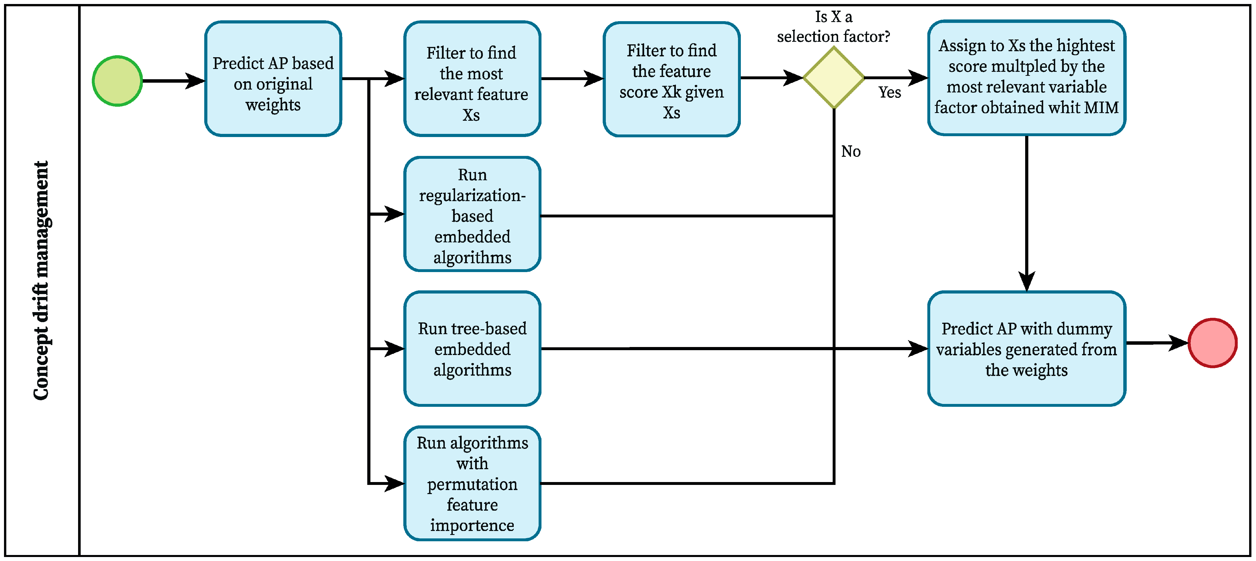
The objective of this process is to obtain the optimal weighting of SC (Figure 5). Two strategies are used: filters and embedded algorithms. The latter, by their nature, automatically provide scores associated with the features; this happens with regularization algorithms and tree-based algorithms. For filters, it is necessary to define a procedure, which begins by running the filters to find the most relevant feature X s . With this feature preselected, the other features are obtained. If X s is a selection criterion and the filter does not generate a score without a preselected variable, the MIM filter is executed, and a “most relevant variable factor” is calculated as the ratio between the two highest scores obtained. Then, the highest-ranking score multiplied by this factor is assigned to X s . With the obtained criteria weights, a fictitious variable for application score (PJEPOST_1) is generated, which feeds a model to predict AP. Finally, the SC ranking that generates the highest precision is selected. The technology used includes encoders, scalers, prediction algorithms, performance indicators, association measures, univariate and multivariate filters, and embedded algorithms.

3. Results

3.1. Preprocessing

The process uses data from 2014 to 2018, collected in an Excel workbook containing 6985 cases and 23 variables. Using the Anaconda 2.4.0 platform (Anaconda, 2024) work is performed in the Jupyter 3.6.3 environment (Granger & Perez, 2021), configured to program and work with files in Python 3.9.16 (Van Rossum & Drake, 2003) and libraries are imported. The 7 demographic variables, 10 academic variables, and 6 socioeconomic variables are organized into a data frame.
In the cleaning process, 82 instances with out-of-range data in key variables and 223 instances with duplicate data are removed. Additionally, the characteristics DE_REGION, SE_ESTADEP, and SE_ESTADIF are removed due to having more than 70% missing data, and DE_NAC is removed due to a significant imbalance in its two categories (6952 Chileans and 33 foreigners). The resulting matrix is 6200 × 19.
In the initial EDA, a length-width ratio of 344:1 is observed. Analyzing the distribution of AP using instance count, histogram, and Kernel density estimation (Pan et al., 2022), it is decided to discretize it, as it takes only 50 distinct values, and its distribution is not homogeneous. This same analysis reveals a certain normality in SC, except for RANK.
For handling missing data in non-key variables, the defined procedure is executed. Random forests (RF) with Bootstrap resampling, NN, support vector machine, and kNN are used. The model is adjusted with stratified cross-validation (to avoid imbalance) five times, shuffling samples before splitting, and with grid search. Since the performances were below 50%, it was decided to discard a variable.
The feature engineering process begins with the discretization of variables. For AP, six performance levels are defined according to the context, and hierarchical alphabetical labels are assigned (Table 3).
Then, preprocessors are defined for scaling and attribute encoding (one-hot for nominal and integer for ordinal) that are executed when models need to be adjusted, as this involves frequent random sampling of data for training the machine and evaluating models.
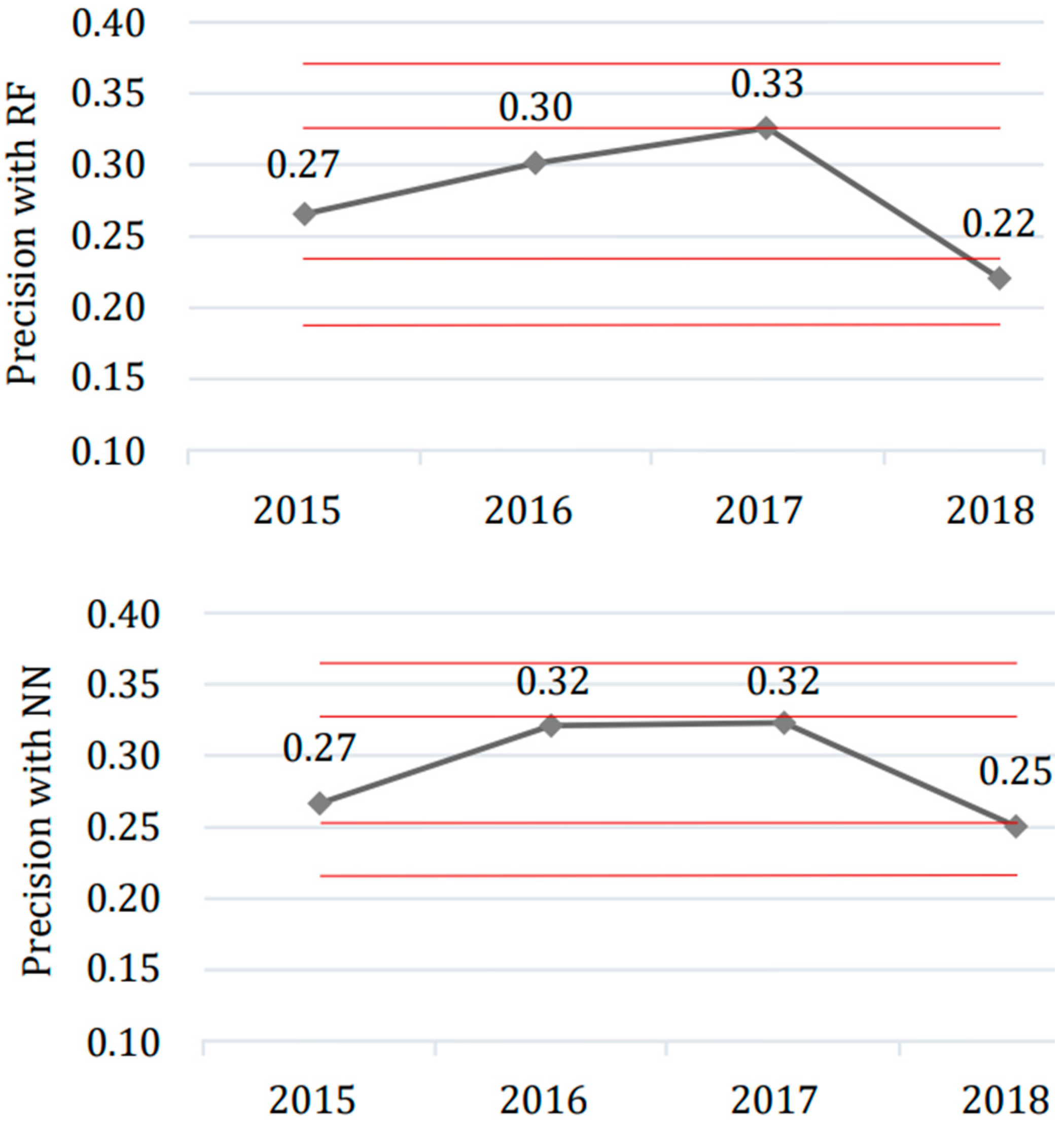
For the CD management process, a matrix of 4958 cases and 16 attributes is used. For the first strategy of the detection procedure, the machine is trained using different algorithms with 2014 data and an 80% stratified reserved sample, with three iterations in stratified cross-validation with grid search. The best performance is obtained with RF and NN (Figure 6), observing a decrease greater than 1 standard deviation (s) in 2018. With the average of the mean performances of the top four models, a threshold of AUC-ROC = 0.63 (s = 0.009) is obtained.
For the second strategy, training-test pairs are set up for 2014–2015, 2015–2016, 2016–2017, and 2017–2018, and are trained with the HBGB tree. For the domain classification strategy, an HBGB predictive model is trained and evaluated on each pair of consecutive cohorts (year, year + 1). For example, the data from 2017 are labeled as zeros, and those from 2018 as ones. With the obtained threshold, the domain classifier model requires a drift value of D V = 2 A U C R O C 1 < 0.26 ; if it is greater or equal, it would imply the existence of a CD. Table 4 shows the scores and the variables that most contributed to not meeting the condition, which together explain more than 80%, obtained through permutation importance measurement. The condition is not met between the 2015 and 2016 cohorts, but since it is at the threshold of the interval and within the margin of error (s), it is not considered. However, between 2017 and 2018, it is evident that a different situation arises. A drift value of 0.73 indicates that there would be a CD, a result consistent with the previous method. Additionally, it is observed that ESTUPAD is the only variable responsible for this change.
To further characterize, an analysis was conducted to determine whether the drift was in features, labels, or only predictions. A slight value above the threshold was found for DECIL in 2017 (0.26) and a significant magnitude for ESTUPAD from 2018 onward (0.59). This feature drift explains the real CD found. Therefore, the 2018 cohort is discarded.
To manage outliers, the information from Section 1.2.3 is applied to the dropout data from 2014 to 2017 (Table 5), obtaining minimum and maximum dropout rates.
Following the defined procedure, 13 outlier detection algorithms are executed for each cohort and percentage (Zhao et al., 2019), using different approaches, obtaining 104 outliers with their associated scores.
The difference in the mean absolute error of RF and NN predictors is calculated, both with and without outliers. The algorithm with the best performance is chosen for each cohort, resulting from the operation with the minimum or maximum percentage (Figure 7); in the case of equal scores, the algorithm with the best average performance is chosen. Figure 7 shows, for example, how the mean absolute error decreased when predicting for the 2015 cohort by removing outliers through the execution of the different algorithms. The selected algorithms are IF for the years 2014, 2015, and 2017, and KDE for 2016, identifying 148, 100, 217, and 165 outliers, respectively. Since the differences in error are small, it is required that an instance be considered an outlier in at least half of the algorithms. Thus, 49, 23, 147 and 60 outliers are obtained, respectively.
To validate the process, the performance of an RF model in prediction is compared, with and without outliers, verifying a slight improvement from 33% to 35% after the removal of these values.
In the final EDA, the non-normality of RANK and RA is confirmed. In addition, the following significant results of univariate correlation between quantitative features and AP are obtained: PSUMAT = 0.49, PSUCIE = 0.41, PSULYC = 0.19, RANK = −0.12. PJEPOST = 0.24; it is not possible to generate any inference from NEM alone. On the other hand, among SC, the natural correlation between RANK and NEM (0.84) is ratified, and the high correlation between PSUMAT and PSUCIE (0.66) and the negative relationship (<=0.4) between all tests and NEM or RANK stand out.
The correlation between AP and socioeconomic and demographic characteristics generates only one significant result greater than or equal to 0.1, r D E C I L R A = 0.1 . With respect to the correlation between categorical features, the only two values in that range are Kendall’s Tau τ = 0.61 (p-value = 0) between ESTUPAD and PRIGE, and a Cramer’s coefficient V = 0.32 between GENE and CARR.

3.2. Processing

The process begins with a matrix of 3828 × 15, consisting of: AP, PSUMAT, PSULYC, PSUCIE, NEM, RANK, DEPA, CARR, PREFPOST, DECIL, ESTUPAD, PRIGE, ANTEGRE, GENE, and TAMFAM. Additionally, PJEPOST is considered, but only for validation procedures.

3.2.1. Prediction Without Feature Selection

In the operation without FS, a stratified sample of 20% is randomly reserved, and an MLP neural network is designed within a stratified CV system, with hyperparameter tuning via grid search. The machine is fed with different sets, each with its respective preprocessing path. The obtained model consists of 14 input neurons, 1 output neuron, and two hidden layers, each containing 4 neurons. It uses the stochastic weight optimization method, Adam, with a regularization coefficient of 0.1. With the final matrix, precision for multiclass AP is obtained at p w = 33.2 % ( p T = 30.7 % ) and for dichotomous AP, p = 79.1 % ( p T = 79.2 % ) (focused on “Pass”). Thus, multiclass AP is discarded.

3.2.2. Optimal Feature Subset

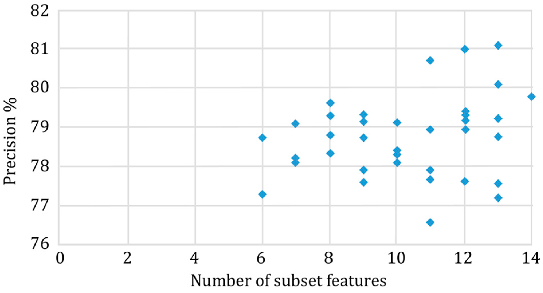
In this procedure, MIFS and mRMR are executed, considering redundancy in addition to relevance calculated with MIM, and CIFE, DCSF, CFR, MRI, DISR, JMI, CMIM, and IWFS that add complementarity. With MIFS, it is necessary to assign a sensitivity value to redundancy (Beta), for which a sweep is performed until the solution stabilizes, which occurs for 1.8 < Beta < 2.5; results that are equivalent to mRMR. The machine is trained with a multi-layer perceptron NN, with stratified CV, adjusted based on a grid of hyperparameters, and its precision in predicting ‘Pass’ is measured (Figure 8). Thus, 27 subsets are obtained with filters, over a 95% explanation percentage. The wrapper strategy is not used as it is not possible to estimate the importance of the original features from the dummy variables produced by one-hot encoding processes. Finally, with embedded algorithms, 11 subsets are found above the threshold, executing permutation on features and impurity measurement by entropy with RF.
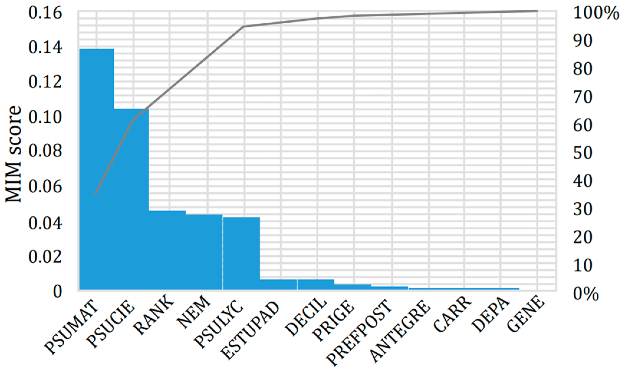
To compare the two best subsets, NN algorithms are executed. The best model, with Adam optimization, a regularization coefficient of 1 × 10⁻⁶, the same number of neurons as input features, 1 output neuron, and two hidden layers of 4 and 3 neurons, respectively, achieves an accuracy of 82.5% ( p T = 79.0 % ) with the MIM filter subset, S M I M 99.6 = {FFSS, ESTUPAD, DECIL, PRIGE, PREFPOST, ANTEGRE, CARR, DEPA, GENE} (Figure 9), equivalent to 99.6% of the accumulated relative association with AP and MIM score > 0.0003 .

3.2.3. Ranking of Selection Criteria

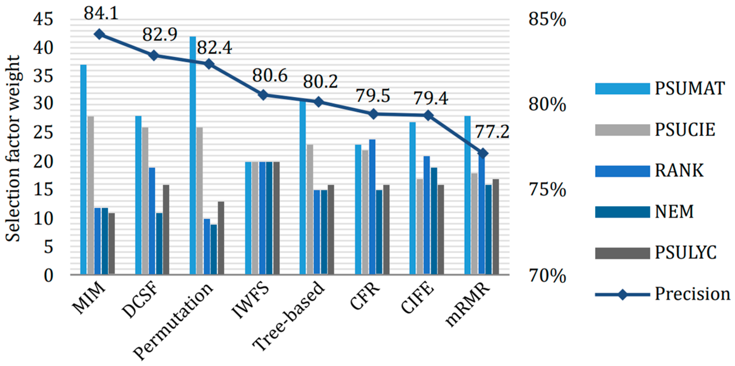
For this procedure, the same filters from the previous process are executed, most of which produce X s = PSUMAT when requiring only one feature, except for DCSF, CFR, and IWFS, which report X s = TAMFAM. With the relevant variable factor obtained with MIM, 1.33; the score for the preselected attribute is obtained. With the filter scores transformed into weights (Figure 10), PJEPOST_1 is obtained. Then, with this fictitious score, the machine is trained to predict AP based on an RF algorithm with 10 trees (NN is biased when predicting) based on impurity discrimination by entropy, adjusted with a six-fold stratified CV and hyperparameter grid, and is validated and evaluated by measuring its precision (Figure 10).
To ensure the reliability of the result, given s 0.02 , the F score and AUC-ROC are measured for MIM and DCSF, obtaining: F M I M = 80.3 % , A U C M I M = 0.79 , F D C S F = 69.7 % , A U C M I M = 0.73 . Additionally, the correlation between PJEPOST_1 and AP is measured, obtaining r S p e a r m a n = 0.42 (value p = 3.1 × 10−160) for MIM and r S p e a r m a n = 0.37 (value p = 3.9 × 10−121) for DCSF. Therefore, the weights obtained with MIM generate the best association with AP. Wrappers, on the other hand, do not allow for weight rankings; neither do embedded methods, as they cannot avoid negative scores in some SC.

4. Discussions

4.1. Improvement in Precision Through Concept Drift and Outlier Management

To evaluate the incorporation of CD and outlier management processes, the precision obtained in predicting AP using the original cleaned matrix is compared with the precision obtained after executing these processes. Using a multilayer neural network with cross-validation and grid search, 14 neurons in the input layer and 1 in the output layer, and various combinations of one and two hidden layers for a total of 8 neurons, the procedure is iterated 10 times to generate results with a 98% confidence level. The average precision with the original matrix is 78.1%, in the range [77.2%; 79.0%]. After the CD management process, the average precision increases to 78.9%, with a confidence interval between 78.0% and 79.7%. This result demonstrates a slight but positive effect, justifying the inclusion of this process.
Similarly, operating the network with a matrix post-outlier management (without CD management) results in an average precision of 78.9%, with a confidence interval between 78.3% and 79.5%. Thus, a slight positive effect is also observed when including outlier management. When both processes are applied, the average precision increases to 79.0%, with a confidence interval between 78.0% and 79.9%.

4.2. Validity of the Optimal Subset of Features

A precision of 82.5% in predicting academic performance was achieved using an optimal subset of features. This precision is significantly higher than that obtained with the cleaned original matrix, which reached 78.1% (with a confidence interval between 77.2% and 79.0%). This demonstrates that the proposed methodology improves the predictive capability of the model by 4.4 percentage points.
Within the optimal subset, the five SCs are the most important features, contributing 95% of the necessary information to predict academic performance. This is because their individual contribution is over 10%, while that of each of the other attributes is less than 1.6%.
Among the other relevant features are ESTUPAD and DECIL, each contributing 28%, followed by PRIGE with 16%. This suggests that the educational level of the parents, the socioeconomic level, and proximity to the educational institution are also important factors to consider in predicting academic performance.

4.3. Predictive Ability with Obtained Weights

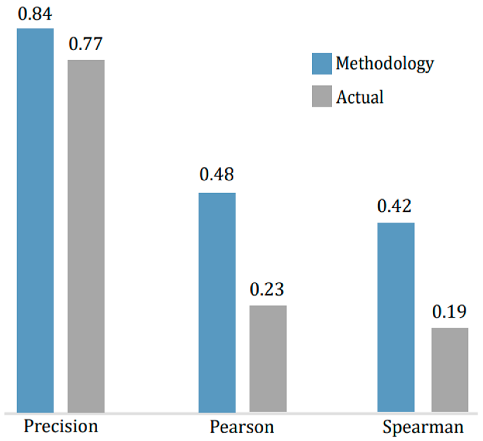
The ability to predict AP is compared between the obtained score PJEPOST_1 and the real score PJEPOST. Using an RF model and an entropy-based discrimination criterion with 10 estimators, a precision of 84.1% is achieved, compared to the 77.0% obtained with the real score. This demonstrates a greater association between the AP and the SC weighted according to the MIM algorithm, along with a greater predictive ability of the model.
Additionally, the correlation values with the AP obtained through MIM and the real values are compared using Pearson and Spearman coefficients. With MIM, a Pearson coefficient of 0.48 (value p = 1.4 × 10−221) and a Spearman coefficient of 0.42 (value p = 3.1 × 10−160) are obtained, significantly higher than the real values of 0.23 y 0.19, respectively, with a p-value <= 2.7 × 10⁻³¹ (Figure 11). Therefore, the weighting of SC obtained with the proposed methodology is more robustly associated with AP than the real weighting.

4.4. Methodological Justification and Data Validity in the Optimization of the Admission Process

This study focuses on developing and validating a methodology to enhance the prediction of academic performance based on admission criteria, rather than providing an immediate operational solution. To achieve this, it incorporates strategies to mitigate the impact of data distribution changes, including concept drift detection and management, as well as stratified cross-validation, thereby improving its generalizability across diverse contexts.
While the analyzed data spans the period from 2014 to 2018, the methodology remains adaptable with more recent data without affecting the validity of the general conclusions. A significant contribution of this study is demonstrating the potential insufficiency of traditional models, which rely on stationarity assumptions, thereby highlighting the need for dynamic modeling and optimized variable selection. Consequently, the proposed methodology is not only applicable to the dataset utilized but can also be adapted for the continuous optimization of the admission process.

5. Conclusions

This research contributes to the field of educational administration by developing and validating a machine learning-based methodology. Using classification algorithms, CD detection, outlier management, and feature selection, this approach optimizes the weighting of selection criteria in university admissions and identifies a subset of features that significantly enhance the precision of predicting first-year academic performance.
While this study’s methodology does not establish a direct link with educational management, it enhances the university admissions process by integrating rigorous scientific assessments. This suggests that process optimization, aided by ML, could significantly impact educational management.
The administrators can justify the adoption of the new selection process by highlighting the use of advanced technologies, such as ML, that optimize academic evaluation. These tools enable more objective assessments, mitigating the biases inherent in traditional methods. To build trust, it is crucial to transparently communicate that the system prioritizes impartial evaluation of academic merit. Furthermore, it is essential to guarantee inclusion through feedback mechanisms with the community/society that foster continuous improvement.
In the context of admission to engineering programs at a public Chilean university, its application is validated with a weighting of SC that resulted in an application score that predicts first-year approval with a precision of 84.1% ( p T = 82.3 % ) versus 77.0% ( p T = 77.1 % ) of the real score. This improvement is reflected in a stronger product-moment correlation with dichotomous AP, r P = 0.48 (value p = 1.4 × 10−221), compared to r P = 0.23 (value p = 3.7 × 10−49) of the real score.
The prediction model, obtained with a multilayer perceptron neural network, has a precision of 82.5% ( p T = 79.0 % ), which implies a high association with academic performance, compared to 78.1% ( p T = 77.3 % ) of the initial dataset, and a high generalization ability, compared to its performance in training. The subset of features includes the five selection criteria, plus the father’s education, socioeconomic level, graduation seniority, application preference, first-generation university status, major, department, and gender, and excludes family size.
It is demonstrated that it is incorrect to assume the stationarity of the data when analyzing a university admission process. In this research, a significant change in concept was detected, mainly due to a variation in the distribution of one of the features. Managing this change allowed for an increase in the model’s accuracy by one percentage point.
The methodology demonstrates the importance of establishing appropriate performance measurement instruments to evaluate the model. These instruments not only determine the validity and reliability of the results but also help to avoid overfitting, which can be mitigated by using a cost matrix or function, depending on whether it is a categorical or continuous target. In the present context, the use of the precision measure is suggested.
The use of filters and embedded algorithms revealed that the MIM filter provides the best subset and weighting ranking, indicating that the selection criteria are defined independently of the redundancy and complementarity between them.
Compared to traditional methods, the algorithms used considered the interaction between variables and the model’s evaluation on a holdout sample, thus ensuring true prediction. The application of cross-validation, along with confirming that the model’s performance did not exceed during training, ensured the absence of overfitting. Neural networks demonstrated the best classification performance, as in other studies focused on engineering students (Contreras et al., 2020; Rachburee & Punlumjeak, 2015), although in different contexts.
This study innovates in the design of processes and algorithmic procedures that aim to increase the efficiency of university admissions, which incorporate the management of CD and outliers, establish precision as a performance measurement instrument, and generate a ranking for selection criteria. Although the obtained values are not guaranteed in other contexts, the methodology contributes to the improvement of the student selection process and the theoretical development of academic performance prediction.
In summary, the proposed methodology ensures a reliable, valid, and unbiased selection process by carefully addressing the main sources of error in traditional methods.
First, it avoids model bias by employing machine learning models that rigorously separate training and testing performance. This approach accommodates data complexity beyond the limitations of statistical regression (e.g., restricted to linear relationships and normally distributed data, among others).
Additionally, it addresses sampling bias both in the arbitrary selection of cohorts and the inclusion of outliers through concept drift management and outlier detection. This approach allows for the analysis of temporal dynamics and the elimination of noise in the data.
On the other hand, it overcomes evaluation bias by considering the cost matrix in selecting the performance measurement tool. These elements not only ensure reliability by predicting data different from the training set and calculating confidence intervals but also strengthen the validity of the analysis, guaranteed by the scientific and rigorous measurement of the performance of optimized algorithmic models.
The robustness of the results obtained with this methodology empowers higher education administrators to make objective and justifiable decisions. This approach ensures a fair, transparent, and context-specific process tailored to the specific study.
For future studies, it is suggested to consider additional variables that may affect academic performance. Regarding the management of outliers, alternative techniques such as semi-supervised learning or supervised learning based on vocational information and/or student dropout data can be explored. The evaluation of the models could be enriched by generating a cost matrix or function, adjusted to the specific definition of academic performance. Additionally, the use of other feature selection technologies is recommended for the search for the optimal subset and ranking of factors.

Author Contributions

Conceptualization, M.H., M.V. and M.A.; methodology, M.H. and R.T.; software, M.H. and P.S.; validation, G.F., R.T. and M.V.; formal analysis, M.A. and P.S.; investigation, M.H. and R.T.; resources, M.A.; data curation, M.V.; writing—original draft preparation, G.F. and M.V.; writing—review and editing, P.S.; visualization, G.F.; supervision, R.T.; project administration, G.F.; funding acquisition, M.A. and P.S. All authors have read and agreed to the published version of the manuscript.

Funding

This research has been supported by the DICYT (Scientific and Technological Research Bureau) of the University of Santiago of Chile (USACH) and the Department of Industrial Engineering. Likewise, we appreciate the support of the Faculty of Engineering of the Universidad de Santiago de Chile.

Institutional Review Board Statement

Not applicable.

Informed Consent Statement

Not applicable.

Data Availability Statement

The data presented in this study are available on request from the corresponding author.

Conflicts of Interest

The authors declare no conflicts of interest.

Notations

FSFeature selection
CVCross-validation
CDConcept drift
SCSelection criteria
APAcademic performance
r P Pearson coefficient
MLMachine learning
NNNeural networks
DEDemographic
ACAcademic
SESocioeconomic
kNNk-nearest neighbors
MIMMutual information maximization
JMIJoint mutual information
CFRComposition of feature relevancy
MRIMaximal relevance and maximal independence
EDAExploratory data analysis
CMIMConditional mutual information maximization criterion
HBGBHistogram-based gradient boosting tree
DCSFDynamic change in the selected feature
MIFSMutual information-based feature selection
CIFEConditional infomax feature extraction
IWFSInteraction weight-based feature selection
mRMRMinimal redundancy maximal relevance

References

  1. Abdel-Basset, M., Ding, W., & El-Shahat, D. (2021). A hybrid Harris Hawks optimization algorithm with simulated annealing for feature selection. Artificial Intelligence Review, 54(1), 593–637. [Google Scholar] [CrossRef]
  2. Adeyemo, A. B., & Kuyoro, S. O. (2013). Investigating the effect of students socio-economic/family background on students academic performance in tertiary institutions using decision tree algorithm. Journal of Life & Physical Sciences, 4(2), 61–78. Available online: https://www.researchgate.net/publication/370205648_Investigating_the_Effect_of_Students_Socio-EconomicFamily_Background_on_Students_Academic_Performance_in_Tertiary_Institutions_using_Decision_Tree_Algorithm (accessed on 10 October 2024).
  3. Affendey, L., Paris, I., Mustapha, N., Sulaiman, M., & Muda, Z. (2010). Ranking of influencing factors in predicting students’ academic performance. Information Technology Journal, 9(4), 832–837. [Google Scholar] [CrossRef]
  4. Aguayo-Hernández, C. H., Sánchez Guerrero, A., & Vázquez-Villegas, P. (2024). The learning assessment process in higher education: A grounded theory approach. Education Sciences, 14(9), 984. [Google Scholar] [CrossRef]
  5. Alalawi, K., Athauda, R., & Chiong, R. (2024). An extended learning analytics framework integrating machine learning and pedagogical approaches for student performance prediction and intervention. International Journal of Artificial Intelligence in Education, 1–49. [Google Scholar] [CrossRef]
  6. Albreiki, B., Zaki, N., & Alashwal, H. (2021). A systematic literature review of student’ performance prediction using machine learning techniques. Education Sciences, 11(9), 552. [Google Scholar] [CrossRef]
  7. Al-Okaily, M., Magatef, S., Al-Okaily, A., & Shehab Shiyyab, F. (2024). Exploring the factors that influence academic performance in Jordanian higher education institutions. Heliyon, 10(13), e33783. [Google Scholar] [CrossRef]
  8. Amini, F., & Hu, G. (2021). A two-layer feature selection method using genetic algorithm and elastic net. Expert Systems with Applications, 166, 114072. [Google Scholar] [CrossRef]
  9. Anaconda. (2024). The operating system for AI. Available online: https://www.anaconda.com/ (accessed on 10 October 2024).
  10. Battiti, R. (1994). Using mutual information for selecting features in supervised neural net learning. IEEE Transactions on Neural Networks, 5(4), 537–550. [Google Scholar] [CrossRef]
  11. Chorev, S., Tannor, P., Israel, D. B., Bressler, N., Gabbay, I., Hutnik, N., Liberman, J., Perlmutter, M., Romanyshyn, Y., & Rokach, L. (2022). Deepchecks: A library for testing and validating machine learning models and data. Journal of Machine Learning Research, 23(285), 1–6. Available online: http://jmlr.org/papers/v23/22-0281.html (accessed on 10 October 2024).
  12. Contreras, L. E., Fuentes, H. J., & Rodríguez, J. I. (2020). Academic performance prediction by machine learning as a success/failure indicator for engineering students. Formación Universitaria, 13(5), 233–246. [Google Scholar] [CrossRef]
  13. Cunningham, P., & Delany, S. J. (2021). K-nearest neighbour classifiers—A tutorial. ACM Computing Surveys, 54(6). [Google Scholar] [CrossRef]
  14. d’Astous, P., & Shore, S. H. (2024). Human capital risk and portfolio choices: Evidence from university admission discontinuities. Journal of Financial Economics, 154, 103793. [Google Scholar] [CrossRef]
  15. Deepchecks. (2023). Deepchecks documentation. Available online: https://docs.deepchecks.com/en/stable/getting-started/welcome.html (accessed on 10 October 2024).
  16. Deepika, K., & Sathyanarayana, N. (2022). Relief-F and budget tree random forest based feature selection for student academic performance prediction. International Journal of Intelligent Engineering and Systems, 12(1), 30–39. [Google Scholar] [CrossRef]
  17. DEMRE. (2022). Instrumentos de acceso, especificaciones y procedimientos. Available online: https://demre.cl/publicaciones/2023/2023-22-06-07-instrumentos-acceso-p2023 (accessed on 10 October 2024).
  18. Echegaray-Calderon, O. A., & Barrios-Aranibar, D. (2016, October 13–16). Optimal selection of factors using Genetic Algorithms and Neural Networks for the prediction of students’ academic performance. Latin-America Congress on Computational Intelligence (pp. 1–6), Curitiba, Brazil. [Google Scholar] [CrossRef]
  19. Eshet, Y. (2024). Academic integrity crisis: Exploring undergraduates’ learning motivation and personality traits over five years. Education Sciences, 14(9), 986. [Google Scholar] [CrossRef]
  20. Espinoza, O., González, L., Sandoval, L., Corradi, B., McGinn, N., & Vera, T. (2024a). The impact of non-cognitive factors on admission to selective universities: The case of Chile. Educational Review, 76(4), 979–995. [Google Scholar] [CrossRef]
  21. Espinoza, O., Sandoval, L., González, L. E., Corradi, B., McGinn, N., & Vera, T. (2024b). Did free tuition change the choices of students applying for university admission? Higher Education, 87(5), 1317–1337. [Google Scholar] [CrossRef]
  22. Fleuret, F. (2004). Fast binary feature selection with conditional mutual information. Journal of Machine Learning Research, 5, 1531–1555. [Google Scholar]
  23. Frías-Blanco, I., Del Campo-Ávila, J., Ramos-Jiménez, G., Morales-Bueno, R., Ortiz-Díaz, A., & Caballero-Mota, Y. (2015). Online and non-parametric drift detection methods based on Hoeffding’s bounds. IEEE Transactions on Knowledge and Data Engineering, 27(3), 810–823. [Google Scholar] [CrossRef]
  24. Fuertes, G., Vargas Guzman, M., Soto Gomez, I., Witker Riveros, K., Peralta Muller, M. A., & Sabattin Ortega, J. (2015). Project-based learning versus cooperative learning courses in engineering students. IEEE Latin America Transactions, 13(9), 3113–3119. [Google Scholar] [CrossRef]
  25. Gama, J., Medas, P., Castillo, G., & Rodrigues, P. (2004). Learning with drift detection. Symposium on Artificial Intelligence, 3171, 286–295. [Google Scholar] [CrossRef]
  26. Gao, W., Hu, L., & Zhang, P. (2018a). Class-specific mutual information variation for feature selection. Pattern Recognition, 79, 328–339. [Google Scholar] [CrossRef]
  27. Gao, W., Hu, L., Zhang, P., & He, J. (2018b). Feature selection considering the composition of feature relevancy. Pattern Recognition Letters, 112, 70–74. [Google Scholar] [CrossRef]
  28. Github. (2024). University feature selection library ITMO. Available online: https://github.com/ctlab/ITMO_FS (accessed on 10 October 2024).
  29. Granger, B. E., & Perez, F. (2021). Jupyter: Thinking and storytelling with code and data. Computing in Science and Engineering, 23(2), 7–14. [Google Scholar] [CrossRef]
  30. Guo, H., Zhang, S., & Wang, W. (2021). Selective ensemble-based online adaptive deep neural networks for streaming data with concept drift. Neural Networks, 142, 437–456. [Google Scholar] [CrossRef] [PubMed]
  31. Harsono, S., Utami, E., & Yaqin, A. (2024, February 21). The association rule methods and k-means clustering for optimization mapping of new students admission. International Conference on Artificial Intelligence and Mechatronics System, Bandung, Indonesia. [Google Scholar] [CrossRef]
  32. Hashmani, M. A., Jameel, S. M., Rehman, M., & Inoue, A. (2020). Concept drift evolution in machine learning approaches: A systematic literature review. International Journal on Smart Sensing and Intelligent Systems, 13(1), 1–16. [Google Scholar] [CrossRef]
  33. Hilbert, S., Coors, S., Kraus, E., Bischl, B., Lindl, A., Frei, M., Wild, J., Krauss, S., Goretzko, D., & Stachl, C. (2021). Machine learning for the educational sciences. Review of Education, 9(3), e3310. [Google Scholar] [CrossRef]
  34. Hinojosa, M. F. (2021). Adaptation of the balanced scorecard to Latin American higher education institutions in the context of strategic management: A systematic review with meta-analysis. In International conference of production research-Americas, 1408 CCIS (pp. 125–140). Springer. [Google Scholar] [CrossRef]
  35. Huang, S. H. (2015). Supervised feature selection: A tutorial. Artificial Intelligence Research, 4(2), 22–37. [Google Scholar] [CrossRef]
  36. Jeong, Y. S., Shin, K. S., & Jeong, M. K. (2015). An evolutionary algorithm with the partial sequential forward floating search mutation for large-scale feature selection problems. Journal of the Operational Research Society, 66(4), 529–538. [Google Scholar] [CrossRef]
  37. Li, Y., Li, T., & Liu, H. (2017). Recent advances in feature selection and its applications. Knowledge and Information Systems, 53(3), 551–577. [Google Scholar] [CrossRef]
  38. Lin, D., & Tang, X. (2006, May 7–13). Conditional infomax learning: An integrated framework for feature extraction and fusion. European Conference on Computer Vision, 3951 LNCS (pp. 68–82), Graz, Austria. [Google Scholar] [CrossRef]
  39. Lu, J., Liu, A., Dong, F., Gu, F., Gama, J., & Zhang, G. (2019). Learning under concept drift: A review. IEEE Transactions on Knowledge and Data Engineering, 31(12), 2346–2363. [Google Scholar] [CrossRef]
  40. Marbouti, F., Ulas, J., & Wang, C. H. (2021). Academic and demographic cluster analysis of engineering student success. IEEE Transactions on Education, 64(3), 261–266. [Google Scholar] [CrossRef]
  41. Matsushita, R. (2024). Toward an ecological view of learning: Cultivating learners in a data-driven society. Educational Philosophy and Theory, 56(2), 116–125. [Google Scholar] [CrossRef]
  42. Mineduc. (2008). Estudio sobre causas de la deserción universitaria. Available online: https://bibliotecadigital.mineduc.cl/handle/20.500.12365/17988 (accessed on 10 October 2024).
  43. Palacios, C. A., Reyes-Suárez, J. A., Bearzotti, L. A., Leiva, V., & Marchant, C. (2021). Knowledge discovery for higher education student retention based on data mining: Machine learning algorithms and case study in Chile. Entropy, 23(4), 485. [Google Scholar] [CrossRef]
  44. Pan, J., Zou, Z., Sun, S., Su, Y., & Zhu, H. (2022). Research on output distribution modeling of photovoltaic modules based on kernel density estimation method and its application in anomaly identification. Solar Energy, 235, 1–11. [Google Scholar] [CrossRef]
  45. Peng, H., Long, F., & Ding, C. (2005). Feature selection based on mutual information: Criteria of max-dependency, max-relevance, and min-redundancy. IEEE Transactions on Pattern Analysis and Machine Intelligence, 27(8), 1226–1238. [Google Scholar] [CrossRef]
  46. Pilnenskiy, N., & Smetannikov, I. (2020). Feature selection algorithms as one of the python data analytical tools. Future Internet, 12(3), 54. [Google Scholar] [CrossRef]
  47. Putpuek, N., Rojanaprasert, N., Atchariyachanvanich, K., & Thamrongthanyawong, T. (2018, June 6–8). Comparative study of prediction models for final gpa score: A case study of rajabhat rajanagarindra university. International Conference on Computer and Information Science (pp. 92–97), Singapore. [Google Scholar] [CrossRef]
  48. Rachburee, N., & Punlumjeak, W. (2015, October 29–30). A comparison of feature selection approach between greedy, IG-ratio, Chi-square, and mRMR in educational mining. International Conference on Information Technology and Electrical Engineering: Envisioning the Trend of Computer, Information and Engineering (pp. 420–424), Chiang Mai, Thailand. [Google Scholar] [CrossRef]
  49. Rawal, A., & Lal, B. (2023). Predictive model for admission uncertainty in high education using Naïve Bayes classifier. Journal of Indian Business Research, 15(2), 262–277. [Google Scholar] [CrossRef]
  50. Shmueli, G., & Koppius, O. R. (2011). Predictive analytics in information systems research. MIS Quarterly, 35(3), 553–572. [Google Scholar] [CrossRef]
  51. United Nations. (n.d.). Transforming our world: The 2030 agenda for sustainable development. Available online: https://sdgs.un.org/2030agenda (accessed on 8 October 2024).
  52. Uvidia Fassler, M. I., Cisneros Barahona, A. S., Dumancela Nina, G. J., Samaniego Erazo, G. N., & Villacrés Cevallos, E. P. (2020). Application of knowledge discovery in data bases analysis to predict the academic performance of university students based on their admissions test. In M. Botto-Tobar, J. León-Acurio, A. Díaz Cadena, & P. Montiel Díaz (Eds.), The international conference on advances in emerging trends and technologies, ICAETT 2019 (Vol. 1066, pp. 485–497). Springer. [Google Scholar] [CrossRef]
  53. Van Rossum, G., & Drake, F. L. (2003). An introduction to python. Network Theory Ltd. [Google Scholar]
  54. Vargas, M., Alfaro, M., Fuertes, G., Gatica, G., Gutiérrez, S., Vargas, S., Banguera, L., & Durán, C. (2019). CDIO project approach to design polynesian canoes by first-year engineering students. International Journal of Engineering Education, 35(5), 1336–1342. [Google Scholar]
  55. Vargas, M., Nuñez, T., Alfaro, M., Fuertes, G., Gutierrez, S., Ternero, R., Sabattin, J., Banguera, L., Durán, C., & Peralta, M. A. (2020). A project based learning approach for teaching artificial intelligence to undergraduate students. International Journal of Engineering Education, 36(6), 1773–1782. [Google Scholar]
  56. Velmurugan, T., & Anuradha, C. (2016). Performance evaluation of feature selection algorithms in educational data mining. Performance Evaluation, 5(2), 131–139. [Google Scholar]
  57. Venkatesh, B., & Anuradha, J. (2019). A review of feature selection and its methods. Cybernetics and Information Technologies, 19(1), 3–26. [Google Scholar] [CrossRef]
  58. Vergara-Díaz, G., & Peredo-López, H. (2017). Relación del desempeño académico de estudiantes de primer año de universidad en Chile y los instrumentos de selección para su ingreso. Revista Educación, 41(2), 95–104. [Google Scholar] [CrossRef]
  59. Wainer, J., & Cawley, G. (2021). Nested cross-validation when selecting classifiers is overzealous for most practical applications. Expert Systems with Applications, 182, 115222. [Google Scholar] [CrossRef]
  60. Wan, J., Chen, H., Li, T., Huang, W., Li, M., & Luo, C. (2022). R2CI: Information theoretic-guided feature selection with multiple correlations. Pattern Recognition, 127, 108603. [Google Scholar] [CrossRef]
  61. Wang, J., Wei, J. M., Yang, Z., & Wang, S. Q. (2017). Feature selection by maximizing independent classification information. IEEE Transactions on Knowledge and Data Engineering, 29(4), 828–841. [Google Scholar] [CrossRef]
  62. Wang, L., Jiang, S., & Jiang, S. (2021). A feature selection method via analysis of relevance, redundancy, and interaction. Expert Systems with Applications, 183, 115365. [Google Scholar] [CrossRef]
  63. Webb, G. I., Hyde, R., Cao, H., Nguyen, H. L., & Petitjean, F. (2016). Characterizing concept drift. Data Mining and Knowledge Discovery, 30(4), 964–994. [Google Scholar] [CrossRef]
  64. Williams, D. (2021). Imaginative constraints and generative models. Australasian Journal of Philosophy, 99(1), 68–82. [Google Scholar] [CrossRef]
  65. Wu, X., & Wu, J. (2020). Criteria evaluation and selection in non-native language MBA students admission based on machine learning methods. Journal of Ambient Intelligence and Humanized Computing, 11(9), 3521–3533. [Google Scholar] [CrossRef]
  66. Xu, S., & Wang, J. (2017). Dynamic extreme learning machine for data stream classification. Neurocomputing, 238, 433–449. [Google Scholar] [CrossRef]
  67. Yang, H. H., & Moody, J. (1999). Data visualization and feature selection: New algorithms for nongaussian data. Advances in Neural Information Processing Systems, 12, 687–693. [Google Scholar]
  68. Yang, Z., Al-Dahidi, S., Baraldi, P., Zio, E., & Montelatici, L. (2020). A novel concept drift detection method for incremental learning in nonstationary environments. IEEE Transactions on Neural Networks and Learning Systems, 31(1), 309–320. [Google Scholar] [CrossRef]
  69. Yarkoni, T., & Westfall, J. (2017). Choosing prediction over explanation in psychology: Lessons from machine learning. Perspectives on Psychological Science, 12(6), 1100–1122. [Google Scholar] [CrossRef]
  70. Zeng, Z., Zhang, H., Zhang, R., & Yin, C. (2015). A novel feature selection method considering feature interaction. Pattern Recognition, 48(8), 2656–2666. [Google Scholar] [CrossRef]
  71. Zhao, Y., Nasrullah, Z., & Li, Z. (2019). PyOD: A python toolbox for scalable outlier detection. Journal of Machine Learning Research, 20(96), 1–7. Available online: http://jmlr.org/papers/v20/19-011.html (accessed on 10 October 2024).
  72. Zhou, X., Lo Faro, W., Zhang, X., & Arvapally, R. S. (2019). A framework to monitor machine learning systems using concept drift detection. International Conference Business Information Systems, 353, 218–231. [Google Scholar] [CrossRef]
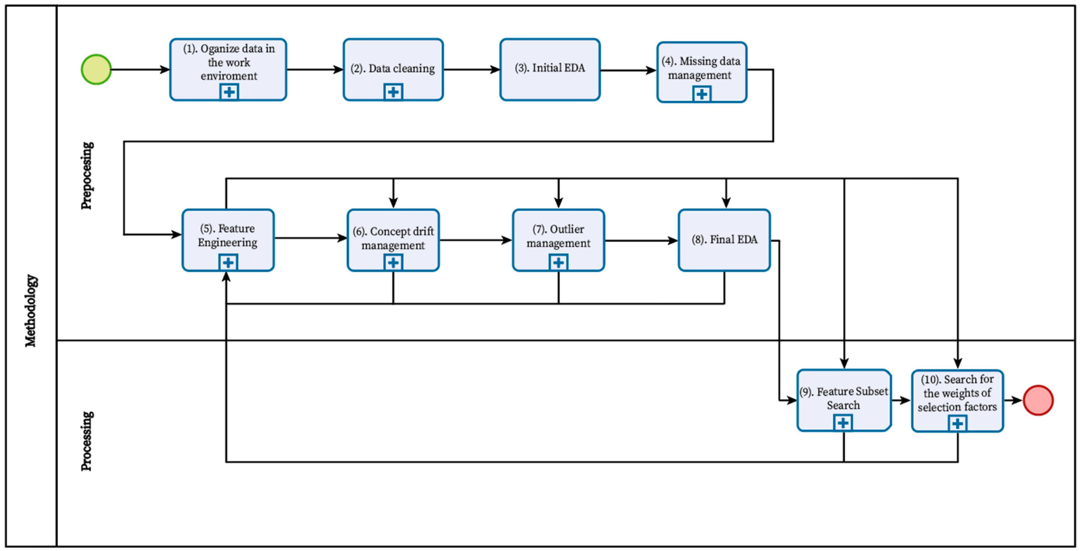
Figure 1. Flowchart of the proposed methodology.
Education 15 00326 g001
Figure 2. CD management flowchart.
Education 15 00326 g002
Figure 3. Outlier management flowchart.
Education 15 00326 g003
Figure 4. Subset search flowchart.
Education 15 00326 g004
Figure 5. Flowchart for finding selection criteria weights.
Education 15 00326 g005
Figure 6. Evolution of model performance between cohorts with random forests and neural networks.
Education 15 00326 g006
Figure 7. Mean absolute error (MAE) of each detection algorithm for the 2015 cohort.
Education 15 00326 g007
Figure 8. Subsets whose explanatory capacity exceeds the threshold.
Education 15 00326 g008
Figure 9. Association between features and AP according to the MIM filter.
Education 15 00326 g009
Figure 10. Predictive performance of the RF model considering the weights obtained with the different algorithms.
Education 15 00326 g010
Figure 11. Difference in precision and correlation between the application score with the obtained and actual weights.
Education 15 00326 g011
Table 1. Feature selection methodologies in machine learning applied to the academic context.
Ref.DomainAcademic ProgramVariablesTasks and AlgorithmsPerformance
(Wu & Wu, 2020)Determine the influence of factors on admission and final AP.AdministrationInput: 20 academic, demographic, and personal variables.
Output: Continuous grade point average.
REG: RLR, SVM, RF, GBDT, LR
FS: Relevance with R and ReliefF, and redundancy with R.
Without FS: MAE-SVM = 3.38, RMSE-SVM = 4.48.
With FS: MAE-SVM = 3.41, RMSE-SVM = 4.48
(Contreras et al., 2020)Determine the variables that most influence APEngineeringInput: Admission tests, socioeconomic, demographic, cultural, institutional, and personal data.
Output: Categorized AP.
CL: DT, kNN, NN, SVM.
FS: Chi2; ANOVA; Pearson; RFE with LgR, LR, and SVM; RF and BS with DT.
pSVM with FS = 0.61. SVM and NN are the best
(Putpuek et al., 2018)Compare two prediction models for APEducationInput: Demographic, socioeconomic, academic.
Output: Final grade point average.
CL: DT, NB, kNN
FS: SFS, BS, EFS
pID3 = 28.9%
NB higher Acc = 43%
(Adeyemo & Kuyoro, 2013)Evaluate the effect of socioeconomic background on APAllInput: Socioeconomic, demographic, and academic.
Output: Cumulative grade point average of the 1st year in 7 classes.
CL: DT
FS: CFS and COE, importance with CFS and COE wrappers.
pC4.5 (DT) = 73.3%
(Echegaray-Calderon & Barrios-Aranibar, 2016)Identify the factors that affect APAllInput: Demographic, socioeconomic, academic admission, and current data.
Output: AP of 5 classes.
CL: NN
FS: GA, the importance of GA
Without FS: Acc = 89%
With FS: Acc = 80%
(Rachburee & Punlumjeak, 2015)Compare FS methods to improve the prediction of APEngineeringInput: Demographic and academic admission data; 15 in total.
Output: Grade point average in 3 classes.
CL: NB, DT, kNN, NN
FS: Chi2, IG, mRMR, SFS
AccSFS (NN) = 91%
(Velmurugan & Anuradha, 2016)Compare the performance of various FS techniques in predicting exam scoresHigh schoolInput: Demographic, socioeconomic, academic (admission), and current data.
Output: Final exam score in 4 classes.
CL: DT, NB, kNN
FS: CFS, BFS, Chi2, IG, Relief
Usan Weka
With FS: pCFS(NB) = 99.8%.
Best classifier IBK (kNN)p = 99.7%
(Affendey et al., 2010)Rank the factors contributing to the prediction of APInformaticsInput: AP in subjects.
Output: Dichotomous AP.
NB, DT, NN.AccNB = 93%
(Deepika & Sathyanarayana, 2022)Select active features to reduce high dimensionality and manage data uncertainty using the hybrid method RFBT-RFAllNo informationDT, NB, SVM, and KNN. Acc RFBT-RF between 81.5% and 97.9%,
CL: classification, REG: regression.
Table 2. Variables considered in the research: DE, SE, and AC.
Variable NameDescription
DE_COHORTEYear the student enrolled at the university.
DE_ANTEGRENumber of years from the student’s high school graduation year to the year of application.
DE_NACNationality of the student.
DE_REGIONDetermines whether the student is from the Metropolitan Region or another region, according to their place of origin.
DE_GENEGender of the student.
DE_TAMFAMNumber of family members of the student.
AC_DEPAName of the department to which the student’s major belongs.
AC_CARRName of the student’s major.
SE_DECILSocioeconomic level of the student as per capita household income.
SE_ESTUMADMother’s level of education.
SE_ESTUPADFather’s level of education.
SE_PRIGEDetermines if the student is the first in their family to attend university.
SE_ESTADEPAdministrative dependency of the high school from which the student graduated.
SE_ESTADIFDifferentiated high school education at the student’s graduating institution.
AC_PREFPOSTThe preferred major choice at the time of the student’s application.
AC_PSUMATScore on the mathematics admission test PSUMAT.
AC_PSULYCScore on the language and communication admission test PSULYC.
AC_PSUPROMAverage score of PSUMAT and PSULYC.
AC_PSUCIEScore on the science admission test PSUCIE.
AC_NEMScore equivalent to the average grade in high school NEM.
AC_RANKScore equivalent to the high school ranking.
AC_ PJEPOSTWeighted or application score for engineering programs.
APThe number of courses passed is divided by the number of courses enrolled in the first year.
Table 3. Discretization of the target variable AP.
Numerical ScaleConceptual ScalePercentage ScaleNumber of Cases
7.0A = excellent1001117
[6.0; 7]B = very good[86; 100]715
[5.0; 6.0]C = good[73; 86]1310
[4.0; 5.0]D = sufficient[60; 73]1001
[2.5; 4.0]E = insufficient[30; 60]1488
[1.0; 2.5]F = bad[0; 30]569
Table 4. Detection and characterization of concept drift.
Indicator2014–20152015–20162016–20172017–2018
Meets DV < 0.26YesNoYesNo
DV0.170.260.250.73
Variables that contribute the most to the driftPJEPOST (58%)
CARR (24%)
PREFPOST (82%)
CARR (15%)
DECIL (91%)ESTUPAD (100%)
Table 5. Minimum and maximum percentages of students per cohort drop out due to vocational reasons or lack of skills, according to the literature.
Item\Cohort (Number of Cases)2014 (1244 Cases)2015 (1196 Cases)2016 (875 Case)2017 (792 Cases)
Dropout rate (%)12192521
Minimum Dropout by Vocation30% × 12% = 3.6%30% × 19% = 5.7%30% × 25% = 7.5%30% × 21% = 6.3%
Maximum Dropout by Vocation66% × 12% = 7.92%66% × 19% = 12.54%66% × 25% = 16.5%66% × 21% = 13.86%
Minimum Dropout by Skills14% × 12% = 1.68%14% × 19% = 2.7%14% × 25% = 3.5%14% × 21% = 2.94%
Maximum Dropout by Skills33% × 12% = 3.96%33% × 19% = 6.3%33% × 25% = 8.25%33% × 21% = 6.93%
Minimum Total Dropout5.28% (3.6% + 1.68%)8.4% (5.7% + 1.68%)11% (7.5% + 3.5%)9.2% (6.3% + 2.94%)
Maximum Total Dropout11.88% (7.92% + 3.96%)18.84% (12.54% + 6.3%)24.75% (16.50% + 8.25%)20.79% (13.86% + 6.93%)
Disclaimer/Publisher’s Note: The statements, opinions and data contained in all publications are solely those of the individual author(s) and contributor(s) and not of MDPI and/or the editor(s). MDPI and/or the editor(s) disclaim responsibility for any injury to people or property resulting from any ideas, methods, instructions or products referred to in the content.