Concentrated Post-2020 Sigma Widening: Metric Sensitivity and Persistent Income Hierarchies in Cross-Country GDP per Capita Data

Abstract

Post-2020 changes in cross-country log GDP per capita dispersion are directionally consistent across macroeconomic data systems but concentrated in a few country trajectories. Using the IMF WEO 1980–2024 baseline, a provisional 2025 extension, and a 167-country WEO–WDI–PWT panel for 2000–2023, the analysis compares sigma, level inequality, weighting, contributions, mobility, and horizon. Sigma rises by 0.018–0.024 across the sources. Paired country-resampling intervals support sign stability, not broad-based widening. The top five contributors account for 60.3–66.9% of the variance increase and the top ten for 86.6–96.3%; positive residuals remain after joint exclusion. The WEO 2020–2024 increase was exceeded by only two of the 36 preceding four-year changes, although sigma in 2024 remained below its 2000 level. Gini and Theil decline or remain approximately flat, while fixed-quartile separation and persistent ranks locate the change within a durable hierarchy. The contribution is an integrated diagnostic of scale, weighting, concentration, persistence, and horizon; it neither measures global interpersonal inequality nor establishes a structural reversal of long-run convergence.

1. Introduction

After 2020, the cross-sectional standard deviation of log GDP per capita increases across WEO, WDI, and PWT, whereas unweighted and population-weighted Gini and Theil measures do not show a corresponding general increase. The research problem is therefore not whether every inequality indicator moved upward, but how a source-consistent positive sigma change can coexist with flatter level-based measures and persistent country ranks. The manuscript distinguishes the direction of the aggregate statistic from the breadth of country-level widening.

The empirical objects are complementary rather than interchangeable. Beta convergence summarizes average growth-rate catching-up; sigma records dispersion in log income; Gini and Theil summarize level-income inequality under alternative weighting; contributor diagnostics identify concentration; and rank or transition measures record positional change. The Scale–Weight–Concentration–Persistence–Horizon framework developed in Section 2 specifies the conditions under which these diagnostics can move differently without contradiction. The post-2020 period is treated as a short descriptive event window. Existing research documents heterogeneous pandemic-era income outcomes and shows that conclusions can change with population weighting and the unit of analysis (Brussevich et al., 2022; Deaton, 2021; Mahler et al., 2022). The analysis asks whether the positive sigma direction survives identical country and year coverage, how concentrated that increase is, whether its magnitude is large relative to earlier four-year changes, and how it relates to long-run rank persistence. The design combines the 138-country WEO 1980–2024 historical baseline, a separate 137-country provisional 2025 extension, and a harmonized 167-country WEO–WDI–PWT panel for 2000–2023. It jointly evaluates sigma, unweighted and population-weighted Gini and Theil, tails, descriptive beta convergence, rank mobility, fixed-quartile decomposition, country contributions, paired country-resampling uncertainty, sequential ex post exclusion, and historical rolling-window context.

The full-sample sigma change is positive in all three harmonized sources, but it is strongly concentrated. The top five contributors account for 60.3–66.9% of the variance increase and the top ten for 86.6–96.3%. After the top ten are jointly excluded, small positive sigma changes remain—0.0011 in WEO, 0.0030 in WDI, and 0.0006 in PWT—so the result does not disappear, but neither is it broad-based. Paired country-resampling intervals support aggregate sign stability under the specified design; they do not establish that widening is widely distributed across countries.

The contribution is not the claim that metric sensitivity or sigma–Gini divergence is new. It is the integration of identical-country and identical-year cross-source comparison with scale and weighting diagnostics, additive country contributions, sequential exclusion, historical rolling-window context, and rank persistence. The WEO 2020–2024 increase is high relative to earlier four-year changes, yet sigma in 2024 remains below its 2000 level. Section 2 develops the analytical framework; Section 3 presents the design; Section 4 and Section 5 report the evidence and robustness diagnostics; Section 6 discusses the findings and limitations; and Section 7 concludes.

2. Literature and Measurement Framework

2.1. Beta, Sigma, and Distribution Dynamics

The convergence literature separates average growth-rate catching-up from changes in the distribution of income levels. Early studies established the empirical growth-gradient tradition and its sensitivity to sample and specification (Baumol, 1986; Barro & Sala-i-Martin, 1992; Mankiw et al., 1992; Islam, 1995; X. X. Sala-i-Martin, 1996). Beta convergence does not mechanically imply sigma convergence because heterogeneous growth paths can leave cross-sectional dispersion unchanged or higher. The relevant comparison is therefore not between competing labels for the same outcome, but between statistics that answer different questions about growth gradients, dispersion, and mobility.

Recent findings differ in both sample and horizon. P. Johnson and Papageorgiou (2020) emphasize limited convergence among developing economies as a group, whereas Patel et al. (2021), Kremer et al. (2022), and Lähdemäki (2024) document stronger catching-up or sigma convergence over later decades. These results establish that the long-run record is sensitive to coverage and periodization; they do not resolve whether a short post-2020 increase is broad-based, historically exceptional, or concentrated in a few trajectories.

Distribution-dynamics research shifts attention from the average coefficient to the evolution of the full cross-country distribution. Quah (1996a, 1996b), Maasoumi et al. (2007), and the club-convergence literature show why persistent ranks, group separation, and mobility must be examined alongside beta and sigma statistics. The present study uses transparent fixed quartiles and rank transitions rather than interpreting descriptive growth regressions as evidence of endogenous clubs or structural regimes.

Accordingly, the beta regressions are used as descriptive growth-gradient summaries linking pre-2020 catching-up, the short post-2020 window, and rank persistence.

2.2. Inequality Metrics, Data Sources, and Weighting

The inequality literature also requires a strict separation of estimands. Country-level GDP per capita assigns one income value to each country; population weighting changes the influence of countries but still omits within-country distributions. Global interpersonal inequality instead combines country means with household or individual distributions (Bourguignon & Morrisson, 2002; Lakner & Milanovic, 2016; X. Sala-i-Martin, 2006). The manuscript therefore reports between-country diagnostics and does not infer changes in the distribution of income among the world’s people.

Source construction and weighting can reverse or attenuate conclusions. Atkinson and Brandolini (2001) and Anand and Segal (2008) emphasize sensitivity to secondary data, PPP benchmarks, and national-account or survey concepts; PPP and Penn World Table revisions can also alter cross-country levels and growth comparisons (Deaton & Heston, 2010; S. Johnson et al., 2013). Deaton (2021) shows directly that pandemic-era between-country conclusions differ under equal-country and population weighting, while Mahler et al. (2022) and Narayan et al. (2022) analyze broader interpersonal or household-distribution consequences. These studies are relevant to interpretation, but their estimands are not interchangeable with the present country-level sigma, Gini, and Theil measures.

Post-COVID assessments document uneven recovery and renewed divergence across country groups, while differing in estimand and weighting (Brussevich et al., 2022; International Monetary Fund, 2021a, 2021b, 2024, 2025; World Bank, 2021, 2024a). This literature reinforces two boundaries. First, a source-consistent direction does not imply identical magnitude because WEO, WDI, and PWT use different national-account and PPP constructions. Second, population weighting can mute the influence of small-country extremes while amplifying large-country movements.

2.3. Rank Mobility and Income-Hierarchy Persistence

The club-convergence and distribution-dynamics literatures link dispersion to persistent heterogeneity in relative position. Formal club tests identify endogenous transition paths, whereas the present fixed-quartile design is intentionally descriptive (Durlauf & Johnson, 1995; Phillips & Sul, 2007; Tomal, 2024). It asks whether separation among groups defined in 2020 increases while country ranks and quartile memberships remain stable.

Fixed initial-year and fixed-2020 quartiles serve different diagnostics. Initial-year quartiles describe long-run mobility; fixed 2020 quartiles partition the 2020–2023 variance change without allowing annual reclassification. Neither grouping is interpreted as an estimated convergence club.

Rank mobility remains distinct from average catching-up because faster growth need not close a large initial level gap. Spearman correlations and transition matrices therefore assess whether growth differences produced widespread positional change, while contributor and exclusion diagnostics assess whether aggregate widening is broadly shared.

The literature motivates a conditional diagnostic framework organized around scale, weighting, concentration, persistence, and horizon. The framework states when apparently divergent measures are mutually consistent; it is not presented as a new general economic theory.

2.4. Conditional Diagnostic Propositions

P1-Scale sensitivity. Large proportional movements in tail countries can increase the standard deviation of log income even when offsetting changes in the level-income distribution leave Gini or Theil flat or lower. The observable implication is a positive sigma change alongside non-positive level-based changes and concentrated tail contributions.

P2-Weighting sensitivity. Equal-country measures assign the same weight to small and large economies, whereas population-weighted measures scale influence by population while still assigning one income value per country. Extreme movements in small-population economies can therefore materially affect unweighted diagnostics but have limited influence on population-weighted indices.

P3-Concentration. A positive aggregate variance or sigma change does not imply broad-based widening. When a small ranked set accounts for most of the additive variance change and the recomputed sigma change contracts sharply under joint exclusion, the defensible interpretation is concentrated rather than general widening.

P4-Persistence. Between-quartile separation can increase while Spearman correlations remain high, and most countries remain in their initial quartile. Localized tail movements can therefore widen dispersion within a durable hierarchy without broad rank reordering.

P5-Horizon. A historically high positive change over a short window can coexist with a lower terminal sigma level than an earlier long-run benchmark. Such a pattern qualifies recent convergence without establishing a structural break or permanent reversal.

Table 1. Analytical positioning and diagnostic contribution.

Literature Strand	Standard Focus	Interpretive Limitation	Analytical Focus in This Study
Beta convergence	Initial income and growth	Does not establish dispersion or mobility	Relates pre-2020 catching-up to post-2020 horizon and rank persistence.
Sigma convergence	Log-income dispersion	Does not represent all level-based inequality measures	Separates sigma direction from level-based inequality and country breadth.
Global interpersonal inequality	Interpersonal and between-country inequality	Country averages omit within-country distributions	Separates equal-country, population-weighted, and interpersonal estimands.
Distribution dynamics and clubs	Mobility, stratification, group convergence	Growth regressions do not establish rank reordering	Uses fixed groups, rank mobility, contributor concentration, and exclusion paths.
Data-source robustness	Alternative macroeconomic systems	Coverage differences can mimic disagreement	Uses identical WEO–WDI–PWT countries and years to control composition.

Notes: The table summarizes the study’s positioning across five related strands of the literature.

summarizes the analytical positioning of the study across the five related literature strands and their corresponding diagnostic contributions.

3. Data, Measures, and Empirical Design

The empirical design is a descriptive distribution-diagnostics framework. It compares scale, weighting, concentration, persistence, and horizon across the WEO historical series and the harmonized WEO–WDI–PWT panel. The design does not estimate a treatment effect or a structural break; each statistic is interpreted according to the empirical object it summarizes.

3.1. Data Sources and Samples

The main source is the International Monetary Fund’s April 2026 World Economic Outlook database (International Monetary Fund, 2026), supplied as WEOApr2026all.xlsx. The main historical baseline contains 138 countries observed continuously from 1980 through 2024. A separate balanced 137-country sample extends through the provisional 2025 WEO estimates; it is reported as an extension rather than as the historical baseline.

The WEO income variable is NGDPRPPPPC, GDP per capita at constant prices and purchasing power parity in 2021 international dollars. This PPP-adjusted constant-price measure is used to compare real income levels across countries and over time, rather than nominal values directly affected by exchange-rate movements. The population variable is LP, reported in millions. LP supplies country-level population shares for the population-weighted Gini and Theil indices, whereas unweighted calculations treat each country as a single observational unit.

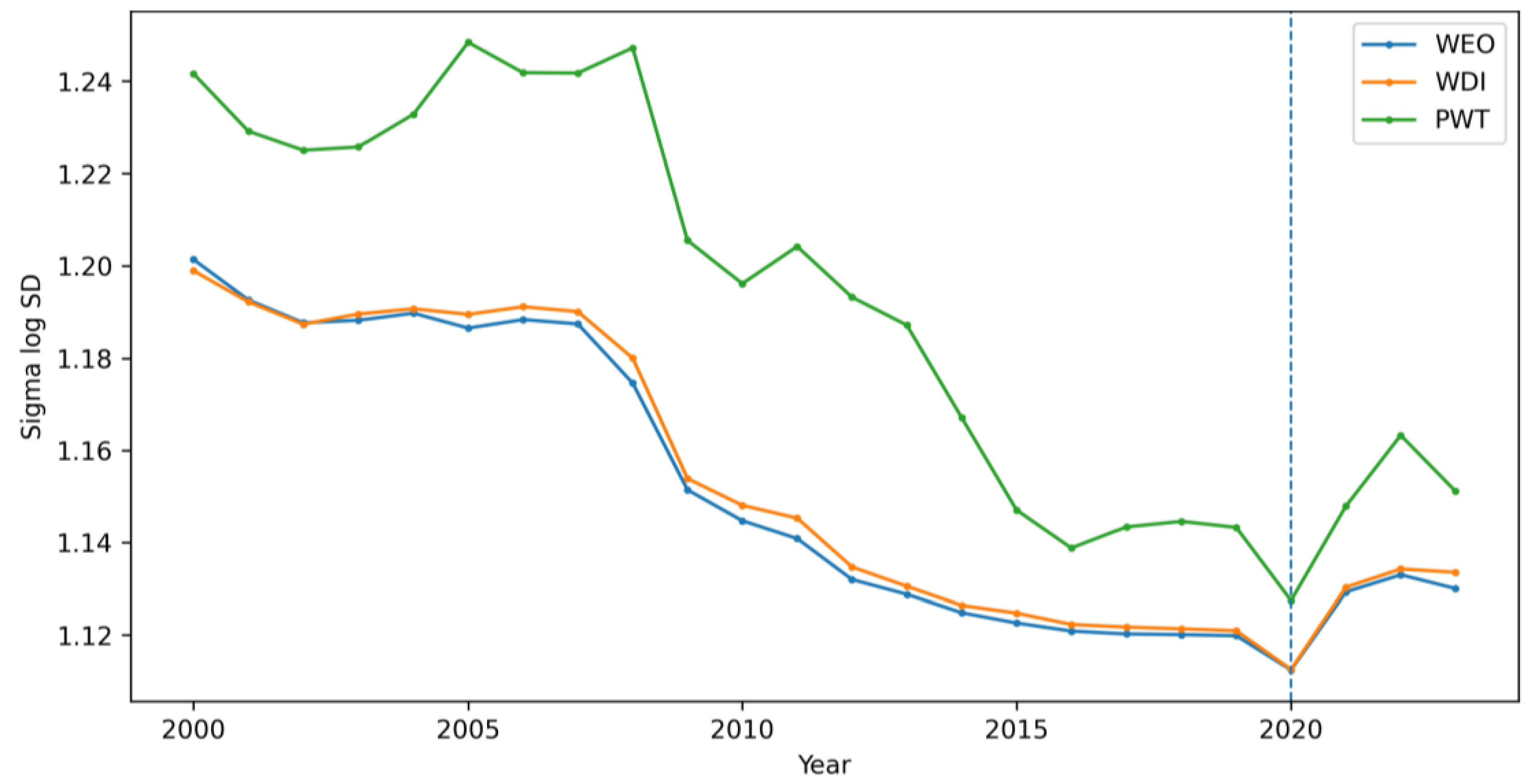
External comparisons use the World Development Indicators (WDI) (World Bank, 2026) and Penn World Table (PWT) 11.0 (Feenstra et al., 2025), with the PWT methodology attributed separately to Feenstra et al. (2015). WDI uses NY.GDP.PCAP.PP.KD and SP.POP.TOTL; PWT GDP per capita is rgdpe/pop. Their feasible terminal years differ, so harmonized comparisons end in 2023. The source windows are consequently distinct: WEO extends provisionally through 2025, WDI through 2024 where available, and PWT through 2023. WDI and PWT do not replace WEO as the principal long-run source. They provide external checks on whether the direction and metric sensitivity of the WEO findings persist under alternative data-construction systems and feasible terminal years. Source-specific magnitudes are not expected to coincide because the series differ in national-account revisions, PPP implementation, real-income concepts, coverage, and extrapolation practices.

To separate source construction from country composition, the analysis retains 167 countries observed in all three sources for every year from 2000 through 2023, yielding 12,024 source-country-year observations. ISO3 codes define matches. Detailed source-specific coverage and exclusions are reported in Appendix A 

Table A2. Harmonized 167-Country Sample Coverage by Source.

Source	Raw Country Count	Complete, 2000–2023	Retained in Common Sample	Dropped
WEO	197	185	167	18
WDI	199	191	167	24
PWT	185	182	167	15

Notes: The harmonized design contains 167 countries observed in all three sources over 2000–2023, corresponding to 12,024 source-country-year observations.

and

Table A3. Dropped-Country Summary by Source and Reason.

Source Dropped from	Reason	N
PWT	Not complete in WDI	3
PWT	Not complete in WEO	5
PWT	Not complete in WEO and WDI	7
WDI	Not complete in PWT	12
WDI	Not complete in WEO	5
WDI	Not complete in WEO and PWT	7
WEO	Not complete in PWT	12
WEO	Not complete in WDI	3
WEO	Not complete in WDI and PWT	3

Notes: Counts summarize 57 source-specific exclusions from the common sample. The complete row-level country list with ISO3 codes is designated for the replication package.

and the replication materials.

Balanced and maximum-coverage samples answer different questions. The fixed WEO panels support historical comparison, while maximum samples preserve broader country coverage. The harmonized panel controls cross-source country and year composition but does not make the three measurement systems conceptually identical.

Table 2. Data Sources and Sample Construction.

Source/Sample	Role	Income Variable	Population Variable	Period	Country Coverage	Notes
IMF WEO April 2026.	Main historical WEO baseline (1980–2024)/ provisional 2025 WEO extension	NGDPRPPPPC: GDPpc PPP, constant 2021 international dollars	LP: population, millions	1980–2024 baseline; 1980–2025 provisional	195 any valid 1980–2025; 138 balanced 1980–2024; 137 balanced 1980–2025	2025 is an IMF estimate/provisional value.
WDI	External comparison and common-sample replication	GDP per capita, PPP, constant international dollars	Population	1990–2024; common sample 2000–2023	199 in WDI panel; 191 complete 2000–2023; 167 common	Country-level metrics, bootstrap, decomposition, concentration, beta, and rank diagnostics.
PWT 11.0	External comparison and common-sample replication	GDP per capita constructed as rgdpe/pop	PWT population: pop	Through 2023; common sample 2000–2023	182 complete 2000–2023; 167 common	PWT limits harmonized post-2020 comparison to 2020–2023.
Harmonized WEO–WDI–PWT sample	Cross-source robustness	Source-specific GDPpc harmonized by ISO3	Source-specific population	2000–2023	167 × 24 × 3 = 12,024 observations	Same countries and years; no duplicate source-country-year keys.

Notes: The main historical WEO baseline (1980–2024) contains 138 balanced countries; the provisional 2025 WEO extension uses a separate 137-country balanced sample over 1980–2025. WDI and PWT are external sources for comparison. WEO 2025 observations are provisional IMF estimates. PWT ends in 2023 in this replication design. Interpretation: The table separates the main WEO evidence from external comparisons and harmonized common-sample robustness checks.

summarizes the variables, periods, and sample roles. Further implementation details and complete country lists are retained in Appendix A and replication outputs rather than repeated in the main text.

3.2. Distributional Measures

Let $y_{i,t}$ denote real GDP per capita at purchasing power parity for country i in year t, and let $x_{i,t}=\ln \left(y_{i,t}\right)$. WEO and WDI supply PPP-adjusted constant-price GDP per capita directly; PWT GDP per capita is constructed as described in Section 3.1. Observations with non-positive income are excluded from calculations requiring logarithms. Population weights are each country’s share of sample-year population:

$$w_{i,t}={\displaystyle \frac{{\mathrm{p}\mathrm{o}\mathrm{p}}_{i,t}}{{\sum }_i{\mathrm{p}\mathrm{o}\mathrm{p}}_{i,t}}}$$

The weights sum to one within each sample-year. Equal-country measures give every economy the same influence; population-weighted Gini and Theil give larger economies greater influence while retaining one country-average income value. They therefore remain between-country measures rather than estimates of global interpersonal inequality.

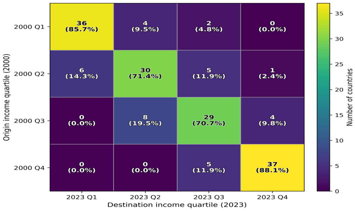
Income-group definitions depend on the diagnostic. Long-run mobility analysis uses fixed initial-year income quartiles: countries are classified once from GDP per capita in the initial year of the relevant sample and are followed under that classification. Benchmark-year transition matrices compare the quartile associated with the initial benchmark to the country’s terminal-year quartile. By contrast, the 2020–2023 variance decomposition in Section 4.4 uses fixed 2020 income quartiles applied to both years. These conventions prevent annual reclassification from obscuring persistence and keep the decomposition groups constant over the post-2020 comparison window.

Relative income is defined, where required, as a country’s GDP per capita divided by the contemporaneous cross-country mean or median: $r_{i,t}={\displaystyle \frac{y_{i,t}}{{\overline{y}}_t}}$, or $r_{i,t}={\displaystyle \frac{y_{i,t}}{{\mathrm{median}}_i\left(y_{i,t}\right)}}$. It is used only as a descriptive distributional diagnostic. Rank measures the order of countries by GDP per capita at selected benchmark years and supports Spearman correlations, transition matrices, same-quartile persistence, and upward or downward quartile movement.

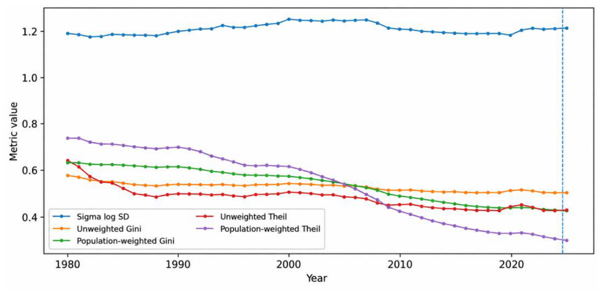
Sigma dispersion is the cross-sectional standard deviation of log GDP per capita. With $x_{i,t}=\ln \left(y_{i,t}\right)$, cross-country mean ${\overline{x}}_t$, and $N_t$ countries in year t, it is defined in Equation (1):

$${\sigma }_t={\left[{\displaystyle \frac{1}{N_t-1}}\sum _i{\left(x_{i,t}-{\overline{x}}_t\right)}^2\right]}^{{\displaystyle \frac{1}{2}}}$$

(1)

A decline in ${\sigma }_t$ denotes sigma convergence and an increase denotes sigma widening. The sample-standard-deviation convention uses denominator $N_t-1$, rather than $N_t$, and the $N_t-1$ convention is applied consistently to the historical series, harmonized comparisons, decomposition, and paired resampling. Equations (1)–(9) and all empirical specifications are otherwise unchanged.

Sigma measures proportional dispersion around the cross-country log-income mean and limits the dominance of extreme level-income observations relative to an untransformed standard deviation. Post-2020 sigma changes are examined in the main historical WEO baseline, the provisional 2025 WEO extension, source-specific WDI and PWT samples over their feasible windows, and the harmonized 167-country panel. This sequence evaluates whether the measured direction is sensitive to a provisional endpoint, source choice, or country coverage without treating the sources as identical.

Gini and Theil indices are computed from country-level GDP per capita because level-income inequality need not move with log-income dispersion. Let ${\mu }_t$ denote the mean GDP per capita across the $N_t$ countries in year t. The unweighted Gini is defined in Equation (2):

$$G_t={\displaystyle \frac{1}{2{N_t}^2{\mu }_t}}\sum _i\sum _j\left|y_{i,t}-y_{j,t}\right|$$

(2)

For population weights $w_{i,t}$ satisfying ${\sum }_i{w}_{i,t}=1$ and weighted mean ${\mu }_t^w={\sum }_i{w}_{i,t}{y}_{i,t}$, the population-weighted Gini is defined in Equation (3):

$$G_t^w={\displaystyle \frac{1}{2{\mu }_t^w}}\sum _i\sum _j{w}_{i,t}{w}_{j,t}\left|y_{i,t}-y_{j,t}\right|$$

(3)

The unweighted Theil index is defined in Equation (4):

$$T_t={\displaystyle \frac{1}{N_t}}\sum _i\left[{\displaystyle \frac{y_{i,t}}{{\mu }_t}}\ln \left({\displaystyle \frac{y_{i,t}}{{\mu }_t}}\right)\right]$$

(4)

The population-weighted Theil index is defined in Equation (5):

$$T_t^w=\sum _i{w}_{i,t}\left[{\displaystyle \frac{y_{i,t}}{{\mu }_t^w}}\ln \left({\displaystyle \frac{y_{i,t}}{{\mu }_t^w}}\right)\right]$$

(5)

The unweighted Gini and Theil measures of unweighted between-country GDP per capita inequality assign equal weight to countries. Their population-weighted counterparts measure population-weighted between-country GDP per capita inequality by weighting the same country-level income values by population shares. Neither specification observes income dispersion within countries. Comparisons among sigma, Gini, and Theil are therefore interpreted as evidence on metric sensitivity: sigma describes log-income spread, while Gini and Theil summarize the level-income distribution under different weighting schemes.

All annual metrics are computed within the country set defined for the relevant specification. Consequently, differences between balanced, maximum-unbalanced, and harmonized results can reflect both the income paths represented and the composition rule. The manuscript reports these designs separately rather than pooling them into one series or treating their levels as directly interchangeable.

Tail diagnostics comprise P90/P10, P75/P25, and the ratio of the mean GDP per capita of the ten highest-income countries to that of the ten lowest-income countries. The first two are $R_{90/10,t}={\displaystyle \frac{\mathrm{P}90\left(y_t\right)}{\mathrm{P}10\left(y_t\right)}}$ and $R_{75/25,t}={\displaystyle \frac{\mathrm{P}75\left(y_t\right)}{\mathrm{P}25\left(y_t\right)}}$. The top10/bottom10 ratio is defined in Equation (6):

$$R_{\mathrm{T}\mathrm{o}\mathrm{p}10/\mathrm{B}\mathrm{o}\mathrm{t}\mathrm{t}\mathrm{o}\mathrm{m}10,t}={\displaystyle \frac{\mathrm{mean}\left(y_{\mathrm{T}\mathrm{o}\mathrm{p}10,t}\right)}{\mathrm{mean}\left(y_{\mathrm{B}\mathrm{o}\mathrm{t}\mathrm{t}\mathrm{o}\mathrm{m}10,t}\right)}}$$

(6)

P90/P10 emphasizes the outer deciles, P75/P25 captures a broader separation around the middle half of the distribution, and top10/bottom10 compares the means of the extreme groups. These measures help distinguish extreme-tail concentration from wider interquartile movement. They remain supplementary because ratios based on distribution tails can be sensitive to small-country observations, source-specific measurement, and exceptionally high incomes; the related sample restrictions are described in Section 3.4.

3.3. Beta-Convergence and Rank-Mobility Diagnostics

Beta convergence is evaluated using descriptive cross-country growth regressions. For country i, annualized log GDP per capita growth between the initial year $t_0$ and terminal year $t_1$ is computed in Equation (7):

$$g_{i,t_0,t_1}={\displaystyle \frac{\ln \left(y_{i,t_1}\right)-\ln \left(y_{i,t_0}\right)}{t_1-t_0}}$$

(7)

The descriptive beta-convergence regression is specified in Equation (8):

$$g_{i,t_0,t_1}=\alpha +\beta \ln \left(y_{i,t_0}\right)+{\epsilon }_i$$

(8)

A negative descriptive beta-convergence coefficient indicates that initially poorer countries grew faster on average during the specified period. A positive coefficient indicates a positive initial-income–growth gradient, while a coefficient closer to zero than in an earlier window indicates attenuation of catching-up. The regressions are estimated for 2000–2023, for the pre-2020 period 2000–2019, and for the short post-2020 window 2020–2023. These windows permit comparison of the full common-sample relationship with the pre- and post-2020 gradients without treating the latter as a structural break estimate.

The specification is unconditional. The coefficients are used as descriptive growth-gradient summaries, with the short 2020–2023 window interpreted cautiously because it may reflect temporary cross-country macroeconomic variation. Heteroskedasticity-robust White/HC1 standard errors are reported. Each regression is a single cross-section of 167 countries rather than repeated observations within clusters, so no natural clustering dimension is available, and no clustering adjustment is applied. R² values of approximately 0.01–0.15 are consistent with a summary growth gradient rather than a fully specified growth model; no conditional-convergence claim is made.

Rank mobility provides a separate test of whether average growth differences correspond to changes in relative position. Spearman’s rank correlation between GDP per capita ranks in initial and terminal benchmark years is defined in Equation (9):

$${\rho }_s=\mathrm{corr}\left[\mathrm{rank}\left(y_{i,t_0}\right),\mathrm{rank}\left(y_{i,t_1}\right)\right]$$

(9)

Higher ${\rho }_s$ indicates greater persistence in the cross-country income ranking, while lower values indicate more extensive reordering. Benchmark-year quartile transition matrices classify countries by initial benchmark-year GDP per capita and record their terminal-year quartile. The matrices yield same-quartile persistence and the shares moving upward or downward by at least one quartile. These diagnostics complement the descriptive beta-convergence regressions because an initially poorer country may grow faster yet remain in the same rank range or quartile when the initial income gap is large; conversely, modest changes near a quartile boundary may produce mobility without a large change in aggregate dispersion.

3.4. Bootstrap, Influence Diagnostics, and Interpretation Boundaries

Sample and source checks combine the balanced historical WEO panel, the separate provisional 2025 extension, the maximum-unbalanced WEO sample, WDI and PWT external comparisons, and the harmonized 167-country panel. Balanced samples maintain fixed composition, the maximum-unbalanced sample preserves wider WEO coverage, and excluding the provisional endpoint tests whether the historical conclusion depends on 2025. The harmonized panel holds countries and years constant across all three sources, while source-specific samples retain their feasible coverage. Appendix A 

Table A4. Maximum- and Common-Sample Metric Changes, 2020–2023.

Source	Sample	N	Δ Sigma	Δ Gini	Δ Theil	Δ Top10/Bottom10
WEO	Maximum	185	+0.0195	−0.0060	−0.0110	+2.4788
WEO	Common	167	+0.0176	−0.0080	−0.0141	+0.5400
WDI	Maximum	191	+0.0339	+0.0007	+0.0013	+6.4748
WDI	Common	167	+0.0210	−0.0061	−0.0102	+2.8582
PWT	Maximum	182	+0.0421	−0.0004	+0.0002	+7.7167
PWT	Common	167	+0.0237	−0.0016	−0.0017	+4.1778

Notes: Maximum samples use each source’s complete available country set for 2000–2023; common-sample rows use identical 167-country coverage. The comparison assesses sensitivity to country composition, not equality of source-specific magnitudes.

compares maximum- and common-sample results. Together, these designs assess sensitivity to terminal-year status, source construction, and country composition without assigning identical interpretation to all samples. Cross-source agreement is evaluated directionally rather than by requiring equal magnitudes. WEO, WDI, and PWT retain differences in PPP benchmarks, national-account revisions, extrapolation, and real GDP concepts even after harmonization. The common sample reduces the possibility that apparent source disagreement is produced only by different countries, whereas remaining discrepancies may reflect measurement-system differences. This role is distinct from the influence and resampling diagnostics applied within a specified country set.

For selected changes, countries are sampled with replacement, with the same resampled country indices applied to both endpoints. The paired statistic summarizes aggregate change under repeated country draws; its interval and positive-resample share describe sign stability, not country breadth. Leave-one-country-out and predefined exclusion checks assess sensitivity to single observations and sample definitions. Paired resampling, additive contributions, and joint exclusion therefore retain distinct estimands.

The interpretation boundary is fixed throughout. The post-2020 period is treated as a descriptive event window rather than an exogenous treatment; decomposition, contribution, exclusion, beta-convergence, rank, and cross-source diagnostics characterize observed distributional patterns rather than identify specific shocks or mechanisms. Unweighted and population-weighted results remain measures of between-country GDP per capita inequality rather than estimates of global interpersonal inequality.

3.5. Historical Magnitude and Concentration Diagnostics

For country $i$ in year t, the additive contribution to the cross-sectional variance of log GDP per capita is defined as

$$c_{it}={\displaystyle \frac{{\left(x_{it}-\overline{x_t}\right)}^2}{N-1}}$$

(10)

where x_it is log GDP per capita, $\overline{x_t}$ is its cross-country mean in year t, and N is the number of countries. The country-specific contribution to the 2020–2023 variance change is

$$\mathsf{\Delta }{c}_i=c_{\mathrm{i},2023}-c_{\mathrm{i},2020}$$

(11)

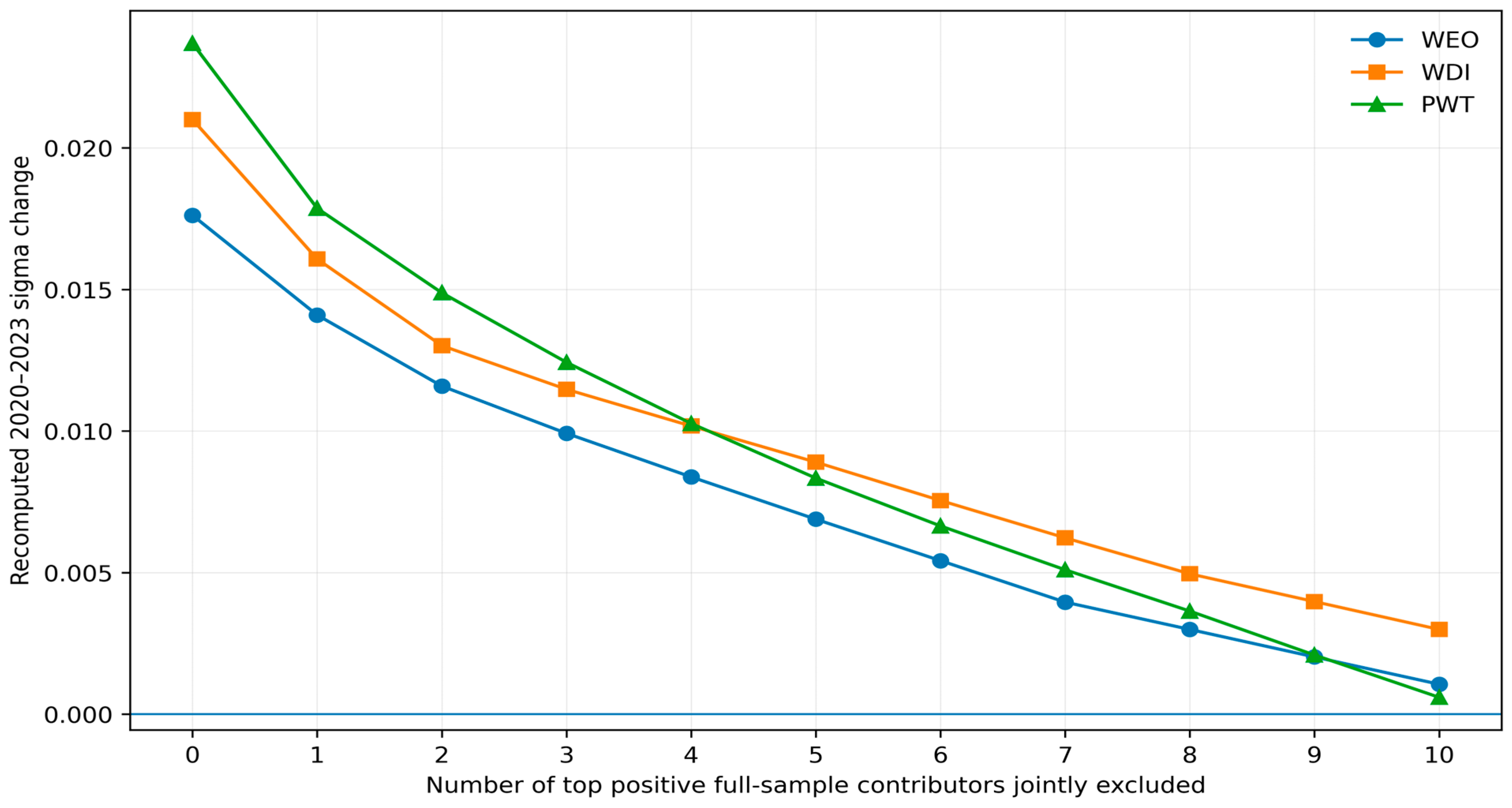
By construction, these country-specific changes sum to the full-sample variance change, subject to machine precision. Top-five and top-ten shares are computed within the original full sample and identify concentration; they do not by themselves describe the recomputed distribution after exclusions.

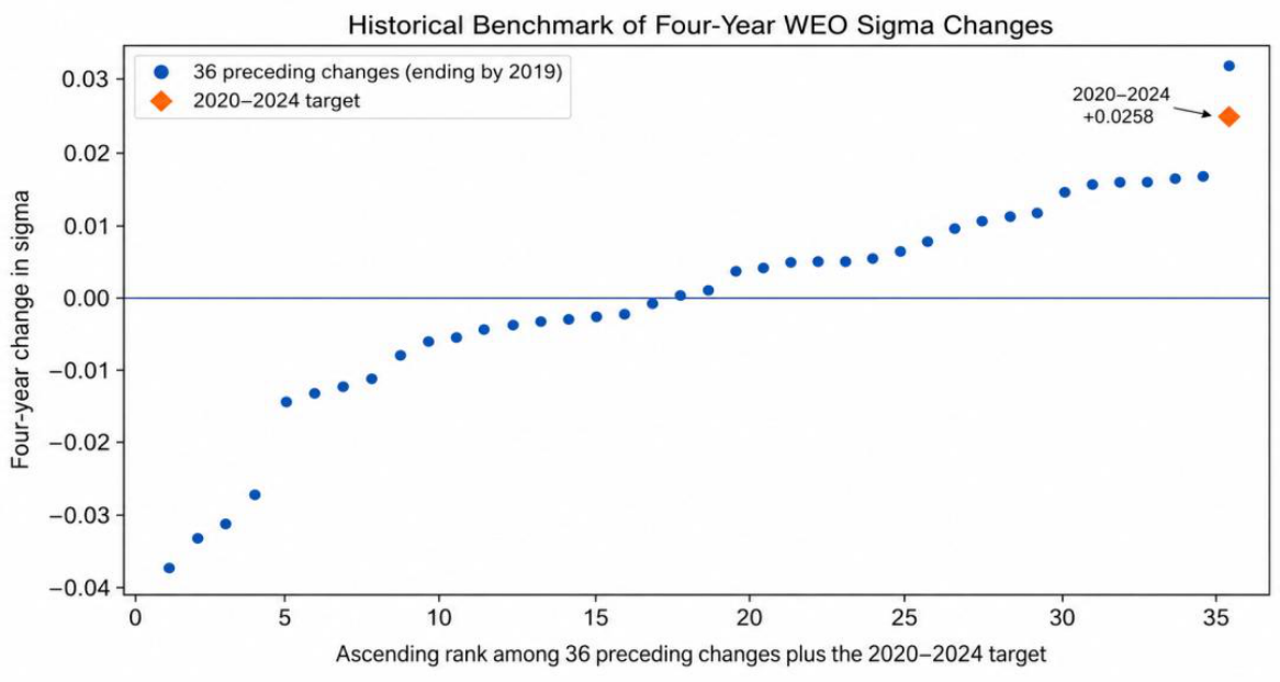
The joint-exclusion exercise ranks countries by positive ${\mathsf{\Delta }\mathrm{c}}_I$ and jointly removes the first k contributors from both endpoints for $k=0,\dots ,10$ recomputing sigma and variance on each remaining sample. Because exclusion changes the mean, sample size, and all deviations, the residual path need not equal one minus the original cumulative contribution share. The exercise is reported as an ex-post concentration stress test. Historical magnitude is assessed with ${\Delta }_4{\sigma }_t={\sigma }_t-{\sigma }_{t-4}$ on the locked 138-country WEO 1980–2024 series. The primary benchmark compares 2020–2024 with the 36 preceding four-year windows ending by 2019; the complete 41-window distribution is supplementary. Because the windows overlap and are serially dependent, ranks and empirical cumulative shares are descriptive and are not interpreted as p-values, confidence intervals, filters, or structural-break tests. Given the short four-to-five-year terminal window, the rolling-window benchmark is used instead of a filtered trend-cycle decomposition, which would introduce additional smoothing, tuning, and endpoint assumptions that the present descriptive design cannot discipline reliably.

4. Results

Results proceed from the long-run WEO series to the harmonized cross-source comparison, historical magnitude, rank persistence, and country-level concentration. The central distinction is between a source-consistent positive aggregate direction and the breadth of country trajectories underlying that change.

4.1. Main Historical WEO Baseline and Provisional 2025 WEO Extension

The long-run WEO series shows high dispersion before 2000, a broad decline through 2019, and a renewed increase after 2020. The recent increase is therefore a short-window movement within a longer convergence history rather than evidence that the long-run path has permanently reversed.

The post-2020 signal is clearest for sigma. Unweighted and population-weighted Gini and Theil move downward or remain approximately flat, so the WEO evidence supports metric-specific log-dispersion widening rather than a general increase across inequality concepts.

Figure 1 displays the fixed 137-country 1980–2025 WEO series, with the provisional 2025 endpoint separated visually. The main historical endpoint comparison remains the 138-country 1980–2024 baseline in

Table 3. WEO Main Metric Changes.

Metric	2020	2024	Change 2020–2024	Provisional 2025 WEO Extension Change
Sigma log SD	1.182	1.208	+0.026	+0.027
Unweighted Gini	0.525	0.516	−0.009	−0.008
Pop-wtd Gini	0.458	0.448	−0.010	−0.013
Unweighted Theil	0.462	0.446	−0.016	−0.015
Pop-wtd Theil	0.360	0.341	−0.019	−0.025
P90/P10	22.38	22.73	+0.350	+0.854
P75/P25	6.56	6.91	+0.352	+0.182
Top10/bottom10	52.70	56.09	+3.393	+4.825

Notes: The 2020–2024 columns report the main historical WEO baseline; the final column reports the separate provisional 2025 extension. Main-table values are rounded for presentation; exact values are retained in the replication outputs.

.

Figure 1 shows that the recent sigma increase follows a longer decline and that Gini and Theil do not share its post-2020 direction. This visual comparison establishes horizon and metric sensitivity but does not determine whether widening is broad across countries. Table 3 reports the principal endpoint changes. In the 138-country historical baseline, sigma rises from 1.1818 in 2020 to 1.2075 in 2024, a change of +0.0258. The separate provisional extension also remains positive through 2025. These changes are already present before the provisional endpoint is added.

The level-based measures move in the opposite direction: unweighted and population-weighted Gini and Theil decline over the reported WEO windows while selected tail ratios increase. Economically, the wedge indicates that proportional distances can widen in log-income space without a corresponding general rise in level-based between-country inequality. Historical calibration further qualifies the result: the 2020–2024 sigma change is exceeded by only two of the 36 preceding four-year changes ending by 2019, yet sigma in 2024 remains 0.03785 below its 2000 level. Figure 2 places the 2020–2024 sigma increase in historical context by comparing it with the 36 preceding four-year changes ending by 2019.

4.2. Cross-Source Common-Sample Evidence

WDI and PWT provide external comparisons under alternative data systems. The strongest comparison holds the same 167 countries and years fixed across WEO, WDI, and PWT, yielding 12,024 source-country-year observations over 2000–2023. Full-sample sigma rises by 0.018 in WEO, 0.021 in WDI, and 0.024 in PWT, so the positive direction is source-consistent despite differences in PPP and national-account construction. Figure 3 illustrates the evolution of sigma across the harmonized WEO, WDI, and PWT sample over 2000–2023.

Table 4. WEO–WDI–PWT Harmonized Common-Sample Results.

Source	Period	Countries	Sigma Change	Gini Change	Pop-Weighted Gini Change	Theil Change	Pop-Weighted Theil Change	Top10/Bottom10 Change
WEO	2020–2023	167	+0.018	−0.008	−0.004	−0.014	−0.009	+0.540
WDI	2020–2023	167	+0.021	−0.006	−0.004	−0.010	−0.009	+2.858
PWT	2020–2023	167	+0.024	−0.002	−0.001	−0.002	−0.004	+4.178

Notes: Harmonized 167-country sample, 2000–2023, 12,024 source-country-year observations. The table uses identical ISO3 countries and years across sources. Magnitudes need not match because WEO, WDI, and PWT use different data construction methods. Interpretation: Sigma increases across all three sources under identical country coverage; Gini and Theil do not indicate a corresponding general increase in between-country inequality across the reported metrics.

places the positive sigma changes beside non-positive or near-zero Gini and Theil changes. Population weighting also does not produce a corresponding increase; economically, movements with substantial equal-country influence do not translate proportionately once countries are weighted by population. The top10/bottom10 ratio rises in all three sources, but its paired resampling intervals include zero, so it remains a supplementary tail diagnostic. Section 4.4 addresses the remaining question of breadth.

4.3. Beta Convergence and Rank Persistence

Table 5. Descriptive Beta-Convergence Regressions.

Source	Period	N	Descriptive Beta-Convergence Coefficient	Std. Error	p-Value	R2	Interpretation
WEO	2000–2023	167	−0.005	0.001	<0.001	0.115	Average catching-up over full common period.
WEO	2000–2019	167	−0.006	0.001	<0.001	0.136	Pre-2020 beta convergence.
WEO	2020–2023	167	+0.004	0.002	0.051	0.013	Descriptive attenuation of pre-2020 catching-up.
WDI	2000–2023	167	−0.005	0.001	<0.001	0.106	Average catching-up over full common period.
WDI	2000–2019	167	−0.006	0.001	<0.001	0.131	Pre-2020 beta convergence.
WDI	2020–2023	167	+0.005	0.002	0.025	0.018	Descriptive attenuation of pre-2020 catching-up.
PWT	2000–2023	167	−0.006	0.001	<0.001	0.140	Average catching-up over full common period.
PWT	2000–2019	167	−0.007	0.001	<0.001	0.154	Pre-2020 beta convergence.
PWT	2020–2023	167	+0.005	0.003	0.068	0.015	Descriptive attenuation of pre-2020 catching-up.

reports the descriptive beta-convergence regressions specified in Section 3.3. They summarize average catching-up patterns under the unconditional specification.

Harmonized 167-country WEO–WDI–PWT sample over 2000–2023. The dependent variable is annualized log GDP per capita growth, and the key regressor is initial log GDP per capita. Coefficients are descriptive growth-gradient summaries; see Section 3.3. Interpretation: beta convergence is visible before 2020, while the short 2020–2023 window shows attenuation.

The temporal pattern is consistent across sources. Over 2000–2023, the descriptive beta-convergence coefficients are negative, ranging from −0.0048 to −0.0061. They are more negative during 2000–2019, ranging from −0.0056 to −0.0071, indicating stronger average catching-up before 2020. Over the short 2020–2023 window, the coefficients become positive, ranging from +0.0037 to +0.0048. These ranges summarize the cross-source pattern without treating small differences in individual estimates as substantively distinct.

Over 2020–2023, the coefficients become positive, ranging from +0.0037 to +0.0048, indicating descriptive attenuation of the earlier catching-up relationship. Given the short window, modest explanatory power, and non-uniform statistical evidence across sources, the estimates are not interpreted as a durable reversal; specification limits are detailed in Section 3.3. This temporal contrast is compatible with the sigma findings. Average catching-up over a long interval concerns the relationship between initial income and subsequent growth, whereas sigma records the cross-sectional dispersion of log income at each date. A negative long-run growth gradient can therefore coexist with renewed short-window dispersion if catching up is uneven, if some initially poorer countries fall back, or if movements at the upper and lower tails offset changes elsewhere in the distribution.

Rank diagnostics assess whether longer-run catching-up produced broad reordering.

Table 6. Rank Persistence and Quartile Mobility.

Source	Period	Countries	Spearman Rank Correlation	Same-Quartile Share	Upward Quartile Share	Downward Quartile Share	Interpretation
WEO	2000–2023	167	0.946	0.790	0.096	0.114	High-rank persistence.
WDI	2000–2023	167	0.948	0.784	0.102	0.114	High-rank persistence.
PWT	2000–2023	167	0.939	0.761	0.120	0.120	High-rank persistence.

Notes: Harmonized 167-country sample over 2000–2023. Initial and terminal quartiles are computed within each source using GDP per capita ranks in the relevant benchmark years. Rank mobility is conceptually distinct from beta convergence. Interpretation: High same-quartile shares indicate persistent income hierarchy and limited mobility.

reports Spearman correlations and quartile transitions; Figure 4 displays the WEO transition matrix. The diagnostics record positional persistence rather than average growth differences.

Spearman correlations range from 0.9391 to 0.9476 across WEO, WDI, and PWT, indicating limited reordering between 2000 and 2023. Same-quartile persistence ranges from 0.7605 to 0.7904. In country counts, approximately 132 WEO countries, 131 WDI countries, and 127 PWT countries remain in their initial quartile out of 167. Upward and downward movements are both limited, and several off-diagonal transition cells contain only small numbers of countries. The transition shares are therefore interpreted descriptively rather than as precise mobility probabilities.

Figure 4 concentrates most observations on the diagonal. Spearman correlations of 0.939–0.948 and same-quartile shares of 0.761–0.790 indicate limited reordering across sources, even though some movement occurs between adjacent quartiles. The longer WEO comparison points in the same direction. Between 1980 and 2025, rank correlation remains high, and 71.4% of countries in the fixed initial-year lowest-income quartile remain in that quartile at the terminal benchmark. Average pre-2020 catching-up can therefore coexist with persistent ranks and limited quartile mobility. Faster growth among initially poorer countries may narrow some proportional gaps without eliminating large starting differences or producing broad upward reordering.

4.4. Concentration, Hierarchy, and Sequential Exclusion

This subsection distinguishes the location of the variance increase from its breadth. It combines the fixed-2020-quartile variance split, additive country contributions, tail-membership stability, and sequential ex post exclusion. These diagnostics characterize concentration but do not formally decompose the difference among sigma, Gini, and Theil. Countries are assigned once to fixed 2020 income quartiles, and the same groups are applied in 2023.

Table 7. Fixed-2020-Quartile Decomposition of Log-Income Variance.

Source	Year	Total Variance of Log GDP p.c.	Between-Quartile Variance	Within-Quartile Variance	Between-Quartile Share
WEO	2020	1.237	1.116	0.122	90.1%
	2023	1.277	1.146	0.131	89.7%
WDI	2020	1.238	1.117	0.121	90.2%
	2023	1.285	1.154	0.131	89.8%
PWT	2020	1.271	1.147	0.124	90.3%
	2023	1.325	1.193	0.133	90.0%

Notes: Quartiles are fixed from 2020 GDP per capita and applied to both years. The split is descriptive and does not identify convergence clubs.

reports the ANOVA-style variance split; higher-precision values are retained in the replication outputs.

Between-quartile variance accounts for about 90% of the variance level and for 77%, 79%, and 84% of the 2020–2023 variance increase in WEO, WDI, and PWT, respectively. The fixed-group result is consistent with persistent ranks: separation can increase among established groups without broad reclassification; the high between-group level share partly reflects defining groups from the income distribution itself. Country-level contributions are changes in squared log deviations from the source-specific mean divided by N − 1.

Table 8. Largest Positive Country Contributions to the 2020–2023 Variance Change.

Source	Rank	Country	Contribution to Change in Log-Income Variance
WEO	1	Sudan	+0.0081
	2	Guyana	+0.0058
	3	Haiti	+0.0039
	4	Burundi	+0.0038
	5	Central African Republic	+0.0034
WDI	1	Sudan	+0.0114
	2	Guyana	+0.0070
	3	Haiti	+0.0037
	4	Central African Republic	+0.0033
	5	Burundi	+0.0031
PWT	1	Sudan	+0.0135
	2	Guyana	+0.0070
	3	Liberia	+0.0059
	4	Qatar	+0.0051
	5	Central African Republic	+0.0046

Notes: Contributions are additive within the original full sample and measure country-level influence on the observed variance change.

reports the five largest positive contributors; the full rankings are retained in the replication outputs.

The concentration is substantial and source-specific. Top-five shares are 63.4% in WEO, 60.3% in WDI, and 66.9% in PWT; top-ten shares are 93.8%, 86.6%, and 96.3%. Sudan and Guyana rank first and second in all three sources, while other rankings differ. Their trajectories also illustrate why external context and data vintage matter: Sudan’s 2023 observation coincides with severe conflict-related economic disruption, whereas Guyana’s recent path coincides with rapid oil-led expansion and national-account rebasing (Bureau of Statistics, Guyana, 2020; United Nations, 2023; World Bank, 2024b, 2024c, 2025). These contexts help explain why the observations merit scrutiny, but they are not interpreted as identified mechanisms.

Table 9. Contributor Concentration and Ex Post Joint-Exclusion Results.

Source	Full Δσ	Top-Five Share	Top-Ten Share	Δσ After Top Five	Δσ After Top Ten	Residual (%)	Pattern
WEO	0.0176	63.4%	93.8%	0.0069	0.0011	6.0%	Near-total
WDI	0.0210	60.3%	86.6%	0.0089	0.0030	14.2%	Strong
PWT	0.0237	66.9%	96.3%	0.0083	0.0006	2.5%	Near-total

Notes: Contribution shares are additive in the original full sample. Joint exclusion recomputes all sample moments and is reported as an ex-post concentration stress test. Exact full-precision values are retained in the replication outputs.

reports the recomputed joint-exclusion results. Removing the top ten positive contributors leaves small positive sigma changes of 0.001056 in WEO, 0.002992 in WDI, and 0.000594 in PWT—6.0%, 14.2%, and 2.5% of the respective full-sample changes. Widening therefore does not disappear, but WEO and PWT are almost entirely concentrated, and WDI is strongly concentrated.

Tail membership is also stable: most 2020 top- and bottom-ten countries remain in the same tail in 2023. The top10/bottom10 changes therefore mainly reflect movements within established extremes rather than wholesale replacement of tail membership.

The sequential exclusion path in Appendix A Figure A1 makes the contraction in recomputed sigma visible for k = 0, …, 10. Because each exclusion changes the mean, sample size, and all deviations, the residual path is not equal to one minus the cumulative additive share.

Taken together, the evidence establishes a positive but concentrated aggregate change superimposed on a persistent hierarchy. Economically, the metric wedge is consistent with sharply differentiated country trajectories at the distributional tails rather than a common deterioration in relative income positions across most economies.

4.5. Results Synthesis

The full-sample sigma direction is positive across WEO, WDI, and PWT, but country breadth is limited. Gini and Theil do not show a corresponding general increase; the historical WEO change is high over a short horizon while the 2024 level remains below 2000; and rank persistence remains strong.

Fixed-quartile and contributor diagnostics show that the positive aggregate signal is concentrated in a few tail trajectories, with only small positive residuals after the top ten are jointly excluded. The defensible synthesis is therefore concentrated, metric-sensitive short-window widening within a persistent hierarchy—not broad-based divergence or a structural break.

5. Robustness and Sensitivity Analysis

5.1. Sample Balance, 2025 Exclusion, and Source Choice

Balanced, maximum-coverage, and harmonized samples retain the positive sigma direction while differing in magnitude. Excluding the provisional 2025 endpoint also leaves the historical WEO change positive. These checks establish sensitivity to coverage and endpoint status; they do not establish broad country breadth.

The historical calibration in Figure 2 provides the relevant short-horizon benchmark: +0.0258 is large relative to preceding four-year changes but remains part of an overlapping, serially dependent sequence and is not a structural-break estimate.

Cross-source agreement under identical coverage strengthens the direction claim. The concentration and exclusion results in Table 9 then show that source consistency and broad-based widening are separate questions.

5.2. Influential Countries, Microstates, and Resource-Economy Sensitivity

Leave-one-country-out results show that no single removal reverses the WEO sign. This is compatible with strong joint concentration because several influential observations can sustain a positive aggregate change even when no one observation is individually decisive. Predefined microstate, resource-economy, and high-income exclusions remain sensitivity checks rather than preferred baselines. Appendix A Figure A1 reports the separately ranked top-one to top-ten joint-exclusion path. Appendix A 

Table A10. WEO Descriptive Beta-Convergence Specification Sensitivity.

Period	Countries	Quartile FE	Beta	HC1 SE	Approx. p-Value	R2
2000–2019	185	No	−0.00533	0.00112	0.0000	0.1114
2000–2019	185	Yes	−0.01067	0.00370	0.0040	0.1695
2020–2024	195	No	+0.00633	0.00219	0.0038	0.0378
2020–2024	195	Yes	+0.00239	0.00665	0.7188	0.1345
2000–2024	185	No	−0.00455	0.00102	0.0000	0.0885
2000–2024	185	Yes	−0.01008	0.00363	0.0056	0.1453
2020–2023	195	No	+0.00728	0.00203	0.0003	0.0474
2020–2023	195	Yes	+0.00341	0.00571	0.5501	0.1352

Notes: The dependent variable is annualized log GDP per capita growth, and the key regressor is initial log GDP per capita. HC1 heteroskedasticity-robust standard errors are reported. Quartile fixed effects are descriptive controls based on fixed initial-year income quartiles and are reported only as a specification-sensitivity check.

adds fixed initial-year income-quartile controls to the descriptive beta-convergence regression as a specification-sensitivity check rather than a structural convergence model.

5.3. Paired Country-Resampling Bootstrap Uncertainty

The WEO-only and harmonized paired country-resampling exercises apply the same resampled country indices to both endpoints.

Table 10. Paired Country-Resampling Bootstrap Results, Harmonized 167-Country Sample, 2020–2023.

Metric	Source	Observed Change, 2020–2023	95% Paired Country-Resampling Bootstrap Interval	Share of Bootstrap Changes > 0
Sigma log SD	WEO	+0.018	[+0.004, +0.032]	0.994
	WDI	+0.021	[+0.007, +0.038]	0.999
	PWT	+0.024	[+0.005, +0.044]	0.995
Unweighted Gini	WEO	−0.008	[−0.014, −0.002]	0.004
	WDI	−0.006	[−0.012, −0.000]	0.020
	PWT	−0.002	[−0.010, +0.007]	0.344
Pop.-weighted Gini	WEO	−0.004	[−0.016, +0.009]	0.358
	WDI	−0.004	[−0.018, +0.009]	0.363
	PWT	−0.001	[−0.014, +0.014]	0.498
Unweighted Theil	WEO	−0.014	[−0.025, −0.003]	0.005
	WDI	−0.010	[−0.021, +0.000]	0.030
	PWT	−0.002	[−0.017, +0.016]	0.402
Pop. -weighted Theil	WEO	−0.009	[−0.027, +0.013]	0.275
	WDI	−0.009	[−0.030, +0.015]	0.302
	PWT	−0.004	[−0.024, +0.023]	0.410
Top10/bottom10 ratio	WEO	+0.540	[−1.890, +3.668]	0.699
	WDI	+2.858	[−0.988, +6.058]	0.908
	PWT	+4.178	[−2.580, +9.823]	0.886

Notes: The same resampled country indices are applied to both endpoint years. Intervals summarize descriptive resampling uncertainty rather than classical random-sampling inference. Sigma intervals exclude zero, and positive-resample shares exceed 0.99 in all three sources, indicating aggregate sign stability under the specified design. This does not imply broad-based country widening because influential observations recur frequently in country resamples. Gini and Theil provide no corresponding positive signal, while top10/bottom10 intervals include zero and remain supplementary.

reports the harmonized 5000-replication results for WEO, WDI, and PWT.

5.4. Robustness Synthesis

The robustness evidence supports a positive aggregate direction across sources, endpoints, and resampling designs, while the exclusion path shows that the increase is not broad-based. Sign stability and country breadth are therefore reported separately.

6. Discussion

6.1. Metric Divergence, Scale, and Weighting

The post-2020 sigma–Gini/Theil wedge is consistent with the broader measurement literature showing that conclusions depend on the statistical object, weighting scheme, and data construction. Anand and Segal (2008) and Atkinson and Brandolini (2001) emphasize sensitivity to measurement choices, while Deaton (2021) shows that pandemic-era between-country conclusions can differ materially under equal-country and population weighting. In the present evidence, sigma rises across WEO, WDI, and PWT even as unweighted and population-weighted Gini and Theil remain flat or decline. Economically, the pattern indicates wider proportional distances in log-income space without a corresponding general deterioration in the level-income distribution. Cross-source agreement is also notable because PPP revisions and alternative macroeconomic data systems can materially change cross-country levels and growth comparisons (Deaton & Heston, 2010; S. Johnson et al., 2013). Harmonizing countries and years does not remove those construction differences, but it reduces sample composition as a competing explanation for disagreement. The weaker response of population-weighted measures further indicates that country trajectories with substantial equal-country influence do not translate proportionately once countries are weighted by population. This remains distinct from global interpersonal inequality analyses that incorporate within-country distributions (Mahler et al., 2022).

6.2. Concentration and Post-2020 Heterogeneity

The concentration evidence qualifies any broad divergence interpretation. The top ten contributors account for 86.6–96.3% of the variance increase, and joint exclusion leaves only 2.5–14.2% of the original sigma change. This is consistent with post-pandemic evidence emphasizing heterogeneous rather than uniform country outcomes (Adarov et al., 2022; Brussevich et al., 2022). The present analysis adds a distributional diagnostic: cross-source sign consistency coexists with highly concentrated country-level influence.

The identities of leading contributors reinforce the need for bounded contextual interpretation. Sudan’s recent trajectory coincides with severe conflict-related economic disruption, whereas Guyana’s trajectory coincides with rapid oil-led output expansion and national-account rebasing (Bureau of Statistics, Guyana, 2020; United Nations, 2023; World Bank, 2024b, 2024c, 2025). These contexts are consistent with unusually large country-level movements, but they are not treated as identified causes of the aggregate sigma change.

6.3. Persistence, Convergence, and Horizon

High rank correlations and limited quartile mobility place the post-2020 change within a persistent hierarchy. This is consistent with distribution-dynamics research emphasizing that average catching-up need not imply extensive reordering of relative income positions (Quah, 1996a, 1996b; Maasoumi et al., 2007). The fixed 2020 quartiles are descriptive partitions rather than estimated convergence clubs, distinguishing this exercise from formal club-convergence approaches such as Phillips and Sul (2007). The historical horizon also matters. The pre-2020 negative growth gradients are compatible with studies documenting stronger cross-country catching-up since the late twentieth century (Patel et al., 2021; Kremer et al., 2022; Lähdemäki, 2024), while the persistent hierarchy remains consistent with P. Johnson and Papageorgiou’s (2020) caution that convergence has been incomplete and uneven. Because the 2020–2024 WEO increase is historically high over a four-year window but sigma in 2024 remains below its 2000 level, the evidence is best read as a concentrated short-horizon departure from earlier narrowing rather than a permanent reversal. Taken together, the literature comparison and empirical diagnostics reconcile the apparent metric tension. Post-2020 proportional distances widened in log-income space, but the broader level-income distribution, especially under population weighting, did not show a corresponding general increase; the widening was concentrated within a durable rank hierarchy. The contribution is therefore an integrated interpretation of scale, weighting, concentration, persistence, and horizon rather than a claim that any single metric provides a complete account of cross-country convergence.

6.4. Limitations and Scope Conditions

The unit of analysis is the country. Population weighting changes country influence but does not recover within-country distributions, so no result is interpreted as global interpersonal inequality.

The design is descriptive and non-causal. Decomposition, contributor ranking, exclusion, beta gradients, and country context locate patterns but do not identify the effects of conflict, oil production, fiscal capacity, productivity, policy, or pandemic shocks.

WEO, WDI, and PWT share national-account and PPP foundations while differing in revisions, coverage, and real-income construction. Harmonization controls composition but not conceptual equivalence. Sudan and Guyana also illustrate why extreme trajectories may be sensitive to data vintage and national-account revisions.

The post-2020 comparison is short, and source endpoints differ. The rolling-window benchmark is descriptive because the windows overlap; it is not a filter, trend decomposition, or structural-break test. Future vintages may alter exact magnitudes, especially the provisional 2025 extension.

7. Conclusions

Across the harmonized 167-country sample, sigma log GDP per capita dispersion increased by 0.018–0.024 between 2020 and 2023 in WEO, WDI, and PWT, while unweighted and population-weighted Gini and Theil showed no corresponding general increase. The widening was strongly concentrated: the top five contributors accounted for 60.3–66.9% of the variance increase and the top ten for 86.6–96.3%, with only small positive residuals after joint exclusion. The WEO 2020–2024 increase was historically high over a four-year horizon, yet sigma in 2024 remained below its 2000 level. The academic contribution is an integrated distribution-diagnostics framework that combines identical-country cross-source comparison with scale, weighting, concentration, persistence, and horizon. It clarifies why sigma, level-based inequality measures, contributor diagnostics, and mobility indicators can provide different but mutually consistent signals. Interpretation is limited by the short post-2020 window, source-specific national-account and PPP construction, the provisional 2025 WEO extension, and the descriptive design. The analysis concerns between-country GDP per capita and does not measure global interpersonal inequality. Future research should test whether the concentrated pattern persists as later WEO, WDI, and PWT vintages mature, examine whether contributor breadth changes over longer horizons, and use channel-specific data and credible identification strategies to study heterogeneous country trajectories. Household-distribution data would be required to connect these between-country patterns to global interpersonal inequality.