Dynamic Wage Adjustment Under Fertility-Policy Regime Transitions: System GMM Evidence from China

Abstract

China’s transition from strict fertility control toward a pronatalist regime raises important questions regarding how institutional regime changes are associated with wage outcomes across different policy stages. While previous studies primarily examine contemporaneous labor-market outcomes, this study evaluates wage associations across fertility-policy regime stages using a dynamic panel specification. Using five waves of the China Family Panel Studies (CFPS) from 2014 to 2022, the analysis constructs a short, unbalanced panel and estimates a wage equation using two-step System Generalized Method of Moments (System GMM) with collapsed instruments and restricted lag depth to address dynamic endogeneity and unobserved heterogeneity. To improve representativeness and mitigate observed wage-observability differences, survey weights are combined with inverse-probability weighting. The preferred baseline estimates indicate a positive but modest lagged-wage coefficient. Monte Carlo and sensitivity analyses further suggest that the persistence estimate is fragile and may overstate the degree of true persistence in this short-panel setting. Accordingly, the findings do not support strong intertemporal wage persistence and instead indicate only limited dependence of current wages on past wage realizations. The dynamic specification is therefore informative primarily as a diagnostic framework for assessing whether regime-stage wage associations exhibit meaningful persistence. Additional exposure-based heterogeneity analyses show negative interaction coefficients for Female and childbearing women (CBW). Married women aged 20–39 experience additional negative wage associations during fertility-policy regime stages, with similar results obtained under a narrower CBW20–35 robustness definition. These findings suggest that positive aggregate regime-stage associations may conceal relative wage disadvantages among women in demographic groups more plausibly exposed to fertility-policy-related labor-market conditions. The CBW indicator is interpreted as a demographic-exposure proxy rather than as a direct measure of employer expectations, fertility intentions, or discrimination. Overall, the results highlight exposure-based heterogeneity in regime-stage wage associations while emphasizing that the estimates should be interpreted as conditional associations embedded within broader institutional transitions rather than as causal fertility-policy effects.

1. Introduction

China’s transition from strict fertility control to a pronatalist policy regime represents a major demographic shift that raises fundamental questions about labor-market adjustment under changing population structures. These policy reforms aim to address the country’s aging population and declining fertility rates, but they may also be associated with unintended labor-market consequences, particularly in relation to gender inequality (Albanesi et al., 2023).

Fertility-policy transitions may reshape employer expectations regarding Female labor-force participation, childbirth, caregiving responsibilities, and career continuity, with potential implications for wages, career advancement, and labor-force attachment (Blau & Kahn, 2017). Existing studies have examined employment and labor-force participation outcomes associated with fertility-policy changes, but longer-term wage dynamics remain less explored. Limited attention has been given to whether wage associations aligned with fertility-policy regime stages persist over time and whether these associations differ across groups more plausibly exposed to fertility-related labor-market expectations.

This study aims to fill this gap by examining how fertility-policy regime transitions are associated with wage dynamics over time, with a particular focus on intertemporal wage adjustment and exposure-based heterogeneity. Using data from the China Family Panel Studies (CFPS) between 2014 and 2022, this paper models wage dynamics through a dynamic wage equation that incorporates lagged wages, policy-stage indicators, and exposure-based interaction terms. Unlike studies that focus primarily on contemporaneous employment outcomes or static wage differences, this study assesses whether wage associations aligned with fertility-policy regime stages display any limited carry-forward through lagged wage dependence and whether more exposed groups experience differential wage associations.

The central question of this paper is therefore twofold. First, are fertility-policy regime transitions associated with wage changes within a dynamic wage structure? Second, do these regime-stage wage associations differ for women more plausibly exposed to fertility-policy-related labor-market expectations? This perspective shifts the analysis from static comparisons of wage levels to the intertemporal adjustment of policy-stage wage associations and the exposure-based heterogeneity embedded in those associations. The dynamic nature of wage adjustment is important because wage persistence determines whether short-run policy-stage associations dissipate or carry forward into longer-run wage implications.

This paper contributes to literature in three ways. First, and most importantly, it foregrounds exposure-based heterogeneity in regime-stage wage associations. Rather than treating fertility-policy regime transitions as producing homogeneous wage associations across all individuals, the analysis distinguishes aggregate policy-stage associations from differential associations among women more plausibly exposed to fertility-policy-related demographic and labor-market expectations. Specifically, this paper compares a broad Female interaction specification with a more targeted CBW specification, where CBW refers to married women aged 20–39; a narrower married-women-aged-20–35 definition is also used as a robustness check.

Second, this paper shows that positive aggregate regime-stage wage associations may conceal negative differential associations for more exposed Female groups. This distinction is important because wave-level policy-stage coefficients may absorb secular wage growth, macroeconomic adjustment, COVID-19-era disruption, and other contemporaneous institutional changes. The exposure-based interaction results, therefore, provide the main empirical basis for interpreting heterogeneity within fertility-policy regime stages, while remaining associational rather than causal.

Third, this paper uses dynamic System GMM specification as a diagnostic framework rather than as the central contribution of the manuscript. The System GMM estimator addresses the presence of a lagged dependent variable and helps assess whether lagged wage dependence materially changes the interpretation of contemporaneous regime-stage wage associations. Because the estimated persistence is modest and unstable across sensitivity checks, the dynamic specification is used to discipline and limit the interpretation of carry-forward, not to claim strong intertemporal wage persistence or substantive long-run policy effects. The empirical implementation combines disciplined instrument selection, survey-consistent weighting, inverse-probability weighting, and MBF-based evidence interpretation in a short and unbalanced CFPS panel.

Previous studies have primarily focused on static treatment-effect frameworks or contemporaneous labor-market outcomes, such as employment, labor-force participation, or wage differences associated with fertility-policy reforms (Albanesi et al., 2023; Blau & Kahn, 2017). In contrast, this study highlights the intertemporal adjustment of policy-stage wage associations and examines whether aggregate policy-stage associations conceal differential wage patterns among women more plausibly exposed to fertility-related labor-market expectations. This perspective redefines how policy-stage wage associations should be interpreted in dynamic labor-market settings.

This study formulates four testable hypotheses based on the theoretical framework and existing literature.

H1. 

Wage persistence, if present, is expected to be limited in the short and unbalanced CFPS panel.

H2. 

Later fertility-policy regime-stage survey waves are positively associated with aggregate wage levels relative to the pre-two-child reference period, after controlling observed individual characteristics and dynamic wage dependence.

H3. 

Policy-stage wage associations may exhibit limited carry-forward through lagged wage dependence.

The purpose of testing H3 is not to impose a large long-run interpretation in advance, but to assess whether the data supports any meaningful carry-forward of policy-stage wage associations after accounting for dynamic endogeneity. The finding of limited persistence is therefore informative because it prevents overstatement of long-run regime-stage wage associations.

H4. 

Exposure-based interaction coefficients for Female and CBW groups differ from the aggregate policy-stage associations, reflecting differential wage associations among women more plausibly exposed to fertility-policy-related labor-market expectations.

These hypotheses provide a structured foundation for evaluating the empirical results and ensuring the replicability of the analysis.

The remainder of this paper is organized as follows. Section 2 reviews the relevant literature on fertility-policy transitions, labor-market outcomes, wage dynamics, and dynamic panel estimation. Section 3 outlines the theoretical framework, empirical specifications, exposure definitions, and System GMM estimation strategy. Section 4 presents empirical results, focusing on baseline regime-stage wage associations, modest dynamic persistence, exposure-based heterogeneity, robustness checks, and weighting-scheme sensitivity. Section 5 discusses the theoretical, methodological, and policy implications of the findings. Section 6 concludes.

2. Literature Review

This section reviews the literature on fertility-policy transitions, wage dynamics, and the econometric challenges associated with modeling persistent wage processes. It highlights the key theoretical mechanisms and identifies the gap that motivates the present study.

2.1. Fertility Policy Transitions and Labor-Market Outcomes

A substantial body of research examines the economic consequences of fertility policies, particularly in economies experiencing demographic transition and declining fertility. Early studies primarily focus on demographic responses, analyzing how fertility regulations affect birth rates, household decisions, and population structure (Angrist & Evans, 1998; Schultz, 2005; Cruces & Galiani, 2007). More recent work extends this perspective to labor-market outcomes, emphasizing employment, labor-force participation, and earnings (Ebenstein, 2010; Dong & Li, 2025; Shen et al., 2024). However, much of the literature remains focused on static, short-term employment effects, providing limited insight into how policy-stage wage associations evolve through the wage process over time (Albanesi et al., 2023). This limitation is particularly important in the presence of wage persistence, where short-run policy-stage wage associations may carry forward into longer-run labor market patterns.

In the Chinese context, fertility-policy reforms represent a sequence of institutional regime changes rather than isolated policy interventions. The transition from the One-Child policy to the Universal Two-Child policy and subsequently to the three-child policy constitutes a major shift in demographic governance. These reforms may not only affect labor supply but could also influence wage-setting behavior and career trajectories (Blau & Kahn, 2017). Existing studies typically examine these reforms through fertility responses or labor-supply adjustments (Dong & Li, 2025; Shen et al., 2024), while evidence on wage outcomes remains comparatively limited. Prior research has documented persistent gender earnings differences in urban China (Démurger et al., 2007), while recent evidence also suggests that fertility-related discrimination may appear in hiring and employer evaluations in China (Li & Xiao, 2025).

From a theoretical perspective, fertility-policy transitions may be linked to wages through multiple channels. Human capital theory suggests that anticipated fertility decisions influence investment in skills, career continuity, and occupational choices (Becker, 1964; Mincer & Polachek, 1974; Blau & Kahn, 2017). At the same time, statistical discrimination models highlight that employers may rely on group-level expectations when individual productivity is imperfectly observed (Phelps, 1972; Arrow, 1973; Altonji & Pierret, 2001; Blau & Kahn, 2017). As policy transitions may alter perceived fertility risks, firms may adjust wage-setting behavior through expectation-based mechanisms (Goldin, 2014; Albanesi et al., 2023). Despite these theoretical insights, most empirical studies treat policy-related wage differences as contemporaneous or short-run outcomes. Taken together, the existing literature suggests that fertility-policy transitions may be linked to wages through expectation-based mechanisms, but their dynamic implications remain insufficiently explored. If fertility-policy transitions are linked to wages through expectation-based mechanisms, an important question is how these associations evolve in the presence of wage persistence.

Recent evidence from China provides empirical support for this expectation-based interpretation. Huang and Jin (2022) show that the Universal Two-Child policy was associated with reductions in women’s employment and labor income, suggesting that fertility-policy relaxation may generate labor-market costs for women rather than uniformly improve their economic outcomes. Firm-level evidence also suggests that fertility-policy relaxation can change how employers evaluate Female employment and its costs (Leng & Kang, 2022). More directly, Li and Xiao (2025) document fertility discrimination in the Chinese labor market using a correspondence study and an employer survey after the three-child policy and extended parental-leave reforms. Their findings show that married women, particularly those without children, receive fewer callbacks and that hiring managers’ preferences are partly related to concerns about maternity leave. These studies support the theoretical view that fertility-policy regime transitions may alter employer expectations regarding childbirth, caregiving responsibilities, and career continuity, especially for women of childbearing age.

2.2. Wage Dynamics and Persistence

If fertility-policy transitions are linked to wages through expectation-based mechanisms, an important question is how these associations evolve in the presence of wage persistence. A central insight from labor economics is that wages are inherently dynamic, with earnings persistence arising from human-capital accumulation, firm-specific learning, and labor-market matching (Parent, 2002; Meghir & Pistaferri, 2004). Empirical evidence often shows that wages may exhibit serial dependence, although the magnitude of persistence varies across datasets and institutional settings (Meghir & Pistaferri, 2004). Consequently, an empirical question is whether policy-stage wage associations display any meaningful carry-forward through the wage process and, if so, whether such persistence is economically important.

In dynamic settings, short-run wage shifts may have implications extending beyond the contemporaneous period when wages follow autoregressive processes, particularly when demographic policy stages coincide with broader institutional changes in the labor market. This implies that wage changes associated with fertility-policy stages may carry forward across periods, although the magnitude of such carry-forward depends on the estimated persistence parameter (Parent, 2002; Meghir & Pistaferri, 2004). As a result, analyses based on static models may not fully capture whether policy-stage wage associations exhibit any persistence over time.

However, much of the empirical literature continues to rely on static treatment-effect frameworks, such as difference-in-differences approaches, which emphasize contemporaneous effects rather than intertemporal persistence (Angrist & Pischke, 2009; Goodman-Bacon, 2021). The interaction between policy-stage wage shifts and wage persistence remains insufficiently understood.

2.3. Dynamic Panel Estimation and Identification Challenges

Estimating dynamic wage equations presents several econometric challenges. The inclusion of lagged dependent variables introduces endogeneity in the presence of unobserved individual heterogeneity, leading to bias in standard estimators (Nickell, 1981; Arellano & Bond, 1991; Blundell & Bond, 1998). These issues are particularly severe in short and unbalanced panels, where traditional estimators such as fixed effects may yield inconsistent results (Arellano & Bond, 1991).

Generalized Method of Moments (GMM) estimators provide a widely used solution. The difference GMM approach uses lagged levels as instruments, while System GMM improves efficiency by combining equations in differences and levels, addressing endogeneity more effectively (Blundell & Bond, 1998). However, practical implementation requires careful instrument design, as excessive instruments may weaken inference and introduce bias (Roodman, 2009).

Another important issue is sample selection and survey design. Wage observations are often non-random due to labor-force participation and reporting behavior, and large-scale surveys like CFPS involve complex sampling structures. Ignoring these features may lead to biased estimates and reduced external validity, particularly in panel data settings (Heckman, 1979; Deaton, 1997; Wooldridge, 2010). This study integrates survey weights and inverse probability weighting to account for these issues, ensuring more reliable estimates of policy-stage associations.

2.4. Literature Gap and Positioning of the Present Study

Taking together, the existing literature points to a fundamental gap in understanding how fertility-policy regime transitions interact with wage persistence to shape labor-market outcomes over time. While prior studies have examined either the effects of fertility policies or the dynamics of wage persistence, few integrate these two dimensions into a unified analytical framework.

As a result, the intertemporal adjustment of policy-stage wage associations remains insufficiently understood, particularly in settings where wages exhibit persistence and policy changes occur at the institutional level. This limitation is important because it affects how policy-stage associations are interpreted: without accounting for dynamic persistence, short-run associations may misrepresent the longer-run wage patterns aligned with policy shifts.

This study addresses this gap by modeling fertility-related carry-forward associations as institutional regime-stage indicators embedded within a dynamic wage process. By combining dynamic panel estimation with survey-consistent weighting, the analysis assesses whether regime-stage wage associations exhibit any empirically meaningful carry-forward through lagged wage dependence. The results suggest that such carry-forward is weak, fragile, and limited. Rather than treating the findings as evidence of strong intertemporal persistence, the results instead suggest limited intertemporal carry-forward within institutional wage-transition periods. This perspective shifts the analysis from static policy evaluation toward intertemporal institutional wage adjustment within labor markets.

3. Model and Data

3.1. Model Specification and Identification Strategy

Before presenting the model, it is important to clarify the empirical objective and identification boundary of this paper. The present study does not define a treatment group and a control group in the DID sense, nor does it attempt to recover a counterfactual Female wage path in the absence of fertility-policy reform. Instead, it models how wave-level fertility-policy regime indicators enter a persistent wage process and how regime-stage wage associations evolve within a dynamic panel framework.

A central limitation is that the policy-stage variables are defined at the survey-wave level. As a result, the estimated twochild and threechild coefficients cannot be fully separated from secular wage growth, macroeconomic shocks, COVID-19-era labor-market disruption, or other institutional changes occurring during the same periods. Full-time fixed effects cannot be included because they would be perfectly collinear with the wave-level policy-stage indicators. Therefore, the coefficients should be interpreted as conditional regime-stage wage associations rather than causal fertility-policy effects.

The empirical strategy uses System GMM to address dynamic endogeneity arising from the lagged dependent variable and to examine whether regime-stage wage associations carry forward through the wage process. However, the dynamic specification does not solve the time-confounding problem created by wave-level policy coding. The exposure-based Female and CBW interaction specifications help examine differential wage associations among more plausibly exposed groups, but they also remain associational because exposure status is not randomly assigned. This identification boundary is maintained throughout the empirical analysis, discussion, and conclusion.

To avoid overstating the empirical design, the interpretation of the estimates follows a strict hierarchy throughout the paper. First, the aggregate twochild and threechild coefficients are interpreted only as broad wave-level regime-stage wage associations, not as identifiable fertility-policy effects. These coefficients may combine fertility-policy regime timing with secular wage growth, macroeconomic shocks, COVID-19-era disruption, sample-composition changes, and other contemporaneous institutional changes. Second, the Female and CBW interaction terms are interpreted as differential regime-stage wage associations for groups more plausibly exposed to fertility-related labor-market expectations, rather than as causal heterogeneous treatment effects. Third, the adjustment factor is used only as a diagnostic calculation to assess whether contemporaneous regime-stage wage associations carry forward through lagged wage dependence. It is not used to support large long-run causal policy claims. This interpretation hierarchy is maintained in the results, discussion, limitations, and conclusion.

3.1.1. Economic Motivation and Dynamic Wage Specification

China’s transition from strict fertility control to a pronatalist policy regime represents a major institutional shift with potential implications for wage determination. The central objective of this study is to examine how fertility-policy regime transitions enter the wage process and whether the associated wage shifts carry forward to a limited extent within a dynamic earnings structure.

From an economic perspective, fertility-policy transitions may be linked to wages through expectation-based adjustment mechanisms under demographic uncertainty. Changes in fertility policy may reshape expectations regarding childbearing, labor-force attachment, and career continuity, thereby affecting individual human-capital investment and labor-supply decisions. At the same time, firms may update expectations about workforce stability and anticipated labor costs, leading to adjustments in wage-setting behavior. These expectation-based responses provide a theoretical mechanism linking fertility-policy transitions to wage dynamics (Becker, 1964; Mincer & Polachek, 1974; Phelps, 1972; Arrow, 1973; Goldin, 2014). When wages exhibit persistence, these wage adjustments are not necessarily confined to a single period but may persist to a limited extent over time within the dynamic wage process.

A key implication of this mechanism is that policy-stage wage associations may not be purely contemporaneous. If wages are persistent, wage shifts observed in one period may carry forward into subsequent periods through the wage process itself. To capture this dynamic structure, the analysis begins with a baseline dynamic wage specification:

$$\log (wag{e}_{it})=\alpha \log (wag{e}_{i,t-1})+{\beta }_1{\mathrm{twochild}}_t+{\beta }_2{\mathrm{threechild}}_t+X_{it}^{\prime }\gamma +{\mu }_i+{\epsilon }_{it}$$

(1)

where $\log (wag{e}_{i,t})$ denotes the logarithm of hourly wages, $\log (wag{e}_{i,t-1})$ captures wage persistence, and $X_{it}$ is a vector of observed covariates. The parameter $\alpha$ measures the degree of persistence in wages, while ${\beta }_1$ and ${\beta }_2$ capture the average wage associations corresponding to the two-child and three-child policy stages. Because Equation (1) is dynamic, the wage associations linked to regime-stage indicators may remain partially persistent beyond the contemporaneous period through persistence in the wage process. Because the model includes a lagged dependent variable, a mechanical carry-forward calculation can be obtained from the estimated persistence parameter. For a policy-stage coefficient ${\beta }_j$, this diagnostic calculation is written as

$$M{C}_j=\frac{{\beta }_j}{1-\alpha }, j\in \{1,2\}$$

(2)

where $M{C}_j$ denotes a mechanically adjusted association, not a substantively interpretable long-run policy effect. This calculation is reported only to assess whether the estimated lagged-wage dependence would materially change the contemporaneous regime-stage associations. Given the weak and unstable persistence documented in the empirical results, this multiplier should be interpreted as a diagnostic arithmetic transformation rather than as evidence of a meaningful long-run wage effect.

The motivation for employing a dynamic panel framework does not depend on the presence of strong persistence. Rather, the dynamic specification is warranted because current wages may remain partially dependent on past wage realizations, making static estimators potentially biased in the presence of lagged dependent variables and unobserved heterogeneity (Nickell, 1981; Arellano & Bond, 1991; Blundell & Bond, 1998). From this perspective, the empirical contribution of the dynamic framework is diagnostic. It allows the analysis to evaluate whether the estimated wage process displays meaningful persistence. In the present empirical setting, the evidence indicates only modest persistence and limited intertemporal carry-forward.

While Equation (1) captures aggregate wage responses, it implicitly assumes that policy-stage associations are homogeneous across individuals. However, this assumption may be restrictive in the context of fertility-policy reforms. A large body of literature suggests that fertility-related policies may affect men and women differently due to differences in caregiving responsibilities, labor-force attachment, and employer expectations (Becker, 1964; Mincer & Polachek, 1974; Blau & Kahn, 2017; Albanesi et al., 2023).

Employers may update expectations about Female labor supply and potential career interruptions following fertility-policy transitions, leading to differential wage adjustments across gender groups. As a result, the aggregate associations captured by ${\beta }_1$ and ${\beta }_2$ may mask important heterogeneity in wage responses. To account for this, the baseline specification is extended to allow for gender-specific policy-stage associations through interaction terms:

$$\begin{array}{ll}\log (wag{e}_{it})=& \alpha \log (wag{e}_{i,t-1})+{\beta }_{1}twochil{d}_t+{\beta }_{2}threechil{d}_t+\delta femal{e}_i\\ & +{\theta }_1(femal{e}_i\times twochil{d}_t)+{\theta }_2(femal{e}_i\times threechil{d}_t)+X_{it}\gamma +{\mu }_i+{\epsilon }_{it}\end{array}$$

(3)

Equation (3) extends the baseline model by introducing a broad gender-based exposure specification. In this model, $femal{e}_i$ interacts with the policy-stage indicators to examine whether wage associations during fertility-policy regime stages differ between women and other individuals. The interaction terms $femal{e}_i\times twochil{d}_t$ and $femal{e}_i\times threechil{d}_t$ capture additional wage associations for women during the two-child and three-child policy stages, respectively.

However, $femal{e}_i$ is a broad exposure definition. Not all women are equally likely to experience fertility-policy-related expectation shifts. Older women, unmarried women, or women outside the main childbearing and family-formation ages may not face the same employer expectations regarding childbirth, caregiving responsibilities, or career interruptions. Therefore, the Female-interaction specification is useful as a broad gender-based heterogeneity test, but it may not provide the most targeted measure of fertility-policy exposure.

To introduce a more targeted demographic-exposure proxy, this study further constructs a childbearing-women indicator, $CB{W}_i$. The preferred definition is married women aged 20–39, while a narrower definition, married women aged 20–35, is used as a robustness check. These variables are not intended to directly measure fertility intentions, employer expectations, maternity-related discrimination, or actual childbirth behavior. Rather, they identify demographic groups for whom fertility-policy-related labor-market conditions may be more relevant, based on age and marital status. The preferred $CBW$ exposure-proxy specification is written as

$$\begin{array}{ll}\log (wag{e}_{it})=& \alpha \log (wag{e}_{i,t-1})+{\beta }_{1}twochil{d}_t+{\beta }_{2}threechil{d}_t +\\ & {\theta }_1(CB{W}_i\times twochil{d}_t)+{\theta }_2(CB{W}_i\times threechil{d}_t)+X_{it}^{\prime }\gamma +{\mu }_i+{\epsilon }_{it}\end{array}$$

(4)

In Equation (4), ${\theta }_1$ and ${\theta }_2$ capture additional regime-stage wage associations for the $CBW$ demographic-exposure proxy during the two-child and three-child policy stages, relative to other individuals observed in the same policy stages. Compared with the broad Female interaction model, the $CBW$ specification introduces a more targeted demographic grouping. However, it should be interpreted only as a proxy-based heterogeneity specification. It does not directly identify employer expectations, fertility intentions, discrimination, or causal exposure to fertility-policy reform.

This specification does not transform the analysis into a fully causal difference-in-differences design because the policy-stage indicators remain defined at the wave level, and exposure is not randomly assigned. However, it improves the empirical credibility of the analysis by introducing cross-sectional exposure variation through $CB{W}_i\times Polic{y}_t$ interaction terms. This helps distinguish aggregate regime-stage wage associations from differential wage associations among women more plausibly exposed to fertility-policy-related labor-market expectations.

3.1.2. Dynamic Endogeneity and Identification Strategy

The inclusion of the lagged dependent variable in Equations (1), (3) and (4) introduces dynamic endogeneity, as it is correlated with unobserved individual-specific effects. In short panels, fixed-effects estimators are biased (Nickell, 1981), while pooled OLS fails to control unobserved heterogeneity. These issues are particularly relevant in the present context, where the panel is short and unbalanced.

Because the policy-stage indicators vary at the wave level, they do not generate a DID-style treatment contrast within each period. Accordingly, identification in this paper comes from disciplined dynamic-panel variation rather than from a parallel-trends counterfactual design. An important methodological constraint is that full-time fixed effects cannot be included in the specification because they would be perfectly collinear with wave-level fertility-policy regime indicators. This collinearity prevents the separate identification of full-time effects and policy-stage indicators.

Because the policy-stage variables are defined at the wave level, the empirical framework cannot fully disentangle fertility-policy-stage associations from broader macroeconomic and institutional changes occurring during the same periods. This is the central identification limitation of the study. The estimated twochild and threechild coefficients may partly reflect secular wage growth, COVID-19-era labor-market disruption, structural labor-market changes, and other contemporaneous institutional shifts. Accordingly, the estimates should be interpreted as dynamic regime-stage wage associations embedded within broader institutional transitions rather than isolated causal policy effects.

The purpose of the analysis is therefore not to establish a quasi-experimental treatment effect, but rather to examine how policy-stage institutional environments are associated with wage dynamics and exposure-based heterogeneity within a persistent wage process. This interpretation framework is maintained consistently throughout the empirical analysis and discussion sections.

To address concerns regarding omitted macroeconomic shocks, wage growth, COVID-19 impacts, and other time-varying aggregate factors, the robustness analysis later introduces linear time trends, regional time trends, and partial time controls that do not induce perfect collinearity. These exercises are used to assess whether the documented dynamic associations are sensitive to alternative ways of controlling for aggregate time variation. They do not fully eliminate concerns about unobserved macroeconomic shocks, and therefore, the estimates remain interpreted as regime-stage wage associations rather than causal policy effects.

To address dynamic endogeneity, the empirical strategy employs the System Generalized Method of Moments (System GMM), which combines equations in first differences and levels (Arellano & Bond, 1991; Blundell & Bond, 1998). The estimator exploits moment conditions based on lagged values of the dependent variable, under the assumption that the error term is not serially correlated beyond first order. These moment conditions require lagged wages to be correlated with current wages but orthogonal to the contemporaneous error term.

The first-differenced form of the model can be written as

$$\begin{array}{ll}\Delta \log (wag{e}_{it})=& \alpha \Delta \log (wag{e}_{i,t-1})+{\beta }_1\Delta twochil{d}_t+{\beta }_2\Delta threechil{d}_t\\ & +{\theta }_1\Delta (E_i\times twochil{d}_t)+{\theta }_2\Delta (E_i\times threechil{d}_t)+\gamma \Delta X_{it}^{\prime }+\Delta {\epsilon }_{it}\end{array}$$

(5)

where $E_i$ denotes the exposure indicator used in the extended specifications, including $femal{e}_i$, $CBW20-{39}_i$, and $CBW20-{35}_i$. Because these exposure indicators are time-invariant, their main effects are eliminated in first differences, while their interactions with policy-stage indicators remain time-varying through changes in the policy-stage variables.

Because individual-specific effects are eliminated through differencing, identification of the persistence parameter relies on valid internal instruments derived from lagged values of the dependent variable. In this setting, the relevant variation comes from intertemporal changes in lagged wages across individuals, conditional on observed covariates and the maintained moment assumptions. The validity of this strategy depends on the absence of higher-order serial correlation in the idiosyncratic error term and on the appropriateness of the chosen instrument set.

This study relies on three maintained assumptions for System GMM estimation. First, the idiosyncratic error term should not exhibit second-order serial correlation, which is assessed using the Arellano–Bond AR(2) test (Arellano & Bond, 1991). Second, the internal instruments should satisfy the overidentifying restrictions, which are assessed using the Hansen test (Blundell & Bond, 1998). Third, severe omitted time-varying confounding should be limited after conditioning on individual controls and after examining alternative time-related specifications. This third assumption is assessed through robustness checks rather than conclusively verified.

These assumptions allow the dynamic panel model to estimate conditional intertemporal associations within the maintained System GMM framework. They do not by themselves establish causal identification. To reduce weak-instrument and overfitting concerns in the short and unbalanced panel, the preferred baseline specification uses collapsed GMM-style instruments based on lags 1–3 of the lagged dependent variable, whereas the exposure-based heterogeneity and weighting-comparison specifications use the more restrictive lag range of 2–3. This specification-specific instrument design is intended to limit instrument proliferation while retaining sufficient instrument relevance in the short-panel setting (Roodman, 2009). In all reported specifications, the number of instruments remains below the number of panel individuals to reduce overfitting risk. All empirical analyses were conducted in Stata 18. Dynamic panel estimations were implemented using the xtabond2 command with collapsed instruments and Windmeijer-corrected standard errors.

The policy-stage variables ($twochil{d}_t$ and $threechil{d}_t$) are defined at the wave level and treated as exogenous institutional variables. Their coefficients are therefore identified from variation across policy stages, conditional on observed covariates and individual-specific effects. Substantively, these coefficients should be interpreted as regime-stage wage associations within a dynamic framework rather than as individual-level causal treatment effects.

In the broader conceptual specification, interaction terms between gender and policy-stage indicators may also be considered to capture potential heterogeneous responses. Since gender is time-invariant, its main effect is eliminated in first differences, while interaction terms vary over time through the policy-stage variables. In the extended exposure-based specifications, interaction terms between policy-stage indicators and exposure-group indicators are included to examine differential regime-stage wage associations. The Female interaction provides a broad gender-based heterogeneity check, while the CBW interaction introduces a more targeted fertility-exposure definition. Because these interaction specifications remain based on wave-level policy indicators and non-random exposure status, they are interpreted as differential regime-stage associations rather than causal heterogeneous treatment effects.

To ensure reliable inference, instrument proliferation is controlled through collapsed instruments and restricted lag depth (Roodman, 2009). This approach balances instrument relevance and parsimony, reducing the risk of overfitting and weak-instrument bias that can arise in short panel settings. Two-step estimation is implemented with finite-sample corrected standard errors (Windmeijer, 2005), balancing efficiency and robustness. Overall, the System GMM framework is used as a disciplined dynamic-panel estimator under maintained moment assumptions, rather than as a design that solves the wave-level identification problem. Its role is to address dynamic endogeneity from the lagged dependent variable and to assess whether lagged wage dependence materially affects the interpretation of regime-stage wage associations. The estimator therefore supports a cautious dynamic interpretation, but it does not establish causal fertility-policy effects or eliminate time confounding.

3.1.3. Weighting, Wage Observability, and Composite Weights

The CFPS is a complex multi-stage survey, and wage observations are not available for all individuals in all periods. Wage data are observed only when individuals are employed and report valid labor income and working hours. As a result, the estimation sample may be subject to non-random selection, which can lead to biased estimates in the dynamic wage equation.

This issue is particularly important in the context of the dynamic and exposure-based specifications, where wage persistence, policy-stage associations, and interaction-based differential associations are estimated. If wage observability is systematically related to individual characteristics or labor-market conditions, ignoring selection may bias the estimated persistence parameter $\alpha$, as well as the policy coefficients ${\beta }_1$ and ${\beta }_2$, and the interaction-based associations ${\theta }_1$ and ${\theta }_2$.

To address these concerns, the empirical strategy combines survey weights with inverse-probability weighting (IPW). The purpose of this combined weighting strategy is to improve representativeness and to mitigate observed wage-observability differences associated with employment and reporting behavior. The final composite weight is defined as

$$w_{final,it}=w_{svy,it}\times w_{ipw,c,it}$$

(6)

where $w_{svy,it}$ denotes the CFPS survey weight and $w_{ipw,c,it}$ is a stabilized inverse-probability weight.

The probability of observing a valid wage is modeled as $Pr(S_{it}=1\mid Z_{it})=\Lambda (Z_{it}^{\prime }\delta )$ where $S_{it}$ is an indicator for wage observability, and $Z_{it}$ is a set of observed covariates affecting employment and reporting behavior. This selection mechanism reflects the fact that wage observations are conditional on employment and reporting behavior, which may be systematically related to individual characteristics. The predicted probability is given by ${\widehat{p}}_{it}=Pr(S_{it}=1\mid Z_{it})$, and the stabilized inverse-probability weight is constructed as $w_{IPW,it}={\overline{p}}_t/{\widehat{p}}_{it}$ where ${\overline{p}}_t$ denotes the average predicted probability in period t, serving as a stabilizing factor.

This weighting scheme gives higher weight to observations with a lower predicted probability of wage observability and therefore mitigates observable selection associated with employment and reporting behavior. In the empirical implementation, the composite weights are incorporated into descriptive statistics and regression estimation to improve comparability between the descriptive sample and the estimated dynamic wage model (Heckman, 1979; Deaton, 1997; Wooldridge, 2007, 2010). The IPW component should be interpreted as an adjustment for observed wage-observability differences, conditional on the covariates included in the selection model. It is not correct for unobserved selection, nor does it redefine the standard System GMM moment conditions. Accordingly, the weighting strategy is treated as a pragmatic sensitivity and representativeness adjustment rather than as a source of causal identification.

The IPW selection model is estimated using a survey-weighted logit including survey-wave indicators, such as Female, age, age squared, years of education, and urban residence, to predict the probability of observing valid wage information. Stabilized weights are constructed to reduce variance, and the final composite weight is defined as the product of the survey weight and the stabilized IPW weight. This approach mitigates observed wage-observability differences and improves representativeness, but it does not correct for unobserved selection. The weighting strategy is therefore implemented primarily as a pragmatic finite-sample adjustment for survey design and observed wage observability, rather than as a fully design-based GMM framework or a source of causal identification.

3.1.4. Evidence Interpretation: MBF-Based Inference

This study employs Minimum Bayes Factors (MBF) to evaluate statistical evidence, as proposed by Goodman (1999) and Sellke et al. (2001). MBF provides an upper bound on the Bayes factor associated with a given p-value and offers a conservative interpretation of statistical strength, reducing the risk of overstating evidence against the null hypothesis. For practical interpretation, MBF values are calibrated as follows: MBF < 0.1 indicates strong evidence against the null; 0.1 ≤ MBF < 0.3 indicates moderate evidence; MBF ≥ 0.3 indicates weak or no evidence. This approach ensures transparent and disciplined inference and is reported alongside conventional diagnostic statistics for comparability with the existing literature. The notation MBF_SBB refers to the Minimum Bayes Factor calibrated following the Sellke–Bayarri–Berger approach (Sellke et al., 2001).

3.2. Data, Sample Construction, and Variable Measurement

3.2.1. Data Source and Panel Structure

The empirical analysis is based on data from the China Family Panel Studies (CFPS), a nationally representative longitudinal survey covering multiple waves between 2010 and 2022. To ensure consistency in wage measurement and to accommodate the dynamic and exposure-based specifications, the estimation sample is constructed using the waves 2014, 2016, 2018, 2020, and 2022. This period is selected to capture the key fertility-policy regime transitions while ensuring consistency in wage measurements across survey waves.

The requirement of a lagged dependent variable implies that only individuals observed in consecutive waves can be included, resulting in a short and unbalanced panel. This panel structure directly motivates the use of a dynamic panel estimator with disciplined instrument selection, as discussed in Section 3.1.

3.2.2. Wage Construction and Transformations

The dependent variable in all dynamic wage specifications is the logarithm of hourly wages. Hourly wages are constructed from annual labor income and working-time information, following standard survey-based procedures. Specifically, annual working hours are computed as weekly working hours multiplied by 52, and hourly wages are defined as annual labor income divided by annual working hours. This construction ensures comparability across individuals and time, providing a consistent measure of wage outcomes for dynamic analysis.

To ensure comparability across waves and consistency with the logarithmic transformation, observations with non-positive income or invalid working-time information are excluded. These restrictions ensure that the wage variable is well defined and comparable across the estimation sample.

3.2.3. Policy-Regime Coding

The key policy-stage variables used across the dynamic wage specifications are constructed as wave-level policy-stage indicators. These variables capture the institutional environment associated with fertility-policy regimes rather than individual treatment status. Specifically, $twochil{d}_t$ it is defined as an indicator for observations corresponding to the stabilized two-child policy stage, while $threechil{d}_t$ represents the three-child policy regime. This stage-based coding reflects the interpretation of fertility-policy transitions as macro-level institutional shifts that affect the wage-setting environment across all individuals.

This choice necessarily limits the interpretation of the policy-stage coefficients: they summarize wage shifts aligned with institutional regime stages but may also absorb broader time-related changes occurring in the same periods.

Because these policy variables are defined at the wave level, the empirical specification does not include a full set of time-fixed effects, which would otherwise be collinear with the regime-stage indicators. In this context, the regime-stage indicators are designed to capture institutional phase variation that would otherwise be absorbed by time fixed effects, allowing the analysis to focus on policy-aligned temporal shifts in the wage process. This approach is consistent with the identification strategy outlined in Section 3.1, where policy-stage variation is used to capture institutional changes in the wage process.

Accordingly, the regime-stage indicators are interpreted as capturing institutional-phase effects rather than isolated causal impacts of specific policy changes. In the empirical results, their estimated coefficients are therefore discussed as regime-stage wage associations within a dynamic specification, rather than as clean individual-level causal policy associations. Policy-stage indicators are constructed according to the available CFPS survey waves and the observed timing of China’s fertility-policy regime transitions. In the empirical coding used in this study, the pre-two-child reference period covers the earlier CFPS waves before the stabilized two-child Phase II stage. The variable twochild equals one for the 2018 and 2020 survey waves and zero otherwise, capturing the latter two-child policy stage observed in the CFPS panel. The variable threechild equals one for the 2022 survey wave and zero otherwise, corresponding to the survey wave after the announcement of the three-child policy (National Health Commission, 2021). Therefore, the policy-stage variables should be understood as wave-level regime-stage indicators in the CFPS panel rather than as individual-level treatment indicators.

Because these variables vary at the wave level, they are common to all individuals observed in the same survey wave. This coding captures institutional regime-stage timing but does not distinguish individual exposure by marital status, fertility intentions, age, occupation, or gender. Accordingly, the estimated coefficients are interpreted as aggregate regime-stage wage associations rather than individual-level causal treatment effects. The discussion of more exposed groups is used to clarify the theoretical mechanism and the interpretation of possible subgroup patterns, while more sharply identified causal exposure-specific estimates, such as DID/DDD designs with clearer treatment-control contrasts, are left for future research.

In addition to the wave-level policy-stage indicators, the revised analysis constructs exposure variables for heterogeneity analysis. The first exposure variable is ${\mathrm{f}\mathrm{e}\mathrm{m}\mathrm{a}\mathrm{l}\mathrm{e}}_i$, which captures broad gender-based exposure. The second and preferred exposure variable is $CBW20–{39}_i$, defined as married women aged 20–39. This variable is used as a demographic-exposure proxy based on age and marital status. It does not directly measure fertility intentions, actual childbirth plans, employer expectations, maternity-related discrimination, or caregiving responsibilities. Instead, it identifies a demographic group for whom fertility-policy-related labor-market conditions may be more relevant than for the full Female population.

To examine whether the results are sensitive to the age-band definition, a narrower exposure variable, $CBW20–{35}_i$, defined as married women aged 20–35, is also used as a robustness check. The empirical analysis, therefore, distinguishes four specifications: the baseline aggregate policy-stage model, the broad Female interaction model, the preferred CBW20–39 interaction model, and the narrower CBW20–35 robustness model. This structure allows the analysis to separate aggregate regime-stage wage associations from more targeted fertility-exposure patterns.

3.2.4. Core Covariates and Interaction Terms

The vector $X_{it}$ in Equation (1) includes standard demographic and socioeconomic controls, including age, age squared, years of education, and urban residence. These variables account for observable determinants of wages and improve estimation precision. In the exposure-based specifications, the analysis additionally constructs interaction terms between policy-stage indicators and exposure-group indicators. The Female interaction terms capture broad gender-based differential wage associations, while the CBW interaction terms provide a more targeted demographic-exposure proxy for married women of childbearing age.

Specifically, $CBW20–39$ is defined as married women aged 20–39, and $CBW20–35$ is used as a narrower robustness definition. The corresponding interaction terms, Female × $twochild$, Female × $threechild$, $CBW20–39$ × $twochild$, $CBW20–39$ × $threechild$, $CBW20–35$ × $twochild$, and $CBW20–35$ × $threechild$, are used to examine whether aggregate policy-stage wage associations conceal differential associations among women more plausibly exposed to fertility-policy-related labor-market expectations. These interaction coefficients are interpreted as differential regime-stage wage associations rather than causal heterogeneous treatment effects. They should not be interpreted as direct evidence of employer expectations, fertility intentions, or discrimination.

Table 1. Variable definitions and construction (CFPS 2014–2022).

Variable	Definition	Type	Notes/Construction
$\log (wag{e}_{it})$	Log hourly wage	Continuous	Natural logarithm of hourly wage. The hourly wage is calculated as annual labor income divided by annual working hours.
$\log (wag{e}_{i,t-1})$	Lagged log hourly wage	Continuous	One-wave lag of log hourly wage based on the biennial CFPS panel structure.
$twochil{d}_t$	Two-child policy stage	Dummy	Equals 1 for observations in the stabilized two-child Phase II stage, corresponding to the 2018 and 2020 CFPS waves; 0 otherwise.
$threechil{d}_t$	Three-child policy stage	Dummy	Equals 1 for observations in the 2022 CFPS wave after the announcement of the three-child policy; 0 otherwise.
$ag{e}_{it}$	Age	Continuous	Respondent’s age in years.
$ag{e}_{it}^2$	Age squared	Continuous	Squared age terms are used to capture the non-linear life-cycle wage profile.
$educatio{n}_{it}$	Years of education	Continuous	Harmonized years of completed schooling.
$urba{n}_{it}$	Urban residence	Dummy	Equals 1 if the respondent resides in an urban area; 0 otherwise.
$femal{e}_i$	Female indicator	Dummy	Equals 1 for women and 0 for men. Used as a broad gender-based exposure indicator.
$CBW20–{39}_i$	Childbearing women’s exposure group, ages 20–39	Dummy	Equals 1 for married women aged 20–39; 0 otherwise. This is the preferred fertility-exposure definition.
$CBW20–{35}_i$	Narrower childbearing-women exposure group, ages 20–35	Dummy	Equals 1 for married women aged 20–35; 0 otherwise. Used as a narrower robustness exposure definition.
$femal{e}_i$ × $twochil{d}_t$	Female exposure during the two-child stage	Interaction	Interaction between the Female indicator and the two-child policy-stage indicator. Captures additional wage associations for women during the two-child stage.
$femal{e}_i$ × $threechil{d}_t$	Female exposure during the three-child stage	Interaction	Interaction between the Female indicator and the three-child policy-stage indicator. Captures additional wage associations for women during the three-child stage.
$CBW20–{39}_i$ × $twochil{d}_t$	CBW20–39 exposure during the two-child stage	Interaction	Interaction between the preferred CBW20–39 exposure indicator and the two-child policy-stage indicator. Captures additional wage associations for married women aged 20–39 during the two-child stage.
$CBW20–{39}_i$ × $threechil{d}_t$	CBW20–39 exposure during the three-child stage	Interaction	Interaction between the preferred CBW20–39 exposure indicator and the three-child policy-stage indicator. Captures additional wage associations for married women aged 20–39 during the three-child stage.
$CBW20–{35}_i$ × $twochil{d}_t$	CBW20–35 exposure during the two-child stage	Interaction	Interaction between the narrower CBW20–35 exposure indicator and the two-child policy-stage indicator. Used as a robustness interaction.
$CBW20–{35}_i$ × $threechil{d}_t$	CBW20–35 exposure during the three-child stage	Interaction	Interaction between the narrower CBW20–35 exposure indicator and the three-child policy-stage indicator. Used as a robustness interaction.
$w_{final,it}$	Composite probability weight	Continuous	CFPS survey weight multiplied by the stabilized inverse-probability weight. Used to account for complex survey design and non-random wage observability.

Notes: Hourly wage is defined as annual labor income divided by annual working hours, where annual working hours are calculated as weekly working hours × 52. Observations are restricted to individuals with positive labor income and valid working-time information. Policy-stage indicators are coded according to available CFPS survey waves and should be interpreted as wave-level regime-stage indicators rather than individual-level treatment indicators. $CBW20–{39}_i$ denotes married women aged 20–39 and is used as the preferred fertility-exposure definition; $CBW20–{35}_i$ denotes married women aged 20–35 and is used as a narrower robustness definition. Interaction terms are interpreted as differential regime-stage wage associations rather than causal heterogeneous treatment effects. Source: Author’s construction based on CFPS.

reports the definitions and construction of all variables used in the empirical analysis. The notation in the model corresponds directly to the variables used in the dataset, thereby ensuring consistency between the econometric specification and the empirical implementation.

3.2.5. Sample Construction and Estimation-Sample Reconciliation

Because the descriptive analysis, preferred baseline model, exposure-based heterogeneity checks, and weighting-sensitivity analysis impose different data requirements, the reported samples are not a single mechanically nested sequence.

Table 2. Sample construction and estimation-sample reconciliation.

Analytical Sample	Main Sample Requirements	Observations	Individuals/Panel Groups	Source Waves and Effective Estimation Periods	Purpose
Descriptive wage sample	Positive annual labor income and working hours; valid survey and inverse-probability weights; nonnegative education coding; log hourly wage restricted to the range [−2, 8]; one observation per person-wave	33,372	18,061	Source waves: 2014, 2016, 2018, 2020, and 2022	Describes the distribution of wages, policy-stage indicators, and control variables using the composite-weighted descriptive sample
Preferred composite-weighted dynamic-panel sample	Valid current and lagged log hourly wages, controls, survey weights, and stabilized inverse-probability weights; observations must contribute to the preferred two-step System GMM specification	10,035	6138	Source waves: 2014–2022; effective dependent-variable observations arise from 2016 to 2022 because the 2014 wave supplies initial lagged-wage information	Estimates the preferred baseline policy-stage associations; supplies the coefficient inputs for the mechanical carry-forward calculation and the preferred-model diagnostic tests
Exposure-based heterogeneity sample	Valid current and lagged wages, controls, and Female, CBW20–39, or CBW20–35 exposure indicators; does not impose the stricter common-weighting requirement	12,712	7763	Source waves: 2014–2022; effective dynamic estimation uses the available adjacent-wave lag structure	Examines differential policy-stage wage associations for broad and targeted demographic- exposure groups
Restricted common weighting-comparison sample	Observations must be usable under the unweighted, survey-weighted, and composite survey-IPW specifications on exactly the same observations and individuals	8964	5503	Same five source waves and available adjacent-wave lag structure	Isolates sensitivity to alternative weighting schemes while holding the estimation sample fixed

Notes: Observations refer to person-wave records, and individuals refer to unique person identifiers used as panel groups. All empirical samples are drawn from the five CFPS source waves for 2014, 2016, 2018, 2020, and 2022. Because the dynamic specifications include lagged log hourly wage, the effective dependent variable observations begin in 2016, while the 2014 observations provide initial lagged-wage information where available. The samples reported in this table are model-specific analytical samples rather than a single strictly nested sequence. Source: Author’s calculations based on CFPS.

therefore reconciles the analytical samples used across the reported tables. The descriptive sample requires valid wage and weighting information but does not require a lagged wage. The preferred composite-weighted System GMM model additionally requires valid lagged wages, controls, and composite survey-IPW weights. The exposure-based heterogeneity checks use a broader dynamic-panel sample with valid lagged wages, controls, and exposure indicators, while the weighting-scheme comparison uses a stricter common sample that is usable under all three weighting specifications. These model-specific requirements explain the differences in observations and panel groups across tables.

3.2.6. Conceptual Framework

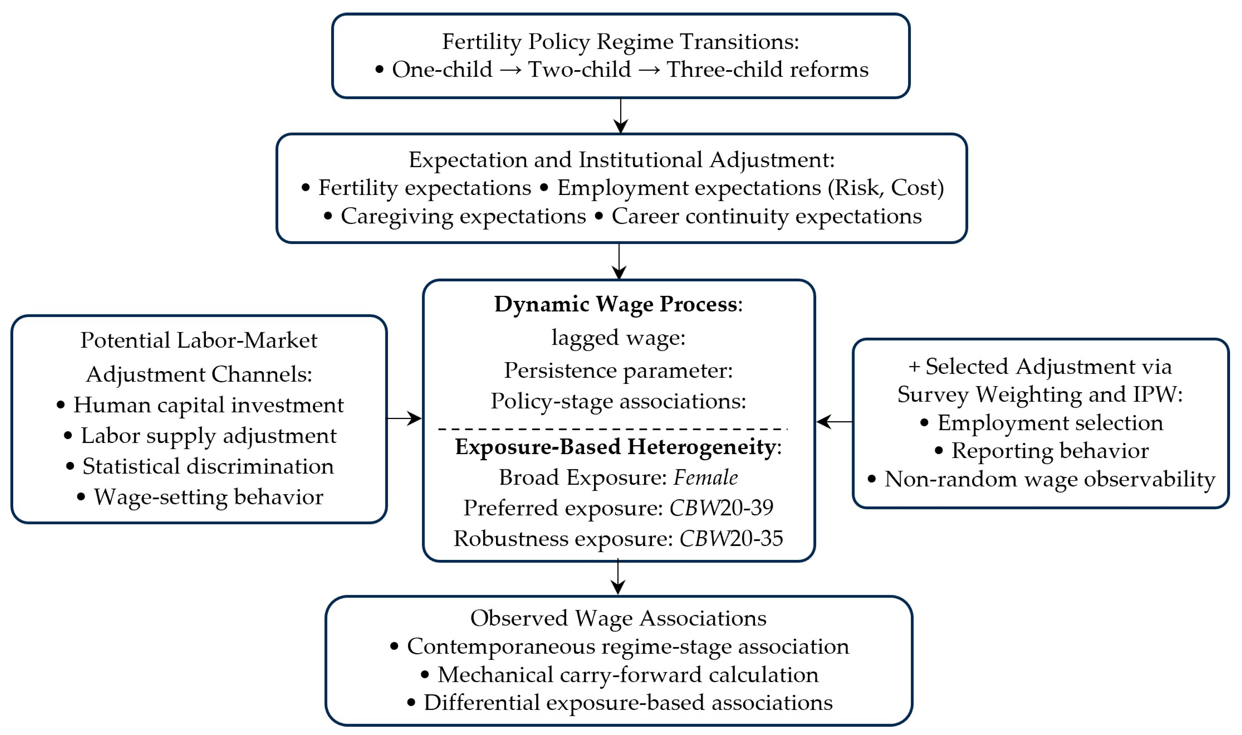
Figure 1 presents the conceptual framework linking fertility-policy regime transitions to dynamic wage associations. Policy-stage changes are theoretically connected to labor-market behavior through expectation-based and institutional mechanisms, including fertility expectations, caregiving expectations, career-continuity concerns, and employer cost or risk expectations. These mechanisms may influence human-capital investment, labor-supply adjustment, statistical discrimination, and wage-setting behavior.

The framework also incorporates a dynamic wage process in which current wages depend partly on lagged wages. This structure allows policy-stage wage associations to operate not only contemporaneously but also through limited intertemporal persistence. Therefore, short-run regime-stage wage associations may exhibit limited carry-forward beyond the contemporaneous period.

In response to the concern that wave-level policy-stage indicators may absorb aggregate time variation, the revised framework explicitly incorporates exposure-based heterogeneity. The broad exposure definition is Female, while the preferred targeted exposure definition is CBW20–39, defined as married women aged 20–39. A narrower CBW20–35 group is used as a robustness exposure definition. These exposure channels motivate the Female × Policy and CBW × Policy interaction specifications used in the empirical analysis.

Finally, the framework accounts for selection into wage observability through survey weighting and inverse-probability weighting. This adjustment is used to mitigate observed wage-observability differences related to employment selection and reporting behavior.

3.2.7. Descriptive Statistics

The descriptive statistics reported in

Table 3. Descriptive statistics (composite-weighted sample).

Variable	Mean (${\mathit{w}}_{\mathbf{f}\mathbf{i}\mathbf{n}\mathbf{a}\mathbf{l}}$)	SD (${\mathit{w}}_{\mathbf{f}\mathbf{i}\mathbf{n}\mathbf{a}\mathbf{l}}$)	Min	Max
Log hourly wage (${lnw}_{\mathrm{i}\mathrm{t}}$)	2.1649	1.0572	−1.985	7.824
Two-child Phase II (2018–2020)	0.1449	0.3521	0	1
Three-child (2022)	0.1209	0.3260	0	1
Age	42.6447	14.1928	14	87
Education (years)	9.5204	4.2115	0	22
Urban	0.5684	0.4953	0	1

Notes: Policy-stage indicators are coded according to CFPS survey waves. The pre-two-child period serves as the reference category, two-child equals one for the 2018 and 2020 survey waves, while threechild equals one for the 2022 survey wave. These variables are wave-level regime-stage indicators and should not be interpreted as individual-level treatment indicators.

are constructed using the same estimation sample as the baseline regression analysis. The sample is restricted to individuals who are employed and report valid labor income and working hours, so that hourly wages can be consistently defined. Observations with missing or non-positive income or invalid working-time information are excluded before constructing the logarithmic wage measure. These restrictions ensure that the descriptive statistics correspond to the same estimation sample used in the dynamic wage analysis.

All descriptive statistics are computed using the composite weight $w_{final,it}$, defined as $w_{final,it}=w_{svy,it}\times w_{ipw,c,it}$, where $w_{svy,it}$ denotes the CFPS survey weight and $w_{ipw,c,it}$ denotes the stabilized and controlled inverse-probability weight that adjusts for non-random wage observability and panel attrition. This composite weight combines the CFPS survey weight with the stabilized inverse-probability weight. The survey-weight component accounts for the CFPS sampling design, while the stabilized IPW component is used to mitigate observed wage-observability differences associated with employment and reporting behavior. The weighting procedure is therefore used to improve comparability between the descriptive sample and the estimated model, not to correct for unobserved selection.

This approach improves consistency between the descriptive statistics and the econometric specification. The reported means, standard deviations, and distributions reflect the same sample restrictions, variable definitions, and weighting structure used in the dynamic wage estimation. Accordingly, Table 3 provides a weighted summary of the estimation sample underlying the empirical analysis.

The descriptive statistics in Table 3 are computed using the same estimation sample and composite weighting scheme as the baseline dynamic specification. The sample includes individuals with valid labor income and working-time information, ensuring that the log hourly wage is well defined. All statistics are weighted using $w_{final,it}=w_{svy,it}\times w_{ipw,it},$ which combines the survey weight with the stabilized IPW component to account for survey design and mitigate observed wage-observability differences.

The mean log hourly wage is approximately 2.16, with substantial dispersion (SD ≈ 1.06), indicating sufficient heterogeneity for identifying wage persistence and policy-stage associations. The policy-stage indicators show that about 14.5% of observations fall in the two-child regime and 12.1% in the three-child regime, providing the time variation needed to identify ${\beta }_1$ and ${\beta }_2$. The sample has an average age of 42.6 years and an average education of 9.5 years, with 56.8% residing in urban areas. These characteristics reflect a diverse working-age population and support the inclusion of standard controls in the wage equation.

4. Results

4.1. Monte Carlo Simulation Results

The purpose of this simulation is to evaluate the performance and limitations of alternative estimators under conditions that mirror the empirical setting, particularly with respect to dynamic persistence, policy-stage variation, and non-random wage observability. The simulation is not intended to validate a strong persistence claim. Instead, it is used to examine how alternative estimators behave in a short and unbalanced panel when the true persistence parameter is small. The true persistence parameter (α) used in the simulation is set to 0.10, which is close to the empirical estimate of 0.0865 and represents a low-persistence data-generating process.

The modest persistence estimate should therefore be interpreted cautiously. The Monte Carlo results indicate that System GMM may still overestimate persistence in short panels when the true persistence parameter is small. Since the empirical estimate is slightly below the simulated true value of 0.10, the possibility that true wage persistence is even weaker cannot be ruled out. This comparison means that the empirical persistence estimate should be treated as a fragile and possibly upper-bound indication of wage persistence in this short-panel setting. If System GMM tends to overestimate persistence when the true parameter is small, and the empirical estimate remains below the simulated benchmark, then the true degree of wage persistence in the empirical data may be close to zero. This possibility is directly incorporated into the interpretation of the results. The dynamic framework is therefore not relied upon to establish a large longer-run wage effect. Instead, it is retained to test whether lagged wage dependence materially changes the interpretation of regime-stage wage associations. The evidence indicates that it does not: any carry-forward is weak, specification-sensitive, and economically limited. This implication does not undermine the revised interpretation of the paper; rather, it reinforces the conclusion that the carry-forward component is limited and that the dynamic framework should not be read as evidence of strong intertemporal wage persistence.

4.1.1. Simulation Design

The simulation uses a five-period balanced-panel benchmark with 6000 individuals and 500 replications. It does not simulate panel attrition, wage-observability selection, or inverse-probability weighting. Its purpose is limited to comparing fixed effects, pooled OLS, and System GMM under a controlled low-persistence dynamic data-generating process. The simulation should therefore be interpreted as an estimator-performance benchmark rather than a full replication of the unbalanced CFPS empirical setting.

Wages are generated following a dynamic process in which current wages depend on past realizations, reflecting the persistence parameter. Policy-stage variables are introduced as time-varying institutional indicators that capture regime shifts across survey waves.

To reflect key features of the empirical data, the simulation incorporates non-random wage observability through a probabilistic selection mechanism linked to employment participation and reporting behavior, consistent with standard sample-selection frameworks (Heckman, 1979; Wooldridge, 2010). Inverse-probability weights are constructed based on predicted observability, mirroring the empirical weighting strategy described in Section 3.

The simulation is conducted under a short and unbalanced panel structure consistent with the CFPS data. Multiple replications are performed to evaluate estimator performance in terms of bias, dispersion, and accuracy. The estimation procedure follows the dynamic panel approach outlined in Section 3, including the use of System GMM to address dynamic endogeneity (Arellano & Bond, 1991; Blundell & Bond, 1998).

4.1.2. Simulation Results

Table 4. Monte Carlo performance of alternative estimators under the dynamic wage model.

Estimator (Parameter)	Bias	MSE (RMSE)	MAPE (%)
FE (alpha)	−0.2994	0.0897 (0.2995)	299.44
FE (threechild)	−0.0351	0.0016 (0.0398)	4.43
FE (twochild)	−0.1182	0.0142 (0.1193)	23.64
OLS (alpha)	0.1871	0.0351 (0.1872)	187.09
OLS (threechild)	0.0229	0.0009 (0.0298)	3.12
OLS (twochild)	0.0747	0.0059 (0.0766)	14.94
SysGMM (alpha)	0.1047	0.0111 (0.1052)	104.72
SysGMM (threechild)	0.0416	0.0021 (0.0460)	5.22
SysGMM (twochild)	0.0556	0.0034 (0.0581)	11.12

Note: Results are based on 500 Monte Carlo replications using a CFPS-like short unbalanced panel. Reported metrics include bias, mean squared error (MSE), root mean squared error (RMSE), and mean absolute percentage error (MAPE).

reports the performance of alternative estimators across key parameters, including the persistence parameter and policy-stage associations. Estimator accuracy is evaluated using bias, mean squared error (MSE), root mean squared error (RMSE), and mean absolute percentage error (MAPE) based on 500 simulation replications. Several clear patterns emerge. First, the fixed-effects estimator exhibits substantial downward bias in the persistence parameter. The estimated bias for $\alpha$ is −0.2994, with an RMSE of 0.2995, confirming the severity of dynamic panel bias in short panels (Nickell, 1981). In contrast, pooled OLS produces an upward-biased estimate of persistence, with a bias of 0.1871 and RMSE of 0.1872, reflecting its inability to control unobserved heterogeneity.

Second, the System GMM estimator improves performance relative to fixed effects and pooled OLS, but the improvement should be interpreted cautiously. The bias in α is 0.1047, with an RMSE of 0.1052. Although this represents better performance than the fixed-effects and pooled OLS estimators, it also shows that System GMM may overestimate persistence when the true parameter is small. This result is consistent with the use of internal instruments to reduce dynamic endogeneity concerns in short panels, but it does not imply that the persistence estimate should be interpreted as strong evidence of intertemporal persistence (Arellano & Bond, 1991; Blundell & Bond, 1998). Third, for policy-stage coefficients, the fixed-effects estimator tends to underestimate the simulated regime-stage associations, while pooled OLS tends to overestimate them. For example, in the case of the two-child policy, fixed effects produce a bias of −0.1182 (RMSE = 0.1193), whereas pooled OLS yields a bias of 0.0747 (RMSE = 0.0766). By contrast, System GMM reduces the bias to 0.0556 with an RMSE of 0.0581, suggesting lower bias for the simulated regime-stage coefficients in this specific design.

A similar pattern is observed for the three-child policy variable. Fixed effects and pooled OLS exhibit smaller but still noticeable biases (−0.0351 and 0.0229, respectively), while System GMM produces a bias of 0.0416 with an RMSE of 0.0460. Although differences are less pronounced for this parameter, System GMM performs relatively better for the simulated regime-stage coefficients in this design, but this result should not be interpreted as a validation of the empirical persistence estimate.

It is also important to interpret MAPE values with caution. For the persistence parameter, MAPE is relatively large across estimators (e.g., 299.44% for fixed effects and 104.72% for System GMM), reflecting the sensitivity of ratio-based measures when estimation errors are large relative to the true parameter. Therefore, bias and RMSE provide more reliable indicators of estimator performance.

These findings show that standard estimators may produce biased results in this setting, which supports the use of a dynamic panel framework when a lagged dependent variable is included. At the same time, the simulation does not provide unconditional validation of System GMM. The upward bias in the simulated persistence estimate indicates that System GMM may still overstate persistence in short panels when the true α is small.

Overall, the simulation results support a cautious use of System GMM rather than a strong persistence interpretation. System GMM performs better than fixed effects and pooled OLS in this simulation design, but it may still overestimate persistence. This finding reinforces the interpretation that the empirical persistence estimate should be treated as positive but modest, and that the implied limited carry-forward should be viewed as limited. Therefore, the Monte Carlo evidence is used to justify a disciplined estimator choice under dynamic endogeneity and to motivate cautious interpretation, not to claim large longer-run wage effects.

4.2. Empirical Results

This subsection presents empirical results from the CFPS dynamic-panel analysis. Consistent with the identification strategy outlined in Section 3, the estimates are interpreted as conditional regime-stage wage associations rather than causal fertility-policy effects. The empirical presentation is organized around two purposes. The first and main purpose is to examine whether aggregate regime-stage wage associations conceal differential associations among more plausibly exposed Female groups. This exposure-based heterogeneity analysis provides the main empirical contribution of the paper.

The second purpose is diagnostic. Because the model includes lagged log wages, the System GMM specification is used to address dynamic endogeneity and to evaluate whether lagged wage dependence materially changes the interpretation of contemporaneous regime-stage associations. This diagnostic use is motivated by the well-known bias of pooled OLS and fixed-effects estimators in short dynamic panels with lagged dependent variables (Nickell, 1981; Arellano & Bond, 1991; Blundell & Bond, 1998). The dynamic component is therefore not treated as the central contribution. Instead, it is used to discipline the interpretation of persistence and carry-forward. As shown below, the estimated persistence parameter is modest and unstable across weighting schemes, so the empirical interpretation remains focused on contemporaneous regime-stage associations and exposure-based heterogeneity.

The larger lagged wage coefficients observed in the exposure-based heterogeneity specifications relative to the baseline model likely reflect differences in model structure and subgroup interaction dynamics. The baseline specification estimates average persistence across the full sample, whereas the interaction models condition on additional cross-sectional heterogeneity associated with exposure-specific institutional adjustment. As a result, part of the wage variation previously absorbed by aggregate policy-stage indicators becomes reallocated to the autoregressive component. Importantly, the exposure-based models are intended primarily to evaluate differential regime-stage wage associations rather than to reinterpret the magnitude of aggregate persistence itself. Accordingly, the lagged-wage coefficients reported in the heterogeneity specifications are interpreted as specification-sensitive persistence parameters rather than as alternative baseline estimates for the adjustment factor calculation.

Consistent with the evidential framework adopted throughout the paper, results are evaluated using Minimum Bayes Factors (MBF) rather than conventional significance labels. MBF provides a conservative upper bound on evidential strength, offering a more transparent and disciplined interpretation of statistical evidence while maintaining comparability with existing empirical studies (Goodman, 1999; Sellke et al., 2001).

4.2.1. Baseline Diagnostic Results: Policy Stage Associations and Lagged-Wage Dependence

Table 5. Preferred baseline dynamic wage model: two-step system GMM estimates.

Variable	Coef.	SE	z	MBF
L.logwage $(\alpha )$	0.0865	0.0511	1.694	0.238
twochild $({\beta }_1)$	0.5638	0.0673	8.380	5.63 × 10−16
threechild $({\beta }_2)$	0.8008	0.0848	9.442	4.38 × 10−20
age_use	0.0484	0.0222	2.180	0.093
age_use2	−0.000636	0.00027	−2.379	0.059
education	0.0613	0.0141	4.361	7.42 × 10−5
urban	0.1905	0.1023	1.862	0.177

Notes: MBF denotes the Minimum Bayes Factor calibrated following the Sellke–Bayarri–Berger approach. The table reports the preferred composite-weighted two-step System GMM specification using collapsed instruments and restricted lag depth. The variable twochild equals one for the 2018 and 2020 CFPS waves and zero otherwise, while threechild equals one for the 2022 CFPS wave and zero otherwise. Coefficients on twochild and threechild are interpreted as wave-level regime-stage wage associations rather than individual-level causal policy effects or policy-effect estimates. Source: Author’s calculations based on CFPS.

reports the baseline System GMM estimates from the dynamic wage equation, where persistence, policy-stage indicators, and control variables are jointly estimated within a unified specification. This integrated presentation ensures that all components are interpreted consistently within the same dynamic framework. The results yield three main findings.

The relatively large aggregate twochild and threechild coefficients require careful interpretation. In the preferred baseline specification, the twochild coefficient is 0.5638, and the threechild coefficient is 0.8008. Expressed as log-point differences, these estimates correspond mechanically to approximate wage differences of exp(0.5638) − 1 = 75.7% and exp(0.8008) − 1 = 122.7%, respectively. These magnitudes are too large to be interpreted as isolated wage effects caused by fertility-policy reform alone. They are more plausibly interpreted as accumulated wave-level period associations between the pre-two-child reference period and later CFPS survey waves.

A short internal benchmark reinforces this interpretation. The composite-weighted standard deviation of log hourly wages in the estimation sample is 1.0572, as reported in Table 2. Relative to this dispersion, the twochild coefficient is approximately 0.53 standard deviations of log hourly wages, while the threechild coefficient is approximately 0.76 standard deviations. These are large period-level differences. Because the twochild and threechild variables are defined at the survey-wave level, they cannot be separated from secular wage growth, macroeconomic restructuring, COVID-19-era labor-market disruption, sample-composition changes, and other contemporaneous institutional changes occurring between 2014 and 2022.

Therefore, the aggregate twochild and threechild coefficients should be interpreted as broad wave-level regime-stage wage associations, not as policy-effect estimates. The purpose of reporting them is to describe how wages differ across institutional-period survey waves within the dynamic specification. These coefficients do not imply that pronatalist fertility-policy reforms directly raised wages. Instead, they provide a period-level benchmark against which the exposure-based interaction results in

Table 6. Additional exposure-based heterogeneity checks for policy-stage wage associations.

Variable	Heterogeneity-Check Baseline	Female Exposure	CBW20–39 Exposure	CBW20–35 Robustness
Panel A. Coefficient Estimates and MBF Evidence
Lagged log wage	0.3599	0.4199	0.3970	0.4034
	(0.3000)	(0.2902)	(0.2977)	(0.3006)
MBF	0.919	0.769	0.843	0.839
twochild	0.3643	0.4303	0.3873	0.3799
	(0.0840)	(0.1145)	(0.0910)	(0.0887)
MBF	<0.019	<0.019	<0.019	<0.019
threechild	0.4777	0.5538	0.5004	0.4906
	(0.1567)	(0.1895)	(0.1653)	(0.1636)
MBF	0.034	0.047	0.034	0.047
Female × twochild	—	−0.1917 (0.0820)	—	—
MBF	—	0.205	—	—
Female × threechild	—	−0.2538 (0.0934)	—	—
MBF	—	0.094	—	—
CBW20–39 × twochild	—	—	−0.1688 (0.0468)	—
MBF	—	—	<0.019	—
CBW20–39 × threechild	—	—	−0.2162 (0.0613)	—
MBF	—	—	<0.019	—
CBW20–35 × twochild	—	—	—	−0.1693 (0.0401)
MBF	—	—	—	<0.019
CBW20–35 × threechild	—	—	—	−0.2314 (0.0580)
MBF	—	—	—	<0.019
Controls	Yes	Yes	Yes	Yes
Collapsed instruments	Yes	Yes	Yes	Yes
Restricted lag depth	Yes	Yes	Yes	Yes
Panel B. Model Diagnostics
Observations	12,712	12,712	12,712	12,712
Groups	7763	7763	7763	7763
Instruments	10	12	12	12
AR(1) MBF	0.228	0.144	0.188	0.188
AR(2) MBF	1.000	1.000	1.000	1.000
Sargan MBF	1.000	1.000	1.000	1.000
Hansen MBF	0.999	0.997	1.000	0.999

Notes: Standard errors are reported in parentheses. MBF denotes the Minimum Bayes Factor calibrated following Sellke–Bayarri–Berger. CBW20–39 denotes married women aged 20–39, while CBW20–35 denotes married women aged 20–35. All specifications are estimated using a two-step System GMM with finite-sample corrected robust standard errors, collapsed instruments, and restricted lag depth. AR(1) evidence against no first-order serial correlation is expected in first-differenced residuals, while AR(2), Sargan, and Hansen MBF values close to one indicate little or no evidence against the maintained System GMM assumptions. Heterogeneity specifications are unweighted; sensitivity to survey and composite survey-IPW is examined separately. The dash (—) indicates that no data is available. Source: Author’s calculations based on CFPS.

can be interpreted.

First, the coefficient on the lagged dependent variable is positive (0.0865), indicating a positive but modest association between past and current wages: current wages remain associated with past realizations even after conditioning on policy-stage indicators and standard covariates. However, the magnitude of persistence is modest. The relatively low persistence estimate (α = 0.0865) is consistent with the characteristics of the dataset and institutional environment. The analysis is based on a short and partially unbalanced panel covering five survey waves from 2014 to 2022, which limits the precision of dynamic persistence estimation (Nickell, 1981; Blundell & Bond, 1998). In addition, survey-based wage measures may contain measurement errors that attenuate the estimated autoregressive coefficient. The sample period also includes substantial macroeconomic volatility, labor-market restructuring, and the COVID-19 shock, all of which may weaken intertemporal wage persistence. Although Monte Carlo simulations indicate some upward bias in finite samples, the estimated carry-forward component is limited even under alternative persistence assumptions. Restricted lag depth and collapsed instruments are further employed to mitigate weak-instrument concerns and improve estimator stability (Arellano & Bond, 1991; Blundell & Bond, 1998; Roodman, 2009). Taking together, these features help explain the modest persistence observed in the empirical results. Compared with estimates obtained from longer and more stable wage panels, the relatively low persistence observed here likely reflects the short and partially unbalanced panel structure, survey-based wage measurement, and the presence of institutional regime transitions (Arellano & Bond, 1991; Blundell & Bond, 1998). Accordingly, the findings are more appropriately interpreted as evidence of limited intertemporal carry-forward effects within institutional wage transitions rather than strong intertemporal persistence.

Second, the two-aggregate policy-stage coefficients are positive and large (twochild = 0.5638; threechild = 0.8008). These magnitudes should not be interpreted as fertility-policy wage effects. In log-wage terms, the coefficient of 0.5638 implies an approximate wage difference of 75.7 percent, while the coefficient of 0.8008 implies an approximate wage difference of 122.7 percent. These magnitudes are too large to be interpreted as direct wage changes induced by fertility-policy reform alone. They are more plausibly understood as accumulated wave-level wage differences between the pre-two-child reference period and later survey waves, during which nominal wage growth, macroeconomic restructuring, COVID-19-era labor-market disruption, changes in sample composition, and broader institutional adjustment occurred simultaneously. Therefore, the large positive aggregate coefficients should be interpreted as evidence that later regime-stage survey waves are associated with substantially higher observed wages relative to the reference period, not as evidence that the fertility-policy reforms themselves raised wages by these magnitudes. The exposure-based interaction results in Table 6 help clarify whether these broad positive wave-level associations conceal relative disadvantages among Female and CBW groups, but they do not decompose the aggregate coefficients into separate fertility-policy, macroeconomic, pandemic-related, or institutional components.

This interpretation is also consistent with China’s real-world policy and labor-market context during the sample period. The later CFPS waves do not capture an isolated fertility-policy intervention. Instead, they coincide with a broader transition from fertility restriction toward a pronatalist policy regime, together with macroeconomic adjustment, changes in labor demand, COVID-19-era disruption, and institutional measures related to childcare, education costs, parental leave, and women’s workplace protection. The 2021 legal introduction of the three-child policy was accompanied by supportive measures intended to encourage births and protect women’s workplace rights (National Health Commission, 2021). Therefore, the large positive twochild and threechild coefficients are more plausibly interpreted as broad wave-level wage associations observed during later institutional periods, rather than as direct wage effects of fertility-policy reform. This interpretation is consistent with the identification boundary of the study and helps explain why the aggregate coefficients are positive even when the Female and CBW interaction terms are negative.

Because the policy-stage indicators are defined at the survey-wave level, they summarize wage differences across broad institutional periods and may also absorb secular wage growth, macroeconomic shocks, COVID-19-era labor-market disruption, and other contemporaneous structural changes. The present specification does not decompose these aggregate coefficients into separate fertility-policy, macroeconomic, and pandemic-related components. Therefore, the coefficients are best interpreted as aggregate regime-stage wage associations conditional on the model structure, controls, and weighting scheme.

This interpretation is important for the subsequent heterogeneity analysis. The positive aggregate coefficients indicate that average wages were higher in later survey waves, but they do not imply that pronatalist fertility-policy reforms raised women’s wages. As shown later in Table 6, the Female and CBW interaction coefficients are negative. This contrast suggests that the positive aggregate policy-stage coefficients may conceal relative wage disadvantages among women more plausibly exposed to fertility-policy-related labor-market expectations.

Third, the control variables display economically meaningful patterns consistent with standard wage theory. Age enters positively and age squared negatively, indicating a concave life-cycle wage profile in line with human capital models (Mincer, 1974). Education is positively associated with wages, consistent with established evidence on returns to schooling (Becker, 1964; Mincer, 1974). Urban residence also carries a positive coefficient, reflecting an urban wage premium associated with agglomeration and productivity advantages (Glaeser & Mare, 2001; Moretti, 2011). These results support the economic coherence of the model.

Taken together, the baseline estimates indicate that fertility-policy regime transitions are associated with wage shifts within a dynamic wage process characterized by modest persistence. The results suggest limited intertemporal carry-forward of regime-stage wage associations within a broader institutional transition environment. Accordingly, the dynamic specification is used primarily to evaluate whether policy-stage wage associations persist to a limited extent over time after accounting for dynamic endogeneity, rather than to infer large longer-run wage effects.

To evaluate whether the main findings are sensitive to the weighting procedure, Appendix A 

Table A1. Full robustness comparison across alternative weighting specifications.

Variable	Unweighted	Survey-Weighted	Composite-Weighted
L.logwage $(\alpha )$	0.3590 (0.3090)	−0.0815 (0.4109)	−0.2275 (0.3681)
twochild $({\beta }_1)$	0.3364 (0.0839)	0.4957 (0.1382)	0.5919 (0.1315)
threechild $({\beta }_2)$	0.4460 (0.1504)	0.7289 (0.2512)	0.8784 (0.2270)
age_use	0.0254 (0.0381)	0.0871 (0.0513)	0.0974 (0.0473)
age_use2	−0.0003 (0.0004)	−0.0011 (0.0006)	−0.0012 (0.0006)
education	0.0586 (0.0248)	0.0830 (0.0232)	0.0628 (0.0225)
urban	0.1003 (0.0613)	0.1829 (0.0978)	0.2708 (0.1073)
Observations	8964	8964	8964
Groups	5503	5503	5503
Instruments	10	10	10
AR(1) MBF	0.326	1.000	1.000
AR(2) MBF	1.000	1.000	1.000
Sargan MBF	1.000	0.635	0.877
Hansen MBF	1.000	0.997	1.000

Notes: Standard errors are reported in parentheses. The table reports two-step System GMM estimates under alternative weighting specifications using the same comparison sample, collapsed instruments, restricted lag depth, and baseline model structure. The unweighted specification excludes both survey and IPW adjustments. The survey-weighted specification applies CFPS survey weights only. The composite-weighted specification combines CFPS survey weights with stabilized inverse-probability weights to improve representativeness and mitigate observed wage-observability differences. MBF denotes the Minimum Bayes Factor calibrated following the Sellke–Bayarri–Berger approach. The comparison is intended to assess sensitivity to weighting choices rather than to validate the System GMM moment conditions or establish causal identification. Source: Author’s calculations based on CFPS.

compares baseline System GMM estimates across unweighted, survey-weighted, and composite-weighted specifications using the same comparison sample. The comparison evaluates the sensitivity of the estimated persistence parameter and policy-stage coefficients to alternative weighting procedures. The results show that the aggregate twochild and threechild coefficients remain qualitatively stable and positive across weighting specifications, whereas the lagged-wage coefficient is more sensitive to weighting choice. Accordingly, Appendix A Table A1 is interpreted as a weighting-sensitivity analysis rather than as a replacement for the preferred composite-weighted baseline estimates reported in Table 5.

4.2.2. Exposure-Based Heterogeneity in Policy-Stage Wage Associations

This section extends the baseline analysis by introducing additional exposure-based heterogeneity checks. These checks are motivated by the concern that wave-level policy-stage indicators may partly capture aggregate time variation, broader institutional transitions, secular wage growth, and contemporaneous macroeconomic adjustments occurring during the same periods. Accordingly, the large positive aggregate policy-stage coefficients reported in Table 5 should not be interpreted as isolated causal fertility-policy effects. Instead, they are interpreted as aggregate regime-stage wage associations embedded within broader institutional and labor-market transitions. The exposure-based heterogeneity analysis is therefore used to evaluate whether these aggregate associations mask differential wage patterns among women more plausibly exposed to fertility-policy-related expectations.

While the baseline specification estimates aggregate regime-stage wage associations, it does not distinguish whether these associations differ across groups with different degrees of fertility-policy exposure. To address this issue, the revised analysis introduces cross-sectional exposure variation through interaction terms between policy-stage indicators and exposure-group indicators. The first interaction specification uses Female_i as a broad gender-based exposure measure. However, Female_i may be too broad because not all women are equally exposed to fertility-policy-related employer expectations. The preferred exposure specification, therefore, uses CBW20–39_i, defined as married women aged 20–39. This group is more plausibly exposed to expectations related to childbirth, caregiving responsibilities, and career continuity. A narrower group, CBW20–35_i, is also used as a robustness check.

Table 6 reports the additional exposure-based heterogeneity results. Panel A presents coefficient estimates, standard errors, and MBF evidence. Panel B presents the corresponding System GMM diagnostics, including observations, groups, instruments, AR(1), AR(2), Sargan, and Hansen evidence. This panel structure separates the substantive exposure-based wage associations from diagnostic information, making the comparison across specifications clearer.

The table is intended to complement, rather than replace, the preferred baseline dynamic specification reported in Table 5. The first column of Table 6 is therefore labeled as a heterogeneity-check baseline rather than the preferred baseline model. It provides a within-table benchmark for comparing the Female, CBW20–39, and CBW20–35 interaction specifications. The preferred baseline estimates in Table 5 remain the basis for the adjustment factor calculation reported later. Table 6 is used only to examine whether aggregate policy-stage wage associations conceal differential associations among women more plausibly exposed to fertility-related labor-market expectations. The interaction coefficients should therefore be interpreted as differential regime-stage wage associations, not as causal heterogeneous treatment effects.

Table 6 is estimated using the exposure-based heterogeneity sample, which contains 12,712 observations and 7763 individuals. This sample is used specifically for the interaction specifications and is distinct from the preferred composite-weighted baseline sample reported in Table 5.

The lagged-wage coefficients in Table 6 are substantially larger than the preferred baseline estimate in Table 5. This discrepancy should not be interpreted as evidence that wage persistence is strong. Table 6 introduces exposure-by-regime interaction terms and is estimated as a heterogeneity-check specification. These interaction terms redistribute part of the regime-stage variation across aggregate policy-stage indicators, exposure-specific interaction terms, and the lagged dependent variable. As a result, the estimated lagged-wage coefficient becomes more sensitive to specification than in the preferred baseline model. For this reason, Table 6 is not used to compute longer-run adjustments or to support strong long-run interpretations. Its purpose is narrower: to examine whether broad positive aggregate regime-stage associations conceal differential wage associations among Female and CBW groups.

Panel A of Table 6 shows that the aggregate policy-stage coefficients remain positive across specifications, while the exposure-based interaction coefficients are negative. Panel B indicates that the corresponding System GMM diagnostics remain within acceptable ranges, with a small number of instruments and no strong MBF evidence against the maintained AR(2), Sargan, or Hansen assumptions.

In the broad Female exposure model, Female × twochild is negative, with MBF indicating moderate evidence of an additional negative wage association for women during the two-child stage. Female × threechild is also negative, with stronger MBF evidence. The preferred CBW20–39 specification provides a more targeted CBW proxy specification. The coefficients on CBW20–39 × twochild and CBW20–39 × threechild are both negative, with strong MBF evidence. The narrower CBW20–35 robustness specification yields a similar pattern.

The negative Female and CBW interaction coefficients should be interpreted cautiously. They indicate additional negative regime-stage wage associations for broad Female and CBW demographic-proxy groups during the corresponding policy stages. These results are consistent with the human-capital and statistical-discrimination mechanisms discussed in the literature, but they do not directly test those mechanisms. In particular, the CBW indicator does not directly observe fertility intentions, actual childbirth plans, employer expectations, maternity-leave concerns, or discriminatory behavior.

Within this limitation, the pattern remains theoretically informative. Human-capital theory suggests that childbirth timing and caregiving responsibilities may be linked to wage trajectories through career continuity and labor-supply decisions, while statistical-discrimination theory suggests that employers may rely on group-level expectations when individual future labor-force attachment is imperfectly observed. Recent Chinese evidence also documents adverse labor-market outcomes for women after fertility-policy relaxation and fertility-related employer concerns in hiring contexts (Huang & Jin, 2022; Li & Xiao, 2025). Therefore, the negative interaction coefficients in Table 6 are best interpreted as proxy-based differential associations that are consistent with, but do not directly identify, expectation-based mechanisms.

This interpretation also helps reconcile the negative Female and CBW interaction coefficients with the positive aggregate regime-stage coefficients. Broad positive wage-level associations may coexist with relative wage disadvantages among Female and CBW demographic proxy groups. However, the results remain associational and should not be read as causal evidence of fertility-policy exposure, employer expectations, fertility intentions, or discrimination.

4.2.3. Diagnostic Carry-Forward Calculation

This section uses Equation (2) only as a diagnostic arithmetic calculation to evaluate whether the baseline lagged-wage estimate would mechanically change the contemporaneous regime-stage associations. The purpose of this calculation is not to estimate substantively interpretable long-run policy effects. This distinction is important because the persistence estimate is modest in the preferred baseline specification and is unstable across the weighting-scheme comparison. Therefore, the multiplier reported below should be interpreted as a mechanical carry-forward calculation rather than as a substantive long-run multiplier.

Table 7. Mechanical carry-forward calculation based on the baseline persistence estimate.

Variable	Contemporaneous Associations $(\mathit{\beta })$	Mechanical Adjustment Factor $(1/1-\mathit{\alpha })$	Mechanically Adjusted Associations $(\mathit{M}\mathit{C}=\mathit{\beta }/1-\mathit{\alpha })$
twochild	0.5638	1.095	0.6171
threechild	0.8008	1.095	0.8766

Notes: The mechanically adjusted associations are computed using the preferred baseline System GMM persistence estimate α = 0.0865. The implied arithmetic adjustment factor is 1/(1 − α) = 1.095. Values are rounded to four decimal places. These values are mechanical calculations only. They should not be interpreted as substantively meaningful long-run policy effects, especially given the weak and unstable persistence documented in the weighting-scheme diagnostic comparison. The calculation is reported only to show that, if the baseline α is applied mechanically, the implied carry-forward adjustment is small. Source: Author’s calculations based on CFPS.

shows that applying the mechanical adjustment factor changes the twochild association from 0.5638 to 0.6171 and the threechild association from 0.8008 to 0.8766. The absolute differences are approximately 0.0533 and 0.0758 log points, respectively. These differences illustrate that the arithmetic carry-forward component is small when the preferred baseline persistence estimate is used. However, because the lagged-wage coefficient is weak and sensitive to weighting choices, these mechanically adjusted values should not be substantively interpreted as long-run wage effects.

The System GMM specification is therefore retained only as a diagnostic dynamic check. It allows the analysis to assess whether lagged wage dependence materially changes the interpretation of contemporaneous regime-stage wage associations. The evidence indicates that it does not. The estimated persistence parameter is modest in the preferred baseline model, unstable across weighting schemes, and associated with only a small mechanical adjustment. Accordingly, the main empirical interpretation should remain focused on contemporaneous regime-stage associations and exposure-based heterogeneity, not on substantive long-run multiplier effects.

4.2.4. Robustness and Diagnostic Checks

These robustness checks are designed to assess the sensitivity of the estimated regime-stage wage associations to alternative time-related specifications. They should not be interpreted as eliminating the fundamental identification limitation created by wave-level policy-stage coding. Because the policy indicators remain common to all individuals within each survey wave, the analysis cannot fully separate fertility-policy regime stages from concurrent macroeconomic shocks, secular wage growth, or COVID-19-era labor-market disruption.

A series of diagnostic tests and robustness checks are conducted to assess the sensitivity of the empirical results. First, to address concerns about omitted time-related variation, three alternative specifications are implemented: (1) a linear time trend, (2) regional time trends, and (3) partial time controls. Across these specifications, the persistence parameter and policy-stage coefficients remain qualitatively similar in magnitude, sign, and evidential strength. These results suggest that the baseline patterns are not entirely driven by simple time trends or the specific handling of time-related controls. Nevertheless, because the policy-stage indicators vary at the wave level, unobserved macroeconomic shocks, structural labor-market changes, and COVID-19-related instability cannot be fully ruled out. The estimates, therefore, remain interpreted as regime-stage wage associations rather than causal policy effects.

Second, a placebo test is conducted by assigning counterfactual policy timing to examine whether similar dynamic patterns appear under artificial policy timing. The placebo coefficients are small and evidentially weak, which reduces concerns that the baseline patterns are purely mechanical artifacts of the dynamic specification. However, the placebo test is interpreted as an auxiliary diagnostic rather than definitive causal validation.

Third, the diagnostic tests provide no strong evidence against the maintained System GMM assumptions when greater weight is placed on the robust diagnostics. The Arellano–Bond AR(2) result indicates no evidence of second-order serial correlation, while the Hansen result provides no evidence against the validity of the overidentifying restrictions. The Sargan result indicates only weak evidence against the null of valid overidentifying restrictions. Because the Sargan test is not robust to heteroskedasticity, it is treated as an auxiliary diagnostic, and greater weight is placed on the robust Hansen test. Taken together, these diagnostics (

Table 8. Robustness and diagnostic checks for the preferred system GMM specification.

Diagnostic Test	Test Statistic	df	MBF_SBB	Interpretation
AR(1)	z = −5.7765	—	3.87 × 10−7	Strong evidence of first-order serial correlation, as expected in first-differenced residuals
AR(2)	z = −0.1077	—	1.000	No evidence of second-order serial correlation
Hansen	χ2 = 3.0460	3	1.000	No evidence against the overidentifying restrictions
Sargan	χ2 = 7.8263	3	0.406	Weak evidence against the overidentifying restrictions; interpreted cautiously because the test is not robust to heteroskedasticity

Notes: MBF_SBB denotes the Minimum Bayes Factor calibrated from the conventional diagnostic-test probability following Sellke et al. (2001). AR(1) and AR(2) are Arellano–Bond tests based on z-statistics, while the Hansen and Sargan tests are reported as chi-squared statistics with the corresponding degrees of freedom. MBF values close to one indicate little or no evidence against the relevant null hypothesis, whereas smaller values indicate stronger evidence against it. The preferred baseline model uses 10,035 observations from 6138 individuals and 11 instruments. The model is estimated using two-step System GMM with finite-sample corrected robust standard errors, collapsed instruments, and lags 1–3 of the lagged dependent variable in the GMM-style instrument set. Because the Sargan test is not robust to heteroskedasticity, its result is interpreted alongside, but not given equal weight to, the robust Hansen diagnostic. Additional robustness checks using time trends, regional trends, and placebo timing suggest that the baseline patterns are qualitatively stable across specifications. Weighting-scheme sensitivity is reported separately in Table 8. Source: Author’s calculations based on CFPS.

) are consistent with the maintained System GMM moment conditions, although they do not by themselves prove instrument validity or causal identification (Arellano & Bond, 1991; Blundell & Bond, 1998).

Table 9. Diagnostic comparison of lagged-wage estimates across weighting schemes.

Variable	Unweighted	Survey-Weighted Only	Composite Survey-IPW Weighted
Lagged log wage	0.3590	−0.0815	−0.2275
	(0.3090)	(0.4109)	(0.3681)
MBF	0.958	1.000	1.000
twochild	0.3364	0.4957	0.5919
	(0.0839)	(0.1382)	(0.1315)
MBF	<0.019	<0.019	<0.019
threechild	0.4460	0.7289	0.8784
	(0.1504)	(0.2512)	(0.2270)
MBF	0.043	0.047	<0.019
Observations	8964	8964	8964
Groups	5503	5503	5503
Instruments	10	10	10
AR(1) MBF	0.326	1.000	1.000
AR(2) MBF	1.000	1.000	1.000
Sargan MBF	1.000	0.635	0.877
Hansen MBF	1.000	0.997	1.000

Notes: Standard errors are reported in parentheses. MBF denotes the Minimum Bayes Factor calibrated following the Sellke–Bayarri–Berger approach. When the calibrated MBF is smaller than 0.019, it is reported as MBF < 0.019. The unweighted model excludes survey and IPW adjustments. The survey-weighted model applies CFPS panel survey weights. The composite survey-IPW model applies the final weight constructed as the product of the CFPS panel survey weight and the stabilized inverse-probability weight. All specifications in Table 9 use the same restricted common comparison sample, collapsed instruments, restricted lag depth, and baseline System GMM structure. Individuals refer to unique person identifiers used as panel groups in the System GMM estimation. The comparison is intended to assess sensitivity to alternative weighting schemes. The sample is smaller than the main exposure-based heterogeneity sample reported in Table 6 because observations must be non-missing and usable across all three weighting specifications. The sign reversal of the lagged-wage coefficient is therefore interpreted as evidence of weighting sensitivity and instability of the persistence estimate, not as evidence of a robust negative dynamic wage process. Source: Author’s calculations based on CFPS.

provides a diagnostic comparison of the baseline System GMM estimates across three weighting schemes: unweighted, survey-weighted only, and composite survey-IPW weighted. This comparison is estimated on a restricted common comparison sample rather than on the broader exposure-based heterogeneity sample used in Table 5. The restriction ensures that the three weighting specifications are compared using the same observations and panel individuals. As shown in Table 1, Table 8 contains 8964 observations and 5503 individuals, whereas Table 5 contains 12,712 observations and 7763 individuals. The difference, therefore, reflects the stricter common-sample requirement of the weighting-scheme sensitivity analysis rather than an inconsistency in the underlying data construction.

The diagnostic comparison also clarifies the sign reversal of the lagged-wage coefficient across weighting schemes. The lagged-wage coefficient is positive in the unweighted common-sample specification but becomes negative after applying survey weights and composite survey-IPW weights. This pattern indicates that the common-sample restriction alone does not explain the reversal. Instead, the reversal appears when weighting changes the effective contribution of observations with different survey-design weights and wage-observability probabilities. In a short and unbalanced panel with self-reported wage and working-time information, this sensitivity suggests that the estimated autoregressive component is not stable across weighting schemes.

This sign reversal should not be interpreted as evidence of economically meaningful negative wage persistence. Rather, it provides evidence that the lagged-wage coefficient is weak and sensitive to weighting choices. Therefore, the dynamic interpretation is downgraded accordingly: the System GMM specification is retained as a diagnostic dynamic check for assessing whether lagged wage dependence materially changes the interpretation of regime-stage wage associations, not as evidence of strong intertemporal wage persistence or substantive long-run wage effects. The aggregate twochild and threechild coefficients remain positive across weighting schemes, but their magnitudes should still be interpreted as wave-level regime-stage associations rather than policy-effect estimates. The diagnostic statistics do not provide strong evidence against the maintained AR(2), Sargan, or Hansen conditions across the three specifications.

The diagnostic comparison in Table 9 shows that the common-sample restriction alone does not explain the sign reversal. In the unweighted common-sample specification, the lagged-wage coefficient remains positive. The reversal appears only after applying survey weights and composite survey-IPW weights. This indicates that the estimated persistence parameter is sensitive to the effective weighting of observations rather than being a stable feature of the wage process. Importantly, the MBF values for the lagged-wage coefficient are close to one across the weighting comparison, indicating little evidential support for either a strong positive or a strong negative persistence parameter. Therefore, the negative weighted coefficients should not be substantively interpreted as negative wage persistence.

This finding directly downgrades the dynamic interpretation of this manuscript. The System GMM specification is retained only as a diagnostic dynamic check for assessing whether lagged wage dependence materially changes the interpretation of regime-stage wage associations. Because the estimated persistence parameter is weak and unstable across weighting schemes, this paper does not rely on the lagged-wage coefficient to claim strong intertemporal persistence or substantive long-run wage effects. The main empirical contribution is therefore the exposure-based heterogeneity analysis, while the dynamic specification serves as a robustness-oriented diagnostic framework.

5. Discussion

5.1. Main Empirical Insights

The empirical results provide evidence that fertility-policy regime transitions are associated with regime-stage wage patterns within a dynamic wage framework, rather than causal policy impacts. All findings are associational and do not support causal claims about policy impacts on wages. The estimated coefficients should therefore be understood as regime-stage wage associations obtained within a dynamic wage framework that accounts for persistence in earnings. As a result, the estimated coefficients on the policy-stage variables should be interpreted as regime-stage wage associations conditional on the model structure, rather than as clean individual-level causal treatment effects. This distinction is crucial in the context of policy variables that vary primarily over time and may capture broader institutional and macroeconomic conditions alongside fertility-policy changes.

A key finding of the analysis is that wages exhibit positive but modest persistence. The estimated persistence parameter indicates that past wage realizations remain related to current wages, but the magnitude of this dependence is limited. As shown in Table 7, the adjustment factor adds only a small amount to the contemporaneous policy-stage associations. The Monte Carlo exercise further supports this cautious interpretation because System GMM may still overestimate persistence in short panels when the true persistence parameter is small. This finding directly qualifies the dynamic interpretation of the results. The evidence indicates that policy-stage wage associations carry forward only weakly through the estimated wage process.

The small magnitude of the persistence parameter also clarifies the role of the dynamic framework. The dynamic specification should not be read as evidence that fertility-policy regime stages generate large longer-run wage effects. Rather, it is used to evaluate whether any limited carry-forward exists after accounting for dynamic endogeneity. The results show that the carry-forward component is small. This limited empirical result is informative because it prevents the longer-run interpretation of policy-stage associations from being overstated.

In this sense, the dynamic framework functions as a discipline of interpretation. It allows the analysis to assess whether the estimated lagged-wage structure mechanically carries forward contemporaneous associations. The evidence indicates that this carry-forward is limited. Therefore, the contribution of the dynamic specification lies not in claiming strong persistence, but in showing modest persistence within the short and unbalanced CFPS panel.

This cautious interpretation is further supported by the exposure-based specifications in Table 6 and the weighting comparison in Table 9, both of which show that the lagged-wage coefficient is sensitive to specification and weighting choices.

The exposure-based heterogeneity results further refine the interpretation of the large aggregate policy-stage coefficients. Because the present analysis does not decompose these components, the aggregate coefficients should be treated as broad period-regime associations rather than substantive estimates of fertility-policy effects. This interpretation is reinforced by the coefficient-magnitude benchmark in Section 4.2.1, which shows that the aggregate twochild and threechild estimates are large relative to the dispersion of log hourly wages in the estimation sample. The aggregate coefficients are positive, but these coefficients should not be read as evidence that fertility-policy reforms raise wages. They are wave-level regime-stage associations and may combine secular wage growth, macroeconomic shocks, COVID-19-era labor-market disruption, and other institutional changes occurring during the same survey periods. Because the present analysis does not decompose these components, the aggregate coefficients should be treated as broad period-regime associations rather than substantive estimates of fertility-policy effects.

Within this interpretation, the negative Female and CBW interaction coefficients are central. They show that, even when aggregate wage associations are positive, women in demographic groups proxied by Female and CBW indicators experience additional negative wage associations within the same policy stages. This pattern helps reconcile the positive aggregate coefficients with the expectation-based mechanism. It also reinforces the need to distinguish aggregate regime-stage wage associations from exposure-specific differential wage associations.

These exposure-based findings also strengthen the link between the theoretical mechanism and the empirical implementation. The theoretical framework emphasizes employer expectations regarding childbirth, caregiving responsibilities, and career continuity. By focusing on married women aged 20–39, and by using married women aged 20–35 as a narrower robustness check, the revised analysis provides a more targeted exposure definition than the broad Female interaction alone. Nevertheless, the results remain associational: the interaction coefficients should be interpreted as differential regime-stage wage associations rather than causal heterogeneous treatment effects.

Taken together, the results are consistent with economic theory and recent Chinese labor-market evidence: aggregate wage associations reflect broad regime-stage and macroeconomic conditions, while negative Female and CBW interactions are consistent with the possibility of exposure-based differential wage associations among Female demographic-proxy groups, although the data do not directly observe employer concerns, fertility intentions, or discriminatory behavior.

5.2. Theoretical Interpretation and Literature Context

The findings of this study contribute to the literature on fertility policy and labor-market outcomes primarily by foregrounding exposure-based heterogeneity in regime-stage wage associations. Existing studies have often examined fertility-policy changes through employment, labor-force participation, or wage outcomes at the aggregate or contemporaneous level (Albanesi et al., 2023; Blau & Kahn, 2017). In contrast, the present study shows that positive aggregate regime-stage wage associations may conceal negative differential associations among women more plausibly exposed to fertility-policy-related demographic and labor-market conditions. This distinction is important because the aggregate policy-stage coefficients are defined at the survey-wave level and may absorb secular wage growth, macroeconomic adjustment, COVID-19-era disruption, and other contemporaneous institutional changes.

The exposure-based heterogeneity results are also consistent with theoretical literature on human capital, statistical discrimination, and fertility-related labor-market expectations. Human-capital theory suggests that childbirth timing, caregiving responsibilities, and career-continuity expectations may be linked to wage trajectories through labor-supply and investment decisions (Becker, 1964; Mincer & Polachek, 1974; Blau & Kahn, 2017). Statistical-discrimination models further suggest that employers may rely on group-level expectations when individual future labor-force attachment is imperfectly observed (Phelps, 1972; Arrow, 1973; Goldin, 2014). In the context of China’s recent pronatalist policy transition, recent empirical evidence also suggests that fertility-policy relaxation and fertility-related workplace concerns may be associated with adverse labor-market outcomes for women (Huang & Jin, 2022; Leng & Kang, 2022; Li & Xiao, 2025).

Within this theoretical context, the Female and CBW interaction results provide the main empirical basis for this paper’s contribution. The Female interaction specification captures broad gender-based heterogeneity, while the CBW specification provides a more targeted demographic-exposure proxy by focusing on married women aged 20–39. The narrower CBW20–35 specification further examines whether the results are sensitive to a stricter age-band definition. These exposure indicators should not be interpreted as direct measures of employer expectations, fertility intentions, or discrimination. Rather, they are used as demographic proxies for groups more plausibly exposed to fertility-policy-related labor-market conditions.

The negative Female and CBW interaction coefficients help reconcile the positive aggregate policy-stage coefficients with the expectation-based theoretical mechanism. The aggregate coefficients may partly capture general wage growth, macroeconomic trends, COVID-19-era disruption, and broader institutional changes during the same periods. In contrast, the negative exposure-based interaction coefficients indicate that women, especially married women of childbearing age, experience additional negative wage associations within those same regime stages. This interpretation remains associational and suggestive because CBW status may also reflect unobserved fertility intentions, household preferences, marital-selection patterns, occupational sorting, employer type, and career planning.

The dynamic System GMM specification plays a supporting diagnostic role in this interpretation. Difference-in-differences and triple-difference designs are useful for estimating causal treatment effects when treatment and control groups are well defined (Angrist & Pischke, 2009; Goodman-Bacon, 2021). The present study does not make such a causal claim because policy-stage indicators remain defined at the wave level, and exposure status is not randomly assigned. Instead, System GMM is used to address the presence of lagged wages and to evaluate whether lagged wage dependence materially changes the interpretation of contemporaneous regime-stage wage associations (Arellano & Bond, 1991; Blundell & Bond, 1998). Because the estimated persistence component is modest and unstable across weighting schemes, the dynamic specification helps limit the interpretation of carry-forward rather than establish strong intertemporal wage persistence or substantive long-run wage effects. Therefore, the main theoretical implication is that exposure-based heterogeneity, rather than dynamic persistence itself, provides the central insight of the analysis.

5.3. Policy Implications of Dynamic Wage Associations

The empirical findings carry cautious and suggestive policy implications. First, the positive but modest persistence estimate suggests that policy-stage wage associations may carry forward only to a limited extent. Therefore, policy implications should not be based on claims of large longer-run wage effects. Instead, the dynamic results indicate that longer-run wage associations are only slightly larger than contemporaneous associations, which supports a cautious interpretation of intertemporal wage adjustment. Policymakers should therefore interpret longer-run wage implications cautiously and avoid assuming that policy-stage associations necessarily accumulate strongly over time.

Second, the finding of limited carry-forward provides a more balanced perspective on the potential wage implications associated with fertility-policy transitions. While policy stages may coincide with noticeable short-run wage shifts, modest persistence reduces the likelihood of large longer-run wage associations. This implies that concerns about long-term wage distortions should be evaluated with caution, taking into account the actual degree of persistence observed in the data.

Third, although the baseline analysis focuses on aggregate regime-stage wage associations, the exposure-based checks show that these aggregate associations may conceal differential wage patterns among women more plausibly exposed to fertility-related labor-market expectations. If regime-stage wage associations differ across these groups, even limited carry-forward may be relevant for understanding persistent distributional disparities over time. However, the present study does not directly identify subgroup-specific causal effects. Therefore, these distributional implications should be interpreted as exploratory and suggestive, and they require further investigation using more precise exposure definitions and quasi-experimental designs (Albanesi et al., 2023; Blau & Kahn, 2017).

5.4. Limitations and Future Research

The first-order limitation of this study is identification. Because twochild and threechild are wave-level regime indicators, their coefficients cannot be separated from secular wage growth, macroeconomic shocks, COVID-19-era labor-market disruption, sample-composition changes, and other contemporaneous institutional reforms. This limitation is not a secondary caveat but a central condition for interpreting the results. The aggregate policy-stage coefficients should therefore be read as broad regime-stage wage associations rather than fertility-policy effects.

Second, CBW is only a demographic-exposure proxy based on age and marital status. It does not directly measure fertility intentions, actual childbirth plans, employer expectations, maternity-related discrimination, or caregiving responsibilities. CBW status may also reflect unobserved fertility intentions, household preferences, marital-selection patterns, occupational sorting, employer type, career planning, and other forms of non-random selection. Therefore, the CBW interaction coefficients should be interpreted as differential regime-stage associations for a proxy-defined demographic group, not as causal evidence of fertility-policy exposure, employer expectations, or discrimination.

Third, the analysis is based on CFPS waves from 2014 to 2022, which form a short and unbalanced panel. Although this structure is suitable for a cautious dynamic panel analysis, it limits the ability to capture longer-term wage trajectories and makes the estimation sensitive to instrument choice, lag structure, and sample composition. The modest persistence parameter further implies that the estimated carry-forward component is limited. Therefore, the dynamic framework should be interpreted as a way to assess whether policy-stage wage associations carry forward through the wage process, rather than as evidence of large longer-run wage effects. Future research with longer panels could examine whether wage persistence and exposure-based wage associations remain stable over a longer horizon.

Fourth, the CFPS wage measure is constructed from self-reported labor income and working-time information. Measurement errors in income or weekly working hours may affect the constructed hourly wage measure and may attenuate or distort the estimated wage persistence and policy-stage associations. This issue may be particularly relevant during periods of labor-market disruption, including the COVID-19-era survey wave, when employment conditions, working hours, and income reporting may have been less stable. Future studies could improve measurement by linking survey data with administrative wage records, employer-level data, or more detailed employment histories.

Fifth, although System GMM addresses dynamic endogeneity arising from the lagged dependent variable, it does not resolve the time-confounding problem created by wave-level policy-stage coding. The use of collapsed instruments and restricted lag depth reduces instrument proliferation, but the estimates remain sensitive to instrument design in a short panel. Similarly, survey weighting and inverse-probability weighting improve representativeness and mitigate observed wage-observability differences based on observed characteristics, but they do not replace the standard GMM moment assumptions or correct for unobserved selection. The direct comparison of weighting schemes in Table 8 is therefore interpreted as a sensitivity analysis rather than as evidence that the composite weighting strategy establishes identification. The robustness checks should therefore be interpreted as sensitivity analyses rather than definitive validation of causal identification.

6. Conclusions

This study examined how fertility-policy regime transitions are associated with wage dynamics in China using five waves of CFPS data from 2014 to 2022. By applying a two-step System GMM framework with restricted and collapsed instruments, the analysis assessed whether regime-stage wage associations display intertemporal carry-forward and whether these associations differ across Female and CBW exposure groups.

The findings should therefore be interpreted cautiously. This study does not identify causal fertility-policy effects on wages. Instead, it documents broad wave-level regime-stage wage associations within a short and unbalanced CFPS panel. The preferred baseline model shows only modest wage persistence, and the Monte Carlo and sensitivity analyses suggest that true persistence may be even weaker. Therefore, the dynamic framework should be understood as a tool for evaluating and limiting long-run interpretation, rather than as evidence of large longer-run wage effects. The negative Female and CBW interaction coefficients suggest that broad positive aggregate regime-stage associations may conceal relative disadvantages among women more plausibly exposed to fertility-related labor-market expectations. However, because CBW exposure is non-random, these interaction results remain differential associations rather than causal estimates.

The preferred baseline results indicate positive but modest wage persistence. Under the estimated model, any carry-forward of regime-stage wage associations appears weak and limited. The adjustment factor adds only a small amount to the contemporaneous policy-stage associations, and additional specification and weighting checks show that the lagged-wage coefficient is sensitive to model specification and weighting choices. Therefore, the dynamic framework is informative mainly because it limits the interpretation of long-run wage implications. It should not be read as evidence of strong intertemporal wage persistence.

The exposure-based heterogeneity analysis shows that the positive aggregate regime-stage associations coexist with negative Female and CBW interaction coefficients. This pattern is consistent with the possibility that women more plausibly exposed to fertility-related labor-market expectations may experience relative wage disadvantages during later regime-stage survey waves. However, these interaction results remain associated. CBW status may also capture unobserved fertility intentions, household preferences, marital-selection patterns, occupational sorting, employer type, career planning, and caregiving responsibilities.

The methodological contribution of this paper is therefore cautious. It illustrates how dynamic panel specification, disciplined instrument selection, weighting adjustments, and MBF-based interpretation can be used to examine regime-stage wage associations in a short and unbalanced household panel. At the same time, the analysis does not overcome the fundamental limitations created by wave-level policy-stage coding. Future research should use more sharply identified DID, or DDD designs, clearer treatment-control contrasts, direct measures of fertility intentions or parity, and employer- or firm-level information to test whether the suggestive subgroup patterns documented here reflect causal fertility-policy mechanisms.

More broadly, this study contributes to the fertility-policy and labor-market literature by showing how demographic regime-stage timing can be examined within a cautious dynamic wage framework. Existing research often emphasizes short-run employment outcomes, static wage differences, or cross-sectional comparisons. The present analysis documents that survey waves aligned with fertility-policy regime stages display broad wage associations and that these associations coexist with negative differential associations among Female and CBW groups. This framework helps connect demographic policy research with dynamic labor-economics models while emphasizing the need to distinguish aggregate regime-stage associations from exposure-based differential associations.

The findings also carry cautious policy relevance. If fertility-policy regime transitions coincide with wage dynamics and relative negative wage associations among women more plausibly exposed to fertility-related labor-market expectations, then demographic policy may need to be accompanied by labor-market measures that reduce childbirth- and caregiving-related career costs. Policies related to childcare availability, parental leave design, anti-discrimination enforcement, and career-continuity support may help reduce gendered labor-market disadvantages that coincide with pronatalist regime transitions. These implications should be interpreted as suggestive rather than causal, because the empirical estimates document associations and do not identify direct policy effects.

These conclusions remain subject to several first-order limitations. The wave-level construction of twochild and threechild prevents the separation of regime-stage wage associations from secular wage growth, macroeconomic shocks, COVID-19-era disruption, sample-composition changes, and contemporaneous institutional changes. In addition, Female and CBW exposure status are non-random; the short and unbalanced panel limits dynamic persistence estimation, weighting adjustments cannot correct for unobserved selection, and the expectation-based mechanisms are not directly observed in the CFPS data. These limitations reinforce the interpretation of the findings as cautious regime-stage associations rather than causal fertility-policy effects.

Future research could extend this framework in several directions. One avenue is to combine dynamic wage models with more sharply identified DID or DDD designs using clearer treatment–control contrasts. Another is to incorporate more precise exposure measures, such as fertility intentions, parity, occupation-specific exposure, employer characteristics, or firm-level personnel practices. Future work could also examine whether persistence parameters and exposure-based wage associations vary across sectors, regions, ownership types, or occupational groups. Such extensions would build on the dynamic and exposure-based evidence documented in this study and provide a deeper understanding of whether and how fertility-policy regime transitions contribute to gendered labor-market outcomes over time.