Symmetric and Asymmetric J-Curve Effects of the Real Exchange Rate on the Manufacturing Trade Balance Between Türkiye and Germany

Abstract

This study investigates whether fluctuations in the real exchange rate give rise to symmetric or asymmetric J-curve effects in manufacturing trade between Türkiye and Germany, thereby positioning the analysis within and contributing to the broader scholarly discourse on exchange rate–trade balance dynamics. Using monthly data for the period 2013M01–2025M07, the paper first estimates a linear Autoregressive Distributed Lag (ARDL) model for the bilateral manufacturing trade balance and subsequently extends the framework to a nonlinear ARDL (NARDL) specification, which explicitly incorporates symmetry and asymmetry by decomposing real exchange rate changes into positive (depreciation) and negative (appreciation) partial sums. The linear ARDL results provide no evidence of a conventional J-curve and suggest that the aggregate impact of the real exchange rate is weak and often statistically insignificant. In contrast, the NARDL estimates uncover pronounced long-run and cumulative short-run asymmetries: real depreciations of the Turkish lira are associated with a persistent improvement in the bilateral manufacturing trade balance, whereas appreciations exert weak and statistically insignificant effects, a finding that remains robust when a real effective exchange rate measure is employed. Overall, the evidence indicates that Türkiye–Germany manufacturing trade does not conform to the standard J-curve pattern. These findings suggest that trade policy should adopt an asymmetric stance toward exchange rate movements: since depreciations yield persistent trade balance improvements while appreciations produce negligible effects, policies designed to support export competitiveness should prioritize the management of depreciation episodes rather than assuming symmetric adjustment dynamics.

1. Introduction

Türkiye has endured trade deficits for several decades. In September 2021, following the pandemic, the Central Bank of the Republic of Türkiye (CBRT) adopted an expansionary monetary stance, leading to a substantial depreciation of the Turkish lira (TL). The central bank publicly asserted that a more competitive exchange rate would reduce the trade deficit and stabilize the current account balance (Kara & Sarıkaya, 2024). However, as the pass-through effect unfolded, inflation surged. With the transition to a new government in May 2023, policy shifted toward monetary tightening and allowed the TL to appreciate. Amid this reversal, the negative effects of TL appreciation on the trade balance—and more broadly, the effectiveness of real exchange rate policy—became subjects of vigorous debate.

In this vein, quantifying the influence of real exchange rate fluctuations on the trade balance is especially critical for developing countries, and particularly for Türkiye, in shaping effective policy responses. Yet, empirical findings in the literature remain inconclusive. Early work based on the Marshall–Lerner (ML) condition (Marshall, 1923; Lerner, 1944) posits that devaluation improves trade balance when export and import elasticities sum to more than unity. Researchers such as A. Arize (1990), Bahmani-Oskooee (1985, 1991), and Goldstein and Khan (1978) have extensively estimated these elasticities. However, Magee (1973) challenged the ML framework by arguing that devaluation effects often materialize with a lag—initially worsening the trade balance before improving it in the long run, which is the essence of the “J-curve” effect.

Following contributions from Dornbusch and Fischer (1986), scholars shifted toward directly modeling the nexus between exchange rates and trade balances (Bahmani-Oskooee, 1985; Felmingham, 1988). Yet Rose and Yellen (1989) cautioned that aggregate trade balance studies may mask offsetting country-level effects. In response, many studies began focusing on bilateral trade balances (Bahmani-Oskooee & Goswami, 2004; Bahmani-Oskooee & Kantipong, 2001; Halicioglu, 2007). However, even bilateral balances can mask heterogeneity at the commodity level (Bahmani-Oskooee & Ardalani, 2006; Bahmani-Oskooee & Hegerty, 2011). To address this, more recent research has utilized disaggregated data at both the product and trading partner levels (Bahmani-Oskooee & Karamelikli, 2020, 2021; Bahmani-Oskooee & Durmaz, 2020; Nguyen et al., 2022; Wang, 2023; Bertsatos et al., 2024; Ongan et al., 2025).

Traditionally, empirical models have assumed symmetric responses to exchange rate changes. However, linear specifications may be too restrictive in settings characterized by adjustment costs, market imperfections, and policy interventions (Shin et al., 2014). Several studies document asymmetric effects of exchange rates on trade flows (Parsley & Wei, 2003; Rahman et al., 2013), suggesting that export and import elasticities may differ between depreciation and appreciation (Pollard & Coughlin, 2004; Delatte & López-Villavicencio, 2012). The asymmetric response of trade flows to exchange rate movements may arise from several underlying factors. As noted by A. C. Arize et al. (2017), firms often invest heavily in R&D and infrastructure to access foreign markets. Since these represent sunk costs, exporting firms are unlikely to withdraw or significantly alter their behavior when the domestic currency appreciates. Moreover, in the presence of price-to-market behavior, exporters may choose to adjust their profit margins rather than their prices, allowing mark-ups to decline during appreciation periods (A. C. Arize et al., 2017; Bhat & Bhat, 2021). In addition, exchange rate interventions are relatively frequent in developing economies. As a result, exporters may anticipate that the exchange rate will revert to its equilibrium level and thus refrain from immediate price adjustments, particularly in the short run (Bhat & Bhat, 2021). Bahmani-Oskooee and Fariditavana (2015, 2016) also argue that asymmetry may reveal significant dynamics even when symmetric models fail to show effects.

In the specific context of Türkiye–Germany manufacturing trade, several channels make asymmetric responses particularly plausible. Depreciations of the Turkish lira tend to lower production costs in foreign currency terms and improve the price competitiveness of Turkish manufacturers, while German exporters—being heavily concentrated in high-technology and capital-intensive industries—may respond more slowly to exchange rate movements because of long-term contracts, brand premia and pricing-to-market behavior. By contrast, appreciations of the lira are less likely to trigger an immediate contraction of Turkish export volumes, as sunk entry costs in German and wider EU markets, relationship-specific investments and supply chain rigidities create strong incentives for firms to maintain market presence even when profit margins narrow. At the same time, the high import content of Turkish manufacturing implies that appreciations can reduce input costs and partially offset the adverse impact on the trade balance. Taken together, these structural features suggest that real depreciations and appreciations of the Turkish lira may have systematically different short- and long-run effects on Türkiye’s manufacturing trade with Germany.

Bearing these developments in mind, the research question is whether the manufacturing trade between Türkiye and Germany exhibits symmetric or asymmetric J-curve effects of the real exchange rate—that is, whether real depreciations and appreciations of the Turkish lira have systematically different short- and long-run impacts on the bilateral manufacturing trade balance. In this context, this study focuses on the manufacturing sector trade between Türkiye and Germany in order to avoid “aggregation bias”1 and because manufacturing represents the leading export sector in Türkiye. The dataset covers the period from January 2013 to July 2025 with monthly frequency. The sample period 2013M01–2025M07 is chosen for three reasons. First, 2013 marks the beginning of a relatively consistent data regime in which bilateral manufacturing trade statistics between Türkiye and Germany, the industrial production indices, and real exchange rate series are all available at the monthly frequency without major definitional breaks. Second, it coincides with the post-Global Financial Crisis adjustment in Türkiye’s macroeconomic framework and the subsequent build-up of external imbalances, which are crucial for assessing exchange rate–trade balance dynamics. Third, starting the sample in 2013 avoids earlier episodes of severe structural reforms and data discontinuities that could contaminate the long-run cointegration relationships. To investigate the J-curve effect, it is crucial to distinguish between short-run and long-run dynamics. For this purpose, the Autoregressive Distributed Lag (ARDL) framework proposed by Pesaran and Shin (1999) is employed. In order to account for possible nonlinearities, the analysis is extended to an asymmetric NARDL framework that allows real exchange rate changes to have different effects depending on whether they reflect depreciations or appreciations.

Within this framework, the central question is whether real exchange rate movements exert symmetric or asymmetric effects on Türkiye’s manufacturing trade with Germany. This study makes three related contributions to the existing literature. First, it examines the asymmetric J-curve for Türkiye’s bilateral manufacturing trade with Germany, whereas previous work has largely focused on aggregate trade balances, other trading partners or symmetric specifications, leaving this particular bilateral manufacturing relationship relatively underexplored. Second, by using monthly, sector-level data for manufacturing, the analysis captures high-frequency adjustment dynamics and allows real depreciations and appreciations of the Turkish lira to have different short- and long-run effects on the bilateral trade balance. Third, by explicitly incorporating a COVID-19-related structural break episode into the asymmetric NARDL framework, the study assesses whether the pandemic period modified or amplified these asymmetric responses, an aspect that has not yet been systematically analyzed in the Türkiye–Germany manufacturing context. The empirical results reveal new evidence on the asymmetric impact of real exchange rate movements on the trade balance. While the traditional J-curve pattern is not supported, the findings suggest that real depreciation exerts a favorable influence on the trade balance both in the short and long run, offering concrete implications for policymakers in the design of exchange rate and trade policies.

The remainder of the paper is structured as follows: Section 2 reviews the related literature; Section 3 outlines the empirical model and methodology; Section 4 presents the empirical results together with a robustness check; Section 5 provides a separate discussion of the main findings and their broader implications; and Section 6 concludes with policy recommendations.

2. Literature Review

There has been a vast and growing literature on the J-curve hypothesis since the seminal work of Magee (1973). In his study, Magee refers to the contractual effects. In the short run, because of existing contracts, depreciation deteriorates the trade balance.2 Over time, new contracts will emerge, and the trade balance will improve. The first empirical test of the J-curve effect was conducted by Bahmani-Oskooee (1985). In his study, he used the Almond lag approach. Then, using the cointegration technique, Rose and Yellen (1989) added a new perspective to the literature. They suggested a new definition of the J-curve: a deterioration in the trade balance in the short run and an improvement in the trade balance in the long run. Negative short-run effects and positive long-run effects were expected to confirm the J-curve effect in models prior to Rose and Yellen (1989). But Rose and Yellen (1989) suggested that a negative or insignificant effect in the short run, and a positive and significant effect in the long run, might suffice. The literature has been extended with new developments in the methodology, in particular in the techniques of cointegration.

There are three strands of literature. First, earlier studies were based on aggregated data. These studies used the aggregate trade balance of the country concerned with the rest of the world (Bahmani-Oskooee, 1985; Bahmani-Oskooee, 1986; Meade, 1988; Moffett, 1989; Felmingham & Divisekera, 1986; Noland, 1989; Bahmani-Oskooee & Malixi, 1992; Bahmani-Oskooee & Alse, 1994; Zhang, 1996). The majority of the studies that were conducted failed to find any evidence of a J-curve effect.

However, Rose and Yellen (1989) have been critical of these studies for two reasons. First, these studies have to find a proxy for the rest of the world, and second, they are subject to “aggregation bias”3. They therefore prefer to use bilateral trade balances to overcome aggregation bias. The use of disaggregated data is common in later studies (Bahmani-Oskooee & Goswami, 2004; Bahmani-Oskooee & Kantipong, 2001; Bahmani-Oskooee & Brooks, 1999; Wilson, 2001; Baharumshah, 2001; Hacker & Hatemi, 2003). Some studies also disaggregate the data further. They use data at the industry level (Bahmani-Oskooee & Hegerty, 2011; Baek, 2007; Ardalani & Bahmani-Oskooee, 2007; Bahmani-Oskooee & Bolhasani, 2008; Bahmani-Oskooee & Wang, 2008; Bahmani-Oskooee & Hajilee, 2009; Bahmani-Oskooee & Mitra, 2009).4

Finally, the last strand of literature focuses on the asymmetric effects of exchange rate changes. According to Bahmani-Oskooee and Fariditavana (2015, 2016), the effects of depreciation are different from those of appreciation. Thus, they conceptualize the asymmetric J-curve. There is also an extensive literature on the asymmetric models. A. C. Arize et al. (2017), Bahmani-Oskooee and Kantipong (2001), Bahmani-Oskooee and Arize (2020), and Bahmani-Oskooee et al. (2022) are some of the studies that employ nonlinear models to detect an asymmetric J-curve. Studies using nonlinear models found more evidence in favor of an asymmetric J-curve. This pattern of asymmetric exchange rate effects appears to be particularly pronounced in emerging market economies characterized by frequent exchange rate interventions and high import content in manufacturing, where firms face stronger incentives to maintain export market presence during appreciation episodes and benefit more directly from cost reductions during depreciation (Ganai & Khan, 2025; Sohrabji, 2024).

There is also a considerable body of literature on Türkiye. Nevertheless, the results are mixed. The literature on Türkiye is divided into three strands. As expected, the first and earliest strand utilizes aggregated data. Rose (1990) was one of the earliest studies analyzing the impact of exchange rate on trade balance in developing countries, including Türkiye. The study used aggregated data between 1970 and 1988 but could not find a significant and stable relationship between exchange rate and trade balance. Bahmani-Oskooee and Malixi (1992) also used aggregated data and employed the Almond lag structure model. They focused on developing countries between 1973 and 1985. The authors found support for the J-curve effect in some developing countries but failed to detect support for the J-curve effect in Türkiye. On the contrary, Bahmani-Oskooee and Alse (1994) used cointegration methodology and focused on 19 developed and 22 developing countries between 1971 and 1990. They reported the occurrence of the J-curve for Türkiye. Brada et al. (1997) also used the cointegration method to examine the effect of real depreciations on the trade balance, particularly in Türkiye. The authors suggested that there was no significant effect of real depreciations on the trade balance before 1980, but after 1980 the real depreciations had a favorable effect in the long run. Kale (2001) pointed out that the effects of real depreciations on the trade balance are positive in the long run, and that a real depreciation of the domestic currency leads to an improvement in the trade balance with a lag of about one year. Akbostanci (2004) utilized the VECM models and impulse response functions to search for the J-curve effect in Türkiye. The author found a positive effect in the long run. On the contrary, the impulse response function indicated that there was an improvement in trade balance in the short run, then it deteriorated and improved again. Thus, the author could not identify a J-curve effect. Halicioglu (2008a) adopted a bounds testing cointegration approach to detect the J-curve effect in Türkiye over the period 1980–2005. In the long run, the results are inconclusive. Bahmani-Oskooee and Kutan (2009) focused on Eastern European countries and Türkiye between 1990 and 2005. Their methodology was built on a bounds testing approach to cointegration and error correction modeling. They found a short-run effect, but this effect could not be confirmed in the long run.

The second strand of the literature investigates bilateral trade balances. One of the most cited and early examples is Halicioglu (2007). Halicioglu used a VECM model to detect the effect of real depreciation in Türkiye vis-à-vis nine trading partners between 1960 and 2000. No J-curve could be identified. However, since the corresponding coefficients in the impulse response functions were significant but so small, the author concluded that the real depreciation could have an effect on trade balances in the long run. Halicioglu (2008b) used the ARDL model to test the effect of real depreciation on trade balances with 13 trading partners between 1985 and 2005. No J-curve effect was evidenced, but only in two cases—the USA and UK—real depreciation had a positive effect on the trade balance. Çelik and Kaya (2010) used the panel cointegration approach to test the J-curve effect for Türkiye and seven trading partners between 1985 and 2006. According to the derived impulse response functions, no J-curve effect could be identified. On the contrary, as the real depreciation of the currency initially improved the trade balance and deteriorated it in the long run, an inverse J-curve effect could be identified in the case of Germany and the US. Yazici and Ahmad Klasra (2010) disaggregated the data at the industry level and focused on the mining and manufacturing sectors. They found an initial improvement in these sectors in response to the real exchange rate depreciation, contrary to what the J-curve predicts. Durmaz (2015) used industry-level data. Using the bounds testing approach, the study identified 58 industries between 1990 and 2012. The author found that in the long run, real depreciation positively affected the trade balance of 13 industries. Yazgan and Ozturk (2019) used panel ECM to detect the J-curve effect in 33 countries. They found that for seven countries, real depreciation has a positive long run effect.

Finally, the last strand of the literature deals with the asymmetric J-curve. Bahmani-Oskooee and Durmaz (2020) used industry-level data between Türkiye and the EU, identifying 57 industries using a nonlinear model. The approach resulted in finding more support for the J-curve effect. In addition, the results showed a short-run asymmetry effect in all industries, a short-run adjustment asymmetry in 24 industries and a long-run asymmetry effect in 23 industries. Bahmani-Oskooee et al. (2017) used a nonlinear ARDL model in order to detect the asymmetric J-curve effect. They focused on the bilateral trade balance between Türkiye and five trade partners between 1980 and 2014. The real depreciation of the currency had a significant positive effect on Türkiye’s trade balance with France, Germany, Italy, Portugal and the United Kingdom. Ari et al. (2019) also used a nonlinear ARDL model to test the asymmetric J-curve effect in Türkiye with 18 EU countries between 1990 and 2018. The bilateral trade data with France, Germany, Hungary, Greece and the Netherlands suggested the existence of a J-curve effect. Bahmani-Oskooee and Karamelikli (2021) focused on Türkiye’s trade balance with the USA and also disaggregated the data to the industry level. They used a nonlinear ARDL model to identify the asymmetric J-curve effect. The nonlinear model estimates supported short-term effects of exchange rate changes in 28 industries and favorable depreciation/appreciation of the Turkish lira on trade balance in 25 industries. Yılmaz (2024) applied both linear ARDL and NARDL frameworks to examine the bilateral J-curve between Türkiye and its major non-EU trading partners, finding that the nonlinear model consistently produces stronger evidence of asymmetric adjustment, with lira depreciations exerting a positive effect on the trade balance in several bilateral relationships while appreciations have a negative or insignificant impact. Keskin and Şengönül (2024) similarly employed the NARDL method to investigate the asymmetric J-curve between Türkiye and its EU-28 trading partners, confirming both short- and long-run asymmetries between real appreciation and depreciation of the lira in its effect on the bilateral trade balance—findings that lend further support to the asymmetric framework adopted in the present study. Most recently, Kocoglu and Kula (2025) examined the interplay between exchange rates, monetary policy, and the trade balance in Türkiye over the period 2000–2024, finding that contractionary monetary policy improves the trade balance but that exchange rate increases do not generate the expected improvement, consistent with the weak and asymmetric transmission documented in the earlier literature and in the present study.

In the broader J-curve literature, many early studies based on aggregate trade balances and linear models fail to find clear evidence of the J-curve, largely because aggregating exports and imports across countries and sectors allows opposite reactions to offset each other and obscures the underlying adjustment pattern. This has led more recent work to rely on bilateral or industry-level data, where it is easier to identify partner- and sector-specific elasticities, and to use nonlinear approaches that allow depreciations and appreciations to have different short- and long-run effects rather than constraining them to share a single linear coefficient. Nonlinear specifications such as the NARDL model are particularly useful in this setting, because they permit the separate estimation of the responses to real depreciations and appreciations and can therefore uncover asymmetric adjustment that would be averaged out in a standard linear framework.

For Türkiye, the existing evidence shows that the impact of the real exchange rate on the trade balance is sensitive to the trading partner (Bahmani-Oskooee & Durmaz, 2020; Halicioglu, 2008a, 2008b; Yazici & Ahmad Klasra, 2010; Yazgan & Ozturk, 2019), the degree of aggregation (Halicioglu, 2007; Akbostanci, 2004), and whether asymmetry is taken into account. Some contributions report significant effects only once bilateral or nonlinear specifications are used, whereas aggregate and strictly symmetric models often yield weak or mixed results. Most of this work focuses on Türkiye’s trade with the EU as a whole or with the US and does not isolate manufacturing trade with Germany. Yet Germany is Türkiye’s main European partner in manufacturing and a key supplier of high-technology and intermediate goods, so the adjustment of bilateral manufacturing trade to exchange rate movements may differ from broader Türkiye–EU relationships. By concentrating on the Türkiye–Germany manufacturing link within an asymmetric framework, the present study therefore adds a more focused perspective on how real exchange rate movements affect Türkiye’s external adjustment through the manufacturing sector. Moreover, it systematically compares a symmetric linear ARDL model with an asymmetric NARDL specification, thereby explicitly testing whether real depreciations and appreciations exert symmetric or asymmetric short- and long-run effects, rather than assuming asymmetry ex ante. A further contribution is the use of a high-frequency monthly data set spanning 2013M01–2025M07, which allows the analysis to incorporate a COVID-19-related structural break and thus to provide more up-to-date and crisis-sensitive evidence than most existing Turkish studies. Taken together, these features enable the study to offer more refined and policy-relevant insights into symmetric and asymmetric J-curve dynamics in Turkish–German manufacturing trade.

3. Empirical Model and Methodology

In line with the existing literature, this study focuses on the manufacturing trade balance between Türkiye and Germany by employing disaggregated data and a nonlinear modeling framework. The analysis covers the period from January 2013 to July 2025. To examine the asymmetric effects of the real exchange rate on the bilateral trade balance in the manufacturing industry, the reduced-form specification developed by Rose and Yellen (1989) has been employed (Equation (1)).

$$ln{TB}_t=a+bln{Y}_{TR,t}+cln{Y}_{GR,t}+dln{REX}_t+{\epsilon }_t$$

(1)

$TB$ is defined as the ratio of manufacturing exports (X) over manufacturing imports (M) of Türkiye to Germany. Defining the trade balance as ln(X/M) rather than ln(X − M) avoids problems with negative or zero values, yields a unit-free measure, and allows a straightforward elasticity interpretation of the coefficients (Bahmani-Oskooee, 1991). $Y_{TR}$ is the level of economic activity in Türkiye and $Y_{GR}$ is the level of economic activity in Germany. The study uses monthly data to capture the pronounced short-term fluctuations in manufacturing trade flows and industrial production that quarterly observations would tend to mask, particularly given that J-curve and asymmetry dynamics are sensitive to high-frequency adjustment. Since GDP is not available at a monthly frequency, industrial production is employed as the standard proxy for real activity, aligning with the frequency of the trade series and enhancing the precision of the ARDL/NARDL estimates in identifying both short-run and long-run effects.

Theoretically, b is expected to be negative as the economic activity in Türkiye rises; this causes imports to rise and deteriorates the trade balance. Conversely, c is expected to be positive as the economic activity in Germany increases the exports of Türkiye’s manufacturing sector. Finally, real exchange rate is defined as

$$REX={\displaystyle \frac{P^{GR}x{E}_{TL/€}}{P^{TR}}},$$

(2)

where $P^{GR}$ and $P^{TR}$ denote the consumer price indices (CPIs) of Germany and Türkiye, respectively, and $E_{TL/€}$ represents the nominal euro exchange rate. By definition, an increase in the real exchange rate (REX) indicates a depreciation of the domestic currency, whereas a decrease corresponds to an appreciation. Accordingly, when the REX rises, exports are expected to increase, imports to decrease, and the trade balance to improve. Thus, in theoretical terms d is expected to be positive.

The empirical analysis relies on single-equation ARDL and NARDL models. Turkish income (YTR), German income (YGR), and the real exchange rate (REX) are treated as weakly exogenous with respect to the bilateral manufacturing trade balance, which is a common assumption in this literature. The use of lagged regressors together with the error correction term helps to mitigate potential simultaneity between trade flows and exchange rate movements.5

Methodologically, the analysis relies on the ARDL framework because it can be applied when regressors are a mixture of I(0) and I(1), is suitable for relatively small samples, and naturally yields an error correction representation that separates short-run from long-run effects. Alternative cointegration approaches such as Johansen VAR, DOLS or FMOLS are typically designed for systems with richer multivariate dynamics and longer time series and therefore are less attractive for the present monthly data set and single-equation trade balance focus. The NARDL extension is preferred over other nonlinear or regime-switching models (such as TAR, MTAR, Markov-switching or Smooth Transition models) because it allows for potentially asymmetric short- and long-run responses to depreciations and appreciations within the same flexible single-equation framework, without imposing discrete regime changes. This makes NARDL particularly well suited to capturing gradual but nonlinear adjustments in trade flows due to exchange rate movements in monthly data with structural breaks controlled for by dummy variables.

The symmetric model in Equation (1) is estimated using the ARDL framework to investigate both the short-run and long-run effects of the real exchange rate. The ARDL bounds testing approach, developed by Pesaran and Shin (1999) and Pesaran et al. (2001), has become a widely applied methodology in empirical economics for modeling dynamic relationships among time series variables. A key advantage of this approach is its flexibility to include regressors that are integrated of order zero, I(0), and order one, I(1), without requiring them to be of the same order of integration. By incorporating suitable lag lengths of both dependent and independent variables, the ARDL model is able to capture immediate short-run adjustments as well as long-run equilibrium relationships. Based on the ARDL specification, Equation (1) can be rewritten in the following form:

$$\begin{array}{c}\mathsf{\Delta }ln{TB}_t={\beta }_0+{\sum }_{j=1}^n{\beta }_{1j}{\mathsf{\Delta }lnTB}_{t-j}+{\sum }_{j=0}^n{\beta }_{2j}{\mathsf{\Delta }lnY}_{TR,t-j}+\\ {\sum }_{j=0}^n{\beta }_{3j}{\mathsf{\Delta }lnY}_{GR,t-j}+{\sum }_{j=0}^n{\beta }_{4j}{\mathsf{\Delta }lnREX}_{t-j}+{\lambda }_{1}ln{TB}_{t-1}+{\lambda }_{2}ln{Y}_{TR, t-1}+{\lambda }_{3}ln{Y}_{GR,t-1}+\\ {\lambda }_{4}ln{REX}_{t-1}+ {\mu }_t.\end{array}$$

(3)

Equation (3) captures the symmetric effects of the exogenous variables. However, as emphasized by Bahmani-Oskooee and Fariditavana (2015, 2016), exchange rates may exert asymmetric effects on the trade balance. To address this issue, Shin et al. (2014) introduced the nonlinear ARDL (NARDL) framework, which extends the conventional ARDL model by allowing for asymmetry. In this specification, changes in the real exchange rate ($\mathsf{\Delta }lnREX$) are decomposed into positive and negative partial sums, corresponding to depreciation and appreciation of the domestic currency, respectively.

$$\begin{array}{c}{REX\_POS}_t={\sum }_{j=1}^t\max \left({\mathsf{\Delta }lnREX}_j,0\right),\\ REX\_{NEG}_t={\sum }_{j=1}^{t}min\left({\mathsf{\Delta }lnREX}_j,0\right)\end{array}$$

(4)

$REX\_{POS}_t$ denotes the partial sum of positive changes, which corresponds to a real depreciation of the Turkish lira, while $REX\_{NEG}_t$ represents the partial sum of negative changes, indicating a real appreciation of the TL. Equation (3) is then re-specified by incorporating these new partial sum variables. The asymmetric model is defined in Equation (5).

$$\begin{array}{c}\mathsf{\Delta }ln{TB}_t={\gamma }_0+{\displaystyle \sum _{j=1}^{n1}}{\gamma }_{1j}{\mathsf{\Delta }lnTB}_{t-j}+{\displaystyle \sum _{j=0}^{n2}}{\gamma }_{2j}{\mathsf{\Delta }lnY}_{TR,t-j}+{\displaystyle \sum _{j=0}^{n3}}{\gamma }_{3j}{\mathsf{\Delta }lnY}_{GR,t-j}+{\displaystyle \sum _{j=0}^{n4}}{\gamma }_{4j}{\mathsf{\Delta }REX\_POS}_{t-j}\hfill \\ \hspace{1em}\hspace{1em}\hspace{1em}\hspace{1em}\hspace{1em}\hspace{1em}\hspace{1em}\hspace{1em}+{\displaystyle \sum _{j=0}^{n5}}{\gamma }_{5j}{\mathsf{\Delta }REX\_NEG}_{t-j}+{\theta }_{1}ln{TB}_{t-1}+{\theta }_{2}ln{Y}_{TR, t-1}+{\theta }_{3}ln{Y}_{GR,t-1}\hfill \\ \hspace{1em}\hspace{1em}\hspace{1em}\hspace{1em}\hspace{1em}\hspace{1em}\hspace{1em}\hspace{1em}+{\theta }_4{REX\_POS}_{t-1} + {\theta }_5{REX\_NEG}_{t-1}+{ϵ}_t\hfill \end{array}$$

(5)

In the NARDL specification, the positive and negative partial sums of real exchange rate changes track the cumulative effects of sustained depreciations and appreciations rather than isolated monthly movements, allowing the model to capture potential asymmetries in how trade flows adjust to prolonged exchange rate pressure. Diagnostic checks further indicate that the partial-sum series for depreciations and appreciations do not generate problematic multicollinearity in the NARDL regressions.

These two partial sum variables (${REX\_POS}_t$ and ${REX\_NEG}_t$) introduce nonlinearity into the ARDL framework, which is then referred to as the NARDL model. Shin et al. (2014) also shows that both ARDL and NARDL specifications can be estimated using the same procedure and subjected to the same diagnostic tests.

After estimating Equation (5), it becomes possible to evaluate different forms of asymmetry. In the short run, if the coefficients associated with positive changes (${\gamma }_{4j}$) differ from negative changes (${\gamma }_{5j}$) at any lag, this points to short-run impact asymmetry between depreciation and appreciation effects. In addition, rejection of the joint null hypothesis $\sum {\gamma }_{4j}=\sum {\gamma }_{5j}$ by the Wald test indicates the presence of cumulative short-run asymmetry. With respect to the long-run relationship, asymmetry is confirmed if the Wald test rejects the restriction ${\theta }_4={\theta }_5$, where ${\theta }_4$ and ${\theta }_5$ capture the long-run impacts of positive and negative real exchange rate movements, respectively.

4. Empirical Results

The analysis is conducted with monthly data, thus it is necessary to remove seasonal fluctuations in order to avoid spurious dynamics and to capture the true underlying relationships among the variables. For this purpose, the X-13 ARIMA-SEATS procedure has been applied to $Y_{TR}$ and $Y_{GR}$.6

A necessary precondition for applying ARDL (or NARDL) is that none of the variables are integrated of order two, since the validity of the bounds testing approach depends on this restriction. Ouattara (2004) stresses that the presence of I(2) variables invalidates the critical bounds values. To assess the order of integration, Augmented Dickey–Fuller (ADF) and Phillips–Perron (PP) unit root tests are employed. As reported in

Table 1. Unit root test results.

	ADF Unit Root Test		PP Unit Root Test
	Level	1st Difference	Level	1st Difference
TB	−2.51 (0.11)	−12.65 *** (0.00)	0.45 (0.81)	−21.48 *** (0.00)
YTR	−1.65 (0.69)	−9.89 *** (0.00)	−0.90 (0.78)	−19.13 *** (0.00)
YGR	−0.37 (0.55)	−9.49 *** (0.00)	−2.89 ** (0.05)	−14.41 *** (0.00)
REX	−1.56 (0.50)	−7.44 *** (0.00)	−1.48 (0.54)	−9.10 *** (0.00)

*** denotes significant at 1% and ** denotes significant at 5%. The probability values follow in parentheses. The models reported are the models with intercept, but the other models also reveal the same result.

, the findings confirm that none of the variables are I(2).

After conducting conventional unit root tests such as ADF and PP, it is also necessary to account for the possibility of structural breaks in the series, as neglecting such breaks may lead to misleading inferences regarding stationarity. For this purpose, the Lee and Strazicich (2003) Lagrange Multiplier (LM) unit root test is employed, which allows for endogenously determined structural breaks in both the intercept and the trend (Lee & Strazicich, 2003). The results of the Lee–Strazicich test are presented in

Table 2. Results of Lee and Strazicich (2003) unit root test with two structural breaks.

	Level			1st Difference
	Test Statistic ($\mathit{\tau }$)	Critical Values	Break Dates	Test Statistic ($\mathit{\tau }$)	Critical Values	Break Dates
TB	−5.49	%1 level −6.06 %5 level −5.58	2017 M07 2020 M03	−13.58 ***	%1 level −6.19 %5 level −5.51	2019 M07 2020 M05
YTR	−6.72 ***	%1 level −6.25 %5 level −5.70	2018 M06 2020 M08	−11.68 ***	%1 level −6.16 %5 level −5.48	2020 M02 2020 M11
YGR	−7.35 ***	%1 level −6.17 %5 level −5.49	2020 M01 2020 M08	−11.82 ***	%1 level −6.00 %5 level −5.53	2019 M10 2020 M10
REX	−4.62	%1 level −6.14 %5 level −5.56	2014 M09 2021 M11	−10.51 ***	%1 level −5.94 %5 level −5.41	2022 M02 2023 M07

*** denotes significant at 1% and * denotes significant at 10% levels. Note: Model C (breaks in both intercept and trend) is selected, as it allows for the most general form of structural change. The results obtained from Models A (intercept only) and B (trend only) yield similar stationarity patterns, confirming the robustness of the findings.

, indicating the break dates and test statistics for each variable.

According to the results presented in Table 2, the null hypothesis of a unit root with structural breaks cannot be rejected for the trade balance (TB) and real exchange rate (REX) variables at their level forms, indicating that these series are non-stationary in levels. In contrast, for the output variables of Türkiye ($Y_{TR}$) and Germany ($Y_{GR}$), the null hypothesis is rejected at the 1% significance level, suggesting stationarity around structural breaks. However, when the first differences are considered, all variables become stationary, confirming that they are integrated of order one, I(1).

Moreover, since one of the identified breakpoints coincides with the COVID-19 pandemic, a dummy variable covering the period 2020M03–2021M06 is incorporated into the empirical model. This period corresponds to the phase of the most severe disruptions in global trade and production networks, followed by a gradual normalization from mid-2021 onward. The selected time frame is consistent with the OECD (2022) and UNCTAD (2023) classifications of the pandemic phase. Including this dummy variable allows the model to control for the extraordinary effects of the pandemic on trade flows (Kim, 2026). Additional break dummies associated with other break dates detected by the Lee–Strazicich test were also experimented with in preliminary estimations, but they were generally insignificant and did not improve the fit or stability of the ARDL/NARDL models, so they are omitted from the final specification for the sake of parsimony.

4.1. Symmetric Model

Before estimating the model, the optimal lag length was determined using the Akaike Information Criterion (AIC). Lag orders for the ARDL (or NARDL) specifications are chosen by searching over a range of admissible values for monthly data and selecting the combination that minimizes the AIC. Allowing lags of up to ten months is consistent with the relatively slow adjustment of manufacturing trade to exchange rate and demand shocks, driven by contract lengths, shipping times and pricing rigidities. At the same time, the preferred specifications remain parsimonious and satisfy standard stability diagnostics.

Based on this criterion, the most appropriate specification for the trade balance model was identified as ARDL (10, 4, 0, 5). The existence of a long-run relationship among these variables was subsequently tested through the bounds testing approach developed by Pesaran et al. (2001). As can be followed from

Table 3. Estimated long-run and short-run results in symmetric model (10, 4, 0, 5).

	Coefficient	Std. Error	t-Statistic	p-Value
Dependent Variable: LTB
Panel A: Long-run Coefficients
LYTR	−0.01	0.32	−0.03	0.97
LYGR	0.94 **	0.41	2.29	0.02
LREX	0.34	0.21	1.55	0.12
Panel B: Short-run Coefficients
$∆$LTB (−1)	−0.37 ***	0.08	−4.48	0.00
$∆$LTB (−2)	−0.17 *	0.08	−1.93	0.06
$∆$LTB (−3)	0.12	0.09	1.33	0.18
$∆$LTB (−4)	0.13	0.08	1.55	0.12
∆LTB (−5)	0.12	0.08	1.39	0.17
∆LTB (−6)	0.23 ***	0.09	2.74	0.00
∆LTB (−7)	0.29 ***	0.09	3.33	0.00
∆LTB (−8)	0.33 ***	0.09	3.77	0.00
∆LTB (−9)	0.25 ***	0.07	3.37	0.00
$∆$YTR	0.40 ***	0.14	2.97	0.00
$∆$YTR (−1)	−0.26 *	0.14	−1.82	0.07
$∆$YTR (−2)	−0.23 *	0.14	−1.65	0.09
$∆$YTR (−3)	−0.56 ***	0.14	−3.91	0.00
$∆$REX	0.25 *	0.15	1.62	0.10
$∆$REX (−1)	−0.18	0.16	−1.16	0.24
$∆$REX (−2)	0.27	0.17	1.58	0.11
$∆$REX (−3)	−0.23	0.16	−1.46	0.14
$∆$REX (−4)	0.51 ***	0.15	3.290	0.00
DUM2020	0.02	0.01	1.58	0.11
C	−0.003	0.006	−0.59	0.55
ECM	−0.33 ***	0.06	−4.99	0.00
Panel C: Diagnostic Test Results
		Test Statistics		p-Value
Serial Correlation (Breusch–Godfrey)		F = 1.29		0.67
Heteroskedasticity (Breusch–Pagan–Godfrey)		F = 0.72		0.70
Model Specification (Ramsey RESET)		F = 1.86		0.23
Normality of Residuals (Jarque–Bera)		JB = 0.17		0.92
Panel D: Bounds Test for Cointegration
F-statistic (k = 3)		F = 6.07		greater than the 1% upper critical value

*** denotes significance at 1%, ** denotes significance at 5% and * denotes significance at 10%. k is the number of regressors. Note: Critical values are drawn from Narayan (2005).

Panel D, the calculated F-statistic (6.07) exceeds the upper bound critical value (5.61) at the 1% significance level, indicating the rejection of the null hypothesis of no cointegration.

Table 3 presents the estimated long-run and short-run coefficients of the ARDL (10, 4, 0, 5) model. In the long run (Panel A), the real exchange rate (LREX) has a positive but statistically insignificant coefficient. Türkiye’s domestic income ($Y_{TR}$) has no statistically significant impact on the trade balance, while Germany’s income ($Y_{GR}$) exerts a positive and significant effect at the 5% level. In the short run (Panel B), real exchange rate has a significant positive effect at the 10% level but then becomes insignificant. Moreover, the fourth lag of the real exchange rate ($\mathsf{\Delta }REX$) is positive and statistically significant. The coefficient of $Y_{TR}$ is negative, indicating that domestic income growth in Türkiye worsens the trade balance through increased import demand. The COVID-19 dummy (DUM2020) enters with a positive but statistically insignificant effect.

The insignificance of these coefficients warrants substantive economic interpretation. The lack of a significant long-run effect of the real exchange rate (LREX) in the symmetric model is, in itself, an economically meaningful finding. When depreciation and appreciation episodes are constrained to a single coefficient, the opposing effects of the two regimes tend to offset each other, attenuating the estimated long-run impact toward zero. This interpretation is consistent with the arguments of Bahmani-Oskooee and Fariditavana (2015, 2016), who demonstrate that symmetric models systematically understate exchange rate effects by suppressing asymmetric adjustment dynamics—a limitation that the NARDL extension directly addresses. Similarly, the absence of a significant long-run effect of Türkiye’s domestic income (LYTR) may reflect the structure of Türkiye–Germany manufacturing trade, in which Türkiye functions predominantly as a supplier of intermediate goods and components within German-led supply chains. In such vertically integrated relationships, import demand is driven more by production schedules and contractual obligations than by aggregate income fluctuations, reducing the long-run income elasticity. Finally, the insignificance of the COVID-19 dummy in the symmetric model is consistent with economic expectations; the pandemic disrupted exports and imports simultaneously, such that the net effect on the bilateral trade balance was partially offsetting.

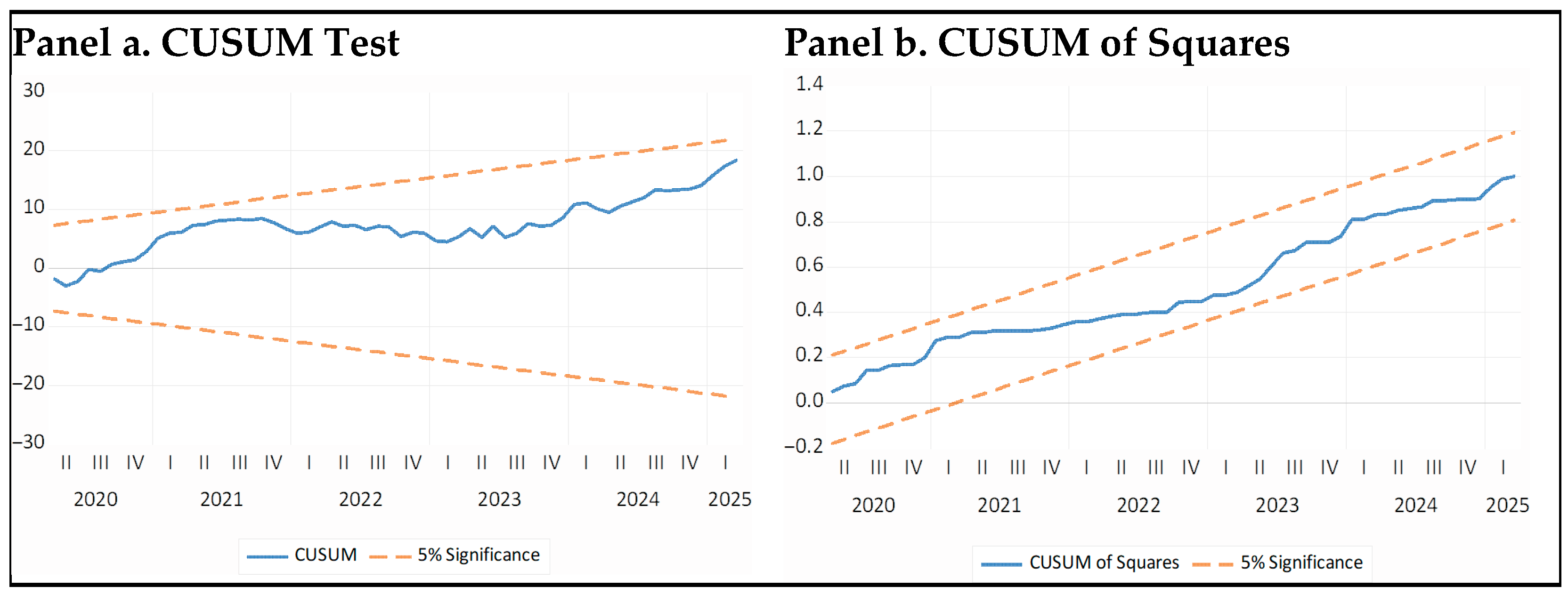
The error correction term (ECM = −0.33) is negative and highly significant, confirming the existence of a stable long-run equilibrium relationship. Diagnostic statistics further confirm that the model is well specified, free from serial correlation and heteroskedasticity, and that residuals are normally distributed. The stability of the estimated model was further examined through the CUSUM and CUSUM of squares tests. Both test statistics remain well within the 5% significant bounds across the entire sample period, as can be seen in Appendix A.

4.2. Asymmetric Model

The optimal lag length was determined using the AIC, and the selected specification for the asymmetric trade balance model was identified as NARDL (10, 4, 0, 4). The calculated F-statistic (8.09) exceeds the upper critical bound at the 1% significance level, leading to the rejection of the null hypothesis of no cointegration. This confirms the existence of a long-run relationship among the variables in the NARDL model. Furthermore, to examine whether the relationship between real exchange rate movements and the trade balance is symmetric or asymmetric, the Wald symmetry test was conducted.

Table 4. The result of short- and long-run asymmetries.

Variable	F-Statistic	p-Value
Ho: $\sum {\mathsf{\gamma }}_{4\mathrm{j}}=\sum {\mathsf{\gamma }}_{5\mathrm{j}}$ (Short-run) and ${\mathsf{\theta }}_4={\mathsf{\theta }}_5$ (Long-run)
LREX (Long-run)	5.6804 **	0.0189
LREX (Short-run)	9.7667 ***	0.0023
LREX (Joint)	6.3149 ***	0.0025

*** means statistical significance at the 1% level and ** statistical significance at the 5% level.

reports the corresponding results. The null hypothesis of coefficient symmetry is rejected at the 5% significance level in both the short run (F = 9.77, p = 0.0023) and the long run (F = 5.68, p = 0.0189). The joint Wald statistic (F = 6.31, p = 0.0025) also rejects the null hypothesis, confirming the presence of asymmetric adjustment

The observed asymmetry in Table 4 reflects well-documented economic mechanisms including sunk market entry costs, pricing-to-market behavior, and rigidity in import demand, which are discussed in detail in Section 5. In brief, Turkish exporters that have already incurred the fixed costs of accessing the German market are unlikely to retreat when the lira appreciates, while import demand for German capital goods and intermediates remains relatively price-inelastic, dampening the symmetric adjustment that standard models would predict.

Having established the presence of both short-run and long-run asymmetries,

Table 5. Estimated long and short run results in asymmetric model (10, 4, 0, 4, 4).

	Coefficient	Std. Error	t-Statistic	p-Value
Dependent Variable: LTB
Panel A: Long-run Coefficients
LYTR	−0.92 ***	0.34	−2.70	0.00
LYGR	1.76 ***	0.45	3.84	0.00
LREX-POS	0.28 *	0.15	1.80	0.07
LREX-NEG	−0.04	0.21	−0.18	0.85
Panel B: Short-run Coefficients
$∆$LTB (−1)	−0.30 ***	0.08	−3.51	0.00
$∆$LTB (−2)	−0.14	0.09	−1.61	0.11
$∆$LTB (−3)	0.03	0.09	0.33	0.73
$∆$LTB (−4)	0.06	0.08	0.72	0.46
∆LTB (−5)	0.06	0.08	0.73	0.46
∆LTB (−6)	0.15 *	0.08	1.75	0.08
∆LTB (−7)	0.27 ***	0.08	3.16	0.00
∆LTB (−8)	0.32 ***	0.08	3.82	0.00
∆LTB (−9)	0.28 ***	0.07	3.81	0.00
$∆$YTR	0.09	0.14	0.65	0.51
$∆$YTR (−1)	−0.20	0.14	−1.40	0.16
$∆$YTR (−2)	−0.04	0.14	−0.30	0.76
$∆$YTR (−3)	−0.51 ***	0.14	−3.57	0.00
$∆$REX-POS	0.89 ***	0.25	3.44	0.00
$∆$REX_POS (−1)	−0.40	0.27	−1.46	0.14
$∆$REX_POS (−2)	0.34	0.30	1.11	0.26
$∆$REX_POS (−3)	0.32	0.29	1.09	0.27
$∆$REX_NEG	−0.68 **	0.32	−2.10	0.03
∆REX_NEG (−1)	0.09	0.32	0.30	0.76
∆REX_NEG (−2)	−0.45	0.29	−1.54	0.12
∆REX_NEG (−3)	−0.58 **	0.29	−1.99	0.04
DUM2020	0.06 ***	0.01	3.70	0.00
C	0.015	0.01	1.25	0.21
ECM	−0.47 ***	0.07	−6.47	0.00
Panel C: Diagnostic Test Results
		Test Statistics	p-Value
Serial Correlation (Breusch–Godfrey)		F = 0.76	0.67
Heteroskedasticity (Breusch–Pagan–Godfrey)		F = 0.82	0.70
Model Specification (Ramsey RESET)		F = 1.46	0.23
Normality of Residuals (Jarque–Bera)		JB = 0.17	0.92
Panel D: Bounds Test for Cointegration
F-statistic (k = 4)		F = 8.09	greater than the 1% upper critical value

*** denotes significance at 1%, ** denotes significance at 5% and * denotes significance at 10%. k is the number of regressors. Note: Critical values are drawn from Narayan (2005).

reports the corresponding NARDL estimates for the asymmetric model, highlighting the separate effects of real depreciations and appreciations on the manufacturing trade balance.

The long-run coefficients presented in Panel A indicate that the income level of Türkiye (LYTR) has a negative and statistically significant coefficient (−0.92, p < 0.01), suggesting that an increase in domestic income leads to a deterioration in the trade balance, likely due to a rise in import demand. Conversely, the income level of Germany (LYGR) has a positive and highly significant coefficient (1.76, p < 0.01), implying that Germany’s income growth stimulates Türkiye’s exports, thereby improving the trade balance.

Regarding the real exchange rate, the positive partial sum variable (REX_POS), representing real depreciation of the Turkish lira, has a positive coefficient (0.28) that is significant. This indicates that a depreciation of the real exchange rate improves the trade balance in the long run. On the other hand, the negative partial sum variable (REX_NEG), corresponding to real appreciation, is statistically insignificant, implying that an appreciation of the lira does not have a meaningful long-run effect on trade balance dynamics.

The short-run dynamics are reported in Panel B. The first lag of the trade balance ∆LTB (−1) is negative and highly significant. The short-run coefficients for Türkiye’s income are negative at lag 3. For the real exchange rate components, the positive partial sum capturing depreciation, ∆REX_POS, is positive and highly significant, showing that lira depreciation leads to an improvement in the trade balance in the short run. In contrast, the negative partial sum, ∆REX_NEG, reflecting appreciation, is negative and significant. A positive and significant coefficient on the COVID-19 dummy implies that, conditional on other regressors, the bilateral manufacturing trade balance with Germany improved during the pandemic period, pointing to COVID-19-related shifts in trade patterns.

The observed asymmetry between the depreciation and appreciation effects documented in Table 4 reflects several well-established economic mechanisms. Turkish exporters that have already incurred the sunk costs of accessing the German market—through certifications, distribution networks, and supplier relationships—are unlikely to exit when the lira appreciates, dampening the symmetric trade balance deterioration that standard models would predict. At the same time, pricing-to-market behavior allows exporters to absorb appreciation by compressing profit margins rather than raising euro-denominated prices, while import demand for German capital goods and intermediate inputs remains relatively price-inelastic given its ties to production schedules. These mechanisms are discussed in greater detail in Section 5.

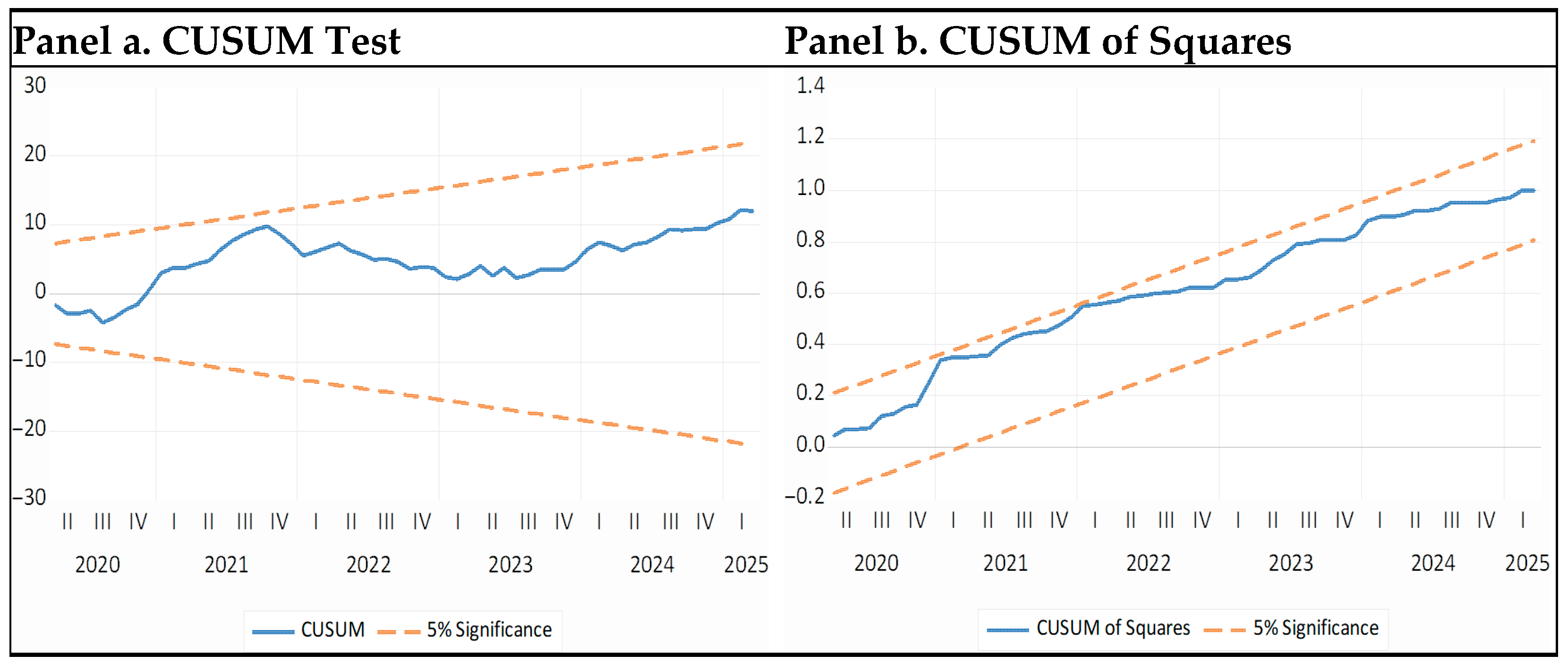
The error correction term (ECM) is negative (−0.47) and significant at the 1% level, indicating that approximately 47% of short-run disequilibria are corrected each month. The diagnostic test results reported in Panel C confirm the robustness of the model. Furthermore, the stability of the model parameters was assessed using the CUSUM and CUSUM of squares tests. As can be seen in Appendix A, both statistics remain within the 5% significance bounds throughout the sample period, confirming the absence of structural instability or parameter shifts.

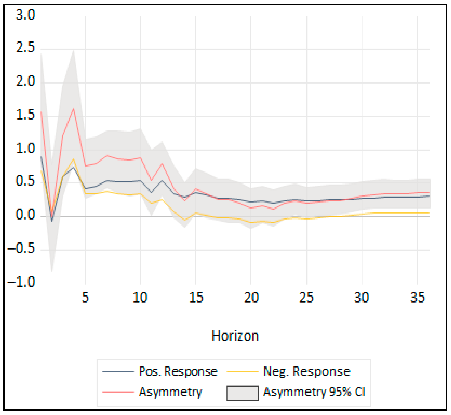
The dynamic multiplier results in Figure 1 show how the bilateral manufacturing trade balance adjusts to real exchange rate shocks over time. In the case of depreciation, the trade balance first deviates noticeably from its baseline and then improves gradually, settling at a higher level in the medium term. An appreciation, by contrast, leads to only small and short-lived changes, with the trade balance staying close to its initial path at most horizons. Overall, the trade balance reacts much more strongly to depreciations than to appreciations, which is consistent with the Wald test evidence of significant long-run and short-run asymmetry in the NARDL model.

4.3. Robustness: REER-Based Specification

The robustness of the baseline results is assessed by re-estimating the NARDL model using an alternative real effective exchange rate measure. Specifically, the bilateral real exchange rate is replaced with a real effective exchange rate index that captures Türkiye’s overall price competitiveness vis-à-vis its main trading partners.7 The alternative specification yields long-run and short-run coefficients that are broadly consistent with the baseline estimates: real depreciations continue to be associated with an improvement in the manufacturing trade balance, whereas appreciations exert weaker and often insignificant effects (

Table 6. Symmetric and asymmetric NARDL estimates (REER-based robustness model).

	Symmetric Model (10, 4, 0, 5)		Asymmetric Model (10, 1, 0, 0)
	Coefficient	p-Value	Coefficient	p-Value
Dependent Variable: LTB
Panel A: Long-run Coefficients
LYTR	0.06	0.85	−1.22 ***	0.00
LYGR	0.82 **	0.05	1.75 ***	0.00
LREER	0.31	0.21
LREER-POS			0.50 ***	0.00
LREER-NEG			0.09	0.64
Panel B: Short-run Coefficients
$∆$LTB (−1)	−0.35 ***	0.00	−0.27 ***	0.00
$∆$LTB (−2)	−0.15 *	0.09	−0.046	0.61
$∆$LTB (−3)	0.15 *	0.10	0.09	0.30
$∆$ LTB (−4)	0.14	0.11	0.12	0.15
∆LTB (−5)	0.13	0.13	0.16 *	0.07
∆LTB (−6)	0.22 ***	0.01	0.29 ***	0.00
∆LTB (−7)	0.28 ***	0.00	0.30 ***	0.00
∆LTB (−8)	0.31 ***	0.00	0.36 ***	0.00
∆LTB (−9)	0.24 ***	0.00	0.28 ***	0.00
$∆$LYTR	0.45 ***	0.00	0.18	0.25
$∆$YTR (−1)	−0.28 **	0.05
$∆$LYTR (−2)	−0.22	0.11
$∆$LYTR (−3)	−0.58 ***	0.00
$∆$LREX	0.34 *	0.06
$∆$LREX (−1)	−0.22	0.22
$∆$LREX (−2)	0.38 **	0.05
$∆$LREX (−3)	−0.25	0.16
$∆$LREX (−4)	0.60 ***	0.00
DUM2020	0.03	0.11	0.06 ***	0.00
C	0.57	0.00	0.63 ***	0.00
ECM	−0.32 ***	0.00	−0.45 ***	0.00
	F-Test		F-Test
Bounds test	5.89 ***		6.82 ***
Wald Symmetry Test (Long-Run)			7.23 ***	0.01

*** denotes significance at 1%, ** denotes significance at 5% and * denotes significance at 10%.

). The Wald statistics in the REER-based model likewise reject the null of symmetry in the long run, indicating that the evidence of asymmetric exchange rate effects on the bilateral manufacturing trade balance is not sensitive to the choice of the exchange rate indicator.

Furthermore, a set of standard diagnostic checks confirms that both the symmetric and asymmetric specifications are statistically adequate. The models do not exhibit major problems related to serial correlation, heteroskedasticity, misspecification, or parameter instability, and the residual behavior is consistent with the assumptions underlying the ARDL/NARDL framework.

5. Discussion

Neither the symmetric nor the asymmetric models confirm the validity of the J-curve effect in the manufacturing sector trade balance between Türkiye and Germany. This result is consistent with the findings of Rose (1990), Bahmani-Oskooee and Malixi (1992), Brada et al. (1997), Akbostanci (2004), and Bahmani-Oskooee and Kutan (2009). However, similarly to Karamelikli (2016) and Bahmani-Oskooee and Karamelikli (2020)—both of which also examined the Türkiye–Germany trade balance—the asymmetric model produces more significant results.

In the symmetric specification, the real exchange rate does not exert a significant long-run effect on the manufacturing trade balance, suggesting that depreciations and appreciations are treated as having the same impact. By contrast, the asymmetric NARDL estimates reveal that real depreciations of the Turkish lira are associated with an improvement in the trade balance, whereas appreciations have weak or insignificant effects. Moreover, moving from the symmetric to the asymmetric specification also improves the behavior of the control variables: the coefficients on domestic and foreign income and on the COVID-19 dummy become more precisely estimated, display the expected signs, and are generally statistically significant. In addition, the robustness analysis based on the alternative real effective exchange rate measure shows a similar improvement when moving from the symmetric to the asymmetric specification, reinforcing the conclusion that allowing for asymmetry yields a more informative and empirically plausible characterization of the exchange rate–trade balance relationship. The asymmetric NARDL estimates reveal that real depreciations of the Turkish lira are associated with an improvement in the trade balance, whereas appreciations have weak or insignificant effects. This pattern is consistent with the view that sunk entry costs (A. C. Arize et al., 2017), pricing-to-market behavior (Bhat & Bhat, 2021) and expectations of future policy interventions make exporters more reluctant to adjust quantities or exit foreign markets when the lira appreciates than when it depreciates (Bhat & Bhat, 2021; Bahmani-Oskooee & Fariditavana, 2015, 2016).

Moreover, the positive, significant and robust coefficient on the COVID-19 dummy indicates that, conditional on other regressors, the bilateral manufacturing trade balance with Germany improved during the pandemic period. In the symmetric specification, this net effect is not statistically detectable, but once asymmetric responses to depreciations and appreciations are allowed for, the positive and significant COVID-19 coefficient indicates that the pandemic period was associated with an improvement in Türkiye’s bilateral manufacturing trade balance with Germany. The insignificance of this coefficient in the symmetric specification is consistent with economic expectations: the pandemic disrupted exports and imports simultaneously, generating partially offsetting effects on the bilateral trade balance that cancel out when depreciation and appreciation are constrained to a single coefficient. Once asymmetric responses are allowed for, the nonlinear framework is able to isolate the net positive impact—suggesting that the pandemic-era depreciation of the Turkish lira interacted with the asymmetric exchange rate pass-through to amplify the improvement in the trade balance beyond what non-price factors alone would predict. This finding can be interpreted as evidence that COVID-19 induced non-price shifts in trade patterns. Supply chain disruptions and demand contractions in Germany and other advanced economies appear to have reduced their exports more strongly than their imports, while Türkiye’s manufacturing exports recovered relatively quickly, thereby moving the bilateral balance in Türkiye’s favor despite the overall collapse in global trade. In addition, sectoral evidence suggests that the pandemic affected industries asymmetrically, with certain categories of manufactured goods—such as intermediate and essential products—proving more resilient or even experiencing heightened demand, which may have reinforced the relative advantage of Türkiye’s manufacturing export basket vis-à-vis Germany.

These results suggest that relying solely on a standard symmetric framework may lead to misleading policy conclusions, because it implicitly assumes that depreciations and appreciations of the Turkish lira have identical effects on the manufacturing trade balance. Once asymmetric responses are taken into account, it becomes clear that real depreciations play a much more prominent role than appreciations, implying that policymakers need to explicitly distinguish between the two when designing exchange-rate-based trade policies. Moreover, the findings highlight the importance of accounting for cross-country and sectoral heterogeneity; a one-size-fits-all view of the exchange-rate–trade nexus is likely to obscure relevant differences across trading partners and industries and may therefore result in inappropriate policy prescriptions, especially when policies are not tailored to the specific partner country under consideration. In practice, this means that policy recommendations should be formulated with explicit reference to the particular bilateral relationship—such as Türkiye’s manufacturing trade with Germany—rather than being generalized across all partners. Finally, the lack of evidence for a conventional J-curve pattern indicates that exchange rate movements do not generate a systematic short-run deterioration followed by an automatic long-run improvement in the trade balance, reinforcing the need for a more nuanced, asymmetric and disaggregated approach to policy design.

While these results are informative, they should be interpreted in light of several limitations. The analysis focuses exclusively on bilateral manufacturing trade between Türkiye and Germany, so the documented asymmetric J-curve patterns may not directly generalize to other partners or sectors, nor do they explicitly account for Türkiye’s position in global value chains. Future research could therefore extend the asymmetric framework to other major trading partners, additional sectors and more disaggregated product-level and value-chain-related data to assess how robust these findings are across different dimensions.

6. Conclusions and Policy Implications

This paper has investigated whether movements in the real exchange rate generate an asymmetric J-curve in the manufacturing trade between Türkiye and Germany, that is, whether real depreciations and appreciations of the Turkish lira have different short-run and long-run effects on the bilateral manufacturing trade balance. The analysis, based on monthly data for 2013M01–2025M07 and on symmetric ARDL and asymmetric NARDL specifications, finds no evidence of a conventional J-curve pattern in the manufacturing trade balance. Instead, while the symmetric model suggests a weak and often insignificant role for the real exchange rate, the asymmetric specification uncovers a clear difference between the effects of depreciations and appreciations: real depreciations are associated with an improvement in the manufacturing trade balance in both the short and long run, whereas appreciations exert only weak or statistically insignificant effects. Because the empirical exercise is confined to manufacturing trade between Türkiye and Germany, these findings should be interpreted as pertaining to this specific bilateral and sectoral setting rather than to Türkiye’s external trade in general.

These results have important implications for exchange-rate-based trade policy. First, they show that a purely symmetric perspective on exchange rate movements can be misleading, because it implicitly treats depreciations and appreciations of the lira as having identical effects on trade. Policy assessments that rely only on symmetric models risk underestimating the potential gains from real depreciations or overstating the costs of appreciations, and may therefore lead to incorrect conclusions about the effectiveness of exchange rate adjustments as an instrument for correcting external imbalances. Second, the evidence emphasizes the relevance of cross-country and sectoral heterogeneity. The response of manufacturing trade between Türkiye and Germany cannot simply be extrapolated to other partners or industries; a one-size-fits-all view of the exchange-rate–trade nexus is likely to obscure important differences and produce misguided policy recommendations. Moreover, the COVID-19 dummy suggests that pandemic-related shocks can alter trade patterns through non-price channels, highlighting the need for policies that strengthen supply chain resilience and support those manufacturing segments—especially intermediate and essential goods—where Türkiye can act as a reliable supplier to partners such as Germany during global disruptions.

From a practical policy standpoint, the findings suggest that exchange rate strategies should explicitly incorporate asymmetric responses into their design. Real depreciations can support the manufacturing trade balance with Germany, but their impact appears to work through gradual competitiveness gains rather than through a standard J-curve mechanism that guarantees an initial deterioration followed by an automatic long-run improvement. Policymakers should therefore avoid relying on short-lived nominal changes or on the expectation of a mechanical J-curve, and instead focus on maintaining a consistent macroeconomic environment in which real depreciations—when they occur—are complemented by structural and industrial policies that enhance export capacity in manufacturing. At the same time, given that the analysis is restricted to a single trading partner and sector, exchange rate policy should be formulated with an awareness that other bilateral relationships and sectors may exhibit different degrees and patterns of asymmetry.

Finally, the study points to several avenues for further research. Future work could extend the asymmetric framework to other major trading partners and sectors, and employ more disaggregated product-level and value-chain-related data to clarify the channels through which exchange rate movements affect trade flows.