Inflation Shocks and Equity Vulnerability: Regime, Sign, and Cross-Country Asymmetries in the G7

Abstract

This paper investigates the nonlinear and state-dependent relationship between inflation surprises and real equity returns across G7 economies. Using monthly data from January 1998 to May 2025, we employ nonlinear local projection models to estimate the dynamic responses of the equity market to domestic inflation shocks. While linear estimates reveal modest but persistent average losses, once regime dependence and sign asymmetry are jointly considered, three critical findings emerge. First, equity responses are strongly regime-dependent: inflation shocks occurring in high-inflation environments produce losses two to four times larger than those in low-inflation regimes. Second, the direction of the shock matters: positive inflation surprises are associated with deeper and longer-lasting equity declines than the gains generated by negative surprises. Third, these effects exhibit pronounced cross-country heterogeneity, with distinct vulnerability profiles that remain invisible in linear or pooled models. To systematically assess these differences, we develop a Sensitivity–Volatility–Vulnerability (SVV) assessment that synthesizes regime-dependent and sign-asymmetric responses into market vulnerability profiles. Our results underscore that inflation risk in equity markets is not only nonlinear and regime-dependent but also fundamentally country-specific, implying that conventional linear models materially understate downside equity exposure. These findings carry important implications for monetary policy, financial regulation, and international portfolio diversification.

1. Introduction

This paper focuses on how real equity returns respond to inflation surprises across horizons and regimes in G7 economies. After decades of low, stable inflation, the post-2021 surge in consumer prices revived concerns about inflation risk in equity valuations. Markets reacted unevenly across countries and over time, raising a fundamental question for asset pricing and risk management: Do equity markets respond symmetrically to inflation news, or does the effect depend on the inflation environment and the direction of the surprise?

Standard asset-pricing frameworks predict that equity prices will respond negatively to unexpected inflation, driven by higher discount rates and compressed real cash flows. A large body of the empirical literature confirms this relationship on average, particularly for advanced economies. Yet, the evidence is far from uniform. Estimated effects vary widely across periods, countries, and inflation environments, and in some cases even change sign. These inconsistencies suggest that the inflation–equity nexus is not well characterized by a stable linear relationship. The transmission mechanism is not a static, linear channel but rather a dynamic process that depends on unobserved state variables.

Two dimensions of nonlinearity are especially relevant to financial markets, and, critically, they may interact. First, the inflation regime matters. When inflation is already elevated, investors may price in a more persistent and aggressive path of monetary tightening, amplifying valuation losses. When inflation is low and stable, the same surprise may trigger weaker repricing. Second, the sign of the inflation shock matters. Upside inflation surprises may be penalized more severely than downside surprises are rewarded, implying an asymmetric or convex equity loss function.

However, existing empirical work typically examines these dimensions in isolation. Studies of regime dependence focus on high-versus-low-inflation environments (Boyd et al., 2005; Bekaert & Engstrom, 2010; Chen et al., 2023; Chiang, 2025; Muguto & Muzindutsi, 2022; Caporale et al., 2022), whereas work on sign asymmetry emphasizes positive-versus-negative inflation news (Rigobon & Sack, 2004; Erdoğan & Tiryaki, 2018). While these nonlinear approaches are well established, no study has systematically and jointly estimated how the equity market’s response to inflation news depends on both the sign of the surprise and the prevailing inflation regime across a wide range of advanced economies. This gap is substantive because the two nonlinearities likely interact: for instance, the penalty for positive inflation surprises may be amplified when inflation is already elevated, or the effect of negative surprises may depend on whether the economy is in a high- or low-inflation state. Our paper fills this gap by integrating and extending existing nonlinear approaches by introducing a unified framework that simultaneously accounts for regime dependence and sign asymmetry, allowing us to estimate what we term the ‘double asymmetry’ in the inflation–equity nexus.

To test these propositions, we use two key methodological advances and a new empirical approach. First, we analyze the responses of G7 equity markets using the local projections (LPs) method (Jordà, 2005, 2023). Second, we extend our framework to account for nonlinearities, enabling us to differentiate the effects of positive and negative inflation surprises, as well as those in high- and low-inflation regimes. This method enables us to measure horizon-specific effects while accounting for asymmetry and variations in responses in our research.

Our results confirm a strong and statistically significant double asymmetry, but with an important caveat. We find that, for most G7 nations, including the United States, Germany, and the United Kingdom, high-inflation regimes act as powerful amplifiers, and positive surprises lead to deep and lasting declines in equity, while negative surprises provide little relief. However, this pattern is sharply broken by Italy, where low inflation and disinflationary surprises cause the most severe market penalties. France appears remarkably shielded, likely due to its economic structure. These exceptions are not merely outliers; they may suggest that country-specific institutions and vulnerabilities fundamentally alter the inflation–equity relationship.

In this paper, we first provide updated linear estimates for all G7 markets, confirming the negative impact—consistent with Stock and Watson (2009) but contrasting with the null results in Geske and Roll (1983). Second, we show that the same surprise causes equity losses to be two to four times higher when headline inflation exceeds its historical median, consistent with the findings proposed by Nakamura and Steinsson (2018). Third, we implement a joint Regime–Sign asymmetry framework that estimates responses across four distinct states (low-positive, low-negative, high-positive, high-negative). This allows us to test whether the amplification effect of high inflation depends on the direction of the surprise, and whether the penalty for positive surprises varies across inflation regimes—questions that cannot be answered by studying regime dependence or sign asymmetry separately.

Fourth, the paper offers a comprehensive cross-country comparison of the G7 nations—Canada, France, Germany, Italy, Japan, the United Kingdom, and the United States—revealing systematic differences in shock transmission that are often obscured by single-country studies or pooled regressions. Fifth, the analysis incorporates medium- and long-term dynamics through a horizon-specific framework, moving beyond typical short-term event windows to assess whether market reactions persist, reverse, or amplify over horizons up to one year. This temporal mapping helps determine whether inflation shocks lead to temporary disruptions or have lasting effects on valuations, addressing a gap in research that mainly focuses on immediate impacts. In this study, we use the local projections (LPs) approach to generate robust estimates tailored to different time horizons. This method accounts for differences across countries, making it more reliable than traditional time-series models.

Finally, we develop a composite Sensitivity–Volatility–Vulnerability (SVV) assessment that goes beyond impulse response magnitudes to evaluate the stability of responses across inflation regimes. This framework shows that the effects of inflation shocks depend not only on their sign and regime but also on the structural capacity of markets to absorb or amplify volatility. By combining the magnitude of regime effects, the rise in uncertainty, and directional asymmetry in shock transmission, the SVV measure identifies different vulnerability profiles across the G7.

This new perspective changes how we understand the connection between inflation and stock markets. It focuses on financial resilience rather than just how prices react. Importantly, our interpretation remains disciplined. Our empirical design identifies conditional responses rather than causal mechanisms. We therefore treat these channels as interpretive rather than directly tested.

From a finance and economic perspective, the findings imply that inflation risk is neither uniform nor linear. Equity vulnerability depends on when inflation shocks occur and on the direction of the surprise. Simple diversification across advanced economies does not eliminate inflation risk, and models based on average sensitivities materially understate downside exposure.

This paper is organized as follows. Section 2 reviews the literature on inflation and equity markets. Section 3 presents the empirical framework and preliminary results. Section 4 analyzes regime- and sign-dependent responses to inflation shocks. Section 5 explores joint regime–sign asymmetries. Section 6 interprets cross-country heterogeneity. Section 7 develops the Sensitivity–Volatility–Vulnerability (SVV) assessment. Section 8 summarizes the findings and discusses policy implications. Finally, Section 9 concludes with recommendations for future research.

2. Literature Review

The relationship between inflation and equity returns has been a central yet elusive subject, and the literature has evolved from establishing basic correlations to acknowledging increasingly complex layers. The literature can be organized along three complementary dimensions: linear average-effect models, regime-dependent frameworks, and sign-asymmetry approaches. This section reviews each strand in turn and clarifies how the present framework integrates them.

We begin with the linear literature, which estimates the average response of equity returns to inflation shocks under the assumption of parameter constancy. Since Fisher (1930), conventional theory has held that nominal stock returns should keep pace with inflation, implying a positive long-run link between them (Levant et al., 2013). Under this view, equities serve as a natural hedge, preserving real value when prices rise. However, a substantial body of research found that higher inflation tends to coincide with lower stock returns (Groenewold et al., 1997; Kim, 2003; Chiang, 2023).

Nelson (1976) and Fama (1981) recorded a negative link between inflation and U.S. stock prices. They attribute these results to the decline of real activity and the tightening of the monetary policy. The studies have identified two major transmission channels that could explain these findings: the discount-rate channel and the cash flow channel. Through the discount-rate channel, a rise in inflation expectations prompts central banks to raise interest rates, thereby reducing the discounted value of future corporate earnings (Modigliani & Cohn, 1979; Campbell & Viceira, 2002). On the other hand, the cash flow channel stipulates that firms face some operational constraints. Nominal rigidities in many corporations often prevent them from fully passing higher costs to consumers, thereby compressing margins and weakening valuations (Fama, 1981; Geske & Roll, 1983).

As evidence of negative correlations persisted, researchers turned to more sophisticated methods. Berument and Jelassi (2002) attempted to model lags in inflation’s impact, but results remained inconclusive. Malliaropulos (2000) asserted that the negative linkages were exaggerated because the structural changes in the data were ignored. By addressing these statistical concerns, Engsted and Tanggaard (2002), Anari and Kolari (2001), and Boudoukh and Richardson (1993) confirmed a sustained positive relationship, supporting the view that equities hedge against inflation.

Ryan (2006) and Wong and Wu (2003) documented Fisher effects in Ireland, Asia, and the G7, while Solnik and Solnik (1997) and Toyoshima and Hamori (2011) reached similar conclusions.

This ambiguity in the findings suggests a fundamental limitation of the linear models presented so far. By imposing parameter constancy, they obscure the possibility that the inflation–equity nexus is not a static channel but may be a dynamic process dependent on unobserved state variables.

For that reason, other research has turned toward nonlinear explanations, and a second strand of the literature introduces regime dependence. The relationship is, in fact, state-dependent, and the macroeconomic environment powerfully modulates how equities process inflation news. These studies aimed to suggest that inflation’s influence on equity markets depends less on its presence than on its character and intensity. Ahmad (2010) used threshold models to show that the effect of inflation flips sign depending on its level—positive at moderate levels and negative at high levels. Boyd et al. (2005) showed that U.S. equities react positively to “bad” macroeconomic news (including lower inflation) only during recessions. Bekaert and Engstrom (2010) documented that the relationship holds during disinflation but breaks down when inflation expectations are high. Nakamura and Steinsson (2018) provided a theoretical mechanism, arguing that, when inflation expectations are unanchored, the same news can provoke a convex response in discount rates. Hess and Lee (1999) have also linked these dynamics to the source of inflation. Demand-driven inflation tends to correlate with higher returns, while inflation driven by a supply shortage depresses them. Hondroyiannis and Papapetrou (2006) and Muhammad et al. (2024) demonstrate that volatility and return dynamics shift with inflation states and policy responses. McMillan (2017) has demonstrated that mild inflation signals sustainable growth, whereas pronounced high inflation erodes investor confidence and expected returns. All these studies establish a crucial principle: the prevailing inflation regime acts as a powerful amplifier.

A third strand focuses on sign asymmetry, examining whether equity markets respond differently to positive versus negative inflation surprises. What matters here is the direction of the inflationary shock. Using a nonlinear autoregressive distributed lag framework, Alqaralleh (2020) concludes that positive and negative inflation shocks cause different and asymmetric responses in stock prices. Rigobon and Sack (2004), using heteroskedasticity-based identification, found that the S&P 500 responds asymmetrically to CPI releases, with upside surprises triggering larger reactions. These results align with theoretical models featuring downward nominal wage rigidity or constraints on monetary policy (Auclert et al., 2025), which predict that positive shocks amplify financial constraints more than negative shocks relieve them. It seems that investors punish rising inflation more severely than they reward falling inflation. Yet, sign-asymmetry studies are rare and have typically been confined to single-country settings, primarily the United States.

Other contextual factors also shape the outcomes across time and region. Bhanja and Dar (2019) found that the market ability to hedge inflation has shifted with structural reforms in India. In Pakistan, wavelet analysis by Tiwari et al. (2015) revealed time-varying connections between inflation and stock indices. Chinese evidence suggests a positive long-term relationship during stable inflation periods, which weakens or turns negative as inflation accelerates (Jacob & Raphael, 2025; Yan, 2025). Results from Ghana show similar instability over time (Michael, 2014).

All these findings emphasize that local market structure, institutional settings, and economic reforms all mediate the inflation–equity dynamic. The inflation’s impact is context-dependent. It varies across regimes and policy environments. What emerges is not a universal rule but a dynamic and state-sensitive understanding of how inflation and stock markets interact across different economic landscapes.

The literature thus documents both state dependence and sign asymmetry in equity responses to inflation news, but these insights have largely developed along separate empirical lines. The empirical framework used here extends this literature by integrating both dimensions within a unified framework, enabling a systematic cross-country analysis of conditional equity responses.

3. Methodological Framework and Preliminary Results

To evaluate the dynamic effects of inflation shocks on stock market returns, we use the local projections (LPs) approach developed by Jordà (2005) and Barnichon and Brownlees (2019) separately for each G7 country. LP is suitable for our research goals for many reasons. First, it allows us to estimate responses at different horizons without relying on the strong symmetry or linearity constraints typical of Vector Autoregression (VAR) models. Second, LP is robust to model misspecification and does not require inverting the entire dynamic system, thereby reducing sensitivity to incorrect choices of lag length or variable order—issues common in macro-financial datasets that include economies with diverse monetary policies. Third, LP incorporates nonlinear and state-dependent features. We can estimate the impulse responses for inflationary and disinflationary surprises separately. LP directly estimates responses at each time period, which helps reduce errors that can affect long-term results in VARs. This leads to more accurate estimates of medium- and long-term effects. Since we want to measure how markets react in the short, medium, and long term to inflation shocks, LP provides a flexible and clear framework that meets both the theoretical and practical needs of our study.

We compile a balanced monthly panel of real total-return equity indices and consumer price inflation for the G7 economies from January 1998 to May 2025. Equity returns are converted to real terms (Δr_t) by deflating nominal total-return indices with the headline CPI; both series are expressed in log differences so that a one-unit change approximates a percentage-point move. Descriptive statistics appear in

Table 1. Descriptive statistics.

Inflation
	Canada	France	Germany	Italy	Japan	UK	USA
Obs	329	329	329	329	329	329	329
Mean	2.17%	1.62%	1.87%	2.02%	0.45%	2.38%	2.53%
Std	1.36%	1.28%	1.68%	1.89%	1.34%	1.60%	1.70%
Min	−0.95%	−0.73%	−0.50%	−0.58%	−2.50%	0.20%	−1.96%
25%	1.27%	0.80%	1.06%	0.90%	−0.40%	1.50%	1.61%
50%	2.01%	1.49%	1.53%	1.87%	0.10%	2.00%	2.26%
75%	2.62%	2.08%	2.07%	2.60%	0.81%	2.70%	3.22%
Max	8.13%	6.28%	9.99%	11.84%	4.39%	8.82%	8.99%
ADF	−2.872	−2.919	−3.247	−3.117	−1.710	−2.801	−3.196
KPSS	0.340	0.258	0.567	0.142	1.103	0.556	0.278
PP	−3.402	−2.942	−2.883	−3.104	−2.412	−2.749	−3.023
RRT
	Canada	France	Germany	Italy	Japan	UK	USA
Obs	329	329	329	329	329	329	329
Mean	−1.66%	−1.19%	−1.16%	−1.68%	−0.02%	−2.14%	−1.89%
Std	4.54%	5.47%	6.20%	6.53%	5.51%	4.24%	4.21%
Min	−21.09%	−19.34%	−26.68%	−22.54%	−25.53%	−17.82%	−17.51%
25%	−3.88%	−4.46%	−4.73%	−5.40%	−3.25%	−4.74%	−4.22%
50%	−1.10%	−0.72%	−0.82%	−1.08%	0.22%	−1.70%	−1.71%
75%	1.21%	2.21%	2.69%	2.09%	3.68%	0.62%	0.91%
Max	11.12%	19.92%	20.48%	23.15%	15.94%	11.75%	11.18%
ADF	−8.124	−7.338	−8.649	−6.616	−15.728	−5.563	−5.632
KPSS	0.107	0.112	0.174	0.095	0.136	0.325	0.250
PP	−14.841	−16.289	−16.553	−17.451	−15.965	−17.059	−17.089
Inflation vs. Return correlation	−0.392	−0.320	−0.317	−0.327	−0.235	−0.404	−0.385

.

Inflation surprises $∆{\pi }_t$ are defined as the demeaned month-on-month log change in CPI. To make responses economically comparable, we scale the shock by each country’s unconditional standard deviation, ${\sigma }_{\pi ,c}$, so that the impulse response function (IRF) traces the effect of a one-standard-deviation price surprise: ${\epsilon }_t^{\pi ,c}={\displaystyle \frac{∆{\pi }_t^c-\overline{∆{\pi }^c}}{{\sigma }_{\pi ,c}}}$. This normalization preserves cross-country heterogeneity in inflation volatility while providing directly comparable elasticities of real returns to a typical domestic shock. Moreover, this approach isolates the unexpected component of inflation by removing the predictable historical average. We employ month-on-month changes rather than year-on-year rates for two principal reasons. First, monthly innovations capture high-frequency information that is less contaminated by base effects and lagged price dynamics, thereby aligning more closely with the timing of monetary policy updates and market repricing. Second, using monthly data preserves a large time-series dimension, which is essential for estimating nonlinear and state-dependent responses over horizons up to one year. While year-on-year inflation reflects past shocks and may obscure the immediate news content that may shape equity markets.

The choice of a statistical surprise rather than a survey- or announcement-based forecast error stems from considerations of data availability, frequency, and cross-country consistency. Although survey measures provide a direct gauge of expectations, they are not uniformly available at a monthly frequency across all G7 economies over our full sample (1998–2025). High-frequency event-study proxies, such as the difference between released CPI figures and market expectations, provide clean identification but require tick-level data and are difficult to implement consistently across multiple countries spanning several decades. Our demeaning procedure effectively extracts the unanticipated component of inflation by removing its historical mean, a method widely adopted in macro-finance studies that prioritize long-span, balanced panels. This measure correlates strongly with periods of marked inflation volatility and exhibits time-varying linkages with equity returns.

Thus, our inflation surprise proxy represents a pragmatic yet theoretically grounded compromise: it ensures a consistent, high-frequency measure across all G7 countries while preserving the sample length necessary to detect regime-dependent and asymmetric effects. By scaling shocks by their country-specific standard deviations, we facilitate cross-country comparison while retaining meaningful differences in inflation volatility—a feature that linear pooled models often obscure. At the same time, this measure does not constitute a fully exogenous structural shock. Accordingly, the estimated impulse responses should be interpreted as conditional dynamic responses to observed inflation innovations rather than as causal effects.

Dynamic causal effects are estimated with Jordà’s (2005) local projection (LP) approach, which regresses the future value of the outcome on the shock and its lags without imposing VAR restrictions. For each horizon $h\in \left\{\mathrm{0,1},\dots ,12\right\}$ we run, country by country,

$$∆r_{t+h}^c={\alpha }_h^c+{\beta }_h^c{\epsilon }_t^{\pi ,c}+{\sum }_{j=1}^n{\gamma }_{h,j}^c{\epsilon }_{t-j}^{\pi ,c}+{\sum }_{j=1}^n{\delta }_{h,j}^c{∆r}_{t-j}^c+u_{t+h}^c$$

(1)

• $∆r_{t+h}^c$ is the real log return on country c’s equity index.
• ${\epsilon }_t^{\pi ,c}$ is the σ-standardized CPI surprise.
• ${\beta }_h^c$ = impulse response of real equity returns at horizon h to the contemporaneous one standard deviation inflation shock.
• ${\gamma }_{h,j}^c$, ${\delta }_{h,j}^c$ = coefficients on n of the shock and the dependent variable, controlling for serial dependence.
• ${\alpha }_h^c$ = horizon-specific intercept absorbing the unconditional mean.
• $u_{t+h}^c$ = error term.

Four lags are chosen to parallel a quarterly VAR at a monthly frequency; results are insensitive to eight-lag or two-lag alternatives. For the cumulative effects, the total wealth impact up to horizon h is ${CIRF}_h^c={\sum }_{k=0}^h{\beta }_k^c$.

Because CPI data are released after the month-end, the surprise ${\epsilon }_t^{\pi ,c}$ is uncorrelated with contemporaneous equity-return innovations under the standard no-leakage assumption, satisfying $\mathbb{E}\left(u_{t+h}^c\right|{\epsilon }_t^{\pi ,c})=0$.

This framework allows us to trace horizon-by-horizon and cumulative equity market conditional responses to typical domestic inflation surprises without imposing VAR dynamics, yielding policy-relevant, cross-country-comparable elasticities.

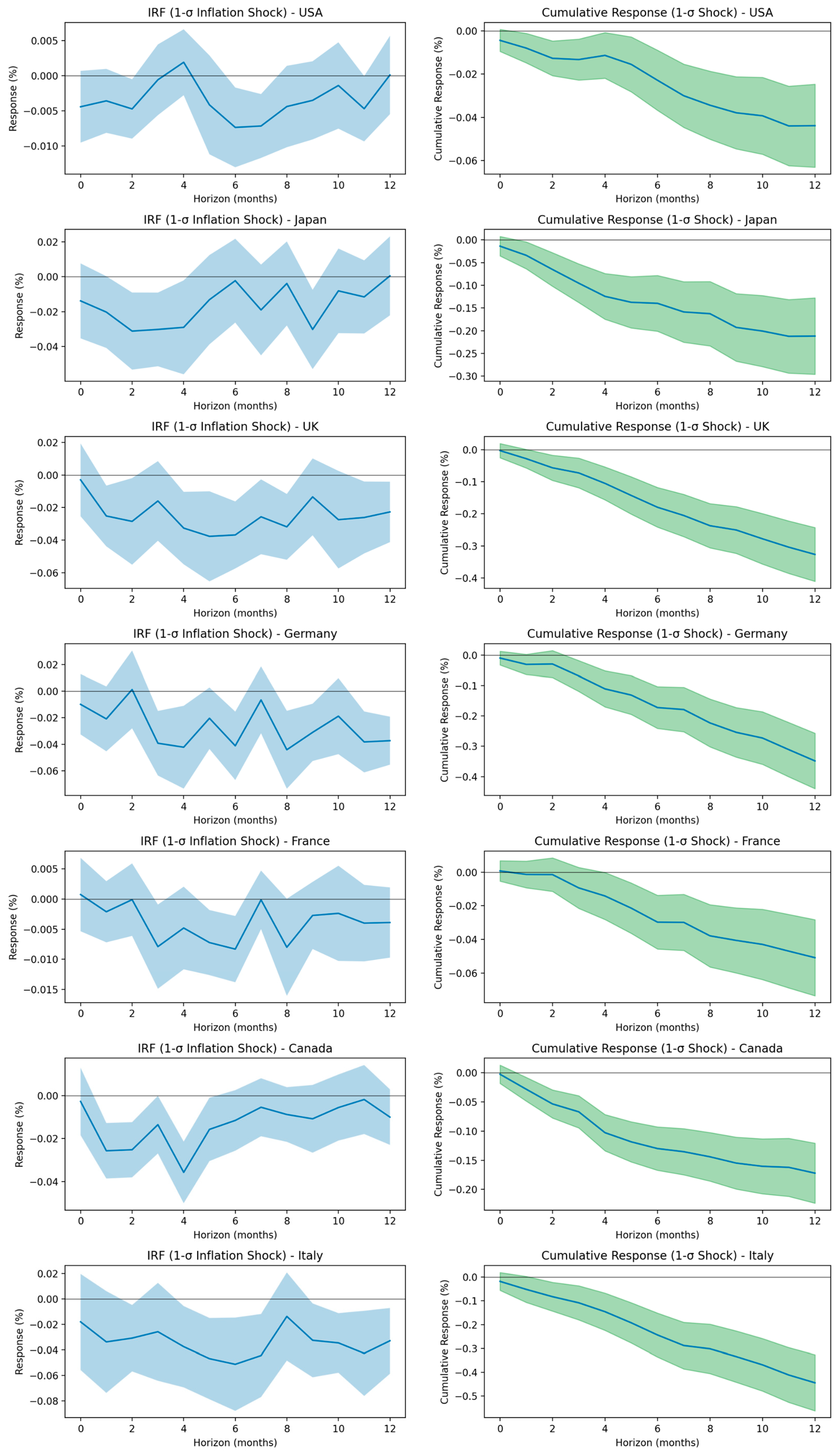
The empirical evidence reported in Figure 1 and

Table 2. IRFs results.

h	USA	Japan	UK	Germany	France	Canada	Italy
0	−0.0044 *	−0.0138	−0.0030	−0.0099	0.0008	−0.0026	−0.0179
1	−0.0036	−0.0202 **	−0.0252 ***	−0.0208 *	−0.0021	−0.0257 ***	−0.0337 *
2	−0.0047 **	−0.0311 ***	−0.0285 **	0.0013	−0.0001	−0.0252 ***	−0.0307 **
3	−0.0006	−0.0302 ***	−0.0159	−0.0392 ***	−0.0079 **	−0.0135 **	−0.0257
4	0.0019	−0.0290 **	−0.0326 ***	−0.0422 ***	−0.0048	−0.0357 ***	−0.0374 **
5	−0.0041	−0.0131	−0.0377 ***	−0.0204 *	−0.0072 ***	−0.0157 **	−0.0468 ***
6	−0.0074 **	−0.0022	−0.0368 ***	−0.0411 ***	−0.0083 ***	−0.0115	−0.0512 ***
7	−0.0072 ***	−0.0190	−0.0257 **	−0.0066	−0.0001	−0.0054	−0.0443 ***
8	−0.0044	−0.0038	−0.0318 ***	−0.0441 ***	−0.0080 *	−0.0087	−0.0137
9	−0.0035	−0.0302 ***	−0.0134	−0.0310 ***	−0.0027	−0.0108	−0.0324 **
10	−0.0014	−0.0081	−0.0274 *	−0.0188	−0.0024	−0.0055	−0.0345 ***
11	−0.0047 **	−0.0115	−0.0261 **	−0.0382 ***	−0.0040	−0.0018	−0.0426 **
12	0.0001	0.0005	−0.0227 **	−0.0373 ***	−0.0039	−0.0100	−0.0328 **

Significance: * for p < 0.1, ** for p < 0.05, and *** for p < 0.01.

shows that an unanticipated, one-standard-deviation increase in consumer price inflation reverberates through equity markets across the G7.

The impulse response analysis reveals significant and heterogeneous effects of inflation shocks on stock market returns across G7 countries. In fact, the immediate effect of inflation shocks (horizon 0) on G7 stock market returns is generally weak, negative, and statistically insignificant, except for the United States, where the response is small but significant at the 10% level (−0.0044), and for France, where the response is positive. This suggests that most G7 equity markets do not react sharply in the same month as the inflation shock, possibly due to information lags, market inertia, or delays in central bank signaling.

At the first-month horizon (h = 1), the effects become clearer and more significant. The UK experiences a significant decline in returns. This indicates a rapid and strong market repricing of inflation risks. Italy and Japan also show significant adverse effects. This reflects a higher sensitivity to inflation-driven changes. Germany and Canada follow with moderate negative and statistically significant responses, while France and the U.S. exhibit weak or insignificant reactions.

As shown in

Table 3. Time-horizon effects.

Country	Short-Term (h = 0–1)	Medium-Term (h = 2–6)	Long-Term (h = 7–12)
USA	Weak, marginally significant	Small, mixed	Minor, irregular
Japan	Significant early drop	Strong, peaks then fade	Weak to insignificant
UK	Sharp decline begins	Strong and persistent	Still significant
Germany	Modest initial drop	Large, persistent fall	Remains significant
France	Insignificant response	Mild, some significance	Mostly weak or nonsignificant
Canada	Strong at h = 1	Moderate, significant	Effects fade, mostly insignificant
Italy	Large negative impact	Strongest drop	Still significant

, three key patterns emerge. The UK, Germany, and Italy exhibit the most pronounced and persistent adverse effects, particularly in the medium- and long-term, indicating a deep sensitivity to inflation. Japan and Canada respond sharply in the short to medium term, but their effects dissipate over time. France and the USA show weaker and less consistent reactions, indicating relatively better absorption or delayed pricing of inflation shocks.

Panel B of Figure 1 converts the flow IRFs into stock measures by cumulating the coefficients. The trajectories confirm that inflation shocks deplete equity wealth across all markets. The results in

Table 4. Cumulative responses.

h	USA	Japan	UK	Germany	France	Canada	Italy
0	−0.0044 *	−0.0138	−0.0030	−0.0099	0.0008	−0.0026	−0.0179
1	−0.0080 **	−0.0340 **	−0.0281 *	−0.0307 *	−0.0013	−0.0283 ***	−0.0517 *
2	−0.0127 ***	−0.0652 ***	−0.0566 ***	−0.0294	−0.0014	−0.0535 ***	−0.0824 ***
3	−0.0133 ***	−0.0954 ***	−0.0726 ***	−0.0686 ***	−0.0093	−0.0670 ***	−0.1081 ***
4	−0.0114 **	−0.1244 ***	−0.1052 ***	−0.1108 ***	−0.0141 **	−0.1027 ***	−0.1455 ***
5	−0.0155 **	−0.1375 ***	−0.1428 ***	−0.1312 ***	−0.0214 ***	−0.1184 ***	−0.1923 ***
6	−0.0229 ***	−0.1397 ***	−0.1796 ***	−0.1723 ***	−0.0297 ***	−0.1300 ***	−0.2435 ***
7	−0.0300 ***	−0.1587 ***	−0.2053 ***	−0.1789 ***	−0.0298 ***	−0.1353 ***	−0.2878 ***
8	−0.0344 ***	−0.1626 ***	−0.2371 ***	−0.2230 ***	−0.0378 ***	−0.1441 ***	−0.3015 ***
9	−0.0379 ***	−0.1928 ***	−0.2506 ***	−0.2540 ***	−0.0405 ***	−0.1548 ***	−0.3339 ***
10	−0.0393 ***	−0.2008 ***	−0.2780 ***	−0.2728 ***	−0.0429 ***	−0.1603 ***	−0.3684 ***
11	−0.0440 ***	−0.2124 ***	−0.3041 ***	−0.3110 ***	−0.0469 ***	−0.1621 ***	−0.4110 ***
12	−0.0439 ***	−0.2118 ***	−0.3267 ***	−0.3483 ***	−0.0508 ***	−0.1721 ***	−0.4438 ***

Significance: * for p < 0.1, ** for p < 0.05, and *** for p < 0.01.

indicate that negative impacts intensify over time across all G7 economies.

These results highlight a pronounced asymmetry in how inflation shocks compound over time, with structurally more vulnerable markets—such as Italy, the UK, and Germany—experiencing the steepest cumulative declines. Furthermore, these magnitudes underscore that what begins as a seemingly small monthly effect can translate into a material erosion of purchasing-power-adjusted equity value. This suggests that market structure, inflation expectations, and monetary policy responsiveness play critical roles in determining the extent to which inflation shocks erode equity valuations over extended horizons.

In detail, several key points emerge from the analysis. First, there is a clear negative link between equity returns and inflation in advanced economies. Second, the impact of inflation varies across countries. Third, negative effects accumulate over time across all markets. Even countries that seem resilient experience significant losses in the long run. Fourth, in all G7 countries, long-term responses to inflation are negative and significant, suggesting a trend toward broader declines in equity markets when inflation shocks last. These patterns indicate that even short-lived inflation surprises can lead to significant and lasting losses in equity markets, with structural factors shaping the depth and persistence of the impact.

However, while the baseline linear IRFs capture the unconditional, average response of equity returns to inflation shocks, they implicitly assume that this relationship remains invariant across different economic conditions. This is a substantial restriction. Both theory and empirical evidence suggest that the equity–inflation linkage may vary with the prevailing inflation regime and the direction of the shock (Erdoğan & Tiryaki, 2018; Liu & Serletis, 2022; Chen et al., 2023; Chiang, 2025; Muguto & Muzindutsi, 2022; Caporale et al., 2022). For instance, when inflation is already high, markets may price in a greater likelihood of aggressive policy tightening, amplifying the adverse effect on equity valuations. On the opposite side, in low-inflation environments or when inflation is falling, the same shock magnitude may have a muted or even offsetting impact due to lower discount rate pressures or improved real income expectations.

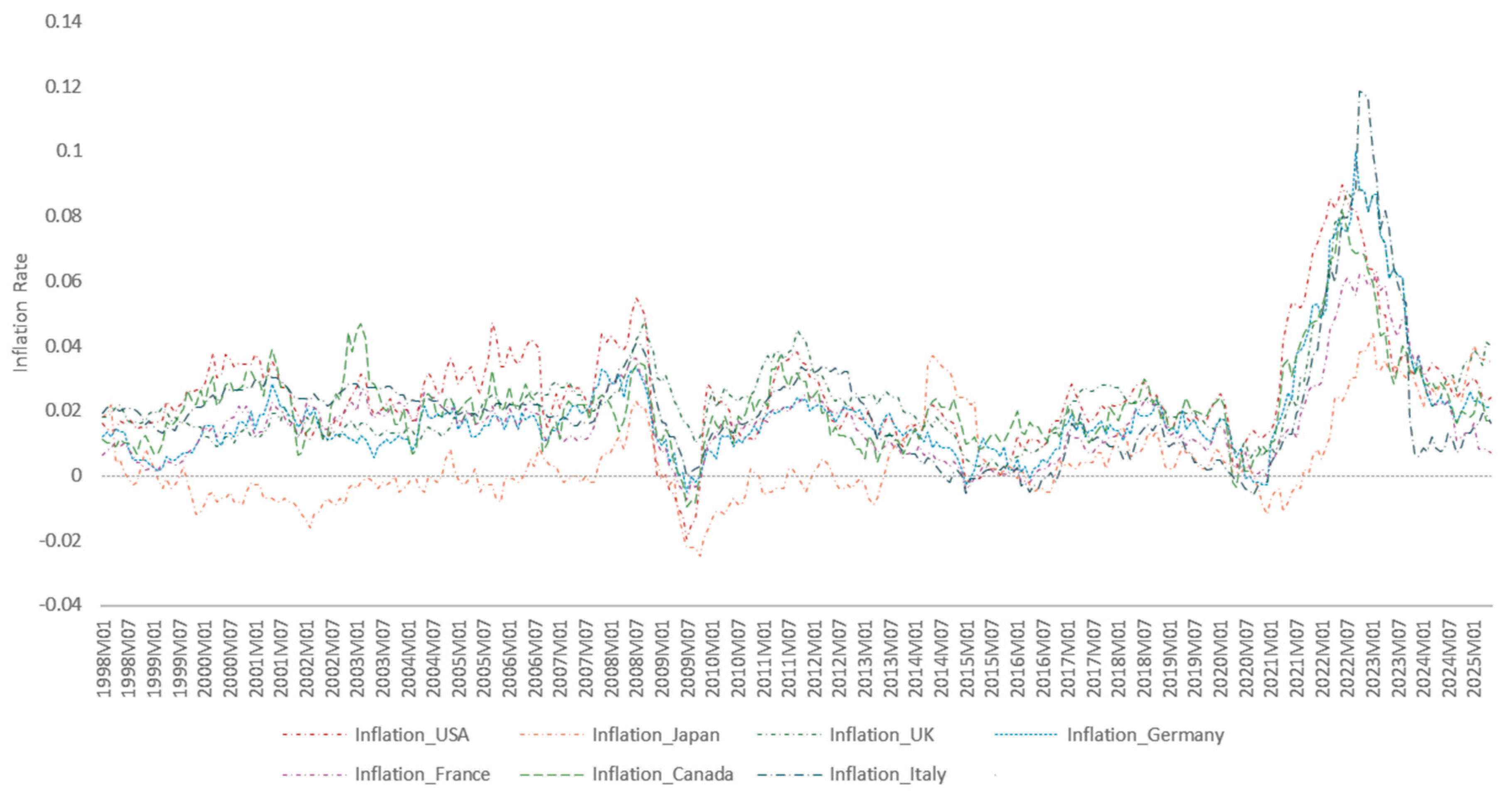
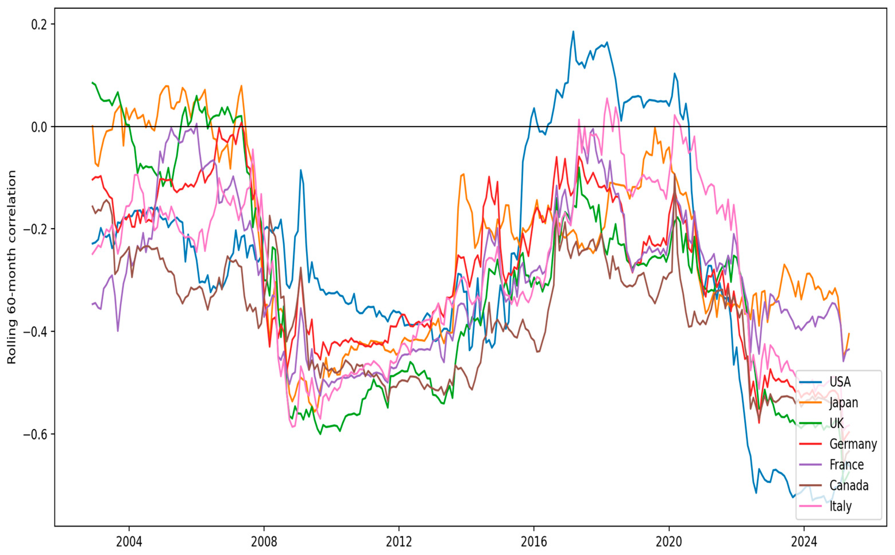
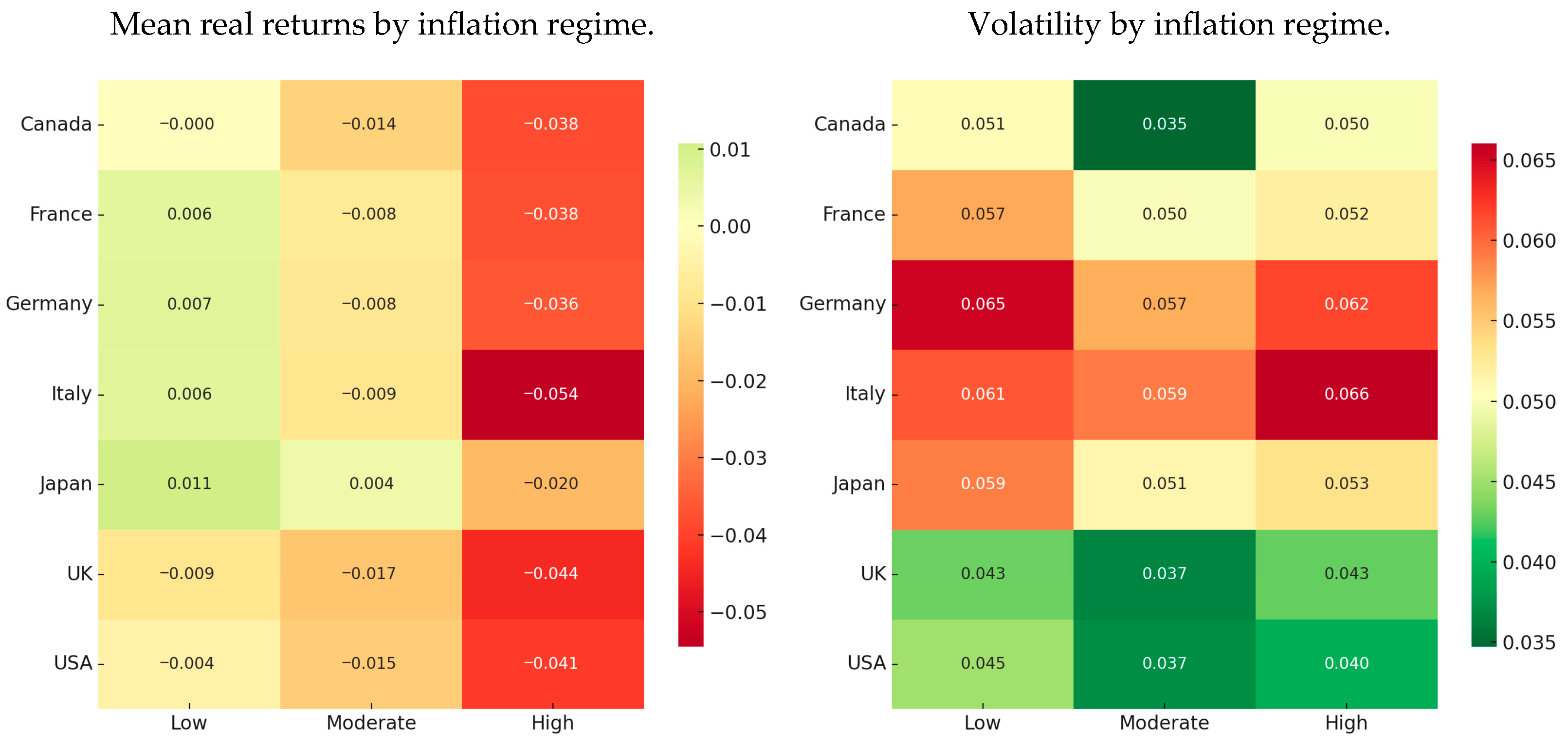
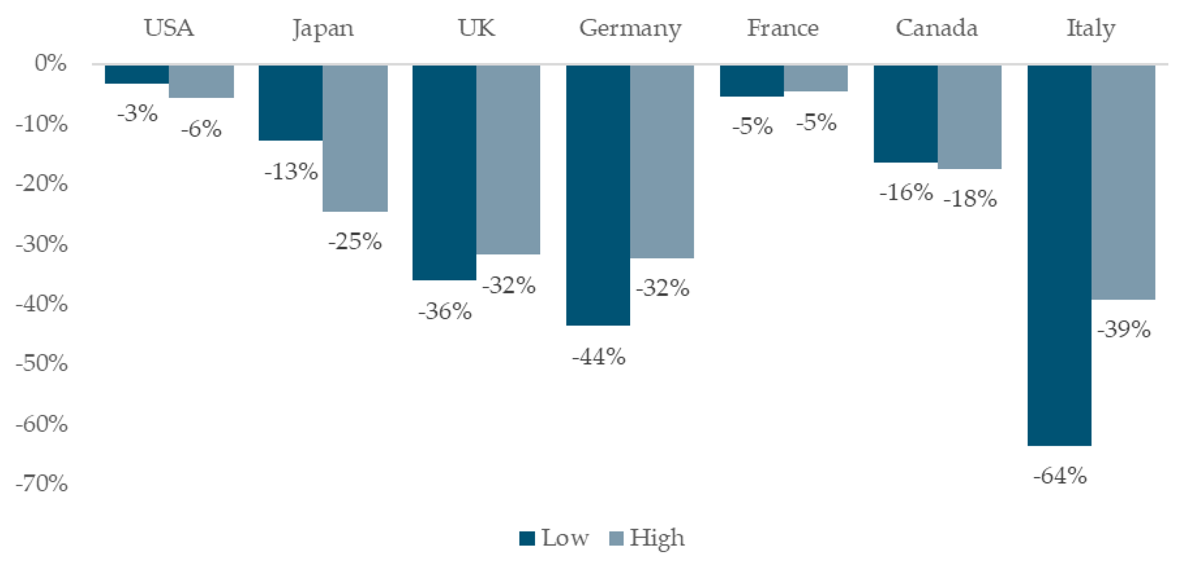
Furthermore, time-varying rolling correlations, shown in Appendix A, offer additional descriptive evidence of regime-dependent co-movement between inflation and equity returns. Figure 2 also highlights how G7 equity markets differ in their responses to inflation regimes. Italy and the United Kingdom exhibit the steepest deterioration in stock returns when inflation shifts from low to high regimes, with Italy uniquely experiencing a simultaneous rise in volatility. France and Germany also suffer substantial return losses under high inflation, although volatility does not intensify further. This suggests that some adjustment occurs through risk repricing rather than heightened market instability. By contrast, Japan emerges as the most resilient market, with returns declining only modestly and volatility even falling under high inflation. Canada and the United States occupy an intermediate position, with consistent return erosion but broadly stable volatility. This may reflect the greater depth and liquidity of their financial markets.

These findings demonstrate that the impact of inflation shocks is nonlinear and state-dependent. In low regimes, stock markets can absorb inflationary pressures with minimal damage, while in high regimes, the same shocks trigger disproportionate declines in returns and, in some cases, increased volatility. Linear impulse response methods would average out these contrasting dynamics, thereby masking the fragility of some markets and overestimating the resilience of others. Nonlinear local projections (NLPs) provide a more suitable framework because they enable impulse responses to vary across regimes without imposing symmetry or parameter constancy. This flexibility captures the asymmetric amplification of shocks in high-inflation environments and the dampening effects observable in low-inflation states. Moreover, NLPs enable transparent accounting for cross-country heterogeneity, revealing that Japan’s resilience and Italy’s vulnerability are not anomalies but systematic, nonlinear features of the inflation–stock market relationship.

To capture these conditional dynamics, we extend the analysis using a nonlinear local projection framework that distinguishes between high- and low-inflation regimes and between positive and negative inflation shocks. This approach allows us to assess whether the cross-country vulnerability patterns observed in the average response persist, diminish, or reverse once we condition on the inflation state and shock direction, thereby refining both the investor and policy implications derived from the baseline model. Moreover, we estimate the high- and low-inflation and positive- and negative-shock specifications separately rather than jointly. Estimating these models separately avoids collinearity arising from overlapping states and permits a direct interpretation of the resulting impulse responses. Each specification isolates a single dimension of nonlinearity while preserving comparability across countries and horizons.

4. The State-Dependent and Sign-Dependent Local Projection Dynamics

4.1. High- vs. Low-Inflation Regime Responses

To examine whether the equity–inflation relationship varies across macroeconomic conditions, we extend the baseline local projection framework to a state-dependent setting. We estimate impulse response functions conditional on the prevailing inflation regime, classified as high or low based on whether the year-on-year CPI inflation rate exceeds its sample median. A high-inflation regime is flagged when lagged month-on-month inflation exceeds the country-specific median: $1_t^{HI}=1\left\{∆{\pi }_{t-1}^c>median\left(∆{\pi }^c\right)\right\}$. Low-inflation months are the complement. For each horizon h = 0, 1,…, 12 and each country c, we estimate

$$∆r_{t+h}^c={\alpha }_h^c+\underset{low}{\underbrace{{\beta }_h^{L,c}}}.{\epsilon }_t^{\pi ,c}+\underset{high}{\underbrace{{\beta }_h^{H,c}}}.{\epsilon }_t^{\pi ,c}.1_t^{HI}+{\sum }_{j=1}^n{\gamma }_{h,j}^c{\epsilon }_{t-j}^{\pi ,c}+{\sum }_{j=1}^n{\delta }_{h,j}^c{∆r}_{t-j}^c+u_{t+h}^c$$

(2)

• ${\beta }_h^{L,c}$: impulse response under low inflation.
• ${\beta }_h^{H,c}$: additional effect when the same shock hits in a high-inflation month; the total high-regime response is ${\beta }_h^{L,c}+{\beta }_h^{H,c}$.

The choice of the sample median as a regime threshold is motivated by several considerations. First, the median is robust to outliers and provides a stable, data-driven benchmark that aligns with the implicit inflation anchor over the full sample for most G7 economies. Second, it ensures a balanced number of observations across regimes, thereby supporting estimation precision in nonlinear specifications. A limitation of this approach is that it abstracts from time-varying or country-specific threshold dynamics. Alternative regime definitions—such as quantile-based thresholds, historical means, time-varying breakpoints, or pre- and post-crisis subsamples—are commonly used in the literature and could be explored. However, existing evidence suggests that while magnitudes may vary, the qualitative patterns of regime-dependent amplification and cross-country differences remain robust across such classifications. Accordingly, the regime-dependent results should be interpreted as conditional on this classification and as descriptive evidence of state-dependent behavior rather than as estimates tied to a unique or optimal inflation threshold.

Table 5. High- vs. low-inflation regime IRFs results.

	USA		Japan		UK		Germany		France		Canada		Italy
h	beta_low	beta_high	beta_low	beta_high	beta_low	beta_high	beta_low	beta_high	beta_low	beta_high	beta_low	beta_high	beta_low	beta_high
0	−0.0019	−0.0076 **	−0.0158	−0.0130	−0.0019	−0.0033	−0.0213	−0.0066	0.0037	−0.0020	−0.0075	−0.0005	−0.0290 *	−0.0150
1	0.0000	−0.0080 ***	−0.0189	−0.0208 **	−0.0235 **	−0.0256	−0.0318 **	−0.0178	−0.0025	−0.0017	−0.0207 ***	−0.0279 ***	−0.0440 ***	−0.0309 *
2	−0.0039	−0.0057	−0.0267 **	−0.0329 ***	−0.0260 **	−0.0291	−0.0084	0.0040	−0.0034	0.0030	−0.0212 ***	−0.0270 ***	−0.0396 ***	−0.0283 ***
3	0.0004	−0.0018	−0.0258 **	−0.0319 ***	−0.0134	−0.0166	−0.0489 ***	−0.0364 ***	−0.0039	−0.0116 **	−0.0110	−0.0146 **	−0.0336 **	−0.0236
4	0.0032	0.0003	−0.0221	−0.0316 **	−0.0299 ***	−0.0333	−0.0533 ***	−0.0391 **	−0.0025	−0.0070 *	−0.0339 ***	−0.0366 ***	−0.0447 ***	−0.0355 **
5	−0.0070	−0.0006	−0.0030	−0.0171	−0.0370 **	−0.0378	−0.0291 *	−0.0179	−0.0088 **	−0.0057 *	−0.0132	−0.0168 **	−0.0563 ***	−0.0442 ***
6	−0.0086 **	−0.0058 *	0.0086	−0.0068	−0.0364 ***	−0.0369	−0.0471 ***	−0.0394 ***	−0.0095 ***	−0.0072 *	−0.0116	−0.0115	−0.0650 ***	−0.0474 **
7	−0.0071 ***	−0.0072 *	−0.0134	−0.0214	−0.0262 *	−0.0255	−0.0166	−0.0037	−0.0026	0.0023	−0.0045	−0.0058	−0.0598 ***	−0.0401 **
8	−0.0032	−0.0059	0.0018	−0.0063	−0.0355 ***	−0.0310	−0.0530 ***	−0.0417 ***	−0.0124 **	−0.0037	−0.0060	−0.0100	−0.0333 *	−0.0084
9	−0.0010	−0.0066	−0.0236 **	−0.0330 **	−0.0197	−0.0118	−0.0327 **	−0.0305 ***	−0.0076 *	0.0019	−0.0115	−0.0104	−0.0531 ***	−0.0269 **
10	−0.0007	−0.0022	0.0003	−0.0117	−0.0375 **	−0.0248	−0.0232 *	−0.0175	−0.0079 *	0.0029	−0.0077	−0.0045	−0.0562 ***	−0.0287 **
11	−0.0074 ***	−0.0013	0.0021	−0.0175 *	−0.0391 ***	−0.0228	−0.0368 **	−0.0386 ***	0.0019	−0.0097 *	−0.0046	−0.0005	−0.0652 ***	−0.0367 **
12	0.0046	−0.0054	0.0078	−0.0026	−0.0355 ***	−0.0195	−0.0345 **	−0.0381 ***	0.0011	−0.0087 **	−0.0111	−0.0095	−0.0564 ***	−0.0266 **

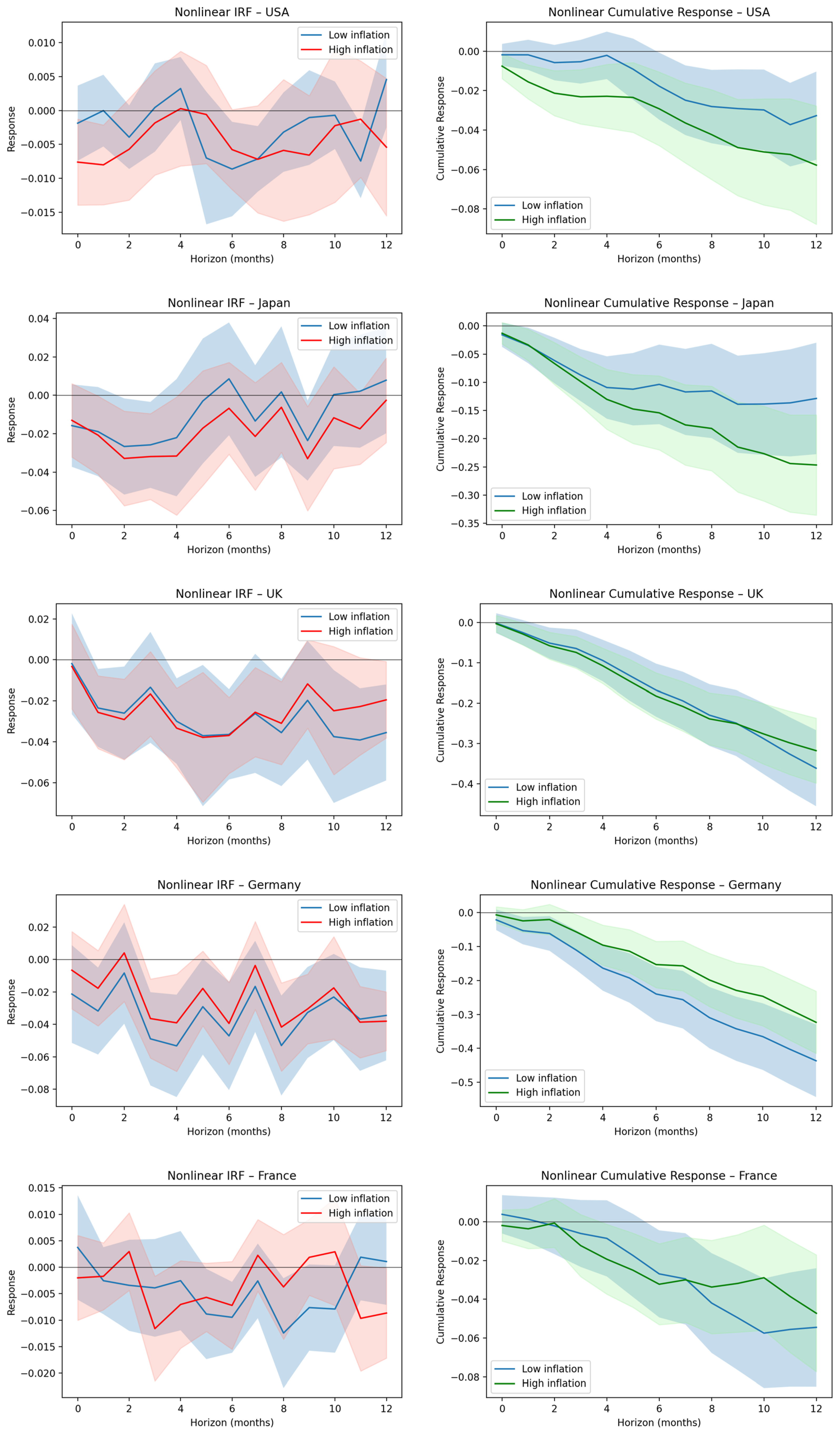
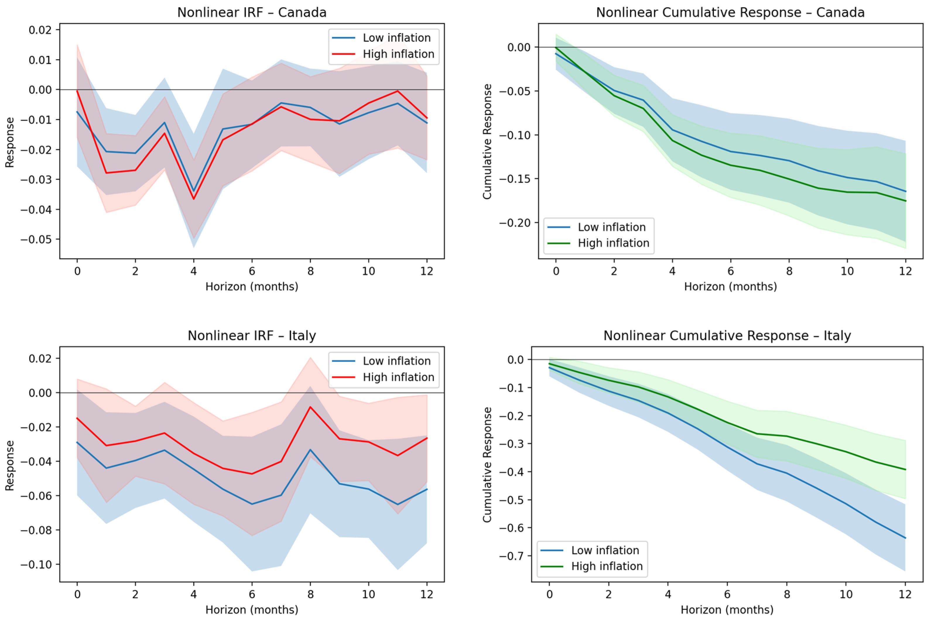
Significance: * for p < 0.1, ** for p < 0.05, and *** for p < 0.01.

and Figure 3 show that, at short horizons, equity losses are generally larger when inflation is already elevated. At h = 1, high-inflation impulse responses are more negative than their low-inflation counterparts in most G7 economies. The regime gap is modest in the United States, indicating limited state amplification, but pronounced in Canada, Japan, and the United Kingdom, where equity markets reprice inflation risk more aggressively under elevated inflation. France stands out as an outlier, with responses that are statistically insignificant in both regimes. Italy departs from the dominant pattern, exhibiting larger short-run losses in low-inflation environments, suggesting vulnerability even during periods of price stability.

Persistence dynamics, also illustrated in Figure 3, differ markedly across countries. In the United States and France, regime-conditional impulse responses revert toward zero within three months, consistent with rapid expectation anchoring. In contrast, Germany, Japan, the United Kingdom, and Italy exhibit delayed troughs around months two to three, indicating multi-stage repricing when inflation shocks occur under adverse conditions. Canada displays the most front-loaded response, with a sharp initial drawdown followed by gradual easing that remains negative over extended horizons.

Cumulative responses reported in

Table 6. High- vs. low-inflation regime cumulative responses.

	USA		Japan		UK		Germany		France		Canada		Italy
h	cum_low	cum_high	cum_low	cum_high	cum_low	cum_high	cum_low	cum_high	cum_low	cum_high	cum_low	cum_high	cum_low	cum_high
0	−0.0019	−0.0076 **	−0.0158	−0.0130	−0.0019	−0.0033	−0.0213	−0.0066	0.0037	−0.0020	−0.0075	−0.0005	−0.0290 *	−0.0150
1	−0.0019	−0.0156 ***	−0.0347 **	−0.0338 **	−0.0253	−0.0289 **	−0.0531 ***	−0.0244	0.0012	−0.0037	−0.0282 **	−0.0284 ***	−0.0731 ***	−0.0459 **
2	−0.0058	−0.0213 ***	−0.0614 ***	−0.0667 ***	−0.0513 ***	−0.0580 ***	−0.0615 **	−0.0204	−0.0022	−0.0007	−0.0494 ***	−0.0553 ***	−0.1126 ***	−0.0742 ***
3	−0.0054	−0.0232 ***	−0.0872 ***	−0.0986 ***	−0.0648 ***	−0.0746 ***	−0.1104 ***	−0.0568 **	−0.0061	−0.0123	−0.0604 ***	−0.0699 ***	−0.1462 ***	−0.0977 ***
4	−0.0021	−0.0229 ***	−0.1092 ***	−0.1302 ***	−0.0947 ***	−0.1079 ***	−0.1637 ***	−0.0959 ***	−0.0086	−0.0194 **	−0.0943 ***	−0.1065 ***	−0.1909 ***	−0.1332 ***
5	−0.0091	−0.0235 ***	−0.1122 ***	−0.1474 ***	−0.1317 ***	−0.1457 ***	−0.1928 ***	−0.1137 ***	−0.0175	−0.0250 **	−0.1075 ***	−0.1233 ***	−0.2472 ***	−0.1774 ***
6	−0.0178 **	−0.0292 ***	−0.1037 ***	−0.1541 ***	−0.1682 ***	−0.1826 ***	−0.2399 ***	−0.1532 ***	−0.0269 **	−0.0322 ***	−0.1191 ***	−0.1348 ***	−0.3122 ***	−0.2247 ***
7	−0.0249 ***	−0.0364 ***	−0.1171 ***	−0.1756 ***	−0.1943 ***	−0.2082 ***	−0.2565 ***	−0.1569 ***	−0.0295 **	−0.0300 ***	−0.1236 ***	−0.1405 ***	−0.3720 ***	−0.2649 ***
8	−0.0281 ***	−0.0423 ***	−0.1153 ***	−0.1818 ***	−0.2298 ***	−0.2391 ***	−0.3096 ***	−0.1986 ***	−0.0419 ***	−0.0337 ***	−0.1295 ***	−0.1505 ***	−0.4053 ***	−0.2733 ***
9	−0.0291 ***	−0.0489 ***	−0.1389 ***	−0.2148 ***	−0.2495 ***	−0.2509 ***	−0.3423 ***	−0.2291 ***	−0.0495 ***	−0.0318 **	−0.1410 ***	−0.1609 ***	−0.4584 ***	−0.3002 ***
10	−0.0298 ***	−0.0511 ***	−0.1386 ***	−0.2265 ***	−0.2870 ***	−0.2757 ***	−0.3654 ***	−0.2466 ***	−0.0574 ***	−0.0289 **	−0.1488 ***	−0.1654 ***	−0.5146 ***	−0.3289 ***
11	−0.0373 ***	−0.0524 ***	−0.1365 ***	−0.2440 ***	−0.3261 ***	−0.2985 ***	−0.4022 ***	−0.2853 ***	−0.0555 ***	−0.0385 ***	−0.1534 ***	−0.1659 ***	−0.5798 ***	−0.3656 ***
12	−0.0327 ***	−0.0578 ***	−0.1286 **	−0.2466 ***	−0.3616 ***	−0.3180 ***	−0.4367 ***	−0.3233 ***	−0.0544 ***	−0.0472 ***	−0.1645 ***	−0.1754 ***	−0.6362 ***	−0.3922 ***

Significance: * for p < 0.1, ** for p < 0.05, and *** for p < 0.01.

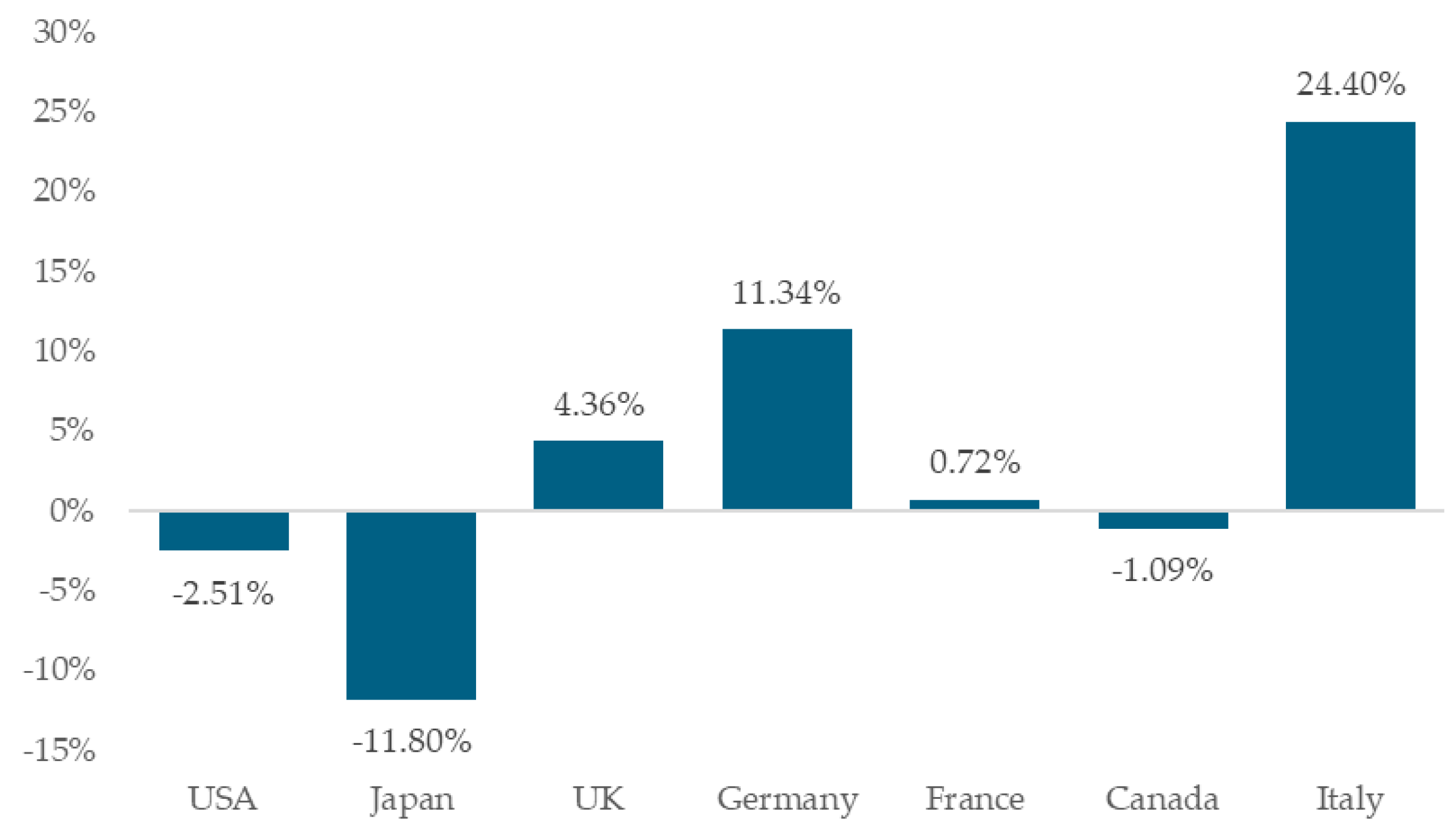
and Figure 4 reinforce these distinctions. By twelve months, Italy, Germany, and the United Kingdom experience larger cumulative losses following shocks that occur in low-inflation regimes, whereas Japan and Canada exhibit deeper cumulative drawdowns under high inflation. The United States and France record comparatively small cumulative losses in both regimes. The regime gaps summarized in Figure 5 highlight this heterogeneity. Italy shows the largest positive gap, indicating greater sensitivity to low inflation, while Japan shows a negative gap, signaling greater vulnerability to elevated inflation. The remaining countries exhibit more moderate asymmetries.

4.2. Positive vs. Negative Shock Asymmetries

To examine asymmetry by shock direction, we next estimate a second set of state-dependent local projections conditioned on the sign of the inflation surprise. Observations are classified into positive and negative regimes based on whether the month-on-month CPI surprise is above or below zero. This partition distinguishes periods during which inflation accelerates from those during which it decelerates. We defined a dummy that equals one for upside (positive) surprises: $1_t^{+}=1\left\{{\epsilon }_t^{\pi ,c}>0\right\},1_t^{-}=1-1_t^{+}$. Negative surprises are the complement. Because the shock is σ-scaled, the positive and negative states have equal unconditional variance. For each horizon h = 0, 1,…, 12 we estimate, country by country,

$$∆r_{t+h}^c={\alpha }_h^c+{\beta }_h^{-c}.{\epsilon }_t^{\pi ,c}+{\beta }_h^{+c}.{\epsilon }_t^{\pi ,c}.1_t^{+}+{\sum }_{j=1}^n{\gamma }_{h,j}^c{\epsilon }_{t-j}^{\pi ,c}+{\sum }_{j=1}^n{\delta }_{h,j}^c{∆r}_{t-j}^c+u_{t+h}^c$$

(3)

${\beta }_h^{-}$ captures the response to a negative surprise. ${\beta }_h^{+}$ is the incremental effect when the shock is positive, so the complete positive-surprise response is ${\beta }_h^{-}+{\beta }_h^{+}$.

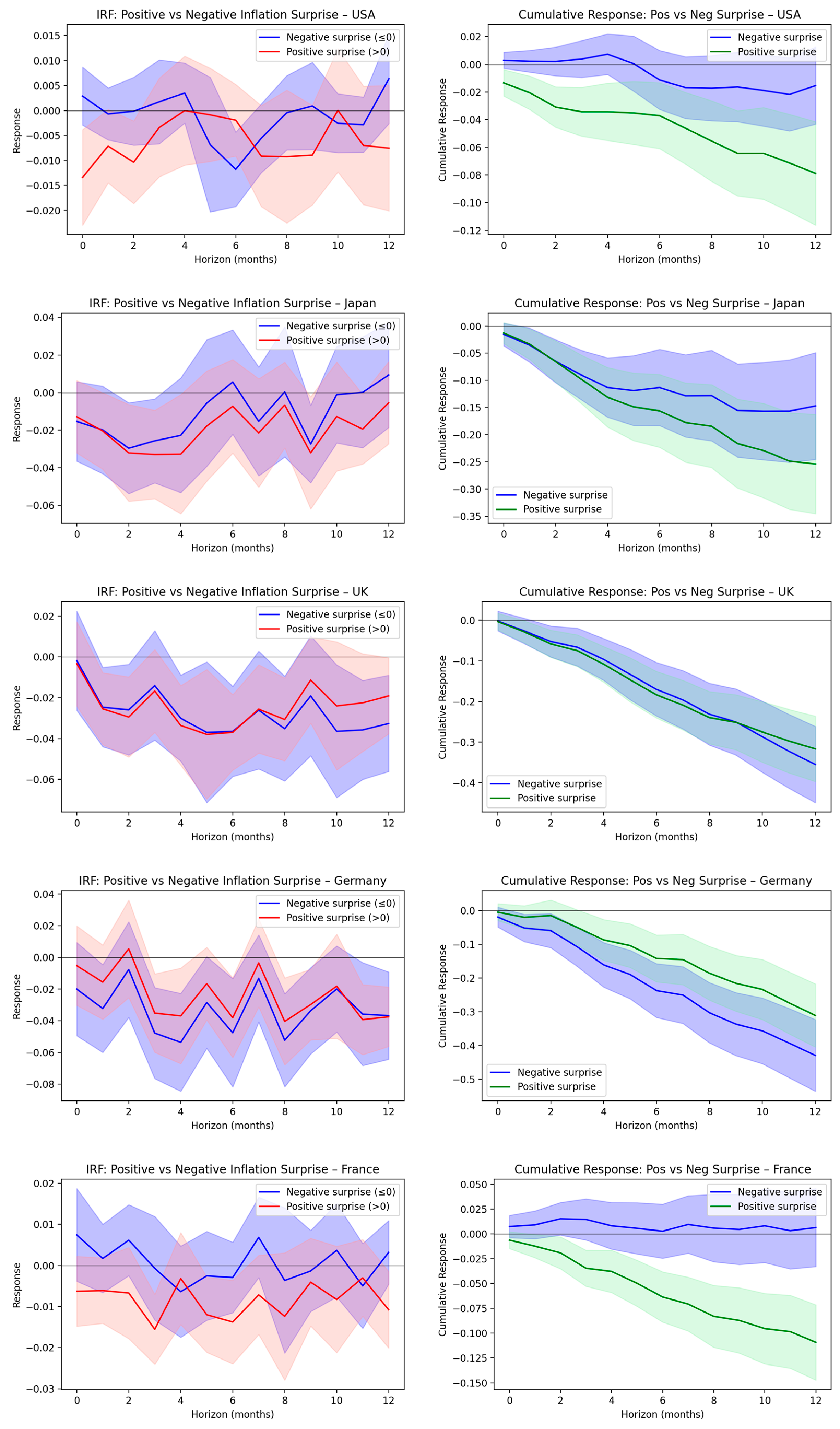
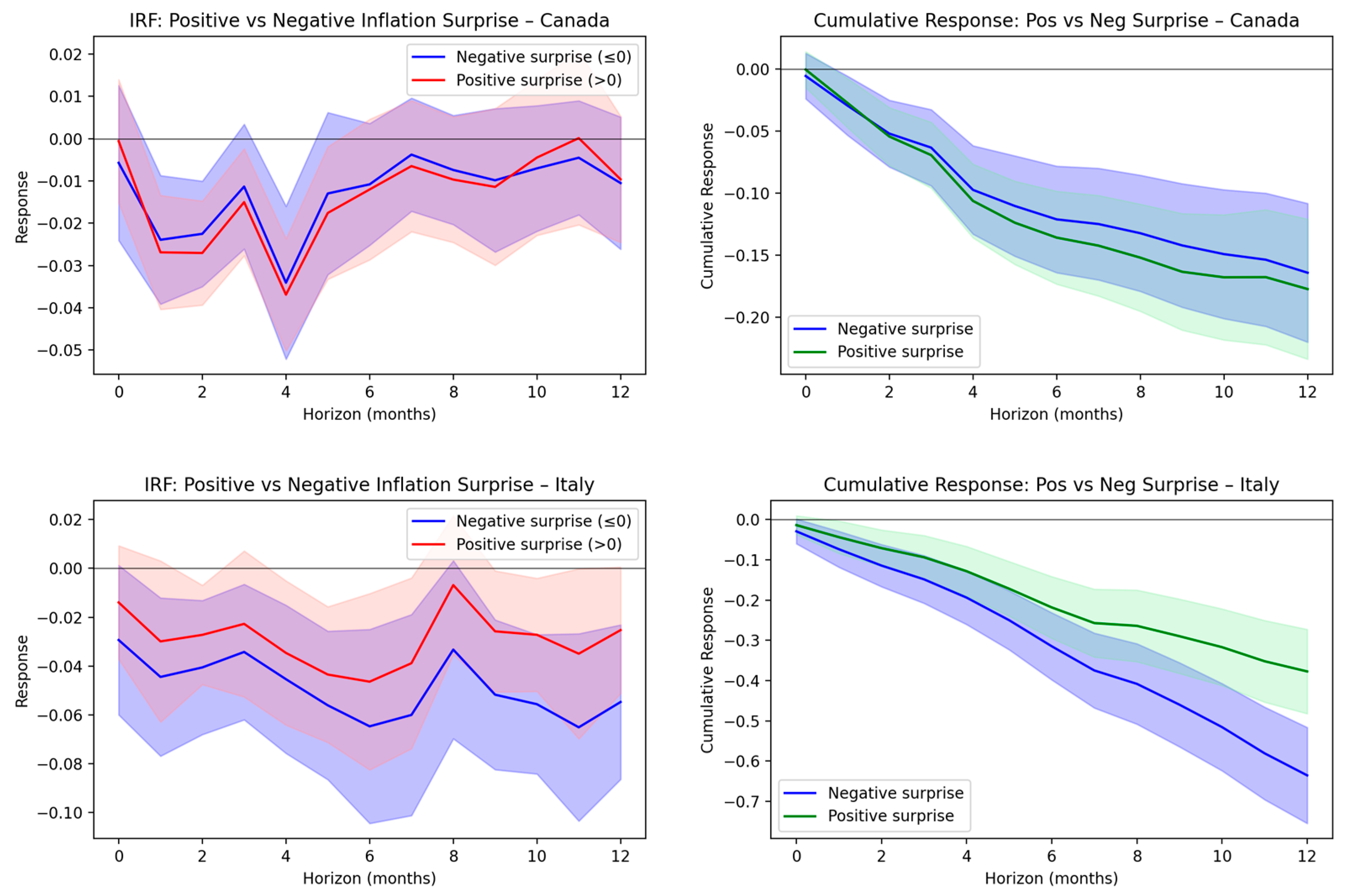
The positive-versus-negative specification reveals an even starker asymmetry than the high-versus-low-inflation exercise: most equity markets penalize upside inflation surprises while largely ignoring downside surprises. Figure 6 and

Table 7. Positive vs. negative inflation surprises IRFs results.

	USA		Japan		UK		Germany		France		Canada		Italy
h	beta_neg	beta_pos	beta_neg	beta_pos	beta_neg	beta_pos	beta_neg	beta_pos	beta_neg	beta_pos	beta_neg	beta_pos	beta_neg	beta_pos
0	0.0029	−0.0134 ***	−0.0154	−0.0129	−0.0018	−0.0034	−0.0200	−0.0052	0.0074	−0.0063	−0.0057	−0.0006	−0.0293 *	−0.0139
1	−0.0007	−0.0071 **	−0.0199 *	−0.0205 **	−0.0246 **	−0.0254 ***	−0.0323 **	−0.0156	0.0017	−0.0061	−0.0239 ***	−0.0269 ***	−0.0445 ***	−0.0299 *
2	−0.0001	−0.0104 **	−0.0296 **	−0.0321 **	−0.0259 **	−0.0295 ***	−0.0077	0.0054	0.0061	−0.0067	−0.0225 ***	−0.0270 ***	−0.0406 ***	−0.0272 ***
3	0.0017	−0.0034	−0.0257 **	−0.0329 ***	−0.0140	−0.0167	−0.0479 ***	−0.0352 ***	−0.0007	−0.0155 ***	−0.0113	−0.0150 **	−0.0342 **	−0.0227
4	0.0035	0.0000	−0.0227	−0.0328 **	−0.0300 ***	−0.0336 ***	−0.0536 ***	−0.0369 **	−0.0064	−0.0032	−0.0341 ***	−0.0369 ***	−0.0454 ***	−0.0346 **
5	−0.0068	−0.0009	−0.0056	−0.0178	−0.0370 **	−0.0379 **	−0.0285 *	−0.0166	−0.0025	−0.0120 **	−0.0130	−0.0176 **	−0.0561 ***	−0.0435 ***
6	−0.0118 ***	−0.0019	0.0056	−0.0073	−0.0365 ***	−0.0369 ***	−0.0476 ***	−0.0381 ***	−0.0029	−0.0138 ***	−0.0108	−0.0120	−0.0647 ***	−0.0464 **
7	−0.0055	−0.0091 *	−0.0153	−0.0215	−0.0260 *	−0.0255 **	−0.0133	−0.0035	0.0068	−0.0072	−0.0038	−0.0065	−0.0600 ***	−0.0388 **
8	−0.0004	−0.0092	0.0004	−0.0066	−0.0352 ***	−0.0306 ***	−0.0523 ***	−0.0404 ***	−0.0037	−0.0124	−0.0074	−0.0097	−0.0333 *	−0.0068
9	0.0009	−0.0089 *	−0.0274 ***	−0.0321 **	−0.0191	−0.0113	−0.0337 **	−0.0298 ***	−0.0014	−0.0041	−0.0098	−0.0114	−0.0517 ***	−0.0258 **
10	−0.0025	0.0000	−0.0011	−0.0127	−0.0365 **	−0.0240	−0.0200	−0.0182	0.0037	−0.0083	−0.0070	−0.0045	−0.0556 ***	−0.0272 **
11	−0.0028	−0.0070	0.0001	−0.0194 **	−0.0358 ***	−0.0224 *	−0.0358 **	−0.0393 ***	−0.0050	−0.0030	−0.0045	0.0001	−0.0651 ***	−0.0350 *
12	0.0064	−0.0075	0.0093	−0.0054	−0.0326 ***	−0.0190 **	−0.0368 ***	−0.0375 ***	0.0032	−0.0108 **	−0.0105	−0.0096	−0.0547 ***	−0.0253 *

Significance: * for p < 0.1, ** for p < 0.05, and *** for p < 0.01.

and

Table 8. Positive vs. negative inflation surprises cumulative responses.

	USA		Japan		UK		Germany		France		Canada		Italy
h	cum_neg	cum_pos	cum_neg	cum_pos	cum_neg	cum_pos	cum_neg	cum_pos	cum_neg	cum_pos	cum_neg	cum_pos	cum_neg	cum_pos
0	0.0029	−0.0134 ***	−0.0154	−0.0129	−0.0018	−0.0034	−0.0200	−0.0052	0.0074	−0.0063	−0.0057	−0.0006	−0.0293 **	−0.0139
1	0.0022	−0.0205 ***	−0.0352 **	−0.0333 **	−0.0265 *	−0.0288 **	−0.0523 **	−0.0208	0.0091	−0.0124 **	−0.0296 **	−0.0274 ***	−0.0738 ***	−0.0439 **
2	0.0021	−0.0309 ***	−0.0648 ***	−0.0654 ***	−0.0523 ***	−0.0582 ***	−0.0600 **	−0.0154	0.0153 *	−0.0191 **	−0.0521 ***	−0.0545 ***	−0.1144 ***	−0.0711 ***
3	0.0038	−0.0343 ***	−0.0905 ***	−0.0984 ***	−0.0663 ***	−0.0749 ***	−0.1079 ***	−0.0506 *	0.0146	−0.0347 ***	−0.0634 ***	−0.0695 ***	−0.1486 ***	−0.0938 ***
4	0.0073	−0.0343 ***	−0.1132 ***	−0.1311 ***	−0.0964 ***	−0.1085 ***	−0.1615 ***	−0.0876 ***	0.0082	−0.0379 ***	−0.0975 ***	−0.1064 ***	−0.1940 ***	−0.1284 ***
5	0.0005	−0.0352 ***	−0.1188 ***	−0.1489 ***	−0.1333 ***	−0.1464 ***	−0.1900 ***	−0.1042 ***	0.0056	−0.0499 ***	−0.1104 ***	−0.1239 ***	−0.2501 ***	−0.1719 ***
6	−0.0113	−0.0371 ***	−0.1132 ***	−0.1563 ***	−0.1698 ***	−0.1833 ***	−0.2376 ***	−0.1423 ***	0.0027	−0.0636 ***	−0.1212 ***	−0.1359 ***	−0.3148 ***	−0.2183 ***
7	−0.0168	−0.0462 ***	−0.1285 ***	−0.1777 ***	−0.1959 ***	−0.2089 ***	−0.2508 ***	−0.1458 ***	0.0095	−0.0708 ***	−0.1250 ***	−0.1424 ***	−0.3748 ***	−0.2572 ***
8	−0.0173	−0.0554 ***	−0.1282 ***	−0.1844 ***	−0.2310 ***	−0.2395 ***	−0.3032 ***	−0.1862 ***	0.0058	−0.0832 ***	−0.1324 ***	−0.1521 ***	−0.4081 ***	−0.2640 ***
9	−0.0164	−0.0644 ***	−0.1556 ***	−0.2164 ***	−0.2501 ***	−0.2508 ***	−0.3369 ***	−0.2160 ***	0.0045	−0.0873 ***	−0.1422 ***	−0.1635 ***	−0.4598 ***	−0.2898 ***
10	−0.0189	−0.0643 ***	−0.1567 ***	−0.2292 ***	−0.2865 ***	−0.2748 ***	−0.3568 ***	−0.2342 ***	0.0082	−0.0956 ***	−0.1492 ***	−0.1679 ***	−0.5154 ***	−0.3170 ***
11	−0.0217	−0.0713 ***	−0.1565 ***	−0.2486 ***	−0.3223 ***	−0.2972 ***	−0.3927 ***	−0.2735 ***	0.0032	−0.0986 ***	−0.1537 ***	−0.1678 ***	−0.5805 ***	−0.3520 ***
12	−0.0154	−0.0788 ***	−0.1472 ***	−0.2540 ***	−0.3549 ***	−0.3163 ***	−0.4294 ***	−0.3111 ***	0.0064	−0.1094 ***	−0.1642 ***	−0.1774 ***	−0.6353 ***	−0.3772 ***

Significance: * for p < 0.1, ** for p < 0.05, and *** for p < 0.01.

show that, at short horizons, upside inflation surprises lead to larger immediate losses across most markets, particularly in the United States, Japan, the United Kingdom, and Canada. In contrast, Germany and Italy respond more strongly to downside surprises, indicating that disinflation in these economies is interpreted less as monetary relief and more as a signal of weakening demand. France again exhibits minimal sensitivity to either shock direction.

At medium horizons, cumulative responses diverge further. As shown in

Table 9. Summary of sign leadership by country and horizon.

Country	Short-Term (h = 0)	Medium-Term (h = 6)	Long-Term (h = 12)	Asymmetry Direction
USA	Positive	Positive	Positive	Positive shock driven at all horizons
Japan	Negative	Positive	Positive	Shift from negative to positive dominance
UK	Positive	Positive	Negative	Positive early, turns negative long-term
Germany	Negative	Negative	Negative	Negative shock driven throughout
France	None	Negative	Positive	No clear short-term effect, shifts over time
Canada	None	Positive	Positive	Positive shock in the medium and long term
Italy	Negative	Negative	Negative	Negative shock driven at all horizons

, positive shocks dominate cumulative losses in the United States, Japan, Canada, and France, consistent with a persistent tightening-path premium embedded in valuations. Negative shocks dominate in Germany, Italy, and the United Kingdom, where disinflationary news appears to raise equity risk premia by signaling macroeconomic fragility rather than easing financial conditions.

At longer horizons, the divergence becomes sharper. By h = 12, cumulative losses from negative shocks exceed those from positive shocks in Italy, Germany, and the United Kingdom, while positive shocks remain more damaging in the United States, Japan, France, and Canada.

Table 9 compares and summarizes the relative dominance of positive versus negative inflation shocks in driving equity market responses across G7 economies. Across many G7 markets, positive inflation surprises generate larger and more persistent declines in equity returns than negative surprises of equivalent size. This asymmetry emerges early, in the case of the United States and the United Kingdom, where the immediate penalty from positive shocks is more than double that from negative shocks at short horizons. However, Italy is an exception, where the negative shock impact is actually larger in magnitude, and Canada’s short-term asymmetry is weaker.

In the medium term, the negative impact of positive shocks remains economically and statistically significant across most markets, with particularly deep declines in Italy, Germany, and the UK. Adverse shocks, in contrast, often fade to insignificance or turn marginally positive—as in France and Japan—but persist in structurally fragile economies such as Italy and, to a lesser extent, the UK. Over a one-year horizon, the divergence between shock types becomes sharper. Positive shocks continue to dominate, producing substantial cumulative drawdowns in Italy, Germany, Japan, and Canada. Negative shocks remain muted in some markets. The lack of response to negative surprises suggests that investors either doubt the persistence of disinflationary pressures, view them as growth-negative, or regard them as signs of severe macroeconomic distress rather than as relief from inflationary pressures. All these perceived perceptions neutralize potential valuation gains.

In detail, the evidence establishes a double asymmetry in the transmission of inflation shocks to equity markets. Equity losses depend not only on the size of the shock but also on the inflation regime and the direction of the surprise. In some economies, inflation shocks are most damaging when inflation is already high. In others, surprises during periods of price stability generate larger cumulative losses. Similarly, positive inflation surprises dominate in some markets, while negative surprises dominate in others. This asymmetric pattern aligns with prior evidence that markets penalize inflationary news disproportionately (Cochrane, 2022a, 2022b, 2022c; Gürkaynak et al., 2005). For policymakers, this asymmetry underscores the dual challenge of anchoring inflation expectations while maintaining financial stability, as the same CPI surprise can elicit vastly different market consequences depending on its sign and the prevailing macroeconomic context. For global investors, these findings highlight the necessity of regime- and sign-aware risk management, tailoring hedging strategies to the specific vulnerabilities of each market.

5. Joint Regime–Sign Asymmetries in the Inflation–Equity Nexus

Based on the separate analyses of state dependence (high- vs. low-inflation regimes) and sign asymmetry (positive vs. negative surprises), we now integrate the two dimensions into a unified four-regime framework: high-positive, high-negative, low-positive, and low-negative shocks. This joint specification allows us to examine not only whether equity markets react more strongly when inflation is already elevated, but also whether the direction of the surprise amplifies or mitigates those regime effects. This approach suggests that when inflation is high, unexpected increases in inflation can lead to significant financial losses. In contrast, when inflation is low, decreases in inflation may have little or no negative impact. By examining how different states and signs interact, this analysis provides a clearer view of how inflation affects the stock market. It also highlights the varying reactions of the G7 economies.

We estimate for each horizon and country by country the following equation:

$$\mathsf{\Delta }{r}_{t+h}={\beta }_h^{L-}{D}_t^{L-}{\epsilon }_t+{\beta }_h^{L+}{D}_t^{L+}{\epsilon }_t+{\beta }_h^{H+}{D}_t^{H+}{\epsilon }_t+{\beta }_h^{H-}{D}_t^{H-}{\epsilon }_t+{\sum }_{j=1}^n{\gamma }_{h,j}^c{\epsilon }_{t-j}^{\pi ,c}+{\sum }_{j=1}^n{\delta }_{h,j}^c\mathsf{\Delta }{r}_{t-j}^c+u_{t+h}^c$$

(4)

where: $D_t^{L-}=(1-1_t^{HI})(1-1_t^{+})$, $D_t^{H+}=1_t^{HI}{1}_t^{+}$, $D_t^{H-}=1_t^{HI}(1-1_t^{+})$, $D_t^{L+}=(1-1_t^{HI})1_t^{+}$ and $D_t^{L-}+D_t^{L+}+D_t^{H-}+D_t^{H+}=1$.

• $1_t^{HI}=1\left\{{∆\pi }_{t-1}^c>median\left(∆{\pi }^c\right)\right\}$ indicates the high-inflation regime.
• $1_t^{+}=1\left\{{\epsilon }_t^{\pi ,c}>0\right\}$ indicates a positive inflation surprise.
• ${\beta }_h^{L+,c}$: Response in a low-inflation, positive-shock regime.
• ${\beta }_h^{L-,c}$: Response in a low-inflation, negative-shock regime.
• ${\beta }_h^{H+,c}$: Response in a high-inflation, positive-shock regime.
• ${\beta }_h^{H-,c}$: Response in a high-inflation, negative-shock regime.

We eliminated the constant term to avoid multicollinearity. This specification allows a complete decomposition of the response into four distinct regimes, based on both the prevailing inflation environment and the sign of the inflation surprise.

Our results, displayed in

Table 10. Low regime–sign cumulative responses.

	USA		Japan		UK		Germany		France		Canada		Italy
h	low_neg	low_pos	low_neg	low_pos	low_neg	low_pos	low_neg	low_pos	low_neg	low_pos	low_neg	low_pos	low_neg	low_pos
0	−0.0156 ***	−0.0125 ***	−0.0026	−0.0075 **	−0.0163 ***	−0.0157 ***	−0.0034	−0.0143 ***	−0.0087	−0.0124 ***	−0.0072	−0.0109 **	−0.0095	−0.0234 ***
1	−0.0279 ***	−0.0327 ***	−0.0039	−0.0157 ***	−0.0356 ***	−0.0336 ***	−0.0080	−0.0314 ***	−0.0221 **	−0.0355 ***	−0.0159 **	−0.0277 ***	−0.0167 *	−0.0510 ***
2	−0.0398 ***	−0.0518 ***	−0.0043	−0.0263 ***	−0.0528 ***	−0.0529 ***	−0.0112	−0.0517 ***	−0.0441 ***	−0.0536 ***	−0.0207 **	−0.0422 ***	−0.0279 **	−0.0717 ***
3	−0.0511 ***	−0.0687 ***	0.0048	−0.0388 ***	−0.0714 ***	−0.0683 ***	−0.0162	−0.0704 ***	−0.0619 ***	−0.0666 ***	−0.0191	−0.0498 ***	−0.0388 ***	−0.0861 ***
4	−0.0615 ***	−0.0840 ***	0.0148	−0.0522 ***	−0.0923 ***	−0.0806 ***	−0.0159	−0.0868 ***	−0.0728 ***	−0.0754 ***	−0.0251 **	−0.0546 ***	−0.0478 ***	−0.0823 ***
5	−0.0682 ***	−0.0946 ***	0.0254	−0.0680 ***	−0.1119 ***	−0.0890 ***	−0.0078	−0.1007 ***	−0.0807 ***	−0.0825 ***	−0.0293 **	−0.0598 ***	−0.0623 ***	−0.0752 ***
6	−0.0755 ***	−0.1049 ***	0.0354 *	−0.0829 ***	−0.1296 ***	−0.0918 ***	0.0047	−0.1148 ***	−0.0830 ***	−0.0897 ***	−0.0344 **	−0.0642 ***	−0.0802 ***	−0.0655 ***
7	−0.0804 ***	−0.1193 ***	0.0432 **	−0.0961 ***	−0.1464 ***	−0.0950 ***	0.0294	−0.1269 ***	−0.0851 ***	−0.0967 ***	−0.0344 **	−0.0672 ***	−0.0935 ***	−0.0551 **
8	−0.0821 ***	−0.1291 ***	0.0540 **	−0.1063 ***	−0.1646 ***	−0.0991 ***	0.0579 *	−0.1395 ***	−0.0919 ***	−0.1030 ***	−0.0336 **	−0.0648 ***	−0.1031 ***	−0.0429 *
9	−0.0787 ***	−0.1368 ***	0.0544 **	−0.1121 ***	−0.1799 ***	−0.1012 ***	0.0842 **	−0.1503 ***	−0.0983 ***	−0.1123 ***	−0.0303	−0.0662 ***	−0.1061 ***	−0.0303
10	−0.0769 ***	−0.1403 ***	0.0439 *	−0.1144 ***	−0.1907 ***	−0.1029 ***	0.1083 ***	−0.1606 ***	−0.0933 ***	−0.1187 ***	−0.0331 *	−0.0626 ***	−0.1032 ***	−0.0227
11	−0.0763 ***	−0.1441 ***	0.0298	−0.1171 ***	−0.1953 ***	−0.1084 ***	0.1204 ***	−0.1640 ***	−0.0852 ***	−0.1259 ***	−0.0257	−0.0581 ***	−0.0990 ***	−0.0222
12	−0.0767 ***	−0.1462 ***	0.0088	−0.1185 ***	−0.1929 ***	−0.1178 ***	0.1302 ***	−0.1657 ***	−0.0773 **	−0.1267 ***	−0.0263	−0.0495 ***	−0.0893 ***	−0.0208

Significance: * for p < 0.1, ** for p < 0.05, and *** for p < 0.01.

and

Table 11. High regime–sign cumulative responses.

	USA		Japan		UK		Germany		France		Canada		Italy
h	high_neg	high_pos	high_neg	high_pos	high_neg	high_pos	high_neg	high_pos	high_neg	high_pos	high_neg	high_pos	high_neg	high_pos
0	−0.0005	−0.0241 ***	−0.0307 **	−0.0115	−0.0123	−0.0176 ***	−0.0482 ***	−0.0131 **	−0.0350 ***	−0.0082	−0.0285 ***	−0.0136 ***	−0.0518 ***	−0.0137 **
1	−0.0038	−0.0419 ***	−0.0586 ***	−0.0274 **	−0.0223	−0.0366 ***	−0.1107 ***	−0.0217 **	−0.0803 ***	−0.0137	−0.0508 ***	−0.0311 ***	−0.1059 ***	−0.0262 ***
2	−0.0107	−0.0586 ***	−0.0744 ***	−0.0455 ***	−0.0313 *	−0.0518 ***	−0.1631 ***	−0.0276 **	−0.1189 ***	−0.0154	−0.0623 ***	−0.0449 ***	−0.1404 ***	−0.0347 ***
3	−0.0195	−0.0704 ***	−0.0875 ***	−0.0563 ***	−0.0284	−0.0646 ***	−0.2105 ***	−0.0339 ***	−0.1460 ***	−0.0179	−0.0624 ***	−0.0609 ***	−0.1851 ***	−0.0395 ***
4	−0.0248	−0.0822 ***	−0.0856 **	−0.0685 ***	−0.0355	−0.0746 ***	−0.2631 ***	−0.0359 ***	−0.1770 ***	−0.0193	−0.0641 ***	−0.0725 ***	−0.2321 ***	−0.0439 ***
5	−0.0291	−0.0872 ***	−0.0836 **	−0.0837 ***	−0.0396	−0.0808 ***	−0.3151 ***	−0.0393 ***	−0.2025 ***	−0.0200	−0.0746 ***	−0.0785 ***	−0.2669 ***	−0.0464 ***
6	−0.0325	−0.0858 ***	−0.0886 **	−0.0881 ***	−0.0408	−0.0904 ***	−0.3650 ***	−0.0392 **	−0.2252 ***	−0.0180	−0.0817 ***	−0.0845 ***	−0.2963 ***	−0.0470 ***
7	−0.0386	−0.0884 ***	−0.1063 **	−0.0851 ***	−0.0299	−0.0943 ***	−0.3901 ***	−0.0371 **	−0.2330 ***	−0.0155	−0.0812 ***	−0.0909 ***	−0.3233 ***	−0.0453 ***
8	−0.0464 *	−0.0860 ***	−0.1207 ***	−0.0738 **	−0.0261	−0.0980 ***	−0.4159 ***	−0.0374 **	−0.2417 ***	−0.0137	−0.0843 ***	−0.0966 ***	−0.3431 ***	−0.0441 ***
9	−0.0599 **	−0.0807 ***	−0.1304 ***	−0.0654 **	−0.0158	−0.0994 ***	−0.4362 ***	−0.0365 **	−0.2465 ***	−0.0102	−0.0825 ***	−0.0993 ***	−0.3593 ***	−0.0415 ***
10	−0.0673 **	−0.0802 ***	−0.1334 ***	−0.0641 *	−0.0071	−0.0976 ***	−0.4377 ***	−0.0364 **	−0.2578 ***	−0.0037	−0.0843 **	−0.1047 ***	−0.3638 ***	−0.0350 **
11	−0.0808 ***	−0.0737 ***	−0.1462 ***	−0.0503	−0.0054	−0.0955 ***	−0.4314 ***	−0.0353 *	−0.2627 ***	0.0066	−0.0731 *	−0.1094 ***	−0.3707 ***	−0.0303 *
12	−0.0918 ***	−0.0657 ***	−0.1512 ***	−0.0437	0.0028	−0.0927 ***	−0.4255 ***	−0.0298	−0.2641 ***	0.0236	−0.0633	−0.1109 ***	−0.3701 ***	−0.0255

Significance: * for p < 0.1, ** for p < 0.05, and *** for p < 0.01.

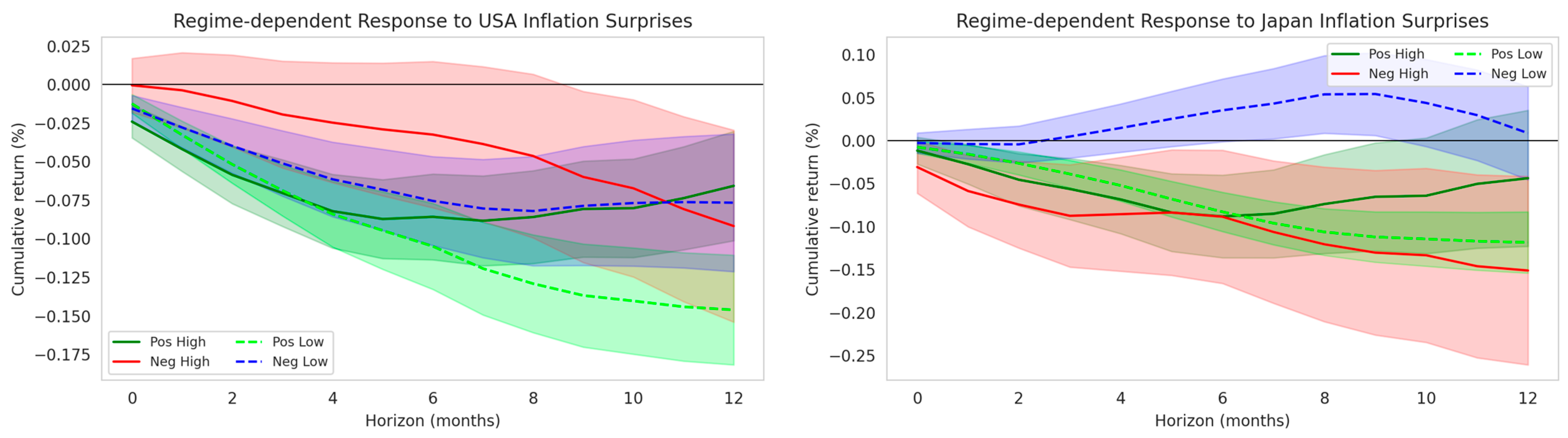
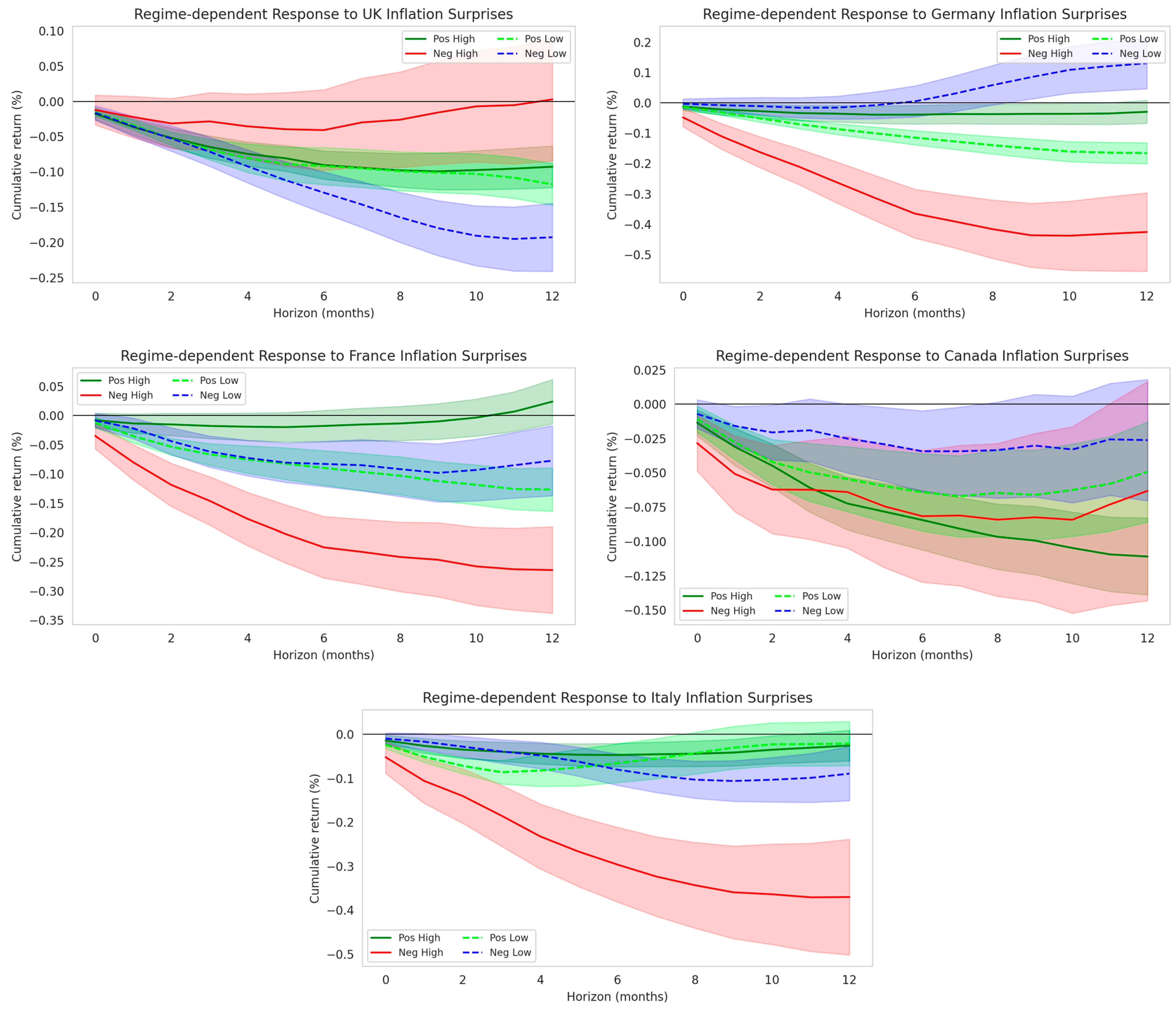
and in Figure 7, yield several stylized facts. High-negative shocks dominate, with the most significant cumulative losses observed in Germany, Italy, and France. Low-positive shocks are also damaging, particularly in the United States, Japan, Germany, and France, indicating vulnerability when inflation is below the median but rising. By contrast, high-positive shocks are largely neutral and fade over time. The United States and France show relative insulation, while Germany and Italy remain extremely fragile. Finally, regime asymmetry is evident: some markets, such as Germany and Japan, exhibit sign reversals across regimes, underscoring the interaction between the inflation state and shock direction.

The country-by-country analysis reveals that the United States shows consistent losses across regimes, but the magnitude varies. At the one-year horizon, low-positive shocks lead to the largest decline (−14.6%), while high-regime shocks are smaller (−6.6% to −9.2%). This defies the usual expectation that high-inflation states amplify equity sensitivity. The pattern is consistent with U.S. markets being more vulnerable when inflation is below the median, and positive surprises undermine expectations of stability. On the other hand, once inflation is already high, the credibility of monetary policy and inflation anchoring appear to mitigate the downside further (Campbell & Vuolteenaho, 2004; Clarida et al., 2000; Bernanke & Kuttner, 2005).

Japan displays a strong asymmetry. Negative shocks under low inflation dissipate and even turn slightly positive (+0.9% at one year), while low-positive shocks are costly (−11.8%). High-inflation regimes reverse this pattern: both positive and negative shocks depress valuations, with particularly severe negative shocks (−15.1%). These results could reflect Japan’s historical sensitivity to deflationary risks under low inflation and to credibility concerns under high inflation. When inflation is low, positive shocks trigger sharp adjustments in real rates and expectations of tightening, reducing valuations. Under high inflation, both directions undermine investor confidence, reflecting the vulnerability of Japanese firms’ cash flows to real-rate volatility and external demand shocks. The UK market is most vulnerable to low-negative shocks (−19.3% at one year). Other shocks, including high-regime disturbances, are more muted. This asymmetry implies that deflationary surprises under subdued inflation undermine expectations, triggering higher premia for external financing. The UK illustrates the risk-premium channel, in which global investors respond strongly to signs of weak domestic demand and limited policy space (Bartram & Bodnar, 2009; Connolly et al., 2005).

Germany exhibits striking sign and regime dependence. Low-negative shocks become positive (+13.0%) after one year, while low-positive shocks yield declines (−16.6%). Under high inflation, negative shocks dominate, generating the largest drop across the G7 (−42.5%). This extreme sensitivity to high-negative surprises aligns with Germany’s export-driven model, where inflationary contractions in global demand magnify losses. France reveals a defensive profile. Positive shocks in the high regime are neutral to slightly positive (+2.4%), while negative shocks are clearly damaging (−26.4%). In the low regime, both signs generate losses, but of smaller magnitude (−7.7% to −12.7%). The resilience to upside surprises points to the stabilizing role of defensive sectors and institutional features, such as wage indexation (Blanchard & Muet, 1993). Canada shows relatively symmetric outcomes. Losses occur under all shocks, ranging from −2.6% to −11.1%. High-positive shocks are the most damaging, consistent with the commodity-intensive nature of the Canadian market, where inflationary pressures and tighter expectations reduce valuations. Italy stands out for its vulnerability to high-negative shocks (−37.0%). Other shocks are moderate (−2% to −9%). Contrary to prior claims, high-positive shocks are not catastrophic. The Italian equity market’s weakness may be associated with the sovereign debt overhang (Laeven & Valencia, 2018). In fact, inflationary contractions raise doubts about fiscal sustainability, and negative surprises elevate equity risk premia disproportionately (Corsetti & Dedola, 2016; Balduzzi et al., 2001).

In detail, many patterns emerge from these results. First, high-negative shocks produce the most profound and most consistent losses across countries, particularly in Germany, Italy, and France. Second, low-positive shocks are also damaging, especially in the United States, Japan, France, and Germany. Third, high-positive shocks are largely neutral or of limited scale in most countries, suggesting that equity markets absorb inflationary pressures once inflation is already high. Fourth, regime-dependent sign flips occur, and the same type of shock has opposite effects across regimes. Germany and Japan experience low-negative shocks that eventually reverse into gains, underscoring the importance of horizon choice.

Table 12. Summary of dominant inflation shock effects on G7 equity markets at h = 12.

Country	Most Negative Regime	Effect (h = 12)	Least Negative/ Positive Regime	Effect (h = 12)	Dominant Pattern	Key Insight
USA	Low_pos	−0.1462	High_pos	−0.0657	All regimes negative	Low inflation increases hit hardest. High inflation decreases are least damaging.
Japan	High_neg	−0.1512	Low_neg	0.0088	Mixed (positive in Low_neg)	Unique resilience: Low inflation decreases boost returns.
UK	Low_neg	−0.1929	High_neg	0.0028	Mixed (positive in High_neg)	Extreme sensitivity to low inflation decreases. High inflation decreases neutralize the harm.
Germany	High_neg	−0.4255	Low_neg	0.1302	Mixed (strong positive in Low_neg)	Most severe high inflation damage. Low inflation decreases strongly benefit.
France	High_neg	−0.2641	High_pos	0.0236	Mixed (positive in High_pos)	High inflation decreases catastrophic. High inflation increases fade or turn positive.
Canada	High_pos	−0.1109	Low_neg	−0.0263	All regimes negative	High inflation increases are most harmful. Low inflation decreases are the least damaging.
Italy	High_neg	−0.3701	Low_pos	−0.0208	All regimes negative	High inflation decreases devastate. Low inflation increases mildest.

summarizes the dominant patterns at the one-year horizon. It highlights, for each G7 market, the regime–shock combination that generates the largest cumulative losses, as well as the regime in which markets are least affected. This comparison makes it clear that high-negative shocks are the principal drivers of equity declines, while positive shocks under high inflation often fade or even turn slightly positive. The pattern is consistent with frameworks emphasizing state-dependent risk premia and the asymmetric role of negative macroeconomic news (Cogley & Sargent, 2005).

The country-specific patterns documented above point to meaningful heterogeneity in how inflation shocks transmit to equity markets. While institutional and structural factors offer plausible explanations for these differences, our empirical framework identifies conditional responses rather than causal mechanisms. We explore these interpretive channels more systematically in the next section.

6. Interpreting Cross-Country Heterogeneity

Our preceding analysis reveals pronounced conditional differences in how G7 equity markets respond to inflation shocks across regimes and shock directions. While Italy shows acute conditional vulnerability in low-inflation environments, Japan displays relative conditional resilience, and the United States and France appear more insulated. These patterns are not merely statistical artifacts; they likely reflect deeper structural and institutional differences that shape how inflation risk is transmitted to financial markets. It is important to clarify that our empirical design identifies conditional responses—how equity returns react to inflation surprises under different regimes—rather than causal mechanisms. In this interpretive discussion, we structure several observable macroeconomic features that may plausibly explain the documented variations in responses, grounding our interpretation in established theoretical channels and the existing literature. Formal testing of these channels would require a different research framework, such as interactions between inflation shocks and time-varying country-level institutional or structural proxies, which we highlight as a valuable avenue for future study.

The credibility of monetary policy and the degree to which inflation expectations are anchored vary meaningfully across the G7. Countries with a long track record of price stability and transparent central bank communication—such as the United States and Germany—tend to exhibit more muted equity reactions to inflation surprises. When expectations are well-anchored, markets may perceive inflationary spikes as temporary, limiting the repricing of long-term discount rates. In contrast, economies where inflation expectations have historically been less firmly anchored—such as Italy, especially prior to Eurozone membership—may experience stronger and more persistent equity losses, as surprises are more likely to trigger fears of a de-anchoring spiral or aggressive monetary tightening. This channel aligns with the broader literature on central bank credibility and its role in attenuating financial market volatility (Gürkaynak et al., 2005; Bernanke & Kuttner, 2005).

Beyond monetary credibility, the industrial and sectoral makeup of national equity indices mediates the transmission of inflation shocks. Export-oriented economies with large manufacturing sectors—notably Germany and Japan—are sensitive to global demand and exchange-rate movements that often accompany inflation surprises. For Germany, negative inflation shocks in high-inflation regimes may signal weakening external demand, compounding equity losses. Conversely, economies with a higher share of defensive or non-cyclical sectors—such as France, with its substantial consumer-staples and utilities representation—may exhibit greater resilience, as cash flows in these sectors are less sensitive to cyclical inflation fluctuations. The United States’ diversified sectoral profile and deep capital markets further contribute to its ability to absorb inflation news without destabilizing repricing.

Elevated public debt levels can also amplify equity markets’ sensitivity to inflation surprises through the sovereign risk channel. In high-debt economies like Italy and Japan, inflation shocks—particularly negative ones in already-low-inflation environments—may raise concerns about debt sustainability, real growth prospects, and potential fiscal dominance. These concerns can spill over into equity risk premia, especially for domestic banks and corporations with large holdings of sovereign debt. This mechanism is consistent with the “doom loop” literature that links sovereign and corporate credit risk in financially integrated economies (Acharya et al., 2014; Corsetti & Dedola, 2016). By contrast, lower-debt economies such as Germany and Canada may face less acute fiscal risk transmission, allowing equity markets to focus more narrowly on cash flow and discount-rate effects.

The ability of policymakers to respond credibly and flexibly to inflation developments further shapes market reactions. Countries operating within constrained monetary frameworks—such as Italy within the Eurozone, where monetary policy is set supranationally—may exhibit heightened sensitivity because domestic tools to offset inflationary or disinflationary pressures are limited. Conversely, economies with independent monetary policy and ample fiscal space, like the United States, can more easily signal or implement countervailing measures, thereby containing the equity market impact of inflation surprises. The United Kingdom’s post-Brexit policy autonomy and Japan’s long experience with unconventional monetary easing represent intermediate cases where policy responsiveness itself has become a factor in market pricing.

These considerations offer an interpretation of the main cross-country findings. Italy’s vulnerability in low-inflation regimes likely reflects the interaction of high public debt, a fragile banking sector, and constrained policy space within the monetary union—conditions that could magnify the perceived downside risks of disinflationary surprises. Japan’s resilience, by contrast, may stem from its entrenched deflationary expectations, a large base of patient domestic investors, and a sectoral structure that is less exposed to cyclical inflation pressures. Germany’s export-driven sensitivity and France’s defensive profile can be traced to their differing industrial compositions and external exposures, while the United States’ broad insulation appears consistent with its deep financial markets, credible inflation-targeting regime, and flexible policy environment.

We highlight that, although grounded in observable macroeconomic features and well-established theoretical channels, these interpretations remain speculative given our empirical approach. Separating the exact causal impact of each channel would require a more detailed, identification-focused method. Such analysis is beyond this paper’s scope but offers a promising path for future research.

However, a more systematic assessment of market fragility requires moving beyond narrative interpretation. In the next section, we develop a quantitative framework—the Sensitivity–Volatility–Vulnerability (SVV) assessment—that distills the multidimensional nature of regime-dependent responses into comparable, country-level metrics.

7. Sensitivity–Volatility–Vulnerability (SVV) Analysis

Even though the regime–sign decomposition establishes clear asymmetries in how equity markets react to inflation shocks, it does not fully capture differences in the magnitude, persistence, and stability of those responses. To address this and move beyond directional effects, we introduce a complementary analysis of Sensitivity–Volatility–Vulnerability (SVV). This framework allows us to distinguish markets that merely react from those that are structurally fragile—where shocks translate into amplified volatility and prolonged drawdowns. In doing so, the SVV analysis identifies not only where losses occur but also where they become systemic, offering additional insight into policy credibility, financial resilience, and cross-country risk transmission.

The SVV framework extends the impulse response analysis in several ways. First, it is explicitly multidimensional, combining information on response magnitude, stability, and directional bias into a single diagnostic. Second, it is regime-conditional, focusing on how sensitivity and volatility change when inflation is high versus low—a question that average IRFs or unconditional volatility measures cannot answer. Third, it offers a classificatory output, grouping markets into vulnerability profiles that are more directly informative for risk-management and macroprudential policy than standalone coefficient estimates or volatility statistics.

The SVV concept builds on the financial resilience theory that defines resilience as the system’s capacity to absorb shocks without permanently losing function. Resilience reflects the manner in which institutional quality, fiscal flexibility, and market depth buffer against shocks (Haldane & May, 2011). A resilient market will exhibit limited price reactions, stable adjustments, and short-lived effects. By contrast, a fragile market amplifies shocks through leverage, debt rigidity, or weak policy credibility—manifesting as high SVV.

To quantify cross-country heterogeneity in regime-dependent reactions to inflation shocks, we construct two complementary measures. A Regime Sensitivity Score that captures the magnitude of response asymmetry across inflation regimes, and a Regime Volatility Measure that captures dispersion within regimes. The Regime Sensitivity Score is a composite statistic that summarizes how strongly a country’s equity market response differs between high- and low-inflation environments. It is computed in three steps:

For each country and shock direction (positive vs. negative), we estimate the standardized difference between high- and low-regime responses using Cohen’s d:

$$d={\displaystyle \frac{{\mu }_{high}-{\mu }_{low}}{{\sigma }_{pooled}}},$$

where ${\mu }_{high}$ is the mean response in high-inflation regime, ${\mu }_{low}$ is the mean response in the low-inflation regime, and ${\sigma }_{pooled}=\sqrt{{\displaystyle \frac{\left(n_{high}-1\right){\sigma }_{high}^2+\left(n_{low}-1\right){\sigma }_{low}^2}{n_{high}+n_{low}-2}}}$.

Then, we compute two separate effect sizes. A Negative_Effect_Size to assess regime effect for negative inflation shocks, and a Positive_Effect_Size to assess regime effect for positive inflation shocks. The overall regime sensitivity (CSS) is defined as the absolute sum of both effects:

$$Composite Sensitivity Score \left(CSS\right)=\left|d_{negative}\right|+\left|d_{positive}\right|$$

(5)

This composite measure captures the total magnitude of regime-dependent variation. Higher scores indicate stronger regime asymmetry in equity responses. The regime’s sensitivity is quantified and classified according to established thresholds. Measurements are interpreted as follows: values greater than 3.0 indicate high sensitivity, values between 1.5 and 3.0 indicate moderate sensitivity, and values below 1.5 indicate low or negligible sensitivity.

In addition, to capture the dispersion of equity responses within regimes, we construct a simple composite volatility metric that aggregates variation across shock types. For each country and regime, we compute the standard deviation of negative inflation shock responses ${\sigma }_{neg}$, and the standard deviation of positive inflation shock responses ${\sigma }_{pos}$. Finally, we derive a single volatility index per regime: ${Volatility}_{regime}=\sqrt{{\displaystyle \frac{{\sigma }_{neg}^2+{\sigma }_{pos}^2}{2}}}$.

This captures the total dispersion of responses irrespective of the shock sign. Relative volatility or the regime volatility difference is measured as:

$$∆Volatility={Volatility}_{high}-{Volatility}_{low}$$

(6)

Positive values indicate volatility amplification under high inflation, while negative values imply stabilization. Higher values indicate greater dispersion in market reactions. Regime differences exceeding 0.01 are interpreted as economically meaningful shifts in volatility.

The analysis in

Table 13. Comparative sensitivity and volatility metrics across G7 countries.

Country	Sensitivity Score	Cohens d Negative	Cohens d Positive	Low Regime Volatility	High Regime Volatility	Volatility Difference	Negative Effect Size *	Positive Effect Size *
USA	1.67	0.912	0.759	0.035	0.025	−0.011	Large	Medium to large
Japan	4.62	−4.173	0.445	0.033	0.030	−0.003	Very large	Small to medium
UK	2.33	2.166	0.168	0.050	0.021	−0.028	Very large	Small
Germany	5.29	−3.308	1.984	0.054	0.097	0.042	Very large	Very large
France	4.99	−2.153	2.834	0.032	0.054	0.022	Very large	Very large
Canada	4.34	−3.352	−0.989	0.013	0.025	0.012	Very large	Large
Italy	3.11	−2.384	0.722	0.030	0.078	0.048	Very large	Medium to large

(*): Effect sizes follow standard conventions with absolute values (small: 0.2, medium: 0.5, large: 0.8).

shows significant differences between countries. Markets in Japan (4.62), Germany (5.29), France (4.99), Canada (4.34), and Italy (3.11) are highly sensitive to changes in inflation. These countries exhibit large effect sizes and, in some cases, economically meaningful shifts in volatility. Germany is the most sensitive, combining large asymmetric responses with substantial volatility increases.

Japan exhibits asymmetric sensitivity with a Cohen’s d of −4.17 for negative shocks—the largest magnitude observed across all countries—and at the same time shows relatively modest sensitivity to positive shocks (d = 0.44). This 9.4:1 asymmetry ratio indicates that Japanese inflation responds disproportionately to deflationary pressures in high regimes, which is consistent with the country’s historical experience with persistent deflationary episodes and the challenges of escaping liquidity traps. Notably, Japan maintains relatively stable volatility across regimes (−0.003), suggesting that, while the magnitude of responses varies dramatically by shock direction, overall predictability remains consistent.

France and Canada display strong bidirectional sensitivities. Nevertheless, France shows a large positive shock effect. In Italy, sensitivity is driven primarily by negative shocks that are associated with regime-dependent increases in volatility. By contrast, the United States and the United Kingdom fall into the moderate sensitivity range. Both exhibit more stable cross-regime behavior and a volatility that declines in high-inflation states, suggesting greater resilience. These results confirm that vulnerability to inflation shocks is not uniform across the G7 and is reinforced when high sensitivity coincides with volatility escalation.

Furthermore, we can observe the prevalence of asymmetric responses to positive versus negative shocks. Five of seven countries exhibit strong asymmetric patterns, with negative shocks dominating. The UK shows the most extreme asymmetry (12.9:1 ratio), followed by Japan (9.4:1) and Canada (3.4:1). This systematic bias toward negative shock sensitivity suggests that deflationary pressures may be more readily transmitted across regime changes than inflationary pressures.

The analysis of the combined behavior of sensitivity and volatility provides insights into the sources of market fragility. Markets like Germany, France, Japan, and Italy, where regime sensitivity is high and volatility amplifies under inflation stress, appear more exposed to credibility risks and structural constraints. On the other hand, the United States and the United Kingdom exhibit moderate sensitivity and volatility compression in high-inflation regimes, suggesting stronger monetary credibility and greater capacity to absorb shocks without destabilizing price dynamics. These findings show that what matters for vulnerability is not only the magnitude of the shock but also institutional resilience and market structure. Countries that face significant fiscal pressures or are highly dependent on exports, particularly commodity exports, may exhibit clearer signs of regime fragility. As a result, inflation shocks in these markets are more likely to propagate into broader financial instability, reinforcing the importance of policy coordination and forward guidance in periods of inflation uncertainty.

Table 14. G7 Sensitivity–Volatility–Vulnerability profiles.

Country	Sensitivity Level	Volatility Pattern	Vulnerability Category	Key Insight
USA	Moderate	Volatility decreases in high regime	Resilient	Stable responses, limited fragility
UK	Moderate	Volatility reductions	Resilient	Sensitive to low-neg shocks, otherwise stable
Japan	High	Small volatility change	Fragile	Extreme negative shock sensitivity
Germany	High	Volatility increases strongly	Fragile	Most sensitive, highest vulnerability
France	High	Volatility increases	Fragile	Large effects in both directions
Canada	High	Volatility increases	Fragile	Regime-dependent fragility, commodity exposure
Italy	High	Volatility increases strongly	Fragile	Negative shocks drive persistent vulnerability

summarizes the G7 Sensitivity–Volatility–Vulnerability profiles.

To go further, we extended the analysis and developed a composite vulnerability assessment that integrates sensitivity, volatility amplification, and response asymmetry into a unified metric. The measure provides a structural evaluation of inflation-induced fragility across the G7 countries. The Composite Vulnerability Score (CVS) employs a weighted aggregation methodology and is calculated as follows:

$$CVS=0.5\times {Sensitivity}_{Norm}+0.3\times {Volatility}_{Norm}+0.2\times {Asymmetry}_{Norm}$$

(7)

It integrates three complementary dimensions of regime-dependent market reactions. Each component is constructed as follows.

$${Sensitivity}_{Norm}=Min\left({\displaystyle \frac{CSS}{6.0}},1.0\right)\times 100$$

(8)

$${Volatility}_{Norm}=Min\left({\displaystyle \frac{\left|∆Volatility\right|}{0.05}},1.0\right)\times 100$$

(9)

$${Asymmetry}_{Norm}=Min\left({\displaystyle \frac{Asymmetry Ratio}{15.0}},1.0\right)\times 100$$

(10)

$$Asymmetry Ratio={\displaystyle \frac{Max\left(\left|d_{negative}\right|,\left|d_{positive}\right|\right)}{Min\left(\left|d_{negative}\right|,\left|d_{positive}\right|\right)}}$$

(11)

The different components of this measure are normalized to a 0–100 scale. The magnitude of differential responses across inflation regimes is measured by the sensitivity component identified in Equation (5), normalized by the maximum observed sensitivity (6.0), and we use the previously calculated scores. The absolute change in market volatility between low- and high-inflation regimes (Equation (6)) is measured by the volatility component normalized by the maximum observed volatility shift (0.05). The asymmetry component measures the ratio of maximum to minimum Cohen’s d effect sizes for positive and negative shocks, normalized by the maximum observed asymmetry ratio (15.0). Based on our calculations, the countries are classified into four vulnerability categories: critical (CVS ≥ 70), high (50 ≤ CVS < 70), moderate (30 ≤ CVS < 50), and low (CVS < 30).

The Composite Vulnerability Score is constructed using a weighting scheme of 0.5, 0.3, and 0.2, that reflects the hierarchical contribution of each component to regime-dependent inflation risk. Because it captures the fundamental magnitude of market responses across inflation regimes, sensitivity receives the largest weight (0.5). It represents the core transmission channel through which regime shifts translate into changes in equity valuation and is therefore the most direct indicator of vulnerability severity.

Volatility is assigned a moderate weight (0.3) as it reflects the stability and predictability of market reactions under different inflation conditions. Volatility shifts do not drive vulnerability on their own, but they amplify or dampen the impact of sensitivity. In detail, they influence the persistence and the uncertainty of regime effects. This component measures the degree to which inflation shocks generate destabilizing uncertainty, a secondary but critical dimension of regime fragility.

Asymmetry receives a lower weight (0.2) because it captures directional imbalances—whether markets react more strongly to inflationary or deflationary shocks—rather than overall magnitude. Asymmetry provides important qualitative insight into the character of vulnerability, especially in economies exposed to deflation risk, but it does not fundamentally alter the scale of regime effects. The lower weight prevents extreme directional biases from dominating the composite index while ensuring their influence is incorporated.

The weighting scheme (0.5, 0.3, 0.2) reflects our assessment of the relative importance of each dimension in capturing regime-dependent vulnerability. However, alternative choices would alter the composite scores and could affect the ordinal ranking of countries near classification boundaries. The resulting Composite Vulnerability Score should therefore be interpreted as a heuristic, comparative tool rather than a precise cardinal measure of structural fragility. Its value lies in synthesizing multidimensional information into a single diagnostic for cross-country comparison, not in the exact numerical values or rankings themselves.

Moreover, we tested the robustness of the composite scores to alternative specifications. Equal weighting (33.3–33.3–33.3) and alternative hierarchies (40–40–20; 60–25–15) produced largely stable ordinal rankings and vulnerability classifications. Even under extreme weighting (70–20–10), which emphasizes sensitivity almost exclusively, the identification of the most vulnerable and most resilient economies remained unchanged. These checks suggest that while the exact numerical scores are sensitive to weighting choices, the broad comparative patterns are robust.

Our calculations in

Table 15. Composite vulnerability framework for G7 equity markets.

Country	Vulnerability Score	Vulnerability Level	Sensitivity Score	Volatility Impact	Asymmetry Ratio
Germany	71.79	Critical	5.29	0.0424	1.67
Italy	58.82	High	3.11	0.0476	3.30
France	56.50	High	4.99	0.0220	1.32
UK	53.76	High	2.33	−0.0285	12.91
Japan	52.83	High	4.62	−0.0031	9.38
Canada	47.63	Moderate	4.34	0.0116	3.39
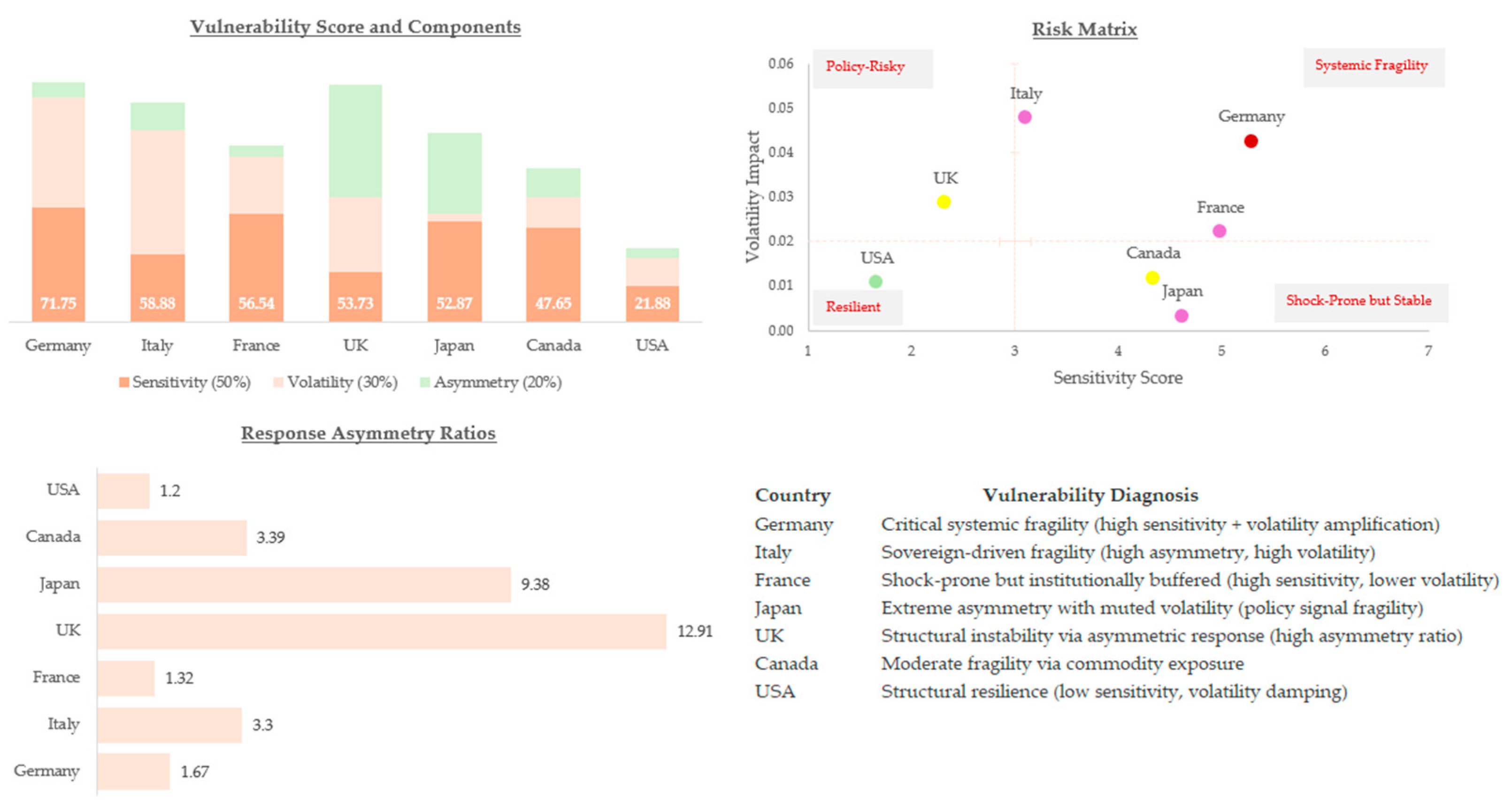
USA	21.86	Low	1.67	−0.0106	1.20

reveal a clear distinction in inflation regime risk across the G7 economies. Germany emerges as the sole critical-risk economy (CVS = 71.8). This reflects, for this country, an exceptional combination of the highest sensitivity score (5.29), substantial volatility increases (0.042), and moderate asymmetric responses (1.67:1 ratio). A group of highly exposed countries includes Italy (58.8), France (56.5), the United Kingdom (53.8), and Japan (52.8). Italy’s fragility arises from its largest observed volatility impact and its high asymmetry, which may imply a deterioration in predictability during high-inflation periods. France demonstrates high sensitivity but manageable volatility changes, while the UK and Japan’s vulnerabilities arise from extreme asymmetry—12.9:1 and 9.4:1, respectively—underscoring their exposure to one-sided market reactions. Canada falls into the moderate vulnerability category (47.6), while the United States remains the only low-vulnerability economy (21.9), exhibiting stability across all dimensions.

It is also important to mention that the geographic distribution of vulnerability reveals a pronounced regional concentration. Continental European economies—Germany, France, and Italy—as shown in Figure 8, form a contiguous high-vulnerability zone. This clustering suggests common structural features, such as fiscal rigidities, banking system exposures, and reliance on external demand, that intensify the transmission of inflation shocks under different regimes. The concentration of fragility in the euro area increases the risk of synchronized market reactions to inflation surprises, especially due to the constraints of a shared monetary framework that limits individual policy responses. In such an environment, inflation shocks may propagate not only within domestic markets but also across borders, amplifying systemic exposure at the regional level. In contrast, the North American economies—Canada and the United States—form a distinct low-to-moderate vulnerability bloc that may be characterized by a stronger policy credibility and a more flexible financial structure. Unlike the European case, vulnerability in North America does not stem from systemic fragility but from cyclical transmission. This implies a lower risk of region-wide destabilization following inflation surprises. A third regional pattern emerges in Japan and the United Kingdom, which exhibits hybrid vulnerability driven primarily by asymmetric market responses rather than volatility amplification. Both economies show high sensitivity to inflation regime shifts but retain relative stability in volatility, indicating that fragility is conditional rather than systemic. In the UK, vulnerability is concentrated in extreme negative shock asymmetry, which may reflect concerns about demand weakness and policy uncertainty. Japan’s profile shows a persistent deflationary bias, where negative surprises lead to larger equity losses. Unlike continental Europe, where vulnerability is rooted in structural instability, or North America, where resilience dominates, Japan and the UK occupy an intermediate position in which market fragility is activated only under specific shock directions or policy signals.

These three regional profiles—systemic vulnerability in continental Europe, conditional fragility in Japan and the United Kingdom, and structural resilience in North America—demonstrate that the equity market consequences of inflation are fundamentally mediated by regional institutional structures rather than by inflation shocks alone.

8. Synthesis and Overall Discussion of Results

Our multidimensional analysis reveals that the G7 equity markets do not respond uniformly to inflation shocks, nor do they tell seven distinct stories. Instead, the results can be grouped into three vulnerability clusters, distinguished by the magnitude, stability, and conditional nature of equity responses. This typology, emerging directly from the integration of regime dependence, sign asymmetry, and the SVV assessment, provides a more powerful and policy-relevant synthesis than a country-by-country recounting of the results.

The first group is characterized by systemic vulnerability, in which inflation shocks trigger amplified, destabilizing reactions. Equity markets in this group, principally Germany and Italy, exhibit high sensitivity to regime shifts and a pronounced increase in return volatility during periods of high inflation. Their responses are not only large but also become less predictable under stress, as evidenced by significant losses from both positive and negative shocks when inflation is already elevated. This pattern suggests a structural fragility, in which underlying institutional or financial rigidities—such as Germany’s export-dependent industrial model or Italy’s high sovereign debt overhang—are exposed by inflation surprises, thereby propagating risk across the financial system.

A second, distinct pattern is conditional vulnerability, in which market fragility is highly asymmetric and contingent on the direction of the shock. Japan and the United Kingdom epitomize this archetype. While demonstrating high sensitivity, these markets do not exhibit systematic volatility amplification; their defining feature is an extreme asymmetry in response. For the UK, the most severe damage arises from negative inflation surprises in low-inflation regimes, while Japan is disproportionately punished by negative shocks when inflation is high. This indicates that fragility is “switched on” by specific conditions—secular stagnation fears in the UK, or deflationary relapse anxieties in Japan—rather than representing a broad-based breakdown in market functioning.

The third archetype is characterized by structural resilience, in which equity markets absorb inflation shocks through damped, stable adjustments. The United States is the paradigmatic case, showing low-to-moderate sensitivity and volatility compression in high-inflation states. France, though following a different mechanism, also displays resilient outcomes, with consistently muted cumulative losses across specifications. This resilience likely stems from strong institutional anchors, such as the U.S. central bank’s credibility and deep capital markets, or from structural features that insulate, such as France’s large defensive sector. These economies exhibit a capacity to process inflation news without triggering destabilizing feedback loops. Canada occupies an intermediate position, displaying the commodity-driven sensitivity associated with conditional vulnerability but with less extreme asymmetry and moderate overall vulnerability scores.

This tripartite framework—systemic, conditional, resilient—integrates our discrete empirical findings into a coherent picture of cross-country financial resilience. It moves the discussion beyond confirming the average negative effect of inflation on equities, offering instead a diagnostic for how and under what conditions inflation shocks translate into financial stress. Such a synthesis provides clearer guidance for differentiated risk management and better macroprudential policy.

Our findings carry direct implications for monetary authorities and financial regulators, though we emphasize that these implications derive from observed conditional responses rather than causal tests of policy mechanisms. The documented heterogeneity in vulnerability profiles suggests that a uniform approach to inflation risk management may be inadequate.

First, the results underscore the potential value of monetary policy credibility for financial stability. Markets with historically well-anchored inflation expectations (e.g., the United States and Germany) exhibit more stable, muted equity reactions to inflation surprises, consistent with the view that central bank credibility can buffer against nonlinear financial repricing. This observation suggests that preserving credibility is not only a macroeconomic objective but also a tool for financial stability—particularly when inflation approaches or exceeds target levels.

Second, the convexity of equity losses in high-inflation regimes highlights a potential cost of allowing inflation to drift persistently above target. Inflation-targeting frameworks that tolerate temporary overshoots may inadvertently increase financial fragility, as subsequent positive surprises can trigger disproportionately large valuation adjustments. While our design does not test causal policy effects, the observed pattern suggests that central banks in inflation-sensitive economies (such as Italy and the United Kingdom) might benefit from more preemptive responses to emerging inflationary pressures.

Third, differences in vulnerability call for differentiated macroprudential approaches. Systemically vulnerable markets (Germany, Italy) could warrant stricter stress-testing scenarios that account for regime-dependent amplification, while more resilient economies (United States, France) might focus on monitoring cross-border spillovers. For currency unions like the Eurozone, where monetary policy is uniform but financial vulnerabilities are not, coordinated fiscal-prudential measures may be necessary to mitigate region-wide instability.

For investors, our findings indicate that inflation risk in equities is neither linear nor uniform, requiring adjustments to traditional portfolio management practices. These implications follow from the empirical regularities we document, though implementing them would require additional validation in specific portfolio-construction frameworks. First, regime-aware asset allocation becomes crucial: the same inflation hedge may be ineffective—or even counterproductive—depending on whether inflation is low or high. In high-inflation environments, reducing exposure to equities in systemically vulnerable markets (Italy, Germany) and increasing allocations to inflation-resilient sectors or economies (U.S. defensive sectors, French equities) could mitigate downside risk, based on the patterns we observe.

Second, standard linear factor models likely understate downside inflation exposure, particularly in high-inflation regimes. Portfolio stress tests should incorporate regime-dependent equity betas, especially for international allocations. Third, cross-country diversification benefits are conditional: while spreading investments across G7 economies reduces idiosyncratic risk, it does not eliminate inflation risk, because vulnerability profiles differ sharply. A blend of structurally resilient (U.S.) and conditionally vulnerable (Japan, U.K.) markets may offer a better inflation-adjusted risk-return profile than a pooled G7 portfolio.

In summary, recognizing the nonlinear, regime-dependent, and country-specific nature of inflation risk allows both policymakers and investors to move beyond average-case scenarios and tailor their responses to the actual state of the economy—a critical adjustment in an era where inflation volatility has returned as a central concern. These implications, while derived from conditional correlations rather than causal tests, provide a structured framework for navigating inflation risk in an increasingly complex financial landscape.

9. Conclusions and Directions for Future Research

This study has examined how inflation surprises affect real equity returns across the G7 economies, revealing that the relationship is neither uniform nor linear. By extending and integrating existing approaches within a nonlinear local projection framework, we document a double asymmetry in equity market responses. The impact of inflation shocks depends both on their direction—positive surprises are generally penalized more strongly than negative surprises are rewarded—and on the prevailing inflation regime, with high-inflation environments amplifying losses in most markets. These asymmetries point to systematic cross-country differences in how financial markets process inflation risk.

Our cross-country analysis identifies three distinct vulnerability archetypes:

• Systemically vulnerable markets (Germany, Italy), where inflation shocks trigger amplified and destabilizing responses.
• Conditionally vulnerable markets (Japan, UK), where fragility is highly asymmetric and contingent on specific shock directions, pointing to underlying concerns about deflationary risks or demand weakness.
• Structurally resilient markets (US), which exhibit dampened and stable adjustments to inflation shocks, likely due to strong monetary policy credibility and deep financial markets.

These patterns challenge the conventional wisdom that equities uniformly hedge against inflation, and they underscore the limitations of linear models and pooled cross-country analyses. Our newly developed Sensitivity–Volatility–Vulnerability (SVV) framework further highlights that financial fragility is not just about the magnitude of market reactions, but also about their stability and predictability under stress. Markets such as Germany and Italy, where sensitivity is high and volatility amplifies in high-inflation regimes, face a heightened risk of inflation-induced financial instability.

For policymakers, especially central banks and financial regulators, our findings underscore the importance of preemptive and credible inflation anchoring. Allowing inflation to drift above target not only harms price stability but also increases financial fragility, as subsequent positive surprises can trigger nonlinear market corrections. In currency unions such as the Eurozone, the multiple vulnerability profiles—with Germany and Italy on opposite ends of the resilience spectrum—calls for differentiated macroprudential tools and closer coordination between monetary and fiscal authorities to mitigate region-wide instability.

For investors and financial institutions, the results highlight the need for regime-aware and country-specific risk management. Static asset allocation models that assume uniform inflation sensitivity across advanced economies may significantly understate downside risk, particularly in systemically vulnerable markets. Portfolio diversification should account not only for average inflation betas but also for the conditional and asymmetric nature of inflation risk.

Our results open directions for further investigation. In fact, the heterogeneity across countries suggests that aggregating to the national equity index level is informative, but it also masks important underlying mechanisms. Future work could explore these channels to develop a more granular, theoretically grounded understanding.

A primary direction involves a more detailed microeconomic analysis of the national results. The contrast between countries like Italy and France begs for a sectoral decomposition. Implementing the local projections framework on industry-level equity indices could pinpoint whether the asymmetric penalties are concentrated in specific sectors—such as highly leveraged banks, energy-intensive manufacturers, or rate-sensitive growth stocks—thereby identifying the precise transmission channels of inflation news. Furthermore, the “Italian anomaly,” where low inflation and negative surprises trigger severe losses, is an interesting puzzle. An analysis that may integrate credit default swap (CDS) spreads or other sovereign credit risk proxies into a multivariate framework could disentangle whether this effect is driven primarily by a sovereign risk premium spilling into corporate discount rates or by sector-specific cash flow vulnerabilities.

Furthermore, the use of high-frequency identification techniques could offer a new approach for causal identification. Analyzing intraday data around precise CPI announcement times would allow researchers to cleanly separate the immediate, likely discount-rate-driven market reaction from the slower reassessment of long-term cash flows. Complementing this, future models could incorporate direct measures of inflation expectations from surveys or market break-evens. This would help distinguish whether the documented relation is a function of the surprise component alone or is also influenced by the level of already-entrenched expected inflation, a distinction crucial for central bank communication strategies.

Future research should examine the structural and institutional factors behind these vulnerability differences. The asymmetries observed in some markets indicate the need to move beyond symmetric models of inflation shocks and to incorporate directional transmission channels, particularly in economies with strong negative shock biases. Additionally, the geographic clustering of vulnerability observed across continental Europe highlights the need to explore cross-border spillovers and the potential for contagion within integrated monetary systems.

The vulnerability framework developed in this study may also provide a foundation for constructing early warning indicators and stress-testing tools tailored to inflation regime risk. By distinguishing between systemic, conditional, and resilient market structures, the framework implies that policy evaluation should adopt a state-contingent and a country-specific orientation rather than a uniform rules-based approach. Extending this analysis to sectoral equity indices and emerging economies would deepen our understanding of how inflation shocks propagate through heterogeneous financial architectures and, In detail, inform the design of more robust monetary and macroprudential policies. Finally, the scope of this research could be expanded in macroeconomic and theoretical dimensions. The framework could be extended to test for cross-border spillover effects to examine how a core economy’s inflation surprise transmits to foreign equities.

Answering these questions would not only deepen our understanding of the inflation–equity nexus but also equip policymakers and investors with more useful tools to navigate an era in which price stability can no longer be taken for granted.