Fiscal Regressivity and Allocative Inefficiency: The Economic Cost of Thailand’s 2024 Wine Tax Reform

Abstract

Thailand’s 2024 excise tax reform aimed to stimulate the tourism economy through the elimination of import tariffs and the reduction in excise rates on wine. This study evaluates the causal economic and distributional impacts of this policy intervention. The analysis employs a quasi-experimental Doubly Robust Difference-in-Differences (DR-DiD) estimator on a stratified cluster sample to isolate shifts in consumption expenditure, volume, and net ethanol intake. Results indicate a null effect for the general population, which confirms that the price floor remained prohibitive for median earners despite the tax reduction. The top income quintile conversely exhibited a statistically significant “additive premiumization” effect characterized by a surge in wine quantity without the substitution of other beverage categories. This behavioral shift generated a substantial Net Economic Loss driven by the divergence between foregone tax revenue and projected human capital productivity losses. The policy consequently functioned as a regressive fiscal transfer to the elite and created severe allocative inefficiency. These findings suggest that ad valorem tax incentives for luxury goods in emerging markets generate deadweight loss. Future policy strategies should therefore prioritize specific volumetric taxation to align fiscal incentives with public health objectives.

1. Introduction

Alcohol consumption constitutes a complex dietary behavior with profound implications for public health nutrition and chronic disease epidemiology. Beyond its psychotropic effects, ethanol acts as a non-essential, energy-dense nutrient that directly contributes to the etiology of diet-related disorders, including metabolic syndrome, liver disease, and cardiovascular pathology (Rehm et al., 2010a; World Health Organization, 2018). In Southeast Asia, the nutritional landscape has shifted dramatically over the past three decades. Rapid economic development has coincided with a “nutrition transition” characterized by increased consumption of processed commodities and exposure to lifestyle risk factors (Kosulwat, 2002). Thailand presents a critical case study of this transition, where the burden of alcohol-attributable morbidity has escalated to crisis levels.

Official surveillance data from the Thai Ministry of Public Health reveals a rapid deterioration in non-communicable disease (NCD) prevalence over the last 17 years. Between 2007 and 2024, the inpatient hospitalization rate for hypertension (ICD-10: I10–I15) surged from 1025.4 to 3205.4 per 100,000 population. This represents a 3.1-fold increase in less than two decades (Ministry of Public Health, 2024). Concurrently, hospitalization rates for stroke (I60–I69) nearly tripled, rising from 255.8 to 743.1 per 100,000 population over the same period (Ministry of Public Health, 2024). This epidemiological data indicates a population increasingly vulnerable to metabolic stressors, for which excessive ethanol intake is a potent aggravator.

Despite this growing burden of diet-related chronic disease, fiscal policy regarding alcohol has often prioritized economic stimulation over public health protection. On 23 February 2024, the Thai government implemented a sweeping reduction in excise taxes and import tariffs for wine. Crucially, this fiscal restructuring was an autonomous domestic policy decision designed to stimulate the tourism and leisure economy rather than a compliance measure mandated by international trade agreements. The reform created a mixed incentive structure, detailing a reduction in the ad valorem excise rate from 10% to 5% for premium tiers and the complete elimination of import tariffs, as detailed in

Table 1. Comparison of tax structure for wine before and after 23 February 2024.

Tax Component	Product Category	Pre-Reform	Post-Reform
Import Tariff (on CIF value)	Grape & Fruit Wine	54–60%	0%
Excise Tax (ad rem) (THB per liter of pure alcohol)	Grape Wine	1500	1000
	Fruit Wine	900	900
Excise Tax (ad valorem)	Grape Wine (Price < 1000 THB)	0%	5%
	Grape Wine (Price ≥ 1000 THB)	10%	5%
	Fruit Wine (Price < 1000 THB)	0%	0%
	Fruit Wine (Price ≥ 1000 THB)	10%	0%

Source: Thailand’s Ministry of Finance.

(The Secretariat of the Cabinet, 2024). Official government projections indicated that this liberalization, while intended to boost tourism, would result in a combined annual revenue loss of approximately 579 million THB.

A robust body of evidence confirms that excise taxes are typically cost-efficient instruments for reducing aggregate consumption and associated harms (Chaloupka et al., 2019; Elder et al., 2010; World Health Organization, 2017). Standard economic theory and meta-analyses consistently demonstrate that demand is responsive to price changes (Gallet, 2007; Wagenaar et al., 2009). However, the public health implications of a tax reduction depend heavily on how consumers adjust the nutritional quality and composition of their consumption basket.

From a health economics perspective, the critical variable is not consumer spending, but net ethanol intake. If a tax cut induces consumers to substitute lower-ABV beverages, such as Beer at approximately 5%, for higher-ABV beverages, such as wine at approximately 12.5%, the policy may inadvertently increase the population’s toxicological exposure to alcohol. We term this phenomenon “ethanol-driven premiumization,” where the total liquid volume consumed may remain constant while the ethanol load increases (Gruenewald et al., 2006). This risk is particularly acute in regions already struggling with high mortality from metabolic conditions. For instance, Thailand’s Southern region, which has experienced the fastest acceleration in stroke mortality since 1998, represents a demographic highly susceptible to policy-induced health shocks (Ministry of Public Health, 2024).

The primary objective of this study is to evaluate the causal economic and distributional impacts of Thailand’s 2024 wine tax reform. Specifically, we investigate whether the ad valorem tax reduction successfully stimulated aggregate demand or merely generated a windfall for high-income consumers. Based on the theory of positional goods and premiumization, we test two core hypotheses. First, the Null Effect Hypothesis (H1) posits that for the general population (low-to-middle income), the tax reduction will yield no significant change in wine consumption due to prohibitive baseline prices. Second, the Additive Premiumization Hypothesis (H2) posits that high-income consumers will respond to the tax cut by increasing the quantity of wine consumed (an income effect) rather than substituting away from other beverages. In order to test these hypotheses, we utilize a quasi-experimental Doubly Robust Difference-in-Differences (DR-DiD) design to isolate the causal effect of the 2024 tax reform on ethanol consumption behaviors. Unlike previous evaluations that focus on tax revenue or aggregate demand elasticity (Nelson, 2013), we explicitly link behavioral shifts to the nutrient profile of the consumption basket, specifically grams of pure ethanol. We test the hypothesis that the tax reduction disproportionately encouraged high-ABV wine consumption among affluent demographics, thereby increasing their net ethanol intake during a period of critical vulnerability for the national public health system.

2. Materials and Methods

2.1. Study Design and Participants

This study employed a quasi-experimental design utilizing a multi-stage stratified cluster sampling approach to ensure national representativeness. The study population consisted of Thai citizens aged 20 years and older residing in five key geographic regions—Bangkok and its vicinity, Central, North, Northeast, and South—utilizing a multi-stage stratified cluster sampling design. The selection process proceeded in three stages. First, provinces within each region were selected via systematic sampling with probability proportional to size (PPS) based on census population data. Second, households within the selected provinces were identified using systematic random sampling. Third, within selected households, individual respondents were recruited to satisfy strict stratification quotas based on geography (regional population proportion), demographics (age group and gender), and drinking status. This stratification ensured the sample distribution matched national demographic parameters.

Data collection was conducted via a single cross-sectional survey wave administered in January 2025. The study employed a retrospective panel design to reconstruct consumption behaviors. To mitigate measurement error, the survey instrument employed a Standardized Unit Conversion protocol. Respondents reported consumption quantities using fixed unit definitions (e.g., 1 glass of wine = 150 mL; 1 bottle = 750 mL) rather than subjective estimates. Additionally, to minimize recall bias, the instrument utilized major cultural events (e.g., Songkran Festival in April, New Year) as temporal anchors to clearly delimit the reporting windows. Participants reported their average monthly consumption for two balanced 10-month intervals:

The Pre-Policy Period: Average monthly behavior for the 10 months preceding the reform (April 2023–January 2024).

The Post-Policy Period: Average monthly behavior for the 10 months subsequent to the reform (March 2024–December 2024).

We acknowledge the potential for recall bias inherent in retrospective designs; however, the use of fixed temporal anchors and standardized unit protocols was implemented to minimize telescoping effects.

2.2. Sample Size Calculation and Stratification

We rigorously determined the required sample size using the formula for estimating population proportions (Scheaffer et al., 2012) Based on a total population of 51.22 million (Ministry of Interior, 2024) and an active alcohol consumer prevalence of roughly 31% (15.97 million) (National Statistical Office, 2021), we targeted a 99% confidence level with a margin of error of 0.05. To account for variance inflation inherent in multi-stage sampling, we applied a Design Effect (DEFF) of 1.5 (Groves et al., 2009).

$$n =\mathrm{D}\mathrm{E}\mathrm{F}\mathrm{F}\times {\displaystyle \frac{Np(1-p)}{\frac{d^2}{Z_{\propto }^2}(N-1)+p(1-p)}}$$

Based on these parameters, the initial calculated sample size (n) was 571.31. After applying the Design Effect of 1.5 to account for the multi-stage sampling variance (Groves et al., 2009), the required minimum sample size was determined to be approximately 857. Our final analytical sample consisted of 834 individuals. Although slightly below the strict 99% confidence target, this sample size substantially exceeds the requirement for a standard 95% confidence level (n = 495) and provides sufficient statistical power to detect heterogeneous treatment effects in our primary interaction models.

2.3. Measures and Data Processing

We constructed four primary outcome variables to capture different dimensions of behavioral change:

• Spending (THB/month): Total reported monthly expenditure.
• Frequency (Times/month): Reported frequency of consumption occasions.
• Quantity (mL/month): Total monthly volume consumed.
• SpendPerTime (THB/Occasion): A proxy for “premiumization,” calculated as Total Spending divided by Frequency.

To quantify the nutritional and toxicological load, beverage volumes were converted to pure ethanol mass using standard Alcohol by Volume (ABV) assumptions specific to the Thai market: Wine: 12.5% ABV; Beer: 5.0% ABV; Spirits: 40.0% ABV. The conversion formula used was ethanol (g) = volume (mL) $\times$ ABV $\times$ 0.789 (density of ethanol) (World Health Organization, 2002)

2.3.1. Data Cleaning and Harmonization

In order to ensure data accuracy, we applied a strict cleaning protocol. First, to address potential measurement errors where respondents might report consumption in both “glasses” and “bottles” for the same occasion, we adopted a “Max-Operator Strategy.” We calculated the volume for both entries and retained the maximum value as the verified consumption per occasion to prevent double-counting. Raw data values were confirmed to be in milliliters (mL); therefore, no additional unit conversion factors were applied during the final calculation.

2.3.2. Handling Missing Data and Outliers

Missing values (NA) for consumption-related questions were treated as zero consumption (non-drinkers). Observations with missing data for key covariates required for propensity score estimation (income, age, and region) were excluded. To ensure biological plausibility and prevent skewing from commercial stockpiling, we applied an exclusion criterion for extreme outliers: observations reporting wine consumption exceeding 50,000 mL per month (approximately 66 bottles) were removed from the analysis.

2.3.3. Socioeconomic Stratification

To analyze heterogeneous effects, households were categorized into five distinct income tiers based on average monthly personal income. This stratification strategy was validated against national income distribution data from the Office of the National Economic and Social Development Council (NESDC) (Office of the National Economic and Social Development Council, 2025) to ensure it captured structural discontinuities in the population. The tiers are defined as follows:

Tier 1 (<15,000 THB): This tier corresponds to the bottom 80% of the national population (Deciles 1–8), where the average personal income peaks at approximately 13,494 THB. It also encompasses the national average personal monthly income of 11,321 THB.

Tier 2 (15,000–30,000 THB), Tier 3 (30,000–50,000 THB), and Tier 4 (50,000–100,000 THB): These tiers encapsulate the upper-middle class and the mass affluent (Deciles 9 and 10). NESDC data indicates that the average income of the top decile (Decile 10) is 36,706 THB. Therefore, the typical high-income earner in Thailand falls within Tier 3 or the lower bound of Tier 4.

Tier 5 (>100,000 THB): This tier isolates ultra-elite outliers. Individuals in this category possess an income exceeding the average of the top national decile nearly three-fold.

Distinguishing these specific groups allows for the testing of threshold effects. It enables the analysis to determine whether consumption surges occur linearly with income or remain latent until reaching the specific purchasing power threshold characteristic of the ultra-elite.

2.4. Statistical Analysis

To isolate the causal effect of the tax reduction on ethanol intake, we employed the Doubly Robust Difference-in-Differences (DR-DiD) estimator proposed by Sant’Anna and Zhao (2020). We selected this estimator over the canonical Two-Way Fixed Effects (TWFE) OLS model because TWFE weights can become negative and biased in the presence of heterogeneous treatment effects across groups or time.

2.4.1. Econometric Model

The analytical dataset was restructured into a stacked panel at the person–beverage level. This allowed for a direct comparison of consumption trends between the treated beverage category (Wine) and control beverage categories (Beer, Whisky, White Spirits) over the same time horizon.

Our primary parameter of interest is the Average Treatment Effect on the Treated (ATT). The DR-DiD estimator achieves consistency by combining two distinct modeling approaches: Inverse Probability Weighting (IPW) and Outcome Regression (OR). This “double robustness” property ensures that the estimator (${\widehat{\tau }}^{dr}$) remains unbiased if either the propensity score model or the Outcome Regression model is correctly specified, though both need not be. Formally, let Y_i,b,t be the outcome for individual I and beverage n in period t. The DR-DiD estimator is defined as

$${\widehat{\tau }}^{dr}= {\displaystyle \frac{1}{N_{D=1}}}{\sum }_{i=1}^N\left[{\displaystyle \frac{D_b}{\widehat{p}}}∆Y- {\displaystyle \frac{\widehat{p}\left(X\right)\left(1-D_b\right)}{\widehat{p}\left(1-\widehat{p}\left(X\right)\right)}}∆Y-\left({\widehat{m}}_1\left(X\right)-{\widehat{m}}_0\left(X\right)\right)\right]$$

(1)

where $\widehat{p}\left(X_i\right)$ is the propensity score, ensuring covariate balance between beverage types;

• $∆Y$ is the change in outcomes (Spending, Frequency, Quantity or SpendPerTime) (${\mathrm{Y}}_{\mathrm{P}\mathrm{o}\mathrm{s}\mathrm{t}}-{\mathrm{Y}}_{\mathrm{P}\mathrm{r}\mathrm{e}})$;
• $D_b$ is the treatment indicator (D = 1 if beverage b is Wine; D = 0 otherwise).

This specification relies on the Conditional Parallel Trends Assumption, positing that, conditional on consumer characteristics, the demand trends for wine and control beverages would have evolved in parallel absent the tax reform.

2.4.2. Identification Strategy

The analytical dataset was restructured into a stacked panel at the person–beverage level. This framework allowed for a direct comparison of consumption trends between the treated beverage category (Wine) and control beverage categories (Beer, Whisky, White Spirits) within the same population over the same time horizon.

Our primary parameter of interest is the Average Treatment Effect on the Treated (ATT), which captures the differential change in wine consumption relative to the counterfactual trend of non-targeted beverages. We employed the Doubly Robust Difference-in-Differences (DR-DiD) estimator, which achieves consistency by combining Inverse Probability Weighting (IPW) and Outcome Regression (OR). This estimator remains unbiased even if one of the two specifications is misspecified (doubly robust property).

Identification Assumptions:

• Treatment Group (D = 1) corresponds to wine consumption.
• Control Group (D = 0) corresponds to non-targeted beverages (Beer, Whisky, and White Spirits).
• For exclusion criteria, we strictly excluded observations for “Local Liquor/Spirits” (Surachae) from the control pool to avoid contamination from concurrent excise tax adjustments specific to that category.
• For covariates, propensity scores for the IPW component were estimated using age, gender, and urbanicity to ensure covariate balance between beverage types.

The identification relies on the Conditional Parallel Trends Assumption, positing that, conditional on consumer characteristics, the demand trends for wine and control beverages would have evolved in parallel in the absence of the tax reform. Standard errors were computed at the unit-identifier level (person–beverage pairs) to account for the serial correlation inherent in the panel data structure.

2.4.3. Robustness and Falsification

To validate that the observed divergence was driven by the specific tax incentives for wine, we conducted falsification tests. We iteratively re-assigned the treatment status to Beer and Whisky (treating them as “pseudo-treated” units against the remaining controls). The null results for these placebo tests (p > 0.05) confirm that the structural break in consumption was unique to the wine market and not an artifact of aggregate demand shocks.

In addition, given the retrospective nature of the dataset, we tested for Common Method Bias (CMB) using Harman’s Single-Factor Test. An exploratory factor analysis containing all key variables (consumption metrics and demographics) showed that a single factor explained only 27.4% of the total variance. Since this is substantially below the 50% threshold, we conclude that common method variance does not significantly bias the results (Podsakoff et al., 2003).

2.5. Economic Impact Assessment

To estimate the aggregate implication of the tax reform, we employed a prevalence-based cost-of-illness (COI) framework utilizing the Human Capital Approach (HCA) to value productivity losses. This methodology was adapted from the national standard established by Luangsinsiri et al. (2023), which found that 96.32% of the economic cost of alcohol in Thailand comprises indirect costs, predominantly productivity losses linked to market earnings potential (Luangsinsiri et al., 2023; Pritchard & Sculpher, 2000; Rice & Cooper, 1967). Consequently, the economic burden is highly sensitive to the income level of the consumer.

The Net Economic Impact ($E_{net}$) is defined as the sum of direct fiscal losses and the marginal increase in social externalities, calculated as follows:

$$E_{net}= C_{fiscal}+ C_{social}$$

where $C_{fiscal}$ represents the direct revenue loss from the reduction in excise tax rates and elimination of import tariffs, based on Ministry of Finance projections. $C_{social}$ represents the projected marginal social cost attributable to the policy-induced consumption surge.

The social cost $C_{social}$ was estimated specifically for the affected demographic identified by the DR-DiD analysis (Tier 5 consumers) using the following specification:

$$C_{social}= N_{target}\times C_{baseline}\times M_{income}\times {\Delta }_{risk}$$

Parameters were parameterized as follows:

Target Population $(N_{target})$ is the number of active drinkers in the affected high-income tier, derived by applying the tier’s prevalence rate from our survey data (2.64%) to the national active drinker population.

Baseline Economic Cost ($C_{baseline}$) is the average per capita economic cost of alcohol consumption in Thailand. This was derived from the total national cost of 165,450.45 million THB reported by Luangsinsiri et al. (2023) divided by the total active drinker population (Luangsinsiri et al., 2023; National Statistical Office, 2021).

Income Valuation Multiplier ($M_{income}$) is a multiplier derived from the ratio of the Tier 5 income threshold (100,000 THB) to the national average monthly income of 10,313.09 THB (National Statistical Office, 2022).

Marginal Risk Factor (${\Delta }_{risk}$) is the percentage increase in ethanol intake relative to the national baseline, derived directly from the quantity estimates (ΔVol) of the DR-DiD estimator.

3. Results

This section presents the empirical findings on the impact of the 2024 wine tax reduction on ethanol consumption behaviors. We first examine the baseline demographic and consumption characteristics of the sample. Second, we present causal estimates from the Doubly Robust Difference-in-Differences (DR-DiD) models, specifically analyzing heterogeneity across five distinct income tiers to test for non-linear policy responses. Finally, we report results from falsification tests to validate the identification strategy.

3.1. Descriptive Statistics and Consumption Patterns

The baseline characteristics of the analytical sample across 1641 observations (

Table 2. Baseline descriptive statistics by beverage type.

Variable	Wine	Beer	Whisky	White Spirits
N	494	589	265	143
Variables
Spending (THB)	1139.68 (1559.09)	1103.14 (1336.89)	1367.92 (1660.74)	481.82 (551.01)
Frequency (times/mo)	1.91 (2.21)	3.47 (2.89)	2.43 (2.52)	2.59 (2.63)
Quantity (mL/mo)	1552.49 (2590.77)	5448.36 (7360.44)	608.77 (955.37)	620.80 (986.17)
Ethanol intake (g/mo)	153.11 (255.51)	214.98 (290.86)	192.13 (301.51)	195.93 (311.24)
Demographics
Gender
Female	53.64%	43.63%	35.85%	17.48%
Male	46.36%	56.37%	64.15%	82.52%
Urbanicity
Urban	68.22%	66.04%	70.94%	53.15%
Rural	31.78%	33.96%	29.06%	46.85%
Regions
Bangkok	17.20%	15.10%	16.98%	13.28%
North	20.65%	17.83%	21.51%	22.38%
Northeast	33.40%	34.30%	32.45%	44.06%
South	13.16%	13.75%	9.44%	6.29%
Central	15.59%	19.02%	19.62%	13.99%

Note: Values represent means with standard deviations reported in parentheses and percentages for categorical variables. N represents unique individuals. Columns do not sum to the total sample size due to overlapping consumption of multiple beverage types by the same individuals. Source: Authors’ calculation.

) were stratified by beverage preference. The data reveal a pronounced socioeconomic gradient in alcohol consumption patterns. Wine consumers (N = 494) represent a distinct demographic profile characterized by high socioeconomic status: they are predominantly female (53.64%), reside in urban areas (68.22%), and report significantly higher average monthly incomes compared to other groups. In contrast, consumers of White Spirits (N = 143) and Local Liquor (N = 150) are predominantly male (82.52% and 64.67%, respectively) and have higher representation in rural areas. Notably, while Beer remains the most frequently consumed beverage (3.47 times/month), wine consumption is characterized by high variance in expenditure (SD = 1559.09 THB), suggesting a market divided between occasional drinkers and high-value consumers.

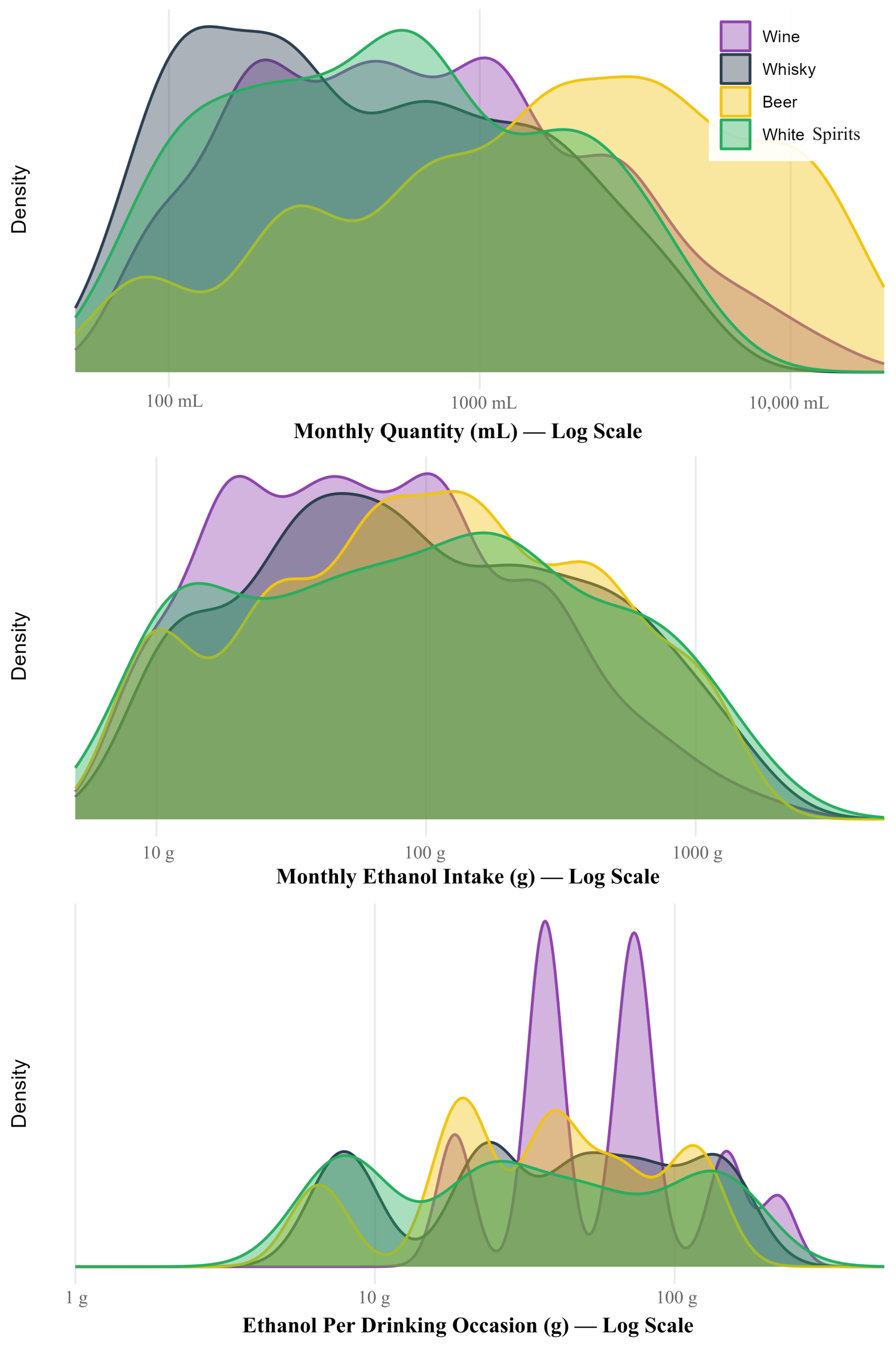
Analysis of the distribution of alcohol consumption was conducted across three metrics: monthly fluid volume (Top Panel), total monthly ethanol intake (Middle Panel), and ethanol intensity per drinking occasion (Bottom Panel) (Figure 1). First, the distribution of fluid volume (Top Panel) illustrates a distinct structural divide. Beer consumers consistently exhibit the highest fluid intake, with the density curve shifted significantly to the right (>1000 mL/month). This reflects the lower alcohol concentration and larger serving sizes typical of this category. In contrast, Spirits, including both Premium Whisky and White Spirits, are clustered at the lower end of the volume spectrum.

However, when adjusted for alcohol content (Middle Panel), the disparity in consumption volume disappears and reveals a convergence in chronic health risks. Despite the lower fluid volume, the distribution of total monthly ethanol intake for White Spirits shifts rightward to overlap significantly with that of Beer and Premium Whisky. This indicates that low-cost White Spirits facilitate a “high-ethanol, low-volume” consumption pattern, which allows consumers to achieve high chronic alcohol loads comparable to those of premium beverage consumers. The analysis of drinking intensity per occasion (Bottom Panel) further differentiates the health risks. Wine (purple) exhibits a more centralized distribution, which suggests a pattern of moderate consumption per sitting. Conversely, the distributions for Spirits, specifically Whisky and White Spirits, are notably right-skewed, with long tails extending beyond 40 to 60 g of ethanol per occasion. This pattern is indicative of higher-intensity consumption or “binge” behavior and poses elevated risks of acute toxicity despite the smaller physical volumes consumed.

3.2. Main Causal Estimates: The Socioeconomic Threshold of Consumption

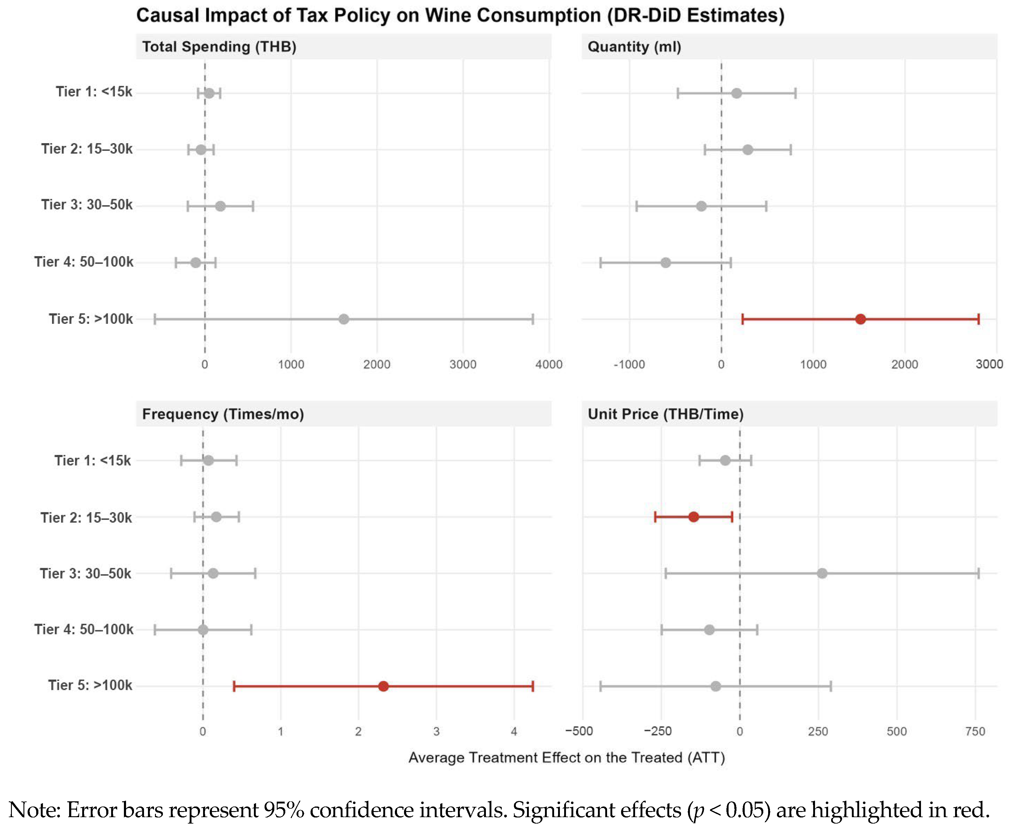
Average Treatment Effect on the Treated (ATT) derived from the DR-DiD estimator was stratified by five income tiers. The results indicate that the tax reduction did not stimulate a generalized increase in wine consumption. For the bottom four income tiers (Tier 1 through Tier 4, earning <100,000 THB/month), we observe no statistically significant changes in Spending, Frequency, or Quantity. The point estimates for these groups hover near zero, suggesting that despite the price reduction, wine remains economically inaccessible or culturally irrelevant for low-to-middle-income consumers, as detailed in

Table 3. Heterogeneous impact of tax reform on wine consumption by income tier (DR-DiD estimates).

Income Tier (THB)	Outcome	ATT	Std. Error	95% CI
Tier 1 (<15 k)	Spending (THB)	48.35	65.52	[−80.06, 176.76]
	Frequency (Times/mo)	0.07	0.18	[−0.28, 0.43]
	Quantity (mL/mo)	165.71	326.87	[−474.96, 806.38]
	Spend/Time (THB)	−46.19	41.88	[−128.27, 35.88]
Tier 2 (15 k–30 k)	Spending (THB)	−45.85	74.05	[−190.98, 99.29]
	Frequency (Times/mo)	0.17	0.15	[−0.11, 0.46]
	Quantity (mL/mo)	287.69	238.58	[−179.93, 755.32]
	Spend/Time (THB)	−146.95	62.41	[−269.27, −24.63]
Tier 3 (30 k–50 k)	Spending (THB)	179.76	193.25	[−199.01, 558.54]
	Frequency (Times/mo)	0.13	0.28	[−0.41, 0.67]
	Quantity (mL/mo)	−218.25	360.29	[−924.41, 487.91]
	Spend/Time (THB)	262.14	254.1	[−235.88, 760.17]
Tier 4 (50 k–100 k)	Spending (THB)	−107.86	117.21	[−337.58, 121.87]
	Frequency (Times/mo)	0	0.31	[−0.62, 0.62]
	Quantity (mL/mo)	−607.27	362.01	[−1316.81, 102.27]
	Spend/Time (THB)	−96.69	77.64	[−248.86, 55.49]
Tier 5 (>100 k)	Spending (THB)	1613.64	1,120.47	[−582.49, 3809.76]
	Frequency (Times/mo)	2.32 *	0.98	[0.40, 4.24]
	Quantity (mL/mo)	1516.48 *	656.1	[230.52, 2802.44]

Note: ATT = Average Treatment Effect on the Treated. Inference based on Multiplier Bootstrap with 1000 repetitions. Significance levels: * p < 0.05. Source: Authors’ calculation.

.

However, a sharp structural break appears at the highest income bracket, where Tier 5 consumers earning more than 100,000 THB per month exhibited a massive, statistically significant surge in consumption across all dimensions. Specifically, this group demonstrated a marginally significant increase in monthly spending of 1613.64 THB, a significant rise in consumption frequency of 2.32 occasions per month, and a substantial increase in quantity consumed by 1516.48 mL per month. This quantity increase of approximately 1.5 L per month corresponds to an additional ethanol intake of roughly 150 g of pure alcohol per month, assuming an average Alcohol by Volume of 12.5%. This finding suggests a “threshold effect” wherein the tax policy functioned as a specific subsidy for the ultra-wealthy, incentivizing higher ethanol intake exclusively among the top socioeconomic stratum.

This non-linear response is visually summarized in Figure 2, which illustrates the estimated treatment effects across income tiers. The figure highlights the stability of consumption for Tiers 1 through 4 and the distinct, upward discontinuity observed for Tier 5.

3.3. Robustness Checks and Falsification Tests

We employed a three-pronged approach to verify the robustness of our findings, addressing potential biases related to self-reported data, sample size limitations, and causal identification.

First, we considered Common Method Bias (CMB). Given the retrospective nature of the dataset, we tested for CMB using Harman’s Single-Factor Test. An exploratory factor analysis including all key dependent variables (spending, frequency, quantity) and demographic covariates revealed that a single latent factor accounted for only 27.4% of the total variance, well below the critical threshold of 50% (Podsakoff et al., 2003). This confirms that common method variance is not a pervasive threat to the validity of the study.

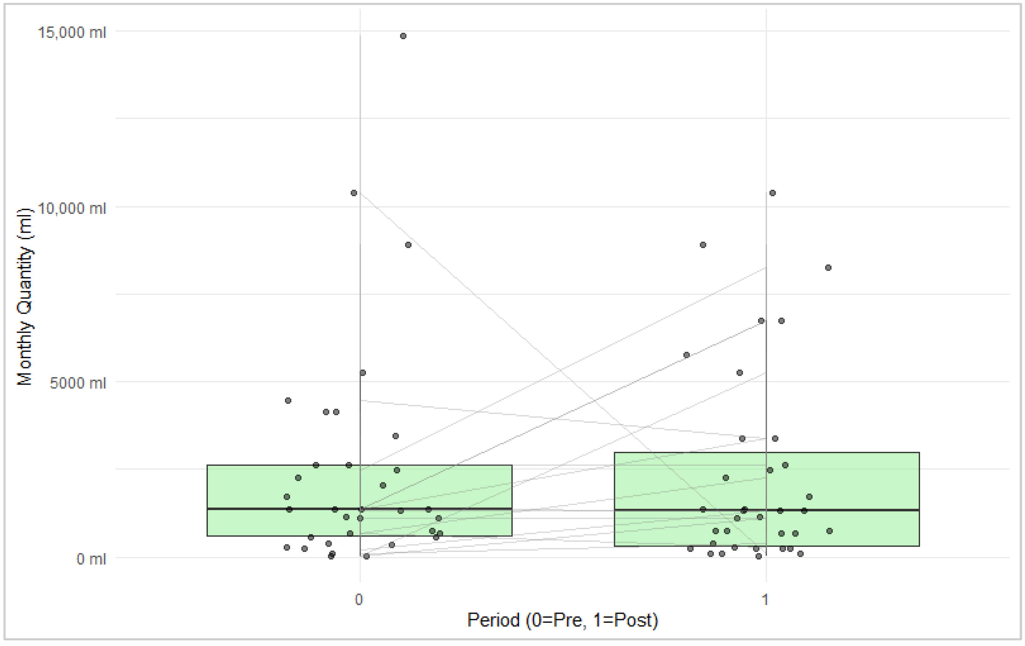
Second, we conducted a sensitivity analysis for outliers. We addressed the concern regarding the limited sample size in the highest-income group (Tier 5). To rule out the possibility that the significant surge in consumption was driven by extreme outliers, we conducted a sensitivity analysis by excluding the top 10% of the subsample and re-estimating the distribution. The systematic upward shift in consumption quantity during the post-policy period persisted even after outlier exclusion (Figure A1 in Appendix A), confirming that the “Elite Surge” reflects a group-wide behavioral response rather than the influence of a few extreme individuals.

Third, we performed placebo tests on non-targeted beverages. To validate that the observed surge in Tier 5 wine consumption was caused by the tax reform and not a result of aggregate economic recovery, we conducted placebo tests on non-targeted beverages (

Table 4. Robustness: Placebo test and falsification tests (impact on non-targeted beverages).

Placebo Beverage	Outcome	ATT	Std. Error	95% CI
Beer	Spending (THB)	−19.3	37	[−91.82, 53.21]
	Frequency (Times/mo)	−0.13	0.08	[−0.28, 0.03]
	Quantity (mL/mo)	−173.16	142.59	[−452.64, 106.32]
	Spend/Time (THB)	11.95	30.25	[−47.34, 71.25]
Whisky	Spending (THB)	20.86	37.23	[−52.12, 93.84]
	Frequency (Times/mo)	0.13	0.08	[−0.03, 0.30]
	Quantity (mL/mo)	151.09	144.81	[−132.74, 434.93]
	Spend/Time (THB)	−2.39	30.28	[−61.74, 56.95]
White Spirits	Spending (THB)	123.02 **	42.27	[40.18, 205.86]
	Frequency (Times/mo)	0.28 ***	0.08	[0.12, 0.45]
	Quantity (mL/mo)	216.89	146.64	[−70.53, 504.31]
	Spend/Time (THB)	87.77 *	39.29	[10.77, 164.77]

Note: Tests replicate the DR-DiD model, assigning placebo beverages as the treatment. Significance levels: * p < 0.05, ** p < 0.01, *** p < 0.001. Source: Authors’ calculation.

).

The results confirm the specificity of the policy shock. For Beer and Whisky, which represent the primary substitutes for wine, we observe null effects across all consumption metrics. The ATT estimates for Spending, Frequency, Quantity, and Expenditure per Occasion for these beverages are statistically indistinguishable from zero. This indicates that the market did not experience a generalized “drinking boom” or aggregate demand shock during the post-policy period.

We observed a statistically significant increase in White Spirit consumption regarding spending and frequency. However, the demographic profile of White Spirit consumers indicates that they are predominantly male (82.52%), report lower average spending, and exhibit a high concentration in the Northeast region (44.06%) relative to the wine cohort. Therefore, this finding is likely attributable to separate, localized economic factors rather than the wine tax policy. The absence of effects for Beer and Whisky, which constitute the primary alternative beverage categories for wine consumers, strongly supports the validity of the identification strategy.

3.4. Net Economic Impact

To evaluate the aggregate utility of the 2024 tax reform, we estimated the Net Economic Impact ($E_{net}$) by combining confirmed fiscal revenue losses with projected marginal increases in social costs. This assessment utilizes the prevalence-based cost-of-illness framework.

The immediate impact of the reform was a direct contraction of state revenue. Ministry of Finance projections at the time of enactment indicated that the reduction in the excise tax rate from 10% to 5%, combined with the elimination of import tariffs, resulted in an annual revenue loss of 579 million THB. This figure constitutes the baseline fiscal cost ($C_{fiscal}$) of the intervention, representing a confirmed transfer of public funds to private consumption.

Beyond fiscal contraction, the policy generates significant externalities by stimulating consumption within a high-value demographic. As detailed in the methodology, the economic cost of alcohol in Thailand is predominantly composed of productivity losses (96.32%), making the burden highly sensitive to the income level of the consumer. Based on our DR-DiD findings, the “additive premiumization” effect was isolated to Tier 5 consumers (income > 100,000 THB). Applying the 9.70× income multiplier to the baseline economic cost raises the economic value-at-risk for a drinker in this tier from the national average of 10,360 THB to approximately 100,455.61 THB per year. When this elevated risk value is applied to the target population of 0.42 million Tier 5 drinkers, who increased their ethanol intake by 28.51% relative to the baseline, the aggregate marginal social cost ($C_{social})$ is estimated at 12,651.80 million THB annually, as shown in

Table 5. Estimated annual Net Economic Cost of the 2024 wine tax reform.

Cost Component	Estimated Value	Data Source/Method
1. Direct Fiscal Cost (Cfiscal)	579	Ministry of Finance Projection
Foregone Revenue (Tariffs + Excise)	579
2. Projected Social Cost (Csocial)	12,072.80	Calculated via HCA Model
Target Population (Ntarget)	0.42	2.64% of Active Drinkers
Baseline Cost per Drinker (Cbaseline)	10,360.08	Luangsinsiri et al. (2023)
Income Valuation Multiplier (Mincome)	9.70×	(Tier 5 Income/Average National Income)
High-Income Adjusted Cost	100,455.61	Cbaseline × 9.70
Marginal Risk Factor (Δrisk)	+28.51%	Derived from DR-DiD
Marginal Cost per Affected Person	28,635.14	(100,455.61 × 28.51%)
Total Net Economic Cost (Enet)	12,651.80	(1 + 2)

Source: Authors’ calculation.

.

3.5. Sensitivity Analysis

We conducted a deterministic sensitivity analysis to evaluate the robustness of the Net Economic Cost estimate by varying three parameters: behavioral response magnitude, income valuation, and the harm function. We tested bounds using 95% confidence intervals, alternated the income multiplier between the specific Tier 5 premium of 9.70 and the national average of 1.0, and applied a convex harm function of 1.5 to model non-linear health risks (Corrao, 2004; Rehm et al., 2010a).

Results confirm a net negative economic impact across all scenarios. The most conservative estimate, which utilizes lower-bound consumption figures and excludes the high-income premium, yields a Net Economic Loss of 1588.25 million THB. This demonstrates that direct fiscal revenue losses exceed even minimal projected social costs. In contrast, the high-impact scenario accounting for non-linear risks among high-value human capital projects an annual loss of 15,258.12 million THB, as presented in

Table 6. Sensitivity analysis of Net Economic Cost.

	Estimated Cost	% Change
Base Case (Mean Intake, Income Multiplier = 9.70)	12,651.80	NA
Lower-Bound Intake, Income Multiplier = 9.70	3515.91	−72.21%
Upper-Bound Intake, Income Multiplier = 9.70	4888.45	−61.36%
Lower-Bound Intake, Income Multiplier = 1	1588.25	−87.45%
Upper-Bound Intake, Income Multiplier = 1	2059.91	−83.72%
Lower-Bound Intake, Income Multiplier = 9.70, Convex Harm = 1.5	15,258.12	20.60%
Upper-Bound Intake, Income Multiplier = 9.70, Convex Harm = 1.5	7043.18	−44.33%
Lower-Bound Intake, Income Multiplier = 1, Convex Harm = 1.5	2092.87	−83.46%
Upper-Bound Intake, Income Multiplier = 1, Convex Harm = 1.5	2800.37	−77.87%

Source: Authors’ calculation.

.

4. Discussion

4.1. Principal Findings: The Regressive Nature of “Premiumization”

The present study utilized a Doubly Robust Difference-in-Differences (DR-DiD) estimator to evaluate the immediate impact of the 2024 excise tax reduction on wine in Thailand. Our findings reveal a distinct dichotomy in policy responsiveness. Contrary to the theoretical expectation that price reductions stimulate broad market demand (Nelson, 2013; Shang et al., 2020), we found no statistically significant changes in consumption frequency or volume among the general population (Income Tiers 1–4). The tax reform failed to lower the effective price floor sufficiently to bridge the affordability gap for low-to-middle-income consumers, for whom wine remains a prohibitive luxury. This null result aligns with the “affordability threshold” hypothesis observed in emerging markets, where price elasticity is often non-linear; below a certain income level, even subsidized luxury goods remain inaccessible regardless of marginal price shifts (Sornpaisarn et al., 2013). Furthermore, evidence suggests that tax reductions on premium goods are frequently absorbed by retailers as profit margins rather than fully passed through to shelf prices, thereby dampening the economic signal for price-sensitive consumers (Ally et al., 2014).

However, a robust behavioral response was identified exclusively among the top income quintile (Tier 5, >100,000 THB/month). For this demographic, the policy functioned as an additive stimulus rather than a simple substitute. While wine consumption volume surged (+1516 mL/month), the analysis detected no statistically significant decline in Beer or Spirit consumption. This indicates that the tax cut did not incentivize consumers to “trade up” (swapping Beer for wine) but rather to expand their alcohol repertoire. Consequently, the policy drove a net accumulation of ethanol intake: affluent consumers maintained their baseline Beer consumption while adding high-ABV wine (12.5%) to their diet. This “additive premiumization” effect creates a “regressive bio-burden,” significantly increasing the total metabolic risk for the socioeconomic elite without the offset that a substitution effect would provide (World Health Organization, 2022).

4.2. Mechanisms: Cross-Price Elasticity and Dietary Shifts

The observed distributional heterogeneity supports the hypothesis that imported wine functions as a Veblen good within the Thai market context; consumption is driven primarily by prestige signaling and exhibits high income elasticity (Fogarty, 2010). For the general population, the demand for wine remained inelastic because the post-tax price point failed to breach the strict affordability threshold characteristic of developing economies (Sornpaisarn et al., 2013). Consequently, the price reduction yielded no utility gain for lower-income groups. However, for high-income earners, the tax cut significantly improved the value proposition of wine relative to other ethanol sources.

This shift in relative prices activated a complex behavioral response best described as an expansion of the alcohol repertoire rather than simple substitution. Affluent consumers leveraged the tax savings to increase the complexity and concentration of their consumption bundle (Gruenewald et al., 2006). This phenomenon aligns with the findings of Gehrsitz et al. (2021), who demonstrated that fiscal incentives favoring specific beverage classes often drive consumers to upgrade the concentration of their intake without reducing total volume. In this instance, the fiscal policy effectively subsidized a transition toward higher ethanol density; it allowed wealthy consumers to accumulate additional metabolic risk by adding high-ABV wine to their diet while maintaining their baseline consumption of lower-ABV beverages.

4.3. Comparison with Global Evidence

The divergence in responsiveness observed between income groups provides empirical weight to the ongoing debate regarding demand heterogeneity in alcohol economics. Conventional meta-analyses, predominantly based on data from high-income OECD nations, suggest that lower-income populations exhibit higher price elasticities of demand due to tighter budget constraints (Nelson, 2013; Wagenaar et al., 2009). Our findings challenge the universality of this axiom. In the context of the Thai market, the null effect observed among lower-income consumers supports the affordability threshold framework proposed by Sornpaisarn et al. (2013). This divergence suggests that in emerging economies, the absolute price floor of imported alcohol remains the primary determinant of consumption, rendering marginal tax adjustments ineffective for market expansion among the poor.

Furthermore, the additive premiumization observed in the high-income tier offers a nuanced counterpoint to the substitution effects typically documented in Western markets. While studies such as Gehrsitz et al. (2021) and Morris et al. (2024) observe clear trade-offs between beverage types based on tax differentials, our data indicate that Thai elites treat wine as a complementary good rather than a substitute. This behavior mirrors patterns observed in markets where Western alcohol serves as a distinct status symbol separate from traditional beverages (Fogarty, 2010). Consequently, policy models derived from European contexts, such as those discussed by Cnossen (2007), may fail to predict behavioral responses in Asian markets where beverage categories are less fungible.

The external validity of these findings is supported by recent evidence from comparable middle-income economies. For instance, Chelwa et al. (2019) estimated price elasticities for wine and Beer in Vietnam and identified a structurally inelastic demand similar to the Thai context. Their findings reinforce the hypothesis that in emerging Southeast Asian economies, consumption is constrained by absolute affordability thresholds rather than marginal price shifts. Furthermore, the psychosocial mechanism driving the observed Elite Surge aligns with Cunningham’s (2023) analysis of premium alcohol markets in South Africa. Cunningham established that status consumption and subjective social norms are the primary determinants of purchase intention for luxury alcohol, whereas perceived affordability exerts a statistically insignificant influence. This parallels our observation that Tier 5 consumers in Thailand responded to the tax cut not as a relief on budget constraints but as a facilitator for status-signaling consumption. On a macro level, these behavioral shifts are consistent with the global convergence trends identified by Holmes and Anderson (2017). Their analysis suggests that as economies transition toward higher income levels, national beverage mixes typically shift away from traditional staples toward globally traded aspirational goods. Our results indicate that fiscal policy can inadvertently accelerate this transition among the wealthy elite while leaving the broader population unchanged.

Finally, the lack of broad market response corroborates the findings of Ally et al. (2014) regarding asymmetric tax pass-through. It is probable that the fiscal benefits were captured within the supply chain for mass-market products, further insulating the price-sensitive consumer from the intended policy signal. This underscores a critical limitation of supply-side tax incentives; without regulatory mandates on pricing, tax reductions rarely translate into consumer surplus for the median earner.

4.4. Fiscal Incidence and Allocative Inefficiency

From a normative public finance perspective, the empirical results uncover a significant structural deficiency in the 2024 fiscal reform. Although the stated objective was to enhance market competitiveness, the outcome constitutes a violation of vertical equity. Theoretical frameworks of optimal taxation, pioneered by Pigou (2020) and refined by O’Donoghue and Rabin (2005), posit that excise taxes on “sin goods” should primarily function to internalize negative externalities while minimizing distortions to consumer welfare. Ideally, the tax burden should be progressive, ensuring that those with higher ability to pay contribute proportionally more to the remediation of social costs (Stiglitz & Rosengard, 2015). In contrast to this theoretical ideal, our empirical data demonstrates that this tax reduction functioned as a regressive fiscal transfer.

Through the enactment of deep cuts on a commodity characterized by high income elasticity of demand, the state effectively subsidized the leisure consumption of the top 2.64% of earners (Tier 5). This demographic emerged as the sole beneficiary of the price reduction, while the fiscal deficit resulting from foregone revenue falls upon the general public. This phenomenon aligns with findings by Cnossen (2007), who argues that ad valorem reductions on premium alcohol categories in developing markets inherently favor the wealthy, as the consumption of such goods is concentrated in the upper socioeconomic strata. Furthermore, as noted by Sornpaisarn et al. (2013) in the Southeast Asian context, demand for imported alcohol among lower-income groups is often constrained by absolute affordability thresholds rather than marginal tax rates. Consequently, the tax cut failed to generate consumer surplus for the median earner and instead facilitated a wealth transfer to the demographic with the highest ability to pay (Gruber & Kőszegi, 2004).

These findings can be interpreted theoretically through the framework of the Laffer Curve. The implicit rationale for the tax cut assumed that existing wine tax rates were situated on the prohibitive or right side of the Laffer peak, where excessive rates suffocate demand to such an extent that a rate reduction would stimulate sufficient volume growth to maintain or even increase total revenue (Umer, 2018). Our empirical results contradict this assumption. Wang et al. (2017) argue that consumption tax cuts in open economies can theoretically generate a “Dynamic Laffer Effect” by stimulating domestic demand booms (Wang et al., 2017). Our data indicates that this stimulus was structurally confined in the present case. The aggregate volume growth was insufficient to offset the lower tax rate because the expenditure switching effect was limited exclusively to the high-income Tier 5.

This outcome aligns with the microeconomic evidence presented by Gamarra Rondinel et al. (2024), who demonstrate that a net fiscal loss results when the “Mechanical Effect” (revenue loss from the rate cut) exceeds the “Behavioral Effect” (revenue gain from increased activity). The inelastic demand observed among the majority of the population (Tiers 1–4) meant the behavioral response was too weak to generate a Laffer-style recovery. Sentinelo et al. (2025) suggest that smaller economies often operate on the ascending slope of the curve, where fiscal effort is not yet self-defeating (Sentinelo et al., 2025). Our findings confirm that the pre-reform tax rate was likely situated within this normal range. The policy consequently functioned not as a revenue-optimizing stimulus but as a simple revenue-sacrificing tax break.

The inefficiency of this policy is quantified by the stark disproportion between fiscal costs and economic losses. As calculated in our Results Section, the economy incurs approximately 21.85 THB in projected social costs and fiscal deficits for every 1 THB of tax relief provided to the wealthy. This ratio suggests that the policy acts as a “reverse deadweight loss.” In standard public economics, a deadweight loss occurs when taxation discourages mutually beneficial trade (Chetty, 2009). Here, however, the government forfeits revenue (579 million THB) not to correct a market failure, but to subsidize risk accumulation. This diversion of resources represents a high opportunity cost, as these funds are removed from potential public health investments or progressive redistribution mechanisms (Cook & Moore, 2002). The reform, therefore, exacerbates allocative inefficiency by incentivizing the consumption of demerit goods among the most economically productive segment of the population.

4.5. Methodological Considerations and Limitations

4.5.1. Sample Size and Representativeness

The analytical sample size of 834 participants represents a limitation relative to the total Thai population. While a larger sample would be required to generate precise national prevalence estimates for all demographic subgroups, the primary objective of this study was to identify causal behavioral shifts rather than baseline prevalence. The multi-stage stratified cluster sampling design was rigorously implemented to ensure that the study covered all five geographic regions and adhered to population-proportional quotas for urbanicity and gender despite the restricted sample size. Furthermore, the statistical power of the Doubly Robust Difference-in-Differences (DR-DiD) estimator relies on the magnitude of the effect size. The substantial behavioral response observed in the highest income tier was large enough to be detected with statistical significance even within this sample frame. We caution against generalizing these findings to the entire national population without sampling weights; nevertheless, the internal validity of the threshold effect among high-income earners remains robust. The clear divergence between the highest income tier and the lower tiers suggests that the observed phenomenon is not an artifact of sampling error but a reflection of genuine economic heterogeneity.

4.5.2. Self-Reporting and Recall Bias

The reliance on retrospective self-reported data introduces potential recall bias. We mitigated this risk through three layers of verification. First, procedurally, the survey utilized major cultural anchors, specifically the Songkran Festival in April and the New Year holidays, to strictly delimit the pre-policy and post-policy reporting windows, aiding memory retrieval. Second, statistically, we addressed the concern that recall errors might manifest as extreme values by conducting the sensitivity analysis detailed in Section 3.3. The persistence of the “Elite Surge” effect even after excluding the top 10% of outliers confirms that the findings are not driven by sporadic reporting artifacts. Third, we tested for Common Method Bias (CMB) using Harman’s Single-Factor Test. An exploratory factor analysis containing all key variables (consumption metrics and demographics) showed that a single factor explained only 27.4% of the total variance, which is substantially below the 50% threshold.

Methodologically, the Doubly Robust Difference-in-Differences (DR-DiD) estimator explicitly controls for time-invariant reporting heterogeneity. This framework integrates Inverse Probability Weighting with Outcome Regression to ensure that baseline differences in reporting tendencies between groups are neutralized provided they remain constant over time (Greenfield & Kerr, 2008). Crucially, the validity of the data is supported by the specific behavioral pattern observed. If the findings were driven by random recall error, we would expect a uniform distribution of noise across all beverages. Instead, the analysis reveals a structured additive premiumization effect where wine consumption surged while Beer consumption remained statistically stable or declined slightly. This specific behavioral structure aligns with economic theory regarding luxury goods rather than memory artifact. Nevertheless, self-reported alcohol consumption is historically under-reported. Consequently, the ethanol intake levels presented here should be interpreted as conservative lower-bound estimates (Rehm et al., 2020).

4.5.3. Temporal Scope and Confounding Factors

The evaluation window covers the immediate ten-month period following the policy implementation. Economic theory suggests that long-run price elasticities often exceed short-run estimates due to habit formation (Grossman et al., 1995). Consequently, the ethanol load observed among high-income earners may intensify over time as the consumption of high-ABV wine becomes normalized within this demographic. Additionally, this study focuses exclusively on domestic health impacts and does not evaluate the stated goal of the policy to boost tourism revenue. From a public health nutrition perspective, however, the domestic metabolic burden remains the priority regardless of tourism outcomes.

Regarding the attribution of causality, we acknowledge the potential confounding role of broader socioeconomic shifts, such as post-pandemic lifestyle changes or shifting consumer preferences. However, the use of the DR-DiD estimator mitigates this concern by identifying a control group (Beer and Spirit consumers) exposed to the same macroeconomic environment, the model isolates the policy shock from slowly evolving lifestyle trends. The divergence in behavior specific to the high-income tier, occurring precisely within the ten-month post-policy window, supports the conclusion that the effect is driven by the tax-induced price mechanism rather than general socioeconomic drift.

Finally, while the analysis accounts for legal market consumption, it does not explicitly track unrecorded or illicit alcohol. The elimination of import tariffs theoretically reduces the economic incentive for smuggling, suggesting that any bias from unrecorded trade would likely result in an underestimation rather than an overestimation of the legal market expansion (Rehm et al., 2010b).

5. Conclusions and Recommendations

5.1. Conclusions

The empirical evaluation of Thailand’s 2024 wine tax reform reveals a fundamental misalignment between fiscal objectives and behavioral reality. While the policy was designed to stimulate aggregate demand and tourism spending, our causal analysis utilizing the Doubly Robust Difference-in-Differences estimator demonstrates that the tax reduction failed to generate broad market expansion. For the vast majority of the population (income Tiers 1 to 4), the price elasticity of demand for imported wine remained unresponsive to the tax cut, confirming that the absolute price floor of luxury beverages in emerging markets acts as a binding constraint regardless of marginal fiscal adjustments.

Instead of a generalized economic stimulus, the reform functioned as a regressive fiscal transfer. The behavioral response was concentrated exclusively among the top 2.64% of income earners, who leveraged the tax relief to increase their net ethanol intake through additive premiumization. This distributional distortion resulted in severe allocative inefficiency. Our economic impact assessment estimates that the policy generates a Net Economic Loss of approximately 12,651.80 million THB annually. This deficit is driven by the divergence between the confirmed fiscal cost of foregone revenue and the projected social externalities associated with increased alcohol consumption among high-value human capital. Specifically, the Thai economy incurs approximately 21.85 THB in projected productivity losses and fiscal deficits for every 1 THB of tax relief provided to the wealthy.

These findings suggest that supply-side tax incentives for positional goods represent a suboptimal strategy for economic stimulation in developing economies. The reliance on ad valorem excise mechanisms decoupled the tax liability from the biological externality, effectively subsidizing higher-risk consumption patterns among the elite. To correct this market failure, future fiscal policy should prioritize a structural transition toward specific volumetric taxation. By basing tax liability strictly on ethanol content rather than commercial value, the state can internalize the social costs of consumption, neutralize the regressive subsidies currently enjoyed by high-income earners, and ensure that fiscal policy supports rather than undermines national economic resilience.

5.2. Policy Recommendations: The Case for Volumetric Taxation

The findings of this study underscore the structural limitations of ad valorem (value-based) excise systems in mitigating public health harms. By reducing the tax burden on wine based on its commercial classification rather than its toxicological content, the current policy framework inadvertently incentivizes the consumption of beverages with higher ethanol density (Sornpaisarn et al., 2013). From a theoretical standpoint, this misalignment violates the Pigouvian principle of efficient taxation, which posits that fiscal interventions should directly target the source of the negative externality to minimize market distortion (Griffith et al., 2019). Given that the external cost in alcohol control is driven by the volume of ethanol consumed rather than the monetary value of the product, ad valorem systems fail to internalize the specific health risks associated with higher alcohol concentrations.

The observation that modest tax shocks can yield null aggregate effects is consistent with recent work on inference in Difference-in-Differences with few treated clusters (MacKinnon & Webb, 2020). Our results reinforce the notion that a pattern of null effects for the majority alongside detectable effects for a small subset is plausible when policy shocks are modest and affect segments with higher income elasticity and status-signaling motives. This underscores the need for tax instruments that are robust to distributional heterogeneity.

We recommend a transition toward a volumetric taxation model to align fiscal policy with public health nutrition objectives. Under this regime, tax liability is determined strictly by the grams of pure ethanol contained in the product irrespective of beverage type or price. This specific taxation approach creates a direct correlation between tax liability and biological harm, effectively neutralizing the price advantages currently enjoyed by high-ABV wine relative to lower-ABV alternatives (Chaloupka et al., 2019). Structural evidence from wine markets suggests that ad valorem taxes (based on price) and specific volumetric taxes have divergent effects on consumption and distribution (Bonnet et al., 2025). Ad valorem taxes such as those reduced in the 2024 Thai reform can inadvertently encourage premiumization by lowering the relative price of high-value high-ABV products for affluent consumers without discouraging total ethanol intake.

Reliance on ad valorem taxes exposes public health outcomes to industry pricing strategies as producers can absorb tax hikes or lower pre-tax prices to maintain affordability. Specific volumetric taxes or Minimum Unit Pricing (MUP) are more effective at establishing a price floor that targets the heaviest drinkers and the cheapest high-strength beverages. Bonnet et al. (2025) demonstrate that MUP can be particularly effective in reducing total ethanol purchases while mitigating the trading-up or premiumization channels observed in our high-income cohort. Integrating these instruments into the Thai tax code could correct the misalignment between fiscal policy and public health objectives, ensuring that the cost of alcohol reflects its toxicological load rather than its prestige value.

References

1. Ally, A. K., Meng, Y., Chakraborty, R., Dobson, P. W., Seaton, J. S., Holmes, J., Angus, C., Guo, Y., Hill-McManus, D., Brennan, A., & Meier, P. S. (2014). Alcohol tax pass-through across the product and price range: Do retailers treat cheap alcohol differently? Addiction, 109(12), 1994–2002. [Google Scholar] [CrossRef] [PubMed]
2. Bonnet, C., Etile, F., & Lecocq, S. (2025). Minimum pricing or volumetric taxation? Quantity, quality and competition effects of price regulations in alcohol markets. HAL. [Google Scholar] [CrossRef]
3. Chaloupka, F. J., Powell, L. M., & Warner, K. E. (2019). The use of excise taxes to reduce tobacco, alcohol, and sugary beverage consumption. Annual Review of Public Health, 40(1), 187–201. [Google Scholar] [CrossRef] [PubMed]
4. Chelwa, G., Toan, P. N., Hien, N. T. T., Thu, L. T., Anh, P. T. H., & Ross, H. (2019). Do beer and wine respond to price and tax changes in Vietnam? Evidence from the Vietnam household living standards survey. BMJ Open, 9(5), e027076. [Google Scholar] [CrossRef]
5. Chetty, R. (2009). Is the taxable income elasticity sufficient to calculate deadweight loss? The implications of evasion and avoidance. American Economic Journal: Economic Policy, 1(2), 31–52. [Google Scholar] [CrossRef]
6. Cnossen, S. (2007). Alcohol taxation and regulation in the European Union. International Tax and Public Finance, 14(6), 699–732. [Google Scholar] [CrossRef]
7. Cook, P. J., & Moore, M. J. (2002). The economics of alcohol abuse and alcohol-control policies. Health Affairs, 21(2), 120–133. [Google Scholar] [CrossRef]
8. Corrao, G. (2004). A meta-analysis of alcohol consumption and the risk of 15 diseases. Preventive Medicine, 38(5), 613–619. [Google Scholar] [CrossRef]
9. Cunningham, N. (2023). The role of social group influences when intending to purchase premium alcohol. Cogent Business & Management, 10(1), 2174093. [Google Scholar] [CrossRef]
10. Elder, R. W., Lawrence, B., Ferguson, A., Naimi, T. S., Brewer, R. D., Chattopadhyay, S. K., Toomey, T. L., & Fielding, J. E. (2010). The effectiveness of tax policy interventions for reducing excessive alcohol consumption and related harms. American Journal of Preventive Medicine, 38(2), 217–229. [Google Scholar] [CrossRef]
11. Fogarty, J. (2010). The demand for beer, wine and spirits: A survey of the literature. Journal of Economic Surveys, 24(3), 428–478. [Google Scholar] [CrossRef]
12. Gallet, C. A. (2007). The demand for alcohol: A meta-analysis of elasticities. Australian Journal of Agricultural and Resource Economics, 51(2), 121–135. [Google Scholar] [CrossRef]
13. Gamarra Rondinel, A., Sanz-Sanz, J. F., & Arrazola, M. (2024). The individual laffer curve: Evidence from the Spanish income tax. Empirical Economics, 67(6), 2719–2769. [Google Scholar] [CrossRef]
14. Gehrsitz, M., Saffer, H., & Grossman, M. (2021). The effect of changes in alcohol tax differentials on alcohol consumption. Journal of Public Economics, 204, 104520. [Google Scholar] [CrossRef]
15. Greenfield, T. K., & Kerr, W. C. (2008). Alcohol measurement methodology in epidemiology: Recent advances and opportunities. Addiction, 103(7), 1082–1099. [Google Scholar] [CrossRef]
16. Griffith, R., O’Connell, M., & Smith, K. (2019). Tax design in the alcohol market. Journal of Public Economics, 172, 20–35. [Google Scholar] [CrossRef]
17. Grossman, M., Chaloupka, F. J., & Sirtalan, I. (1995). An empirical analysis of alcohol addiction: Results from the monitoring the future panels. National Bureau of Economic Research, 36, 39–48. Available online: https://ssrn.com/abstract=225264 (accessed on 12 January 2026).
18. Groves, R. M., Fowler, F. J., Couper, M., Lepkowski, J. M., Singer, E., & Tourangeau, R. (2009). Survey methodology. Wiley. [Google Scholar]
19. Gruber, J., & Kőszegi, B. (2004). Tax incidence when individuals are time-inconsistent: The case of cigarette excise taxes. Journal of Public Economics, 88(9–10), 1959–1987. [Google Scholar] [CrossRef]
20. Gruenewald, P. J., Ponicki, W. R., Holder, H. D., & Romelsjö, A. (2006). Alcohol prices, beverage quality, and the demand for alcohol: Quality substitutions and price elasticities. Alcoholism: Clinical and Experimental Research, 30(1), 96–105. [Google Scholar] [CrossRef]
21. Holmes, A. J., & Anderson, K. (2017). Convergence in national alcohol consumption patterns: New global indicators. Journal of Wine Economics, 12(2), 117–148. [Google Scholar] [CrossRef]
22. Kosulwat, V. (2002). The nutrition and health transition in Thailand. Public Health Nutrition, 5(1a), 183–189. [Google Scholar] [CrossRef] [PubMed]
23. Luangsinsiri, C., Youngkong, S., Chaikledkaew, U., Pattanaprateep, O., & Thavorncharoensap, M. (2023). Economic costs of alcohol consumption in Thailand, 2021. Global Health Research and Policy, 8(1), 51. [Google Scholar] [CrossRef] [PubMed]
24. MacKinnon, J. G., & Webb, M. D. (2020). Randomization inference for difference-in-differences with few treated clusters. Journal of Econometrics, 218(2), 435–450. [Google Scholar] [CrossRef]
25. Ministry of Interior. (2024). Population statistics. Available online: https://stat.bora.dopa.go.th/stat/statnew/statMONTH/statmonth/#/mainpage (accessed on 10 January 2026).
26. Ministry of Public Health. (2024). Public health statistics 2007–2024. Available online: https://spd.moph.go.th/illness-report/ (accessed on 10 January 2026).
27. Morris, D., Angus, C., Gillespie, D., Stevely, A. K., Pryce, R., Wilson, L., Henney, M., Meier, P. S., Holmes, J., & Brennan, A. (2024). Estimating the effect of transitioning to a strength-based alcohol tax system on alcohol consumption and health outcomes: A modelling study of tax reform in England. The Lancet Public Health, 9(10), e719–e728. [Google Scholar] [CrossRef]
28. National Statistical Office. (2021). The 2021 health behaviour of population survey. National Statistical Office. [Google Scholar]
29. National Statistical Office. (2022). The 2021 household socio-economic survey. Available online: https://www.nso.go.th/nsoweb/storage/survey_detail/2023/20230503192425_47888.pdf (accessed on 5 January 2026).
30. Nelson, J. P. (2013). Meta-analysis of alcohol price and income elasticities—With corrections for publication bias. Health Economics Review, 3(1), 17. [Google Scholar] [CrossRef]
31. O’Donoghue, T., & Rabin, M. (2005). Optimal taxes for sin goods. Swedish Economic Policy Review, 12, 7–39. [Google Scholar]
32. Office of the National Economic and Social Development Council. (2025). Decile by income (1988–2023). Office of the National Economic and Social Development Council (NESDC), Office of the Prime Minister, Thailand. [Google Scholar]
33. Pigou, A. (2020). The economics of welfare. Palgrave Macmillan. [Google Scholar]
34. Podsakoff, P. M., MacKenzie, S. B., Lee, J.-Y., & Podsakoff, N. P. (2003). Common method biases in behavioral research: A critical review of the literature and recommended remedies. Journal of Applied Psychology, 88(5), 879–903. [Google Scholar] [CrossRef]
35. Pritchard, C., & Sculpher, M. J. (2000). Productivity costs: Principles and practice in economic evaluation. Office of Health Economics. [Google Scholar]
36. Rehm, J., Baliunas, D., Borges, G. L. G., Graham, K., Irving, H., Kehoe, T., Parry, C. D., Patra, J., Popova, S., Poznyak, V., Roerecke, M., Room, R., Samokhvalov, A. V., & Taylor, B. (2010a). The relation between different dimensions of alcohol consumption and burden of disease: An overview. Addiction, 105(5), 817–843. [Google Scholar] [CrossRef]
37. Rehm, J., Crépault, J., Wettlaufer, A., Manthey, J., & Shield, K. (2020). What is the best indicator of the harmful use of alcohol? A narrative review. Drug and Alcohol Review, 39(6), 624–631. [Google Scholar] [CrossRef]
38. Rehm, J., Kanteres, F., & Lachenmeier, D. W. (2010b). Unrecorded consumption, quality of alcohol and health consequences. Drug and Alcohol Review, 29(4), 426–436. [Google Scholar] [CrossRef]
39. Rice, D. P., & Cooper, B. S. (1967). The economic value of human life. American Journal of Public Health and the Nations Health, 57(11), 1954–1966. [Google Scholar] [CrossRef] [PubMed]
40. Sant’Anna, P. H. C., & Zhao, J. (2020). Doubly robust difference-in-differences estimators. Journal of Econometrics, 219(1), 101–122. [Google Scholar] [CrossRef]
41. Scheaffer, R. L., Mendenhall, W., Ott, R. L., & Gerow, K. (2012). Elementary survey sampling. Brooks/Cole. [Google Scholar]
42. Sentinelo, T., Queirós, M., Oliveira, J. M., & Ramos, P. (2025). Tax Optimization in the European Union: A laffer curve perspective. Economies, 13(12), 359. [Google Scholar] [CrossRef]
43. Shang, C., Ngo, A., & Chaloupka, F. J. (2020). The pass-through of alcohol excise taxes to prices in OECD countries. The European Journal of Health Economics, 21(6), 855–867. [Google Scholar] [CrossRef]
44. Sornpaisarn, B., Shield, K., Cohen, J., Schwartz, R., & Rehm, J. (2013). Elasticity of alcohol consumption, alcohol-related harms, and drinking initiation in low- and middle-income countries: A systematic review and meta-analysis. The International Journal of Alcohol and Drug Research, 2(1), 45–58. [Google Scholar] [CrossRef]
45. Stiglitz, J. E., & Rosengard, J. K. (2015). Economics of the public sector. W.W. Norton & Company, Inc. [Google Scholar]
46. The Secretariat of the Cabinet. (2024). Resolution on excise tax and import tariff reduction for wine. Available online: https://resolution.soc.go.th/?prep_id=410191 (accessed on 20 December 2025).
47. Umer, H. (2018). Fairness-adjusted laffer curve: Strategy versus direct method. Games, 9(3), 56. [Google Scholar] [CrossRef]
48. Wagenaar, A. C., Salois, M. J., & Komro, K. A. (2009). Effects of beverage alcohol price and tax levels on drinking: A meta-analysis of 1003 estimates from 112 studies. Addiction, 104(2), 179–190. [Google Scholar] [CrossRef]
49. Wang, W., Wang, Y., & Wang, J. (2017). Do consumption tax cuts lead to dynamic laffer effects in open economies? Theoretical Economics Letters, 7(3), 324–338. [Google Scholar] [CrossRef][Green Version]
50. World Health Organization. (2002). International guide for monitoring alcohol consumption and related harm. World Health Organization. [Google Scholar]
51. World Health Organization. (2017). Tackling NCDs: “Best buys” and other recommended interventions for the prevention and control of noncommunicable diseases. World Health Organization. [Google Scholar]
52. World Health Organization. (2018). Global status report on alcohol and health 2018. World Health Organization. [Google Scholar]
53. World Health Organization. (2022). The potential value of minimum pricing for protecting lives no place for cheap alcohol. World Health Organization. [Google Scholar]
Figure 1. Consumption trends by beverage type. Source: Authors’ calculation.
Economies 14 00056 g001
Figure 2. Heterogeneous treatment effects of wine tax reform on consumption by income tier (DR-DiD Estimates). Source: Authors’ calculation.
Economies 14 00056 g002