Stock Market Development, Economic Growth and Environmental Sustainability in South Africa: A Cointegration and Time–Frequency Analysis

Abstract

The development of stock markets can influence both economic growth and environmental sustainability, yet whether financial market expansion can achieve these objectives simultaneously remains unclear in emerging economies. This study examines the effects of stock market development (SMD) on economic growth and carbon emissions in South Africa over 1975–2022 using autoregressive distributed lag (ARDL) models and wavelet coherence analysis. The ARDL estimates reveal predominantly negative or insignificant effects on economic growth, while nonlinear specifications indicate that positive growth effects emerge at higher levels of market development. Similarly, market capitalization and trading activity increasingly exhibit positive associations with carbon emissions after 1994, suggesting that financial deepening can reinforce emission-intensive economic activity. In contrast, greater market breadth is associated with lower emissions. Wavelet coherence further demonstrates substantial time- and frequency-dependent relationships, with post-1994 financial integration marking stronger stock market–growth and stock market–emission linkages. Short-run emission reductions during major crises appear temporary, reflecting contractions in economic and market activity. These findings suggest that stock market expansion alone cannot deliver sustainable growth. Policy should therefore ‘green’ financial development by directing capital toward renewable energy, clean technologies, and low-carbon firms while strengthening ESG disclosure, environmental compliance, and climate-related financial regulation.

1. Introduction

In recent years, global policymakers have increasingly acknowledged the dual role of stock markets in advancing the Sustainable Development Goals (SDGs). On one hand, stock markets are recognized for their traditional role in fostering economic growth by mobilizing financial assets and channeling funds from surplus to deficit units. This process supports asset accumulation, capital formation, and productivity growth (Levine & Zervos, 1998; Rousseau & Wachtel, 2000; Arestis et al., 2001; Ang, 2008; Damasceno & Guedes, 2024), aligning with SDG 8’s goal of promoting sustainable economic growth (https://sdgs.un.org/goals/goal8, accessed on 21 July 2026). Concurrently, stock markets are under pressure to integrate environmental, social, and governance (ESG) considerations into corporate practices, introducing ‘green’ financial instruments that facilitate investment in sustainable projects. This role corresponds with SDG 13’s imperative to combat climate change (https://sdgs.un.org/goals/goal13, accessed on 21 July 2026) (Acheampong et al., 2020; Tan et al., 2025).

Whilst African countries have been historically characterized by underdeveloped and illiquid equity markets, South Africa is a notable exception, having experienced disparate stock market development. The Johannesburg Stock Exchange (JSE), established in 1887, contrasts sharply with many African exchanges emerging a century later in the 1990s (Phiri, 2015; Nyasha & Odhiambo, 2015). Technologically advanced with sophisticated trading platforms like algorithmic and high-frequency trading, the JSE stands out amidst less developed counterparts, underpinned by robust infrastructure and stringent regulatory frameworks lacking in other African nations (Phiri, 2020). The JSE boasts over 400 listed companies, with a market capitalization exceeding $1.07 trillion, surpassing combined totals of other frontier African markets (Ngare et al., 2014). South Africa’s market capitalization-to-GDP ratio exceeds 320%, significantly outpacing industrialized equity markets in G7 countries (Canada 141%, France 127%, Germany 47%, Japan 146%, US 200%, UK 70%). However, this stock market prominence is juxtaposed against South Africa’s substantial carbon emissions, primarily from coal, which account for approximately 60% of Africa’s emissions (Shahbaz et al., 2013; Ganda, 2018; Phiri & Nyoni, 2023; Phiri et al., 2024).

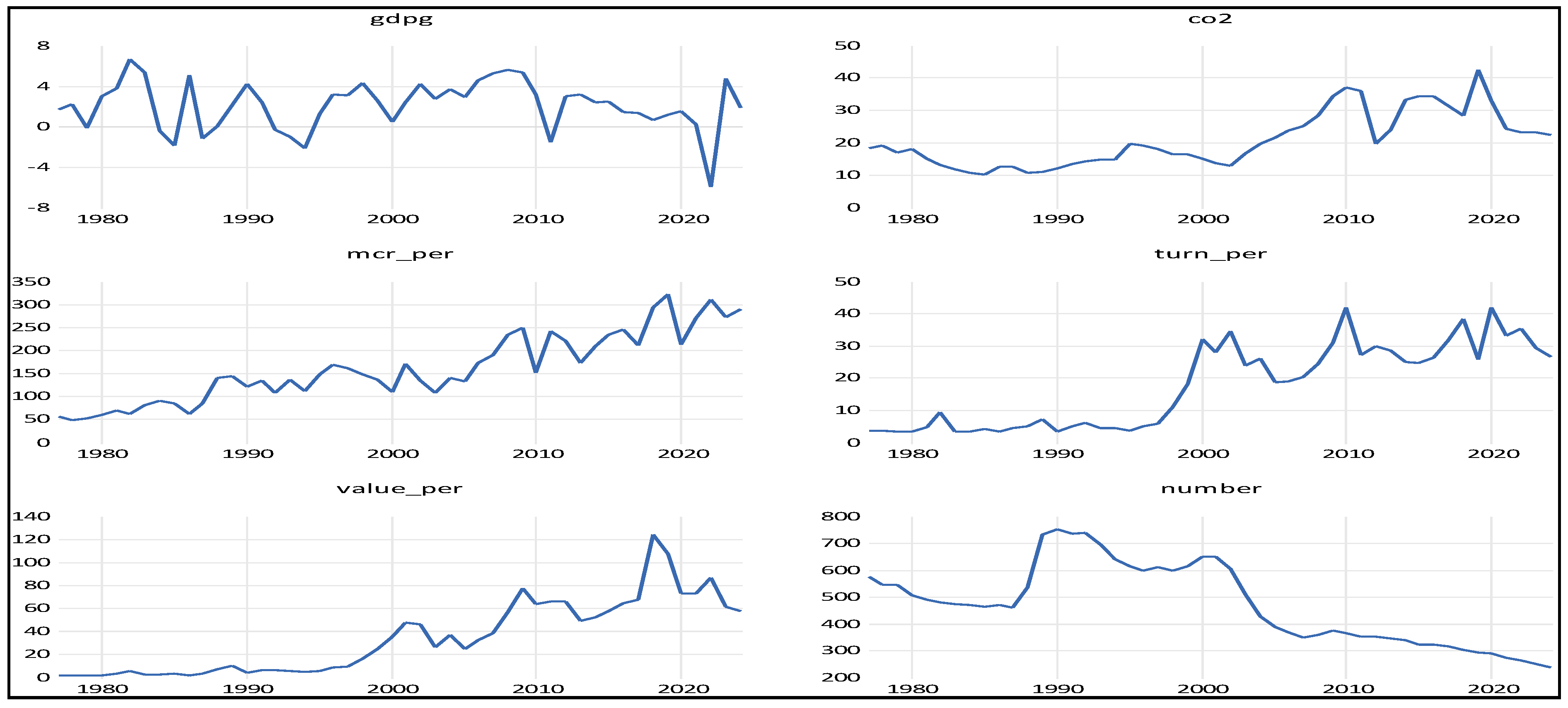
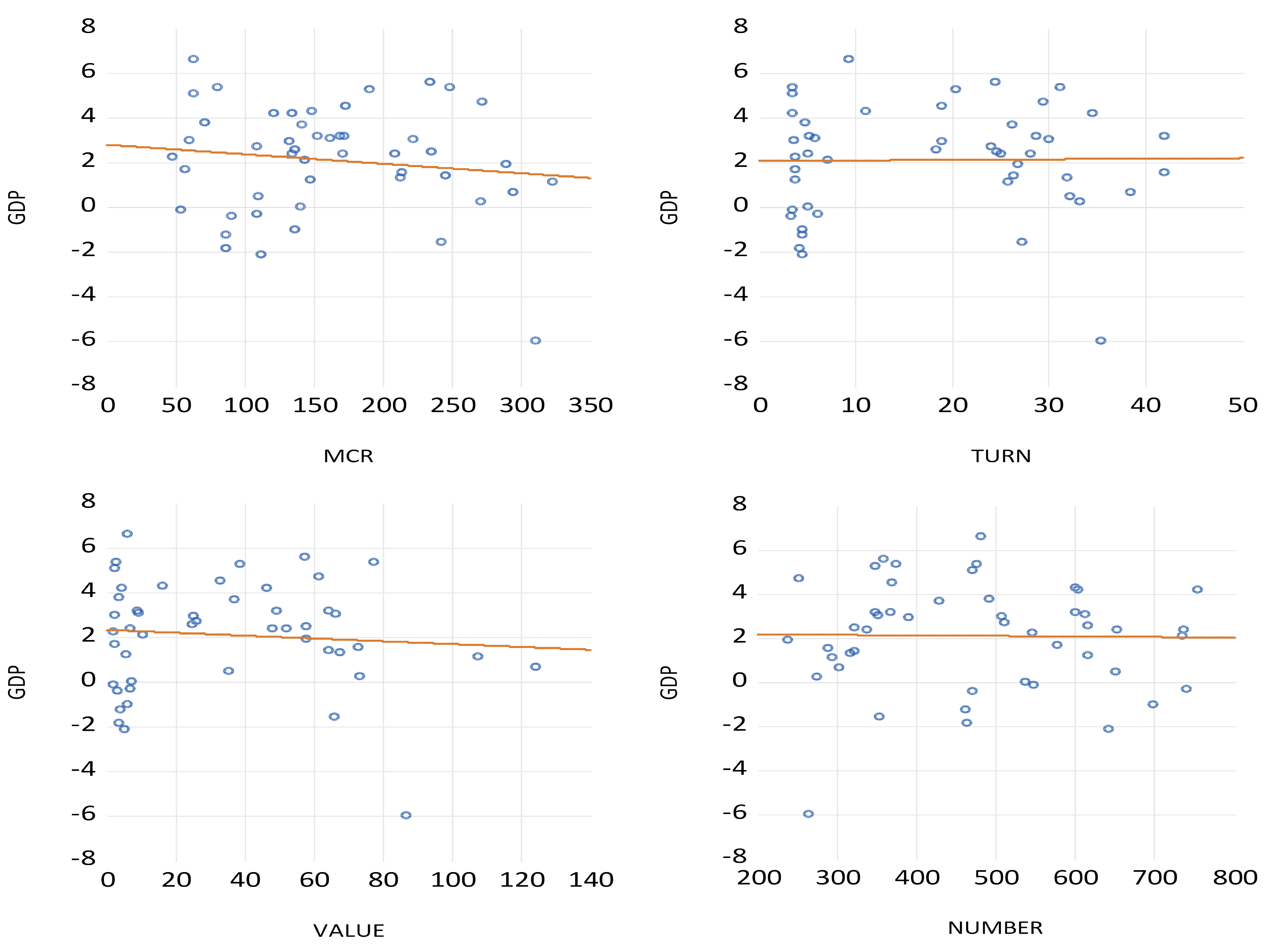
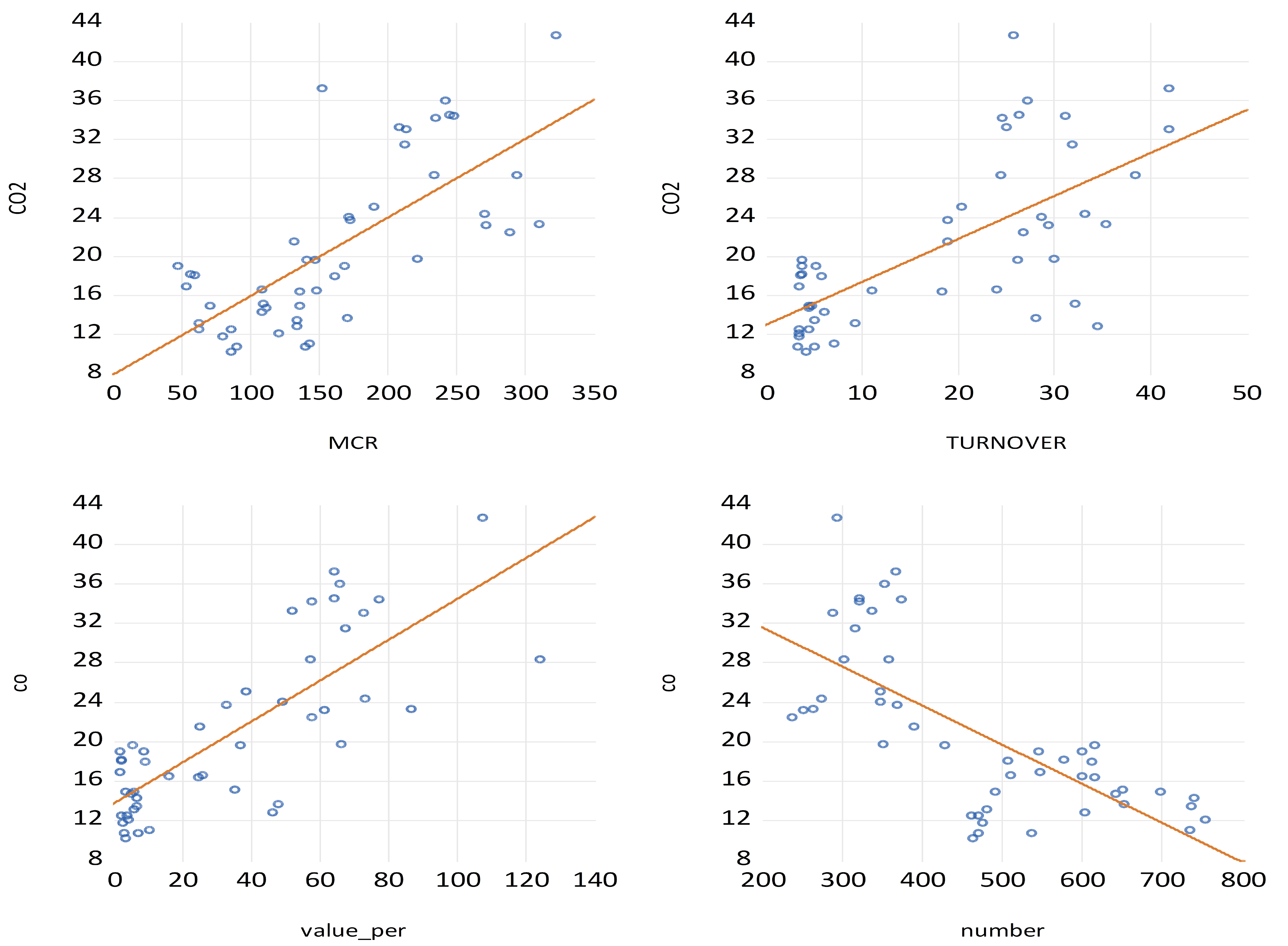
Recent World Bank data reveals that, except for the number of listed firms, South Africa’s stock market development metrics (i.e., market capitalization ratio, stock traded value ratio, and stock market turnover ratio) have gradually increased since 1994. In contrast, GDP and carbon emissions have shown greater volatility, notably during post-2010 recession periods (see Figure 1). The scatterplot correlations between stock market activity and GDP growth (carbon emissions) depicted in Figure 2 (Figure 3) reveal varied relationships, challenging the conventional views of positive stock market–growth and negative stock market–emission associations (Rousseau & Wachtel, 2000; Beck & Levine, 2004; Tamazian et al., 2009; Mhadhbi et al., 2021). Specifically, evidence for South Africa’s stock market–growth relationship is inconclusive (Ndako, 2010; Phiri, 2015; Nyasha & Odhiambo, 2015), while research on the stock market–emission relationship remains virtually nonexistent. The central problem of our study, therefore, is determining whether stock market development in South Africa can promote economic growth without exacerbating environmental degradation.

Further scrutiny of Figure 1 highlights non-monotonic trends in stock market activity, economic growth, and carbon emissions. Structural breaks, such as South Africa’s democratization in 1994 and subsequent economic integration, alongside market reforms like the ‘Big Bang’ of 1995 and advanced trading systems, mark significant shifts in stock market dynamics (Mkhize & Msweli-Mbanga, 2006). Recessionary periods, including the global financial crisis of 2007–2009 and the 2020 COVID-19 pandemic, similarly impact economic indicators and emissions. Stock market activity exhibits cyclical patterns with pronounced expansions and contractions, contrasting with less volatile economic growth and emission data. The existing literature primarily employs linear models, overlooking these asymmetries; recent studies using nonlinear techniques highlight these nuances (Phiri, 2015; Mhadhbi et al., 2021; Masten et al., 2008; Cave et al., 2020). Nonetheless, there exists an empirical gap in investigating the nonlinear relationship between stock market development, economic growth and carbon emissions in South Africa.

Against this backdrop, we re-evaluate the impact of stock market development on economic growth and environmental degradation in South Africa using both autoregressive distributed lag (ARDL) regressions and wavelet coherence analysis. The ARDL approach remains a widely employed econometric technique for examining linear cointegration in stock market–growth and stock market–emission relationships (Nyasha & Odhiambo, 2015; Ananwude & Osakwe, 2017; Thaddeus et al., 2024; Sharma et al., 2021; R. Zhang et al., 2022). Extending this framework, we incorporate nonlinearities by estimating kinked ARDL models that include squared terms of stock market indicators in growth regressions. Complementing this, wavelet coherence analysis offers a more flexible and powerful tool to explore the co-movement between time series in the time–frequency domain. This method captures the sign, strength, and direction of dynamic relationships on a scale-by-scale basis, thereby allowing us to identify time-varying, cyclical, and asymmetric patterns of causality. While wavelet methods have recently gained prominence in the financial development literature, mainly being applied to explore co-movements with carbon emissions (Hung, 2023; Subhan et al., 2023), renewable energy consumption (L. T. Ha, 2022), and human capital (N. M. Ha et al., 2023), they remain largely unexplored in the context of stock market–growth and stock market–emission linkages.

Our study makes several novel contributions to the literature. Firstly, we jointly examine the stock market–growth and stock market–emission relationships in a single analysis, thereby bridging two empirical strands and addressing the central policy question: can stock market development in South Africa support both economic growth and environmental sustainability? Secondly, we pioneer the application of wavelet coherence to these relationships, offering time–frequency insights that help reconcile previously inconsistent findings. Thirdly, beyond conventional measures of stock market activity (i.e., market capitalization, traded value, and turnover) we incorporate the number of listed firms, a dimension often overlooked. Notably, listings on the JSE have declined by over 50% since the 1990s, largely due to rising compliance and reporting costs under the King Codes and CSR frameworks (De Beer et al., 2015; Keyser et al., 2020; Pask, 2024). We explore whether this decline in listed firms enhances or hinders economic growth and environmental outcomes in South Africa.

We structure the remainder of this paper as follows: Section 2 outlines our empirical framework and estimation methods. Section 3 describes our data and provides an initial overview of time series trends. Section 4 presents our empirical analyses, and Section 5 concludes with policy implications and avenues for future research.

2. Literature Review

2.1. Stock Market–Growth Nexus

The theoretical link between stock markets and economic growth is well-established in endogenous growth models incorporating financial contracts. In Levine’s (1991, 1997) model, equity markets mitigate liquidity and productivity risks, enhancing firm efficiency and long-term capital accumulation. Bencivenga et al. (1996) emphasize that liquid secondary markets reduce the cost of premature asset liquidation, encouraging investment in long-term, high-yield projects. Greenwood and Smith (1997) extend this by modeling the endogenous emergence of equity markets when their participation costs fall below bank trading costs, showing that markets enhance capital allocation and specialization. Boyd and Smith (1998) propose a threshold model where equity markets emerge as economies mature, suggesting a nonlinear growth effect.

Empirically, early panel studies (Rousseau & Wachtel, 2000; Beck & Levine, 2004) found a positive stock market–growth relationship, including for South Africa. However, the results become mixed when distinguishing between developed and developing economies (e.g., Fufa & Kim, 2018) or focusing on African countries (Adjasi & Biekpe, 2006; Enisan & Olufisayo, 2009). Country-specific studies on South Africa are similarly inconclusive: while some find no significant relationship (Nyasha & Odhiambo, 2015), others report positive effects (Ndako, 2010; Phiri, 2015; Osakwe et al., 2020). These inconsistencies often stem from differences in estimation periods and the limitations of linear models (e.g., OLS, GMM, ARDL), which fail to capture time variation and asymmetries. For example, Enisan and Olufisayo (2009), using 1980–2004 data, find only short-run effects. Nyasha and Odhiambo (2015), using 1980–2012 data encompassing the global financial crisis, find no significant effects. Meanwhile, Ananwude and Osakwe (2017), with data through 2015, report positive relationships. These discrepancies highlight the need for models that account for temporal dynamics.

Our study builds on this literature in three ways. Firstly, we use an extended dataset covering 1975–2022. Secondly, we enhance the measurement of stock market development by incorporating not only liquidity, value, and efficiency metrics but also the number of listed firms as a proxy for market breadth (Yartey & Adjasi, 2007). Lastly, we apply both linear and nonlinear ARDL models to detect time variation, alongside wavelet coherence methods to capture time–frequency co-movements, addressing deeper asymmetries in the stock market–growth nexus.

Based on the above, we hypothesize the following:

H1. 

Stock market development positively influences economic growth in South Africa, but the magnitude and significance of this effect vary over time and across market dimensions.

2.2. Stock Market–Carbon Emission Nexus

The Environmental Kuznets Curve provides the theoretical basis for analyzing the relationship between stock market development and carbon emissions. The EKC hypothesis suggests that environmental degradation initially rises with economic growth due to scale effects but declines at higher income levels as cleaner technologies, stronger institutions, and more effective environmental regulation emerge (Grossman & Krueger, 1991, 1993; Stern, 2004). While early EKC studies emphasized income-driven effects, subsequent research highlights financial development as a key factor shaping the emission trajectory.

Within this framework, stock market development affects emissions through both growth and technological channels. The relevance of the EKC to stock market development lies in its emphasis on the changing effects of economic development on environmental quality: economic expansion may initially increase environmental degradation through scale effects, while structural transformation and technological progress can subsequently reduce emissions. Stock market development can influence the relative strength of these competing effects by determining how capital is mobilized, allocated, and invested across sectors and technologies.

In weakly regulated markets, equity expansion can amplify scale effects by directing capital toward pollution-intensive activities, stimulating output growth, and attracting emission-intensive foreign investment, thereby increasing carbon emissions (Y. J. Zhang, 2011). In contrast, efficient and well-governed stock markets can generate technical effects that mitigate emissions by lowering financing costs, improving capital allocation, and supporting long-term investment in cleaner technologies and environmental projects (Tamazian et al., 2009). Deeper equity markets also promote green innovation and research and development, while improved governance and transparency encourage firms to internalize environmental costs and comply with environmental regulations. Through these valuation and information channels, capital markets reward environmentally responsible firms and penalize heavy polluters, reinforcing the transition toward cleaner production. Therefore, stock market development can potentially influence the transition described by the EKC by strengthening either the scale effects that increase emissions or the technological and structural effects that reduce them.

Nonetheless, empirical research on the stock market–emission nexus is limited, especially in the South African context. Existing studies are primarily panel-based and place South Africa within broader samples such as G20 countries (Paramati et al., 2017; Habiba et al., 2021), global panels (Jiang & Ma, 2019), emerging markets (Mhadhbi et al., 2021), and top emitters (R. Zhang et al., 2022). These studies typically use linear estimators (e.g., GMM, DOLS, CS-ARDL) and consistently report a positive stock market–emission relationship. An exception is Mhadhbi et al. (2021), who use a nonlinear ARDL model and uncover cyclical asymmetries—stock market liquidity increases emissions, while market value has a mitigating effect.

A key limitation of the literature is the reliance on panel data, which often masks country-specific dynamics in heterogeneous contexts. Country-level studies, such as that by Akinlo and Apanisile (2023) for Nigeria, suggest more nuanced relationships: while linear effects are insignificant, nonlinear models show that stock markets affect emissions during downturns only—contradicting Jiang and Ma’s (2019) panel findings.

Motivated by this, our study contributes to the literature by providing the first country-specific analysis of the stock market–emission relationship for South Africa using both linear and nonlinear frameworks. We first apply ARDL and nonlinear ‘kinked’ ARDL models to capture locational asymmetries. Second, we employ wavelet coherence analysis, a robust time–frequency tool that simultaneously captures time variation, cyclical effects, and directionality in the relationship.

Based on the above, we hypothesize the following:

H2. 

Stock market development affects carbon emissions in South Africa in a nonlinear manner, with market liquidity potentially increasing emissions, while broader market development and value measures contribute to emission reductions.

3. Empirical Framework

3.1. Baseline Regressions

To examine the stock market’s impact on economic growth and carbon emissions, we specify the following baseline regressions:

GDP = β₀ + β₁ STOCK + β_X CONTROLS + error

(1)

CO₂ = β₀ + β₁ STOCK + β_X CONTROLS + error

(2)

In these equations, GDP represents economic growth, CO₂ denotes carbon emissions, STOCK captures stock market development (SMD), and CONTROLS are conditioning variables chosen based on theory and economic intuition. The error term is assumed to be normally distributed with N(0, σ²) properties.

Stock market development is measured using four indicators, market capitalization (size), stock market turnover (liquidity), stock market trade value (activity), and the number of listed firms (breadth), with the last measure included to account for market breadth (Yartey & Adjasi, 2007). These indicators collectively capture the size, depth (liquidity and activity), and breadth of the stock market.

Control variables are selected based on the prior literature. For the stock market–growth relationship, we use human capital (Ngare et al., 2014; Jalloh, 2015), investment (Ngare et al., 2014; Thaddeus et al., 2024), inflation (Ngare et al., 2014; Jalloh, 2015; Fapohunda, 2019; Pradhan et al., 2020) and trade (Ngare et al., 2014; Thaddeus et al., 2024). In the stock market–emission relationship, we consider economic growth (Zafar et al., 2019; Mhadhbi et al., 2021), foreign direct investment (Paramati et al., 2017), urbanization (Zhao & Yang, 2020; Habiba et al., 2021) and trade (Zeqiraj et al., 2020). In Equation (1), we expect all variables, except inflation, to have positive coefficients, whereas in Equation (2), we expect negative coefficients for all variables.

3.2. ARDL Regression

We employ an ARDL model to estimate the long-run and short-run cointegration relationships in Equations (1) and (2). The ARDL transformations of these regressions are specified as follows:

$$\begin{gathered} {\Delta \mathit{GDP}}_t=a_0+a_1{\mathit{GDP}}_{t-1}+a_2{\mathit{STOCK}}_{t-1}+a_3{\mathit{HUMAN}}_{t-1}+a_4{\mathit{INV}}_{t-1}+a_5{\mathit{INFLATION}}_{t-1}+a_6{\mathit{TRADE}}_{t-1}+ \\ {\sum }_{i=1}^{p-1}{b}_{1i}{\Delta \mathit{GDP}}_{t-i}+{\sum }_{i=1}^{p-1}{b}_{2i}{\Delta \mathit{STOCK}}_{t-i}+{\sum }_{i=1}^{p-1}{b}_{3i}{\Delta \mathit{HUMAN}}_{t-i}+{\sum }_{i=1}^{p-1}{b}_{4i}{\Delta \mathit{INV}}_{t-i}+ \\ {\sum }_{i=1}^{p-1}{b}_{5i}{\Delta \mathit{INFLATION}}_{t-i}+{\sum }_{i=1}^{p-1}{b}_{6i}{\Delta \mathit{TRADE}}_{t-i}+{\epsilon }_t \end{gathered}$$

(3)

$$\begin{gathered} {\Delta \mathit{CO}2}_t=a_0+a_1{\mathit{CO}2}_{t-1}+a_2{\mathit{STOCK}}_{t-1}+a_3{\mathit{GDP}}_{t-1}+a_4{\mathit{FDI}}_{t-1}+a_5{\mathit{URBAN}}_{t-1}+a_6{\mathit{TRADE}}_{t-1}+ \\ {\sum }_{i=1}^{p-1}{b}_{1i}{\Delta \mathit{CO}2}_{t-i}+{\sum }_{i=1}^{p-1}{b}_{2i}{\Delta \mathit{STOCK}}_{t-i}+{\sum }_{i=1}^{p-1}{b}_{3i}{\Delta \mathit{GDP}}_{t-i}+{\sum }_{i=1}^{p-1}{b}_{4i}{\Delta \mathit{FDI}}_{t-i}+{\sum }_{i=1}^{p-1}{b}_{5i}{\Delta \mathit{URBAN}}_{t-i}+ \\ {\sum }_{i=1}^{p-1}{b}_{6i}{\Delta \mathit{TRADE}}_{t-i}+{\epsilon }_t \end{gathered}$$

(4)

Following Pesaran et al. (2001), we implement a three-step estimation process:

Step 1: Perform a bound cointegration test by testing the null hypothesis H₀: α₁ = α₂ = α₃ = α₄ = α₅ = 0 in Equations (3) and (4) using the standard F-test and non-standard critical values for smaller samples (Narayan, 2004).

Step 2: Estimate the long-run regression of the following form:

GDP = β₀ + β₁STOCK_t +β₂HUMAN_t + β₃INV_t + β₄INFLATION_t + β₅TRADE_t + e_t

(5)

CO₂ = β₀ + β₁STOCK_t +β₂GDP_t + β₃FDI_t + β₄URBAN_t + β₅TRADE_t + e_t

(6)

where the long-run coefficients are computed as β₁ = a₂/a₁, β₂ = a₃/a₁, β₃ = a₄/a₁, β₄ = a₅/a₁, β₅ = a₆/a₁.

Step 3: Estimate the associated error correction model:

$$\begin{gathered} {\Delta \mathit{GDP}}_t=c_0+{\gamma \mathit{ECT}}_{t-1}+{\sum }_{i=1}^{p-1}{c}_{1i}{\Delta \mathit{GDP}}_{t-i}+{\sum }_{i=1}^{p-1}{c}_{2i}{\Delta \mathit{STOCK}}_{t-i}+{\sum }_{i=1}^{p-1}{c}_{3i}{\Delta \mathit{HUMAN}}_{t-i}+{\sum }_{i=1}^{p-1}{c}_{4i}{\Delta \mathit{INV}}_{t-i}+ \\ {\sum }_{i=1}^{p-1}{c}_{5i}{\Delta \mathit{INFLATION}}_{t-i}+{\sum }_{i=1}^{p-1}{c}_{6i}{\Delta \mathit{TRADE}}_{t-i}+{\epsilon }_t \end{gathered}$$

(7)

$$\begin{gathered} {\Delta \mathit{CO}2}_t=c_0+{\gamma \mathit{ECT}}_{t-1}+{\sum }_{i=1}^{p-1}{c}_{1i}{\Delta \mathit{CO}2}_{t-i}+{\sum }_{i=1}^{p-1}{c}_{2i}{\Delta \mathit{STOCK}}_{t-i}+{\sum }_{i=1}^{p-1}{c}_{3i}{\Delta \mathit{GDP}}_{t-i}+{\sum }_{i=1}^{p-1}{c}_{4i}{\Delta \mathit{FDI}}_{t-i}+ \\ {\sum }_{i=1}^{p-1}{c}_{5i}{\Delta \mathit{URBAN}}_{t-i}+{\sum }_{i=1}^{p-1}{c}_{6i}{\Delta \mathit{TRADE}}_{t-i}+{\epsilon }_t \end{gathered}$$

(8)

The coefficient γ measures the speed of adjustment to equilibrium after a shock to the system, and it is expected to be negative. Following Banerjee et al. (1998) and Pesaran et al. (2001), the t-statistic of the error correction term (γ) is used as an additional test for cointegration, i.e., the BDM cointegration test.

3.3. Wavelet Coherence

Wavelet analysis has emerged as a promising approach to addressing the shortcomings inherent in conventional econometric estimation methods. Originating from the work of Morlet et al. (1982a, 1982b), wavelets are mathematical constructs designed to break down a signal into components across multiple scales. They have been extensively applied in examining the time–frequency characteristics of geophysical datasets, including variables like cyclones and temperature fluctuations (Lau & Weng, 1995). Building on this foundation, Torrence and Compo (1998) developed the concept of wavelet coherence to capture the joint variation in two decomposed time series within the time–frequency framework. The technique gained further traction in financial and monetary economics through the work of Aguiar-Conraria and Soares (2011), with subsequent methodological and applied developments outlined in Aguiar-Conraria and Soares (2014).

In this study, we examine the time–frequency relationship between stock market performance (denoted as x) and economic growth or carbon emissions (denoted as y) by applying a convolution of each time series with a set of complex ‘daughter wavelets,’ which are derived from a shared ‘mother’ wavelet. This procedure generates wavelet coefficients that encapsulate both the amplitude and phase information about the series in the time–frequency domain. The daughter wavelets for each series are defined as follows:

$$W_x\left(s,\mathsf{\tau }\right)={\int }_{-\infty }^{\infty }x\left(t\right){\displaystyle \frac{1}{\sqrt{s}}}\mathsf{\psi }\ast ({\displaystyle \frac{t-\mathsf{\tau }}{s}})\mathit{dt}$$

(9)

$$W_y\left(s,\mathsf{\tau }\right)={\int }_{-\infty }^{\infty }y\left(t\right){\displaystyle \frac{1}{\sqrt{s}}}\mathsf{\psi }\ast ({\displaystyle \frac{t-\mathsf{\tau }}{s}})\mathit{dt}$$

(10)

where * denotes the complex conjugate, and τ and s represent the translation and dilation parameters, which control amplitude and phase characteristics in the time–frequency domain. The mother Morlet wavelet ψ(t) is defined as follows:

$$\mathsf{\psi }\left(\mathrm{t}\right)={\mathsf{\pi }}^{-{\displaystyle \frac{1}{4}}}\exp \left(\mathrm{i}\mathsf{\omega }\mathrm{t}\right)\exp (-{\displaystyle \frac{1}{2}}{\mathrm{t}}^2),$$

(11)

Here, ω₀ is set to 2π to ensure optimal balance between time and frequency resolution. We then compute the wavelet power spectrum (WPS) of the time series as follows:

$${\mathrm{W}}_{\mathrm{m}}^{\mathrm{s}}\left(\mathrm{s}\right)={\displaystyle \frac{\delta \mathrm{t}}{\sqrt{\mathrm{s}}}}{\displaystyle {\sum }_{\mathrm{n}=0}^{\mathrm{N}-1}}{\mathrm{x}}_{\mathrm{n}}\mathsf{\psi }\ast (\left(\mathrm{n}-\mathrm{m}\right){\displaystyle \frac{\delta \mathrm{t}}{\mathrm{s}}}\hspace{1em}\mathrm{n}=0,\dots ,\mathrm{N}-1,\mathrm{m}=0,\dots ,\mathrm{N}-1$$

(12)

where δt is the uniform time step. The WPS represents the energy distribution of the series in a time–frequency plane and is analogous to variance. For a pair of time series x(t) and y(t), the cross-wavelet transform (CWT) is given by (WPS)_xy = W_xy = |W_xy|, and the wavelet coherence is computed as follows:

$$R_{y.x}(s)={\displaystyle \frac{\left|S\right(W_{x,y}\left)\right|}{{\left[\right(S{\left|W_x\right|}^2\left)\right(S{\left|W_y\right|}^2\left)\right]}^{\frac{1}{2}}}}$$

(13)

where S is a smoothing operator in both time and scale. The phase-difference dynamics are given by the following:

$${\mathsf{\varphi }}_{\mathrm{x},\mathrm{y}}{=\mathrm{Arctan}}^{-1}({\displaystyle \frac{\mathrm{I}\left\{{\mathrm{W}}_{\mathrm{x}}\right\}}{\mathcal{R}\left\{{\mathrm{W}}_{\mathrm{x}}\right\}}})$$

(14)

This phase difference provides insights into whether the series are in-phase (positive) or out-of-phase (negative) and whether ‘x’ leads ‘y’ or vice versa.

4. Data and Results

4.1. Empirical Data

Table 1. Data source, descriptive statistics and unit root tests.

Series	Source	Symbol	Mean	Standard Deviation	Skewness	Kurtosis	J-B	ADF (1st Difference)	DF-GLS (1st Difference)
GDP annual growth (%)	WBDI	GDP	2.10	2.43	−0.75	4.02	0.03	−9.42 ***	−9.52 ***
Carbon emissions (Mt CO2e)	WBDI	CO2	20.80	18.63	0.79	2.61	0.06	−6.43 ***	−6.48 ***
Market capitalization (% of GDP)	WBDI	MCR	160.89	75.08	0.41	2.22	0.27	−9.74 ***	−9.08 ***
Turnover ratio of domestic shares	WBDI	TURN	17.73	12.86	0.21	1.56	0.11	−9.69 ***	−9.73 ***
Total value of domestic shares (% of GDP)	WBDI	VALUE	34.12	32.02	0.76	2.76	0.09	−6.37 ***	−6.67 ***
Number of listed domestic companies	WBDI	NUMBER	472	149.66	0.25	1.89	0.23	−3.87 ***	−3.70 ***
Human capital Index	PWT	HUMAN	2.22	0.38	0.76	2.17	0.05	−2.71 *	−2.46 **
Gross fixed capital formation	WBDI	INV	1391784	820710	0.83	1.95	0.02	−2.93 **	−2.94 ***
Consumer price inflation (%)	WBDI	INFLATION	8.87	4.50	0.23	2.11	0.36	−5.84 ***	−5.49 ***
Exports of goods and services	WBDI	TRADE	5.61 × 1010	3.98 × 1010	0.60	1.79	0.05	−5.98 ***	−5.92 ***
Net foreign direct investment ($)	WBDI	FDI	1.35 × 109	2.33 × 109	1.05	4.08	0.00	−7.71 ***	−7.79 ***
Urban population (% of total population)	WBDI	URBAN	56.69	6.61	0.21	1.70	0.15	−4.48 ***	−1.87

Notes: WBDI—World Bank Development indicators; PWT—Penn World Tables 10.1. ‘***’, ‘**’, ‘*’ denote 10%, 5% and 1% significance levels, respectively.

presents the summary statistics and integration properties of the time series used in this study. The dataset spans annual observations from 1975 to 2022 and is primarily sourced from the World Bank’s World Development Indicators, except for the human capital index, which is obtained from the Penn World Tables (version 10.01). We use the data in its raw form without any transformations, giving us 48 observations for empirical use.

The descriptive statistics offer several stylized facts about the variables under study. For the dependent variables, the data reveal persistently low average levels of economic growth alongside relatively high carbon emissions over the sample period. These findings are consistent with the characterization of South Africa as a low-growth, high-emission economy (Phiri et al., 2024).

Regarding the key independent variables, the Johannesburg Stock Exchange (JSE) exhibits high levels of stock market capitalization and a large number of listed firms. However, it shows comparatively low turnover and trade value. This suggests that although the JSE hosts a sizable number of companies with a market capitalization exceeding national GDP, the market remains relatively illiquid, indicating lower trading activity and efficiency.

The unit root tests conducted on the first differences in the series confirm that all variables are integrated of order I(0) or I(1), and none are I(2) or higher. This finding is crucial, as it validates the appropriateness of the ARDL and wavelet coherence methodologies applied in the analysis.

Table 2. Correlation matrix.

	GDP	CO2	MCR	TURN	VALUE	NUMBER	HUMAN	INV	INFLATION	EXPORTS	FDI	URBAN
GDP	1
CO2	0.02	1
MCR	−0.13	0.72	1
TURN	0.01	0.67	0.72	1
VALUE	−0.08	0.79	0.88	0.89	1
NUMBER	−0.01	−0.70	−0.65	−0.64	−0.72	1
HUMAN	−0.12	0.75	0.90	0.82	0.89	−0.82	1
INV	−0.18	0.73	0.87	0.76	0.86	−0.78	0.97	1
INFLATION	−0.19	−0.62	−0.66	−0.75	−0.71	0.62	−0.71	−0.61	1
EXPORTS	0.02	−0.79	0.85	0.79	0.84	−0.80	0.95	0.94	−0.68	1
FDI	0.06	0.60	0.55	0.31	0.52	−0.38	0.47	0.50	−0.37	0.48	1
URBAN	−0.06	0.77	0.92	0.87	0.90	−0.75	0.96	0.93	−0.79	0.93	0.47	1

reports the correlation matrix of the variables. Economic growth is positively correlated with stock market indicators such as turnover, capitalization, trade value, and the number of listed firms. In contrast, carbon emissions show a negative correlation with the number of listed firms but a positive association with capitalization, turnover, and trade value. These correlations, however, are treated as preliminary insights; more robust econometric analyses are conducted in the subsequent sections.

4.2. ARDL Analysis

We begin the empirical analysis by estimating ARDL models for the stock market–economic growth (

Table 3. ARDL estimates for stock market–economic growth regressions.

		Dependent Variable: GDP Growth
	Linear Models				Nonlinear Models
	(1) MCR	(2) TURN	(3) VALUE	(4) NUMBER	(5) MCR	(6) TURN	(7) VALUE	(8) NUMBER
Panel A: Long-run
CONSTANT	13.30 (0.07) *	17.99 (0.05) *	26.62 (0.47)	19.32 (0.00) ***	10.70 (0.00) **	0.13 (0.99)	21.78 (0.08) *	17.92 (0.56)
STOCK	−0.02 (0.00) ***	−0.02 (0.64)	0.06 (0.42)	−0.005 (0.00) ***	0.25 (0.02) **	0.32 (0.02) *	−0.02 (0.23)	−0.06 (0.11)
STOCK.SQ					−0.001 (0.01) **	−0.01 (0.00) ***	0.0003 (0.05) *	5.42 × 10−5 (0.09) *
CONTROLS	YES	YES	YES	YES	YES	YES	YES	YES
Panel B: Short-run
ΔSTOCK	0.003 (0.59)	−0.11 (0.00) ***	0.07 (0.00) ***		0.28 (0.00) ***	−0.31 (0.00) ***	−0.05 (0.00) ***	0.05 (0.27)
ΔSTOCK(−1)	0.05 (0.00) ***	−0.03 (0.46)	−0.08 (0.00) ***		0.66 (0.00) ***	−0.84 (0.00) ***	−0.13 (0.00) ***	−0.19 (0.00) ***
ΔSTOCK(−2)	0.04 (0.00) ***	−0.12 (0.00) ***	−0.23 (0.00) ***		0.57 (0.00) ***	−1.01 (0.00) ***	−0.68 (0.00) ***	0.15 (0.01) **
ΔSTOCK(−3)	0.03 (0.00) ***	−0.31 (0.00) ***	0.19 (0.00) ***		0.31 (0.00) ***	−1.23 (0.00) ***	−0.73 (0.00) ***
ΔSTOCK.SQ					−0.001 (0.00) ***	0.004 (0.01) ***	0.001 (0.00) ***	−2.98 × 10−5 (0.45)
ΔSTOCK.SQ(−1)					−0.002 (0.00) ***	0.02 (0.00) ***	0.001 (0.00) ***	0.0001 (0.00) ***
ΔSTOCK.SQ(−2)					−0.002 (0.00) ***	0.02 (0.00) ***	0.004 (0.00) ***	0.0001 (0.00) ***
ΔSTOCK.SQ(−3)					−0.001 (0.00) ***	0.02 (0.00) ***	0.004 (0.00) ***
CONTROLS	YES	YES	YES	YES	YES	YES	YES	YES
Panel C: Cointegration and diagnostic tests
ECT(−1)	−1.80 (0.00) ***	−1.85 (0.00) ***	−1.60 (0.00) ***	−1.83 (0.00) ***	−0.75 (0.00) ***	−1.15 (0.00) ***	−1.95 (0.00) ***	−1.78 (0.00) ***
BOUNDS	6.59 ***	7.15 ***	5.03 ***	6.80 ***	9.63 ***	10.30 ***	17.83 ***	5.92 ***
Norm	0.24	0.87	0.65	0.15	0.54	0.61	0.20	0.13
SC	0.01	0.18	0.19	0.17	0.26	0.24	0.16	0.36
HET	0.46	0.57	0.81	0.48	0.51	0.88	0.67	0.39
FF	0.00 ***	0.01 **	0.89	0.98	0.11	0.16	0.46	0.84

Notes: ‘***’, ‘**’, and ‘*’ denote the 1%, 5% and 10% significance levels, respectively. The p-values of regression estimates are reported in (). The bold highlights that the estimates are significant.

) and stock market–emission (

Table 4. ARDL estimates for stock market–carbon emission regressions.

		Dependent Variable: CO2 Emissions
	Linear Models				Nonlinear Models
	(1) MCR	(2) TURN	(3) VALUE	(4) NUMBER	(5) MCR	(6) TURN	(7) VALUE	(8) NUMBER
Panel A: Long-run
CONSTANT	13.36 (0.62)	15.04 (0.44)	24.94 (0.20)	137.53 (0.00) ***	4.05 (0.87)	13.01 (0.47)	35.11 (0.01) **	39.35 (0.30)
STOCK	−0.22 (0.02) **	0.08 (0.52)	1.14 × 10−10 (0.01)	−0.05 (0.00) ***	0.03 (0.69)	−0.02 (0.93)	−5.83 × 10−11 (0.08) *	0.06 (0.28)
STOCK.SQ					−0.0005 (0.06) *	0.003 (0.74)	1.21 × 10−22 (0.04) *	−9.50 × 10−5 (0.09) *
CONTROLS	YES	YES	YES	YES	YES	YES	YES	YES
Panel B: Short-run
ΔSTOCK	0.02 (0.36)	−0.15 (0.10)	1.85 × 10−11 (0.00) ***	−0.05 (0.00) ***	−0.12 (0.00) ***
ΔSTOCK(−1)	0.13 (0.00) ***	0.26 (0.00) ***	4.30 × 10−11 (0.00) ***	−0.02 (0.04) *	−0.16 (0.00) ***
ΔSTOCK(−2)	0.04 (0.06) *
ΔSTOCK.SQ					0.0003 (0.00) ***	−0.001 (0.52)	1.71 × 10−22 (0.00) ***
ΔSTOCK.SQ(−1)						0.005 (0.00) ***	2.15 × 10−22 (0.00) ***
ΔSTOCK.SQ(−2)							7.88 × 10−23 (0.00) ***
ΔSTOCK.SQ(−3)							−7.71 × 10−23 (0.00) ***
CONTROLS	YES	YES	YES	YES	YES	YES	YES	YES
Panel C: Cointegration and diagnostic tests
ECT(−1)	−0.68 (0.00) ***	−0.86 (0.00) ***	−0.61 (0.00) ***	−0.77 (0.00) ***	−0.47 (0.00) ***	−0.93 (0.00) ***	−1.16 (0.00) ***	−1.43 (0.00) ***
BOUNDS	5.54 ***	4.24 ***	5.81 ***	4.62 ***		4.19 **	4.76 ***	3.86 ***
Norm	0.61	0.66	0.44	0.22	0.50	0.49	0.67	0.23
SC	0.11	0.17	0.24	0.36	0.42	0.20	0.42	0.25
HET	0.32	0.63	0.21	0.41	038	0.44	0.37	0.76
FF	0.00 ***	0.16	0.06 *	0.03 *	0.12	0.28	0.16	0.11

Notes: ‘***’, ‘**’, and ‘*’ denote the 1%, 5% and 10% significance levels, respectively. The p-values of regression estimates are reported in (). The bold highlights that the estimates are significant.

) relationships using four measures of stock market development: capitalization, turnover, trade value, and the number of listed firms. Both linear and nonlinear specifications are estimated with the latter, including squared stock market terms to capture potential asymmetric or threshold effects. For brevity, only the coefficients of the stock market variables are reported; estimates for control variables are available upon request. Optimal lags are selected using the modified AIC, and Newey–West standard errors are applied to correct for serial correlation and heteroskedasticity.

In the stock market–growth regressions (Table 3), linear estimates show that market capitalization and the number of firms have a negative and significant long-run effect on GDP, while turnover and trade value are insignificant, echoing the findings by Enisan and Olufisayo (2009) and Nyasha and Odhiambo (2015). Nonlinear models reveal hump-shaped relationships for capitalization and turnover and semi-U-shaped effects for trade value and the number of firms, aligning with Masten et al. (2008) and Cave et al. (2020), though the specific patterns found here are novel for the South African context.

For stock market–emission regressions (Table 4), the linear ARDL models show that market size and breadth reduce carbon emissions significantly, while liquidity and activity are not significant, hence contrasting with the positive links reported by Paramati et al. (2017), Habiba et al. (2021), Jiang and Ma (2019), and R. Zhang et al. (2022). The nonlinear results show mixed patterns: turnover remains insignificant; trade value has a hump-shaped relationship; and market capitalization and the number of firms follow a semi-U-shaped pattern, where emission-reducing effects emerge only at higher levels of development.

Overall, we interpret our regression results with a considerable degree of confidence, as all models pass the bound cointegration tests and produce negative and statistically significant error correction terms, confirming steady-state convergence toward long-run equilibrium. Furthermore, the diagnostic tests indicate that the residuals are normally distributed and free from both heteroskedasticity and serial correlation. Although a few of the linear specifications exhibit signs of functional form misspecification, all nonlinear regressions satisfy the functional form tests. This suggests that the nonlinear models provide a better fit of our data compared to their linear counterparts.

4.3. Wavelet Coherence Analysis

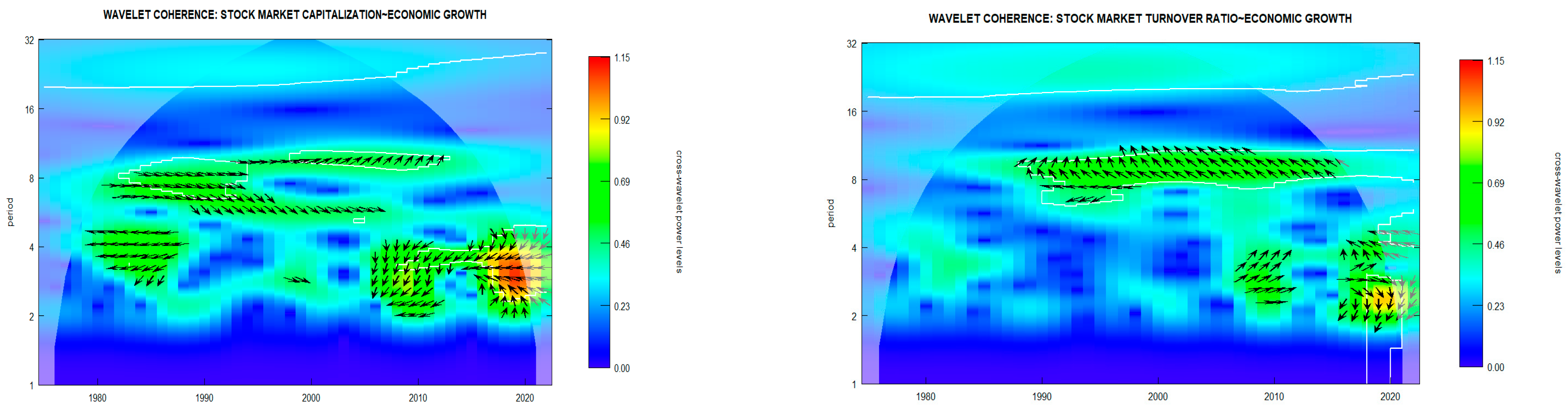
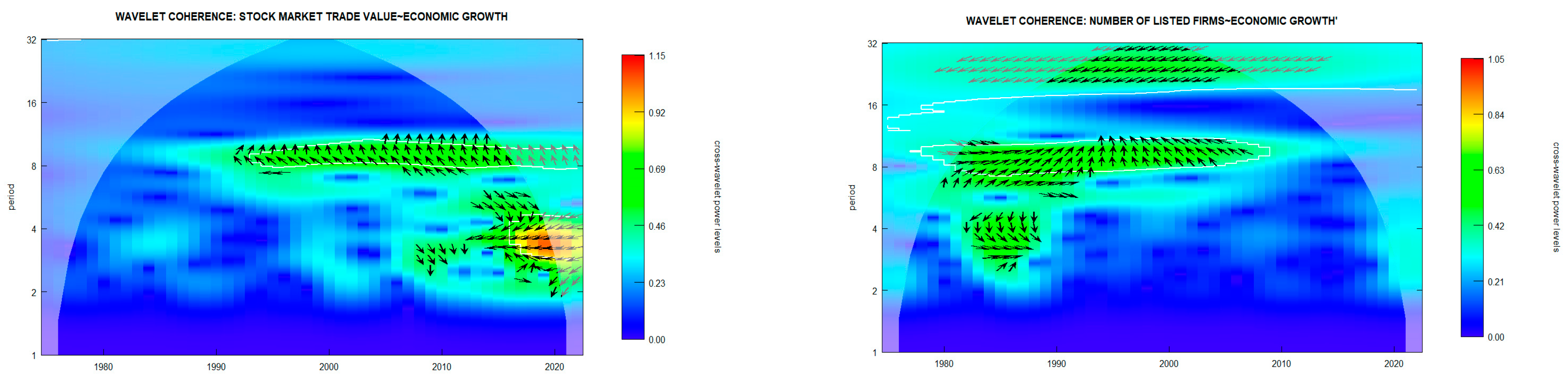
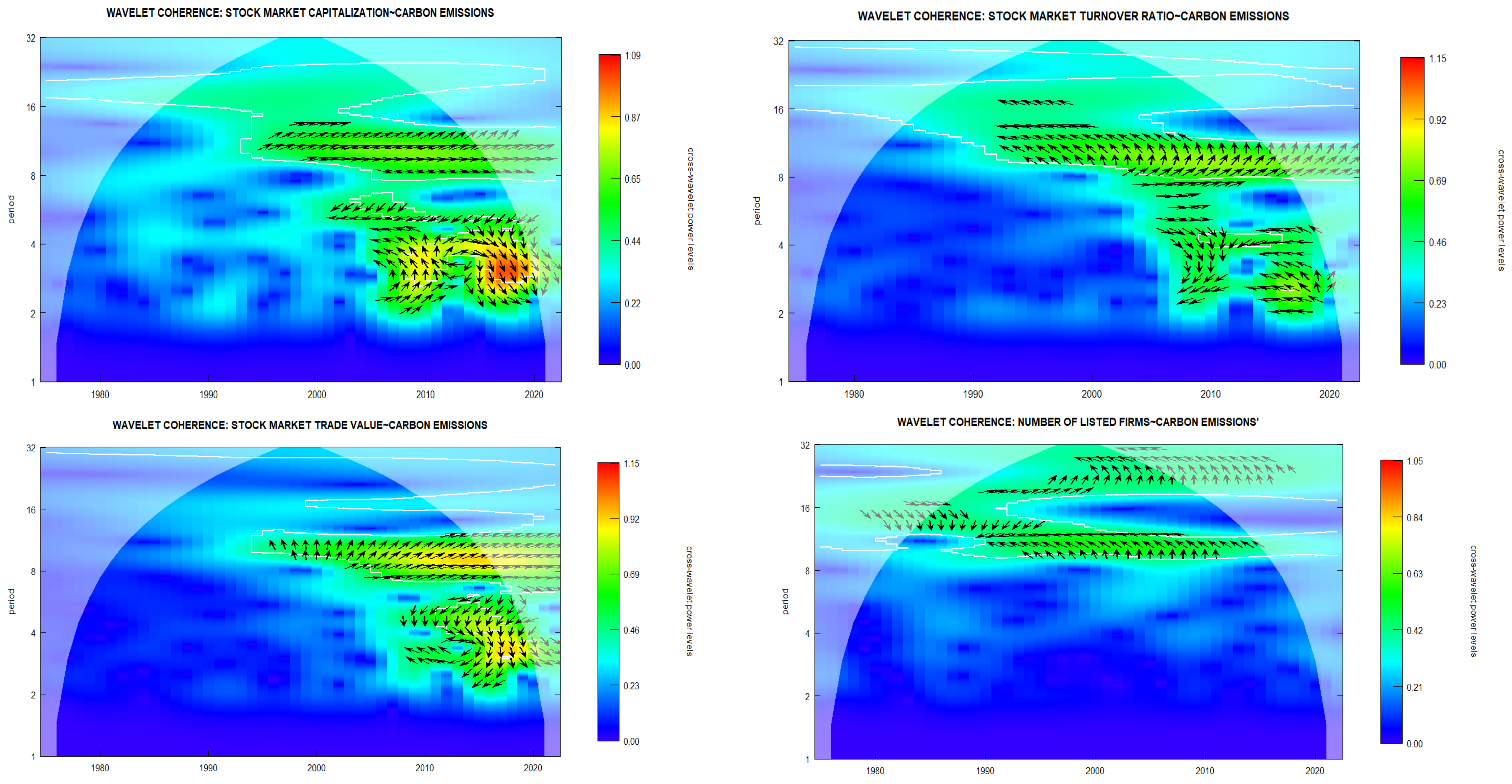
We now present the wavelet coherence results via heat-map plots (Figure 4 and Figure 5) showing time–frequency correlations between stock market indicators and economic growth/carbon emissions. The horizontal axis denotes time and the vertical axis frequency (scale), and color contours reflect correlation strength—cooler colors indicate weaker, warmer stronger relationships. Arrows within these contours reveal phase dynamics: the arrow direction indicates the sign of co-movement (↑, → = positive; ↓, ← = negative) and lead–lag patterns (e.g., → means stock market leads, and ← means lags). Note that in all wavelet plots, significant coherence appears in both long-term (8–32-year cycles) and short-term (0–4-year cycles) frequencies.

For stock market–growth (Figure 4), long-term co-movements show: (i) capitalization is positively correlated with growth throughout the sample; (ii) turnover and trade value exhibit negative co-movement post-1990; and (iii) the number of firms shows positive coherence in 1980–2000 (8–16-year cycles), turning negative in 1990–2022 (16–32-year cycles). At higher frequencies, all stock variables display negative co-movement with growth during crisis periods—the 2008 financial crisis, 2016 EM sell-off, and 2020 COVID-19.

For stock market–emissions (Figure 5), at low frequencies: (i) capitalization and trade value exhibit positive co-movement since the early 1990s; (ii) turnover shows a negative relationship from 1990 to 2010, which then turns positive; and (iii) the number of firms displays a shift from positive to negative co-movement. At short-term cycles, emission relationships are largely negative, again concentrated around major global crises. Summaries of the phase dynamics and durations of significant coherence described from Figure 4 and Figure 5 are reported in

Table 5. Summary of wavelet coherency between stock market development and economic growth.

Function	8–32-Year Cycles			0–4 Year-Cycles
	Period	Sign	Lead/Lag	Period	Sign	Lead/Lag
f(GDP~MCR)	1980–2010	+ve	stock→gdp	2008–2012	−ve	stock→gdp
	N/A	N/A	N/A	2016–2020	−ve	stock→gdp
f(GDP~TURNOVER)	1990–2020	−ve	gdp→stock	2016–2022	−ve	stock→gdp
f(GDP~VALUE)	1990–2022	−ve	stock→gdp	2016–2020	−ve	stock→gdp
f(GDP~NUMBER)	1980–2000	+ve	gdp→stock	N/A	N/A	N/A
	1980–2022	−ve	gdp→stock	N/A	N/A	N/A

and

Table 6. Summary of wavelet coherency between stock market development and carbon emissions.

Function	8–16-Year Cycles			0–4-Year Cycles
	Period	Sign	Lead/Lag	Period	Sign	Lead/Lag
f(CO2~MCR)	1990–2022	+ve	stock→CO	2007–2009	−ve	stock→CO
	N/A	N/A	N/A	2016–2020	+ve	stock→CO
f(CO2~TURNOVER)	1990–2010	−ve	CO→stock	2016–2022	−ve	stock→CO
	2010–2022	+ve	stock→CO	N/A	N/A	N/A
f(CO2~VALUE)	1994–2022	+ve	stock→CO	2016–2020	−ve	stock→CO
f(CO2~NUMBER)	1980–2000	+ve	stock→CO	N/A	N/A	N/A
	2000–2022	−ve	stock→CO	N/A	N/A	N/A

, respectively.

5. Discussion of Results

In this section, we provide further discussions of our empirical results. Firstly, we contextualize our findings in light of the previous related South Africa literature. Secondly, we derive policy implications associated with our empirical findings.

5.1. Comparison to the Previous Literature

The ARDL results reveal that the negative or insignificant relationship between stock market development (SMD) and economic growth aligns with prior country-specific (Nyasha & Odhiambo, 2015) and panel-based studies (Adjasi & Biekpe, 2006; Enisan & Olufisayo, 2009; Yu et al., 2012; Rioja & Valev, 2014; Fufa & Kim, 2018; Pradhan et al., 2020). In contrast, the similarly negative or insignificant SMD–emission link challenges the existing literature, which typically finds a positive connection (Paramati et al., 2017; Jiang & Ma, 2019; Habiba et al., 2021; Mhadhbi et al., 2021; R. Zhang et al., 2022). Notably, nonlinear (kinked) ARDL models indicate that both positive and negative effects of SMD on growth and emissions can coexist (i.e., depending on the level of market development), with positive impacts emerging only at more advanced stages.

Wavelet coherence analysis further reveals time-varying dynamics. Before 1990, only market size and breadth (capitalization and number of firms) supported growth but also harmed the environment, while depth (liquidity and activity) had no discernible impact. These patterns reflect three strands in the literature: studies showing positive SMD–growth effects (e.g., Rousseau & Wachtel, 2000; Durham, 2002; Beck & Levine, 2004; Ndako, 2010; Khetsi & Mongale, 2014; Phiri, 2015; Ananwude & Osakwe, 2017; Fapohunda, 2019; Osakwe et al., 2020), those reporting insignificant effects (Adjasi & Biekpe, 2006; Enisan & Olufisayo, 2009; Yu et al., 2012; Rioja & Valev, 2014; Fufa & Kim, 2018; Pradhan et al., 2020), and those confirming positive effects on emissions (Paramati et al., 2017; Jiang & Ma, 2019; Habiba et al., 2021; Mhadhbi et al., 2021; R. Zhang et al., 2022). Post-1994, with South Africa’s reintegration and JSE expansion, depth indicators began significantly influencing both growth and emissions, while the number of listed firms showed a negative link with emissions. During crises, SMD displayed short-term negative co-movements with both growth and carbon emissions, and this is line with the findings of Ogbeide and Akanji (2018) for BRICS economies during the global financial crisis. However, the negative SMD–emission relationship observed for South Africa is novel to the previous South African-based literature and is consistent with the findings of Akinlo and Apanisile (2023) for Nigeria.

5.2. Policy Implications of Findings

The key policy insight from our analysis is that the Johannesburg Stock Exchange (JSE) currently cannot foster economic growth and environmental sustainability simultaneously. While post-apartheid structural reforms expanded market size and depth and breadth contributed positively to growth, it also exacerbated carbon emissions. Conversely, tighter regulatory and compliance standards post-2000, reflected in the delisting wave, helped reduce emissions and support growth, albeit at the expense of market breadth—an important component for diversification (Yartey & Adjasi, 2007). Importantly, the emission reductions observed during crisis periods stem from economic slowdowns and reduced stock market activity and are therefore temporary.

To sustainably align financial development with environmental goals, policymakers must move beyond restricting ‘dirty’ firms and adopt structural strategies that ‘green’ the market without impeding growth. One promising avenue is enhancing stock market depth. This can include promoting institutional investments in clean technology, renewable energy, and low-carbon firms, as well as developing green trading platforms and incentivizing ESG-compliant market participants. Such targeted measures can redirect liquidity and trading activity toward environmentally responsible sectors, helping reshape the JSE into a platform that supports both economic and ecological progress.

6. Conclusions and Policy Implications

We investigate the dual role of stock market development (SMD) in driving economic growth and influencing environmental outcomes in South Africa from 1975 to 2022 by using ARDL models and wavelet coherence analysis. We find that initially, stock market development, particularly in terms of size and breadth, supported economic growth but simultaneously contributed to environmental degradation. In contrast, stock market depth (liquidity and trading activity) showed no significant impact on economic growth or environmental degradation before the 1990s but gained importance following South Africa’s democratic transition and deeper integration into the global economy. Our findings also highlight a critical distinction: while stock market expansion can enhance growth, its environmental cost is not linear and depends on the specific dimensions of development.

A key insight from our analysis is that the decline in the number of JSE-listed ordinary equity companies, particularly from the early 2000s onward, coincided with an improvement in environmental outcomes without eliminating the growth potential of the stock market. This period was characterized by a substantial reduction in the number of listed companies, with delistings outnumbering new listings and the JSE subsequently becoming more concentrated among larger firms. The decline in listings reflects corporate consolidation, liquidation, weak market conditions, and the costs and benefits of remaining publicly listed. Our findings therefore suggest an important trade-off: reducing the breadth of the equity market may be associated with lower carbon emissions, but it may also limit diversification and access to equity finance. Rather than encouraging further delistings, policy should seek to preserve market breadth while improving the environmental composition of listed firms through stronger climate-related disclosure, ESG standards, and incentives for low-carbon investment.

In light of these findings, we argue that future policy should move beyond reactive measures aimed solely at controlling the number of high-emission firms. Instead, structural reforms are needed to integrate environmental objectives into the fabric of stock market development. This involves ‘greening’ the liquidity and activity dimensions of the market by incentivizing capital flows toward clean energy and low-carbon sectors. By fostering green trading platforms and supporting ESG-aligned institutional investors, South Africa’s policymakers can reshape the JSE into a lever for sustainable growth which does not force a choice between economic progress and environmental responsibility but rather aligns the two in a mutually reinforcing trajectory.

Limitations and Avenues for Future Research

Notwithstanding these contributions, several limitations should be acknowledged. Firstly, our analysis is confined to a single-country case study. While this allows for a deeper understanding of country-specific dynamics, it limits the generalizability of the findings to other emerging or African markets with different institutional, regulatory, and energy structures. Secondly, although the ARDL and wavelet coherence frameworks capture nonlinearities and time–frequency dynamics, they remain reduced-form approaches and do not explicitly model structural transmission channels (e.g., sectoral reallocation, technological adoption, or green innovation mechanisms). Thirdly, our environmental proxy is limited to aggregate CO₂ emissions, which may mask sectoral heterogeneity and overlook other dimensions of environmental sustainability such as energy efficiency, renewable energy penetration, or broader ecological indicators. Fourthly, while we control for standard macroeconomic factors, potential endogeneity and omitted variable bias cannot be entirely ruled out, particularly given the complex two-way interactions between financial development, growth, and environmental performance.

These limitations open several promising avenues for future research. Firstly, extending the analysis to a comparative multi-country framework, particularly across African or BRICS economies, would help assess whether the nonlinear and time-varying dynamics identified for South Africa are structurally generalizable or institution-specific. Secondly, future studies could incorporate sector-level emission data to examine whether stock market development reallocates capital toward cleaner industries or merely shifts pollution intensity within sectors. Thirdly, micro-level or firm-level analyses could provide insights into how listing status, ESG compliance, and governance reforms influence environmental performance and productivity outcomes. Fourthly, structural or dynamic stochastic general equilibrium (DSGE) models incorporating financial frictions and environmental externalities could offer deeper theoretical grounding for the observed nonlinearities. Lastly, given the growing relevance of sustainable finance instruments, future work could explicitly evaluate the role of green bonds, ESG indices, and climate-related disclosure regulations in reshaping the growth–emission trade-off.

References

1. Acheampong, A. O., Amponsah, M., & Boateng, E. (2020). Does financial development mitigate carbon emissions? Evidence from heterogeneous financial economies. Energy Economics, 88, 104768. [Google Scholar] [CrossRef] [Scilit]
2. Adjasi, C. K., & Biekpe, N. B. (2006). Stock market development and economic growth: The case of selected African countries. African Development Review, 18(1), 144–161. [Google Scholar] [CrossRef] [Scilit]
3. Aguiar-Conraria, L., & Soares, M. J. (2011). Oil and the macroeconomy: Using wavelets to analyze old issues. Empirical Economics, 40(3), 645–655. [Google Scholar] [CrossRef] [Scilit]
4. Aguiar-Conraria, L., & Soares, M. J. (2014). The continuous wavelet transform: Moving beyond uni-and bivariate analysis. Journal of Economic Surveys, 28(2), 344–375. [Google Scholar] [CrossRef] [Scilit]
5. Akinlo, A. E., & Apanisile, O. (2023). Stock markets and carbon emissions nexus in Nigeria: Evidence from nonlinear ARDL and causality approaches. Energy and Climate Change, 4, 100091. [Google Scholar] [CrossRef] [Scilit]
6. Ananwude, A. C., & Osakwe, C. I. (2017). Stock market development and economic growth: A comparative evidence from two emerging economies in Africa: Nigeria and South Africa. Archives of Current Research International, 11(1), 1–15. [Google Scholar] [CrossRef] [Scilit][Green Version]
7. Ang, J. B. (2008). A survey of recent developments in the literature of finance and growth. Journal of Economic Surveys, 22(3), 536–576. [Google Scholar] [CrossRef] [Scilit]
8. Arestis, P., Demetriades, P. O., & Luintel, K. B. (2001). Financial development and economic growth: The role of stock markets. Journal of Money, Credit and Banking, 33, 16–41. [Google Scholar] [CrossRef] [Scilit]
9. Banerjee, A., Dolado, J., & Mestre, R. (1998). Error-correction mechanism tests for cointegration in a single-equation framework. Journal of Time Series Analysis, 19(3), 267–283. [Google Scholar] [CrossRef] [Scilit]
10. Beck, T., & Levine, R. (2004). Stock markets, banks, and growth: Panel evidence. Journal of Banking & Finance, 28(3), 423–442. [Google Scholar] [CrossRef] [Scilit]
11. Bencivenga, V. R., Smith, B. D., & Starr, R. M. (1996). Liquidity of secondary capital markets: Allocative efficiency and the maturity composition of the capital stock. Economic Theory, 7(1), 19–50. [Google Scholar] [CrossRef] [Scilit]
12. Boyd, J. H., & Smith, B. D. (1998). The evolution of debt and equity markets in economic development. Economic Theory, 12, 519–560. [Google Scholar] [CrossRef] [Scilit]
13. Cave, J., Chaudhuri, K., & Kumbhakar, S. C. (2020). Do banking sector and stock market development matter for economic growth? Empirical Economics, 59(4), 1513–1535. [Google Scholar] [CrossRef] [Scilit]
14. Damasceno, A. O., & Guedes, D. R. (2024). Financial openness, capital accumulation, and productivity in emerging and developing economies. Economic Modelling, 133, 106663. [Google Scholar] [CrossRef] [Scilit]
15. De Beer, J., Keyser, N., & Van der Merwe, I. (2015). The Johannesburg stock exchange (JSE) returns, political development and economic forces: A historical perspective. Journal for Contemporary History, 40(2), 1–24. [Google Scholar] [CrossRef] [Scilit]
16. Durham, J. B. (2002). The effects of stock market development on growth and private investment in lower-income countries. Emerging Markets Review, 3(3), 211–232. [Google Scholar] [CrossRef] [Scilit]
17. Enisan, A. A., & Olufisayo, A. O. (2009). Stock market development and economic growth: Evidence from seven sub-Sahara African countries. Journal of Economics and Business, 61(2), 162–171. [Google Scholar] [CrossRef] [Scilit]
18. Fapohunda, F. M. (2019). Stock market development and economic growth in Nigeria and South Africa: Comparative empirical analysis. Accounting and Taxation Review, 3(1), 93–104. [Google Scholar]
19. Fufa, T., & Kim, J. (2018). Stock markets, banks, and economic growth: Evidence from more homogeneous panels. Research in International Business and Finance, 44, 504–517. [Google Scholar] [CrossRef] [Scilit]
20. Ganda, F. (2018). The effect of carbon performance on corporate financial performance in a growing economy. Social Responsibility Journal, 14(4), 895–916. [Google Scholar] [CrossRef] [Scilit]
21. Greenwood, J., & Smith, B. D. (1997). Financial markets in development, and the development of financial markets. Journal of Economic Dynamics and Control, 21(1), 145–181. [Google Scholar] [CrossRef] [Scilit]
22. Grossman, G. M., & Krueger, A. B. (1991). Environmental impacts of a North American free trade agreement (NBER working paper no. 3914). National Bureau of Economic Research. [Google Scholar]
23. Grossman, G. M., & Krueger, A. B. (1993). Economic development and the Environment. The Quarterly Journal of Economics, 110(2), 353–377. [Google Scholar]
24. Ha, L. T. (2022). Financial development and renewable energy consumption in Vietnam: Evidence from a wavelet approach. Environment, Development and Sustainability, 27, 20861–20885. [Google Scholar] [CrossRef] [Scilit]
25. Ha, N. M., Hoang Ngoc, B., & Vo, D. H. (2023). Does financial development affect human capital? Evidence from Vietnam. Journal of Asia Business Studies, 17(4), 785–803. [Google Scholar] [CrossRef] [Scilit]
26. Habiba, U., Xinbang, C., & Ahmad, R. I. (2021). The influence of stock market and financial institution development on carbon emissions with the importance of renewable energy consumption and foreign direct investment in G20 countries. Environmental Science and Pollution Research, 28, 67677–67688. [Google Scholar] [CrossRef] [Scilit] [PubMed]
27. Hung, N. T. (2023). Green investment, financial development, digitalization and economic sustainability in Vietnam: Evidence from a quantile-on-quantile regression and wavelet coherence. Technological Forecasting and Social Change, 186, 122185. [Google Scholar] [CrossRef] [Scilit]
28. Jalloh, M. (2015). Does stock market capitalization influences economic growth in Africa? Evidence from panel data. Applied Economics and Finance, 2(1), 91–101. [Google Scholar] [CrossRef] [Scilit][Green Version]
29. Jiang, C., & Ma, X. (2019). The impact of financial development on carbon emissions: A global perspective. Sustainability, 11(19), 5241. [Google Scholar] [CrossRef] [Scilit]
30. Keyser, N., Van der Merwe, I., & De Beer, J. (2020). The Johannesburg stock exchange returns, political developments and economic forces: A historical perspective of the 1990s. New Contree, 84, 20. [Google Scholar] [CrossRef] [Scilit]
31. Khetsi, Q. S., & Mongale, I. P. (2014). The impact of capital markets on the economic growth in South Africa. Journal of Governance and Regulation, 3(2), 154–163. [Google Scholar] [CrossRef] [Scilit]
32. Lau, K. M., & Weng, H. (1995). Climate signal detection using wavelet transform: How to make a time series sing. Bulletin of the American Meteorological Society, 76(12), 2391–2402. [Google Scholar] [CrossRef] [Scilit]
33. Levine, R. (1991). Stock markets, growth, and tax policy. The Journal of Finance, 46(4), 1445–1465. [Google Scholar] [CrossRef]
34. Levine, R. (1997). Financial development and economic growth: Views and agenda. Journal of Economic Literature, 35(2), 688–726. [Google Scholar]
35. Levine, R., & Zervos, S. (1998). Stock markets, banks, and economic growth. American Economic Review, 88, 537–558. [Google Scholar]
36. Masten, A. B., Coricelli, F., & Masten, I. (2008). Non-linear growth effects of financial development: Does financial integration matter? Journal of International Money and Finance, 27(2), 295–313. [Google Scholar] [CrossRef] [Scilit]
37. Mhadhbi, M., Gallali, M. I., Goutte, S., & Guesmi, K. (2021). On the asymmetric relationship between stock market development, energy efficiency and environmental quality: A nonlinear analysis. International Review of Financial Analysis, 77, 101840. [Google Scholar] [CrossRef] [Scilit]
38. Mkhize, H., & Msweli-Mbanga, P. (2006). A critical review of the restructuring of the South African capital market. International Review of Business Research Papers, 2(2), 80–91. [Google Scholar]
39. Morlet, J., Arens, G., Fourgeau, E., & Giard, D. (1982a). Wave propagation and sampling theory; Part I, Complex signal and scattering in multilayered media. Geophysics, 47(2), 203–221. [Google Scholar] [CrossRef] [Scilit]
40. Morlet, J., Arens, G., Fourgeau, E., & Giard, D. (1982b). Wave propagation and sampling theory—Part II: Sampling theory and complex waves. Geophysics, 47(2), 222–236. [Google Scholar] [CrossRef] [Scilit]
41. Narayan, P. K. (2004). Fiji’s tourism demand: The ARDL approach to cointegration. Tourism Economics, 10(2), 193–206. [Google Scholar] [CrossRef] [Scilit]
42. Ndako, U. B. (2010). Stock markets, banks and economic growth: Time series evidence from South Africa. African Finance Journal, 12(2), 72–92. [Google Scholar]
43. Ngare, E., Nyamongo, E. M., & Misati, R. N. (2014). Stock market development and economic growth in Africa. Journal of Economics and Business, 74, 24–39. [Google Scholar] [CrossRef] [Scilit]
44. Nyasha, S., & Odhiambo, N. M. (2015). The impact of banks and stock market development on economic growth in South Africa: An ARDL-bounds testing approach. Contemporary Economics, 9(1), 93–108. [Google Scholar] [CrossRef] [Scilit]
45. Ogbeide, S., & Akanji, B. (2018). Stock market development and economic growth of Brazil, Russia, India, China and South African (BRICS) Nations: An empirical research. Accounting, 4(2), 83–92. [Google Scholar] [CrossRef] [Scilit]
46. Osakwe, C. I., Ogbonna, K. S., & Obi-Nwosu, V. O. (2020). Stock Market capitalization and economic growth of Nigeria and South Africa (2000–2018). European Academic Research Journal, 7(11), 5605–5623. [Google Scholar]
47. Paramati, S. R., Mo, D., & Gupta, R. (2017). The effects of stock market growth and renewable energy use on CO2 emissions: Evidence from G20 countries. Energy Economics, 66, 360–371. [Google Scholar] [CrossRef] [Scilit]
48. Pask, A. (2024). Can the JSE stem the tide of delistings, and what does this mean for SA investors? MoneyMarketing, 2024(8), 6. [Google Scholar]
49. Pesaran, M. H., Shin, Y., & Smith, R. J. (2001). Bounds testing approaches to the analysis of level relationships. Journal of Applied Econometrics, 16(3), 289–326. [Google Scholar] [CrossRef] [Scilit]
50. Phiri, A. (2015). Asymmetric cointegration and causality effects between financial development and economic growth in South Africa. Studies in Economics and Finance, 32(4), 464–484. [Google Scholar] [CrossRef] [Scilit]
51. Phiri, A. (2020). Structural changes in exchange rate-stock returns dynamics in South Africa: Examining the role of crisis and new trading platform. Economic Change and Restructuring, 53(1), 171–193. [Google Scholar] [CrossRef] [Scilit]
52. Phiri, A., Mhaka, S., & Taonezvi, L. (2024). Too poor to be clean? A quantile ARDL assessment of the environmental Kuznets curve in SADC countries. Environment, Development and Sustainability, 26(11), 27301–27323. [Google Scholar] [CrossRef] [Scilit]
53. Phiri, A., & Nyoni, B. (2023). Clean versus dirty electricity generation and economic growth in South Africa: Time–frequency study. Economic Change and Restructuring, 56(4), 2801–2824. [Google Scholar] [CrossRef] [Scilit]
54. Pradhan, R. P., Arvin, M. B., Norman, N. R., & Bahmani, S. (2020). The dynamics of bond market development, stock market development and economic growth: Evidence from the G-20 countries. Journal of Economics, Finance and Administrative Science, 25(49), 119–147. [Google Scholar]
55. Rioja, F., & Valev, N. (2014). Stock markets, banks and the sources of economic growth in low and high income countries. Journal of Economics and Finance, 38, 302–320. [Google Scholar] [CrossRef] [Scilit]
56. Rousseau, P. L., & Wachtel, P. (2000). Equity markets and growth: Cross-country evidence on timing and outcomes, 1980–1995. Journal of Banking & Finance, 24(12), 1933–1957. [Google Scholar] [CrossRef] [Scilit]
57. Shahbaz, M., Tiwari, A. K., & Nasir, M. (2013). The effects of financial development, economic growth, coal consumption and trade openness on CO2 emissions in South Africa. Energy Policy, 61, 1452–1459. [Google Scholar] [CrossRef] [Scilit]
58. Sharma, R., Shahbaz, M., Sinha, A., & Vo, X. V. (2021). Examining the temporal impact of stock market development on carbon intensity: Evidence from South Asian countries. Journal of Environmental Management, 297, 113248. [Google Scholar] [CrossRef] [Scilit] [PubMed]
59. Stern, D. I. (2004). The rise and fall of the environmental Kuznets curve. World Development, 32(8), 1419–1439. [Google Scholar] [CrossRef] [Scilit]
60. Subhan, M., Irfan, M., Ahmad, G., Alam, W., & Zameer, M. N. (2023). Modelling the asymmetric effects of renewable and nonrenewable energy consumption and financial development on CO2 emissions in India: Empirical findings from the NARDL and wavelet coherence approach. Environmental Science and Pollution Research, 30(34), 82264–82285. [Google Scholar] [CrossRef] [Scilit] [PubMed]
61. Tamazian, A., Chousa, J. P., & Vadlamannati, K. C. (2009). Does higher economic and financial development lead to environmental degradation: Evidence from BRIC countries. Energy Policy, 37(1), 246–253. [Google Scholar] [CrossRef] [Scilit]
62. Tan, Y., Lin, B., & Wang, L. (2025). Green finance and corporate environmental performance. International Review of Economics & Finance, 98, 103929. [Google Scholar] [CrossRef] [Scilit]
63. Thaddeus, K. J., Ngong, C. A., Nnecka, U. J., Nubong, N. M., Ibe, G. I., Chinyere C, O., & Onwumere, J. U. J. (2024). Stock market development and economic growth in sub-Saharan Africa (1990–2020): An ARDL approach. Journal of Economic and Administrative Sciences, 40(2), 344–363. [Google Scholar] [CrossRef] [Scilit]
64. Torrence, C., & Compo, G. P. (1998). A practical guide to wavelet analysis. Bulletin of the American Meteorological society, 79(1), 61–78. [Google Scholar] [CrossRef] [Scilit]
65. Yartey, C. A., & Adjasi, C. K. (2007). Stock market development in Sub-Saharan Africa: Critical issues and challenges. International Monetary Fund. [Google Scholar]
66. Yu, J. S., Hassan, M. K., & Sanchez, B. (2012). A re-examination of financial development, stock markets development and economic growth. Applied Economics, 44(27), 3479–3489. [Google Scholar] [CrossRef] [Scilit]
67. Zafar, M. W., Zaidi, S. A. H., Sinha, A., Gedikli, A., & Hou, F. (2019). The role of stock market and banking sector development, and renewable energy consumption in carbon emissions: Insights from G-7 and N-11 countries. Resources Policy, 62, 427–436. [Google Scholar] [CrossRef] [Scilit]
68. Zeqiraj, V., Sohag, K., & Soytas, U. (2020). Stock market development and low-carbon economy: The role of innovation and renewable energy. Energy Economics, 91, 104908. [Google Scholar] [CrossRef] [Scilit]
69. Zhang, R., Sharma, R., Tan, Z., & Kautish, P. (2022). Do export diversification and stock market development drive carbon intensity? The role of renewable energy solutions in top carbon emitter countries. Renewable Energy, 185, 1318–1328. [Google Scholar] [CrossRef] [Scilit]
70. Zhang, Y. J. (2011). The impact of financial development on carbon emissions: An empirical analysis in China. Energy Policy, 39(4), 2197–2203. [Google Scholar] [CrossRef] [Scilit]
71. Zhao, B., & Yang, W. (2020). Does financial development influence CO2 emissions? A Chinese province-level study. Energy, 200, 117523. [Google Scholar] [CrossRef] [Scilit]
Figure 1. Time series evolution of GDP growth, CO2 emissions and stock market development.
Economies 14 00472 g001
Figure 2. Correlations between stock market development and GDP growth.
Economies 14 00472 g002
Figure 3. Correlations between stock market development and CO2 emissions.
Economies 14 00472 g003
Figure 4. Wavelet coherence plots for stock market activity–economic growth correlations. Note: The horizontal axis shows time, and the vertical axis shows frequency (period). Colors indicate wavelet coherence from low (blue) to high (red). Black arrows show the direction and lead–lag relationship between stock market capitalization and economic growth. White contours indicate significance at the 5% level, and the shaded cone marks areas affected by edge effects.
Economies 14 00472 g004aEconomies 14 00472 g004b
Figure 5. Wavelet coherence plots for stock market activity–carbon emissions. Note: The horizontal axis shows time, and the vertical axis shows frequency (period). Colors indicate wavelet coherence from low (blue) to high (red). Black arrows show the direction and lead–lag relationship between stock market capitalization and carbon emissions. White contours indicate significance at the 5% level, and the shaded cone marks areas affected by edge effects.
Economies 14 00472 g005