Does Financial Development Affect Economic Growth Asymmetrically in Algeria? Evidence from a PCA-Based NARDL Model

Abstract

This study examines whether financial development affects economic growth asymmetrically in Algeria using annual data for 1980–2020. Algeria represents a particularly relevant case because its hydrocarbon dependence, bank-based financial system, strong state involvement in banking, and exposure to oil-price and macroeconomic shocks may shape the finance–growth relationship differently from more diversified economies. The study constructs a composite financial development index using principal component analysis of liquid liabilities, private-sector credit, and bank deposits to GDP (%); the first component explains 81.25% of total variance. A nonlinear autoregressive distributed lag (NARDL) model is estimated with trade openness and government expenditure as controls. Unit-root tests confirm that the variables are I(0) or I(1), and the bounds test supports cointegration (F = 7.455). In the long run, trade openness positively affects growth, whereas government expenditure is statistically insignificant. Positive financial-development shocks are associated with lower long-run growth, although the coefficient is significant only at the 10% level, while negative shocks are insignificant. In the short run, positive shocks generate delayed growth benefits after one and two years. Although the Wald test rejects long-run symmetry within the estimated specification, uncertainty around the individual long-run coefficients warrants interpreting the findings as suggestive evidence of asymmetry that requires further confirmation. Short-run symmetry is not rejected. The error-correction coefficient (−0.674) implies rapid adjustment toward equilibrium. The findings suggest that the quality and productive allocation of financial resources may matter more for growth than financial deepening alone.

1. Introduction

Financial development can promote growth by mobilizing savings, evaluating borrowers, diversifying risk, and directing funds toward productive investment (Beck et al., 2000; Levine, 2005). Nevertheless, financial depth does not necessarily imply efficient intermediation. Credit and liquidity expansion may support productive firms but may also finance consumption, speculative activity, or low-return projects, producing nonlinear or even adverse growth effects (Arcand et al., 2015; Ductor & Grechyna, 2015; Law & Singh, 2014). The central research problem is therefore whether increases and decreases in financial development affect economic growth differently in the short and long run.

This question is particularly relevant to Algeria, a hydrocarbon-dependent, bank-based economy exposed to oil-price shocks, structural reforms, and macroeconomic instability. The strong state presence in banking makes governance, regulation, and credit allocation especially important (Al Khatib et al., 2023; Hadfi et al., 2026). Evidence from another oil-rich economy indicates that financial development can benefit non-oil activity while having insignificant or negative effects on aggregate growth, demonstrating how resource dependence may alter the finance–growth relationship (Samargandi et al., 2014).

Previous research provides no consensus on the finance–growth relationship. Early studies generally emphasize the growth-enhancing role of financial development, whereas subsequent evidence identifies nonlinearities, diminishing returns, and threshold effects (Ang & McKibbin, 2007; Arcand et al., 2015; Ductor & Grechyna, 2015; Law & Singh, 2014). More recent studies further show that the estimated relationship is sensitive to the measure of financial development, institutional conditions, and empirical specification (Botev et al., 2019; Luintel et al., 2024; Nguyen et al., 2022). The asymmetric literature likewise reports mixed results. Chen et al. (2020) identify different short- and long-run responses to positive and negative financial-development shocks in Kenya, while Appiah et al. (2026) find short-run but not long-run asymmetry in Ghana. For Algeria, Al Khatib et al. (2023) report symmetric effects using an IMF financial-development index. These contrasting findings leave it unclear whether alternative measures of financial development and asymmetric specifications yield different conclusions for Algeria.

This study matters because a symmetric linear coefficient may conceal policy-relevant differences between financial expansion and contraction, potentially leading to inappropriate financial-sector policies.

The study aims to evaluate the asymmetric short- and long-run effects of financial development on Algerian economic growth during 1980–2020. It constructs a PCA-based index from liquid liabilities, private-sector credit, and bank deposits to GDP (%); investigates stationarity and structural breaks; tests cointegration; estimates positive and negative financial shocks while controlling for trade openness and government expenditure; and evaluates model adequacy. The analysis applies the bounds-testing and NARDL frameworks of Pesaran et al. (2001) and Shin et al. (2014).

Against this background, this study examines whether positive and negative changes in financial development have different short- and long-run associations with economic growth in Algeria from 1980 to 2020. Financial development is represented by a composite index constructed through principal component analysis (PCA) from liquid liabilities, private-sector credit, and bank deposits, measured as a share of GDP. We also include trade openness and government expenditure as controls. The empirical analysis applies the nonlinear autoregressive distributed lag (NARDL) framework of Shin et al. (2014), together with unit-root and structural-break tests, bounds cointegration testing, Wald symmetry restrictions, and model-stability diagnostics. The analysis addresses whether a long-run relationship exists, whether financial expansions and contractions generate asymmetric long- or short-run responses, and how rapidly deviations from equilibrium are corrected.

This study makes three contributions to the existing literature. First, it provides new country-specific evidence on the finance–growth nexus in Algeria by explicitly distinguishing positive and negative financial-development changes, thereby extending previous Algeria-specific evidence based on symmetric or alternative financial-development measures. Second, rather than relying on a single financial proxy, the study constructs a PCA-based composite index from three indicators of financial depth, reducing dependence on any single measure and allowing the analysis to capture their common variation. Third, the study combines this composite measure with an NARDL framework and complementary structural-break, cointegration, symmetry, and stability tests, providing an integrated assessment of both the direction and the time horizon of the finance–growth relationship.

The empirical results indicate a stable long-run relationship among economic growth, financial development, trade openness, and government expenditure. The Wald test rejects long-run symmetry within the estimated specification; however, because the individual long-run financial-development coefficients are not significant at the 5% level, this evidence is interpreted as suggestive rather than conclusive. Positive financial-development shocks are associated with a negative long-run coefficient that is significant only at the 10% level, whereas the corresponding coefficient for negative shocks is statistically insignificant. In the short run, positive financial-development shocks generate significant delayed positive effects after one and two years, although the Wald test does not reject overall short-run symmetry. Trade openness is positively associated with growth in the long run, government expenditure is statistically insignificant, and the negative error-correction coefficient indicates relatively rapid adjustment toward long-run equilibrium.

The remainder of the paper is organized as follows. Section 2 reviews the theoretical and empirical literature, identifies the research gap, and develops the study hypotheses. Section 3 describes the data, construction of the PCA-based financial-development index, and econometric methodology. Section 4 presents the empirical results and diagnostic analyses. Section 5 discusses the findings in relation to previous evidence and the Algerian context. Section 6 concludes with the main findings, policy considerations, limitations, and directions for future research.

2. Literature Review

2.1. Theoretical Background

Supply-leading theory holds that finance promotes growth by mobilizing savings, screening investment, monitoring borrowers, and sharing risk, whereas demand-following theory views financial development as a response to real-sector expansion (Levine, 2005). Feedback theory combines both directions. Nonlinear models add that finance may provide limited benefits below a minimum scale or set of institutional conditions and diminishing returns after excessive expansion (Deidda & Fattouh, 2002). Trade openness can foster specialization and technology diffusion (Frankel & Romer, 1999), while productive public spending can support demand, infrastructure, and human capital (Devarajan et al., 1996). These competing mechanisms justify jointly examining finance, trade, government expenditure, and growth within a dynamic asymmetric framework.

2.2. Financial Development and Economic Growth

Evidence from leading journals provides substantial support for a growth role of financial development, while also showing that the relationship is conditional rather than universally linear. Levine et al. (2000), using instrumental-variable and dynamic-panel methods, find that the exogenous component of financial-intermediary development is positively associated with economic growth. Aghion et al. (2005) further show that financial development affects countries’ ability to converge toward the world technology frontier. However, subsequent evidence emphasizes important institutional and structural contingencies. Law et al. (2013) identify an institutional-quality threshold, showing that financial development supports growth only after a sufficient level of institutional development. Beck et al. (2014) similarly distinguish financial intermediation from overall financial-sector size, finding that intermediation activities support long-run growth whereas broader financial-sector expansion does not necessarily do so.

The direction and strength of the relationship also depend on how financial development is measured and on the prevailing macroeconomic environment. Peia and Roszbach (2015) find that causality patterns differ between banking-sector and stock-market development, while Asteriou et al. (2024) show that the finance–growth relationship varies between normal and stress periods and across measures of financial depth, access, and efficiency. These findings complement evidence that credit quality, institutional conditions, and banking efficiency influence the growth effects of finance (Demetriades & Rewilak, 2020; Bayraktar et al., 2023; Xu, 2025). Overall, the literature supports a multidimensional approach to financial development and cautions against treating financial depth alone as a sufficient indicator of its contribution to economic growth. The nonlinear literature disputes the assumption that financial expansions and contractions have equal effects. Ho and Saadaoui (2022) estimate a credit-to-GDP threshold of 96.5% for ASEAN economies: credit supports growth below this level, but its contribution becomes small and statistically insignificant above it. However, Luintel et al. (2024) show that estimated turning points are highly sensitive to financial indicators, controls, samples, and estimators, weakening claims of a universal “too-much-finance” threshold. Country-level evidence also varies. Chen et al. (2020) find that, for Kenya, positive financial-development shocks stimulate growth in the short run, whereas negative shocks reduce it in the long run. Appiah et al. (2026) identify short-run, but not long-run, financial-development asymmetry in Ghana, while Elouaourti and Ibourk (2024) detect nonlinear regime changes in Morocco and a lower threshold beneath which insufficient finance harms growth. These findings support country-specific asymmetric models that distinguish shock direction, time horizon, and institutional context.

2.3. Asymmetric and Nonlinear Effects of Financial Development on Economic Growth

A substantial strand of the higher-ranked literature challenges the assumption of a uniformly positive and linear finance–growth relationship. Rioja and Valev (2004) show that the growth effect of financial development varies across different stages of financial development. Law and Singh (2014) identify a threshold beyond which additional financial development changes from being growth-enhancing to growth-reducing, while Arcand et al. (2015) likewise provide evidence that sufficiently high levels of financial depth may become detrimental to economic growth. For middle-income countries, Samargandi et al. (2015) find an inverted U-shaped long-run relationship, together with an insignificant short-run effect. These results provide strong empirical foundations for examining nonlinear financial effects rather than imposing a constant linear coefficient.

More recent evidence suggests, however, that neither the location nor even the existence of a universal financial threshold should be assumed. Ho and Saadaoui (2022) report diminishing growth effects of bank credit beyond a threshold. In contrast, Luintel et al. (2024) show that estimated turning points are highly sensitive to financial indicators, controls, samples, and estimators. Country-specific asymmetric evidence is similarly mixed: Chen et al. (2020) identify different short- and long-run responses to positive and negative financial-development shocks in Kenya, while Appiah et al. (2026) report short-run but not long-run asymmetry in Ghana. Elouaourti and Ibourk (2024) also document nonlinear regime behavior in Morocco. This heterogeneity supports a country-specific NARDL approach that distinguishes the direction of financial changes and the short- and long-run horizons rather than assuming symmetry a priori.

2.4. Trade Openness and Economic Growth

Trade openness may increase growth through export expansion, competition, imported technology, and improved resource allocation, but recent findings indicate substantial heterogeneity (Lefilef & Cherbi, 2020). Using an ARDL model, Kong et al. (2021) find that openness improves the quality of China’s economic growth; however, the effect is nonlinear and varies across regions and exchange-rate regimes. For eight Mediterranean economies, Bardi and Hfaiedh (2021) report that commercial and financial openness support long-run growth, while causality runs from growth to trade openness, suggesting that expanding productive capacity can itself generate greater integration. In Africa, Kinfack and Bonga-Bonga (2023) employ an instrumental-variable panel smooth-transition model and identify investment as a transmission channel. Their results are negative for low-income economies but positive for upper-income economies, demonstrating that openness is not automatically growth-enhancing. Its benefits therefore depend on productive capacity, export diversification, investment, infrastructure, and the ability to absorb foreign technology—conditions particularly relevant to hydrocarbon-dependent Algeria.

2.5. Government Expenditure and Economic Growth

The literature on government expenditure remains divided between the Keynesian proposition that spending stimulates output and Wagner’s view that expenditure expands as economies grow. Using frequency-domain causality for MENA countries, Ayad (2020) finds short-run neutrality in most cases but heterogeneous long-run support for Keynesian, Wagnerian, bidirectional, and neutrality hypotheses. For Sub-Saharan Africa, Ayana et al. (2023) report a negative direct fiscal-policy effect, yet its interaction with government effectiveness, regulatory quality, accountability, and corruption control significantly promotes growth. Delgado (2023) finds a negative effect of total public expenditure across the European Union, with its magnitude varying across growth quantiles and expenditure components. By contrast, Khan et al. (2024), using 113 developed and developing economies, show that the adverse effect of government size is confined mainly to countries with weak institutions and disappears beyond institutional-quality thresholds. Accordingly, expenditure efficiency, composition, financing, and governance appear more consequential than expenditure size alone.

2.6. Research Gap

Despite these advances, evidence remains fragmented on whether Algerian growth responds differently to financial expansion and contraction. The principal Algeria-specific NARDL study uses the IMF index and reports symmetric effects, leaving measurement sensitivity unresolved (Al Khatib et al., 2023). Few studies construct a PCA index from liquid liabilities, private-sector credit, and Bank deposits to GDP (%). Trade openness and government consumption are generally treated only as controls rather than jointly assessed within an asymmetric long-run system. Existing work also rarely combines structural-break testing, bounds cointegration, Wald symmetry tests, and stability diagnostics for 1980–2020. A PCA-based NARDL analysis can address these measurement, contextual, and methodological gaps.

2.7. Hypothesis Development

Theoretically, the finance–growth relationship need not be linear, as the growth effects of financial development may vary with the level and pace of financial deepening and with conditions in the real sector (Deidda & Fattouh, 2002; Ductor & Grechyna, 2015). Empirical evidence likewise identifies threshold-dependent effects of financial development (Ibrahim & Alagidede, 2018), while nonlinear ARDL studies document asymmetric growth responses to financial-development shocks (Shahbaz et al., 2017; Singh et al., 2023). These findings provide a basis for testing whether financial expansions and contractions have different long-run effects in Algeria. Accordingly:

H1. 

Positive and negative changes in financial development have significantly different long-run effects on economic growth in Algeria.

Asymmetry may also differ across time horizons. Shahbaz et al. (2017) show that the growth response to financial-development shocks depends on shock direction, while Singh et al. (2023) provide further evidence of a nonlinear and asymmetric finance–growth relationship. These findings justify testing short-run symmetry separately rather than inferring it from the long-run relationship. Accordingly:

H2. 

Positive and negative changes in financial development exert significantly different effects on economic growth in Algeria in the short run.

3. Methodology

3.1. Study Sample and Analytical Framework

This study’s methodological framework comprises the study design and scope, sample selection and rationale, data management, variable measurement, and the empirical model used to estimate the asymmetric effect of financial development on economic growth in Algeria.

3.2. Study Design and Scope

This study tests whether financial development has an asymmetric effect on economic growth in Algeria. The annual economic growth rate (EG) is used as the dependent variable. Financial development is initially represented by three indicators: liquid liabilities to GDP (M2/GDP), domestic credit to the private sector as a percentage of GDP (CD), and bank deposits to GDP (%). General government final consumption expenditure as a percentage of GDP (GOV) and trade openness, measured as trade as a percentage of GDP (TO), are included as control variables.

3.3. Sample Period and Data Coverage

The analysis uses annual World Bank data for 1980–2020. This interval was selected because it is the longest period with sufficiently complete statistical data for all variables required for the analysis.

3.4. Data Management

The data were screened using the World Development Indicators (WDI) and Global Financial Development Database (GFDD). The resulting 1980–2020 dataset contained no missing values and comprised 41 annual observations. The statistical analysis was conducted using EViews 13 and Stata 17.

3.5. Measurement of Variables

Table 1. Variables, measurement, and data sources.

Dimension	Variable	Symbol	Data Source	Measure
Economic growth	GDP growth (annual %)	EG	World Development Indicators	Percentage (%)
Financial development	Liquid liabilities to GDP (%)	M2/GDP	Global Financial Development Database	Percentage (%)
Financial development	Domestic credit to the private sector (% of GDP)	CD	Global Financial Development Database	Percentage (%)
Financial development	Bank deposits to GDP (%)	BANK	Global Financial Development Database	Percentage (%)
Control: trade openness	Trade (% of GDP)	TO	World Development Indicators	Percentage (%)
Control: government expenditure	General government final consumption expenditure (% of GDP)	GOV	World Development Indicators	Percentage (%)

Source: Authors’ compilation based on World Bank databases (2026).

summarizes the variables and indicators used in the empirical analysis. The study encompasses three analytical dimensions and four variables in the final empirical specification: one dependent variable (EG), one principal independent variable (the composite financial development index, FD), and two control variables (TO and GOV). The composite FD index is constructed from three indicators of bank-based financial depth: liquid liabilities to GDP (M2/GDP), domestic credit to the private sector as a percentage of GDP (CD), and bank deposits to GDP (BANK). These indicators capture complementary aspects of financial depth, namely the overall size and liquidity of financial intermediation, the provision of credit to the private sector, and the mobilization of deposits. Previous empirical work also supports their selection. In particular, Iheanacho (2016) constructs a PCA-based financial development index from the same three indicators, while Ang and McKibbin (2007) employ a closely related PCA approach combining liquid liabilities, private-sector credit, and a commercial-bank asset measure. Given Algeria’s predominantly bank-based financial system, the three indicators provide a parsimonious representation of financial depth while reducing reliance on any single proxy.

3.5.1. Dependent Variable

Economic growth is measured by the annual GDP growth rate. The series is obtained from the World Bank’s World Development Indicators.

3.5.2. Independent Variable

Financial development is measured using liquid liabilities to GDP (M2/GDP), domestic credit to the private sector as a percentage of GDP (CD), and bank deposits to GDP (%). These series are drawn from the Global Financial Development Database and are subsequently combined into a composite financial development index.

Independent variables representing financial development: These are key independent variables representing financial development (FD)—specifically the financial depth dimension—comprising the following:

1-

Liquid liabilities to GDP (M2/GDP) serves as an indicator of the size of the formal financial system; the larger the financial system, the greater its contribution to financing economic activities by mobilizing savings and channeling them toward the most productive economic sectors, thereby fostering economic growth. Al-Malkawi et al. (2012), Samargandi et al. (2014), Gould et al. (2016), and Medjahed and Gherbi (2016) have used this indicator.

2-

Domestic credit to the private sector as a percentage of GDP (CD): This indicator reflects the efficiency of resource allocation, as the private sector has the capacity to utilize funds more efficiently and productively than the public sector; consequently, excluding public sector credit provides a better reflection of the efficiency of resource allocation. Ang and McKibbin (2007), Medjahed and Gherbi (2016), Samargandi et al. (2014), and Gould et al. (2016) have used this indicator.

3-

Bank deposits to GDP (BANK)—an indicator reflecting commercial banks’ capacity to mobilize various types of savings—was used by Iheanacho (2016) and Gould et al. (2016).

3.5.3. Control Variables

Government expenditure is measured as general government final consumption expenditure as a percentage of GDP. Trade openness is measured as total exports and imports divided by GDP. Both series are obtained from the World Development Indicators.

3.6. Construction of a Composite Financial Development Index

To mitigate multicollinearity among the financial development indicators, the study constructs a composite financial development index using principal component analysis (PCA).

PCA is a multivariate technique that transforms the original correlated variables into a smaller set of mutually uncorrelated variables known as principal components. The components are ordered according to their contribution to total variance. The resulting components can therefore summarize most of the information contained in the original variables and facilitate analysis of their underlying relationship structure. This is particularly useful in finance–growth research, where the choice of a single proxy for financial development can materially affect the empirical results. A composite index can retain more information from the original series than any individual indicator (Ang & McKibbin, 2007; Iheanacho, 2016; Medjahed & Gherbi, 2016; Samargandi et al., 2014).

Each principal component is a weighted linear combination of the original variables. For n correlated variables (y₁, y₂, …, y_n), the ith component is expressed as follows:

$${PC}_i=a_1{y}_1+a_2{y}_2+\dots +a_n{y}_n$$

(1)

The principal components are ordered so that the first component (PC₁) explains the largest share of variation in the original data. In this study, PCA addresses strong correlations among the financial development indicators and reduces multicollinearity.

3.7. Unit Root Tests

The stationarity properties and orders of integration of the study variables are assessed using two tests: the augmented Dickey–Fuller (ADF) test and the Zivot–Andrews test (Zivot & Andrews, 1992), the latter allowing for an endogenously determined structural break.

Since the time series used cover a period marked by structural shocks—such as financial crises and economic reforms—relying on conventional unit root tests could yield misleading results regarding the series’ integration properties; therefore, the Zivot and Andrews (1992) test was employed, as it allows for the endogenous determination of a single structural break, thereby providing more reliable results.

3.8. Estimation of the Nonlinear ARDL Model

3.8.1. Model Specification

To evaluate the asymmetric effects of financial development on economic growth, the study employs the nonlinear autoregressive distributed lag (NARDL) model proposed by Shin et al. (2014). The model applies when variables are integrated of order zero, I(0), order one, I(1), or a mixture of the two, provided none is integrated of order two, I(2), or higher.

Financial development (FD) is decomposed into positive and negative partial sums to capture potentially asymmetric responses of economic growth to increases. It decreases in financial development in both the short and long run:

$${FD}_t^{+}=\sum _{j=1}^{t}max(\Delta {FD}_j,0)$$

(2)

$${FD}_t^{-}=\sum _{j=1}^{t}min(\Delta {FD}_j,0)$$

(3)

For the supplementary scale calculations, both cumulative components are initialized at zero in 1980, and positive and negative changes in FD are accumulated from 1981 onward. FD⁺ is the cumulative sum of positive changes, whereas FD⁻ retains the negative sign of cumulative decreases. Accordingly, a cumulative contraction is represented by a negative change in FD⁻. These cumulative component levels should be distinguished from annual changes in financial development.

Incorporating these partial sums yields the following NARDL specification:

$$\Delta {EG}_t={\beta }_0+\sum _{i=1}^{p_1}{\beta }_{1i}\Delta {EG}_{t-i}+\sum _{i=0}^{p_2}{\beta }_{2i}^{+}\Delta {FD}_{t-i}^{+}+\sum _{i=0}^{p_3}{\beta }_{3i}^{-}\Delta {FD}_{t-i}^{-}$$

$$\sum _{i=0}^{p_4}{\beta }_{4i}\Delta {TO}_{t-i}+\sum _{i=0}^{p_5}{\beta }_{5i}\Delta {GOV}_{t-i}+{\lambda }_1{EG}_{t-1}+{\lambda }_2^{+}{FD}_{t-1}^{+}+{\lambda }_2^{-}{FD}_{t-1}^{-}+{\lambda }_3{TO}_{t-1}+{\lambda }_4{GOV}_{t-1}+{\epsilon }_t$$

(4)

Here, Δ is the first-difference operator; β denotes the short-run coefficients; λ denotes the long-run level coefficients; and FD⁺ and FD⁻ represent, respectively, cumulative increases and cumulative decreases in financial development.

3.8.2. Bounds Test for Cointegration

The bounds test follows Case 2 of Pesaran et al. (2001), which includes a restricted intercept in the long-run relationship and no deterministic time trend. The bounds test tests whether a long-run relationship exists among the study variables. The null hypothesis of no level relationship is:

$$H_0:{\lambda }_1={\lambda }_2^{+}={\lambda }_2^{-}={\lambda }_3={\lambda }_4=0$$

(5)

Compare the calculated F-statistic with the lower and upper critical bounds. If it exceeds the upper bound, reject the null hypothesis and infer a long-run relationship. If it falls below the lower bound, the null cannot be rejected. A statistic lying between the bounds produces an inconclusive result.

3.8.3. Error-Correction Model and Short-Run Dynamics

When cointegration is established, the NARDL specification incorporates an error-correction term (ECT), which measures the speed at which deviations from long-run equilibrium are corrected. A negative and statistically significant ECT coefficient indicates stable adjustment toward equilibrium.

3.8.4. Tests of Asymmetry

Wald-type coefficient restrictions are used to determine whether positive and negative shocks to financial development have symmetric effects in the long run and the short run. The long-run null hypothesis is:

$$H_0:{\lambda }_{FD}^{+}={\lambda }_{FD}^{-}$$

(6)

Rejection of this null hypothesis indicates long-run asymmetry. The short-run null hypothesis is:

$$H_0:{\beta }_{FD,SR}^{+}={\beta }_{FD,SR}^{-}$$

(7)

Rejection of the short-run null hypothesis indicates short-run asymmetry.

3.8.5. Model Adequacy and Diagnostic Tests

A set of residual diagnostic tests and structural-stability tests is applied to assess the adequacy and robustness of the estimated model.

4. Empirical Results

4.1. Descriptive Statistics

Panel A of

Table 2. Descriptive statistics for the study variables.

Panel A. Original Study Variables
Statistic	EG	M2/GDP	BANK	CD	GOV	TO
Mean	2.555868	60.98967	41.60435	27.33240	16.76487	54.28360
Median	3.000000	60.34156	43.92749	16.26580	16.71816	53.70515
Maximum	6.500000	87.61681	58.22980	69.31190	20.52447	71.02849
Minimum	−5.000000	33.00584	21.78938	3.907420	11.95145	32.68458
Std. dev.	2.469990	13.98964	9.620015	23.26592	2.257446	8.927162
Skewness	−0.784932	−0.188099	−0.500972	0.806250	−0.234232	−0.331605
Kurtosis	3.621396	2.255594	2.200266	2.014042	2.386568	2.712370
Jarque–Bera	4.869780	1.188427	2.807590	6.102632	1.017753	0.892738
Probability	0.087607	0.551997	0.245663	0.047297	0.601171	0.639948
Sum	104.7906	2500.576	1705.778	1120.628	687.3599	2225.628
Sum sq. dev.	244.0341	7828.402	3701.788	21,652.11	203.8426	3187.769
Observations	41	41	41	41	41	41
Panel B. Scale and Observed Ranges of the Financial-Development Index and its Cumulative Components.
FD	−2.9918	2.9911		1.5806		41
FD+	0.0000	11.3819		3.1380		41
FD−	−9.0913	0.0000		3.3707		41

Note: Annual observations, 1980–2020 (N = 41). EG = economic growth; M2/GDP = liquid liabilities to GDP; BANK = bank deposits to GDP; CD = domestic credit to the private sector; GOV = general government final consumption expenditure; TO = trade openness. FD = PCA-based composite financial development index; FD⁺ and FD⁻ denote the cumulative positive and negative partial sums of changes in FD, respectively, with FD⁻ retaining the negative sign of cumulative decreases. Panel B values are expressed in index units. Standard deviations are sample standard deviations calculated using the N − 1 denominator. Source: Authors’ supplementary calculations from the underlying financial-development indicators. Note: All values are expressed in index units. Statistics cover the full sample, 1980–2020, and sample standard deviations use the N − 1 denominator. FD⁺ and FD⁻ are initialized at zero in 1980 and accumulate positive and negative changes in FD from 1981 onward. Their ranges and standard deviations describe cumulative component levels, not annual innovations. The supplementary calculations use reconstructed series with a normalization that reproduces the reported long-run coefficients to their displayed precision; see Section 4.3.

presents the descriptive statistics for the original study variables over 1980–2020, comprising 41 annual observations. Panel B reports supplementary scale statistics for the reconstructed financial-development index and its cumulative positive and negative components. Economic growth averaged 2.56%, fluctuating between −5.00% and 6.50%, which indicates substantial macroeconomic volatility. Domestic credit exhibited the greatest dispersion among the financial indicators and was positively skewed, reflecting episodes of unusually rapid credit expansion. Government expenditure was comparatively stable, whereas trade openness showed moderate variation. The Jarque–Bera test rejects normality only for domestic credit at the 5% level, while economic growth displays marginal non-normality at 10%; the remaining variables are approximately normally distributed.

4.2. Correlation Matrix

Table 3. Pairwise correlations among the study variables.

Variable	EG	M2/GDP	CD	BANK	TO	GOV
EG	1.0000
M2/GDP	−0.2059	1.0000
CD	−0.1024	0.6351 ***	1.0000
BANK	−0.0863	0.9499 ***	0.5483 ***	1.0000
TO	0.4950 ***	−0.3638 **	−0.3863 **	−0.2419	1.0000
GOV	−0.3329 **	0.5037 ***	0.2056	0.3770 **	−0.6277 ***	1.0000

Note: EG = economic growth; M2/GDP = liquid liabilities to GDP; CD = domestic credit to the private sector; BANK = bank deposits to GDP; TO = trade openness; GOV = general government final consumption expenditure. The table reports Pearson pairwise correlation coefficients for 41 annual observations over 1980–2020. ** and *** denote statistical significance at the 5% and 1% levels, respectively.

demonstrates that trade openness has the strongest positive correlation with economic growth (0.4950), whereas government expenditure is moderately negatively correlated with growth (−0.3329). The three financial indicators are weakly negatively correlated with growth, although these unconditional associations should not be interpreted causally. The exceptionally high correlation between M2/GDP and bank deposits to GDP (0.9499), together with the positive correlations among the other financial indicators, indicates substantial multicollinearity and provides a strong statistical justification for constructing a composite financial development index through PCA.

4.3. Composite Financial Development Index: PCA Results

Table 4. Eigenvalues and Eigenvectors (Loadings) from the Principal Component Analysis.

Principal Component	Eigenvalue	Difference	Variance Explained (%)	Cumulative Variance (%)	BANK Loading	CD Loading	M2/GDP Loading
PC1	2.437468	1.918683	81.25	81.25	0.601742	0.503446	0.620040
PC2	0.518785	0.475038	17.29	98.54	−0.434063	0.857804	−0.275247
PC3	0.043747	—	1.46	100.00	0.670445	0.103509	−0.734704

Note: PC₁, PC₂, and PC₃ = first, second, and third principal components, respectively. BANK = bank deposits to GDP; CD = domestic credit to the private sector; M2/GDP = liquid liabilities to GDP. PCA was conducted using the correlation matrix of the three standardized financial-development indicators over 1980–2020 (N = 41). The first principal component (PC₁), with an eigenvalue of 2.437468 and 81.25% of explained variance, is retained as the composite financial development index (FD).

presents the eigenvalues and the corresponding eigenvectors (loadings) obtained from the principal component analysis. The analysis used the ordinary correlation matrix for the three financial-development indicators over 1980–2020 (N = 41). Accordingly, the variables were standardized before component extraction to prevent differences in measurement scales and variances from disproportionately affecting the estimated weights. The first principal component has an eigenvalue of 2.437468 and explains 81.25% of the total variance. As it is the only component satisfying the Kaiser criterion of an eigenvalue greater than one, PC₁ is retained as the composite financial-development index.

The PC₁ eigenvector coefficients are positive and relatively similar across the three indicators: 0.601742 for bank deposits, 0.503446 for private-sector credit, and 0.620040 for liquid liabilities. Accordingly, the composite financial-development index is expressed as:

$$\mathrm{F}\mathrm{D}\mathrm{t}=0.601742\mathrm{Z}\left(\mathrm{B}\mathrm{A}\mathrm{N}\mathrm{K}\mathrm{t}\right)+0.503446\mathrm{Z}\left(\mathrm{C}\mathrm{D}\mathrm{t}\right)+0.620040\mathrm{Z}\left(\right(\mathrm{M}2/\mathrm{G}\mathrm{D}\mathrm{P}\left)\mathrm{t}\right)$$

where Z denotes the standardized value of each indicator. The positive coefficients indicate that PC₁ captures the common financial-depth dimension shared by the three variables.

Standardizing the input indicators should be distinguished from normalizing the extracted component scores to unit variance. For the supplementary scale calculations, we reconstructed FD from the underlying indicators using the PCA weights and input standard deviations calculated with the N denominator. This normalization reproduces the reported long-run coefficients to their displayed precision. Under this reconstruction, the PC₁ score is not additionally rescaled to unit variance: its variance using the N denominator is 2.437468, whereas its sample standard deviation using N − 1 is 1.5806. All standard-deviation benchmarks reported in Table 2, Panel B, and, Panel B and used in the subsequent long-run comparisons are based on the full 1980–2020 sample and the N − 1 denominator.

PCA was applied to the standardized level series because the objective was to construct an index representing the level of financial development rather than an index of annual fluctuations. However, PCA does not remove non-stationarity or establish cointegration. When level series are integrated, the first component may partly reflect their common stochastic trend. Therefore, the resulting FD index was subsequently examined using the ADF and Zivot–Andrews tests before its inclusion in the NARDL model. The PCA results are thus interpreted as a dimension-reduction measure of common variation, rather than as evidence that the extracted component is stationary.

4.4. Unit Root Test Results

The ADF and Zivot–Andrews tests are used to determine the integration properties of EG, FD, TO, and GOV.

Table 5. Augmented Dickey–Fuller unit root test results.

Specification	EG	FD	TO	GOV
Panel A: Level
Constant	−1.6545 (0.4456) ns	−1.6346 (0.4558) ns	−1.7149 (0.4163) ns	−2.5548 (0.1110) ns
Constant and trend	−1.5592 (0.7903) ns	−0.9064 (0.9453) ns	−1.7087 (0.7288) ns	−2.6174 (0.2752) ns
No constant or trend	−1.5788 (0.1065) ns	−1.6709 (0.0891) *	−1.0068 (0.2767) ns	0.1933 (0.7369) ns
Panel B: First difference
Constant	−5.9640 (0.0000) ***	−3.9457 (0.0041) ***	−5.2042 (0.0001) ***	−4.9344 (0.0003) ***
Constant and trend	−5.9490 (0.0001) ***	−3.5377 (0.0533) *	−4.8184 (0.0021) ***	−4.8696 (0.0018) ***
No constant or trend	−5.9764 (0.0000) ***	−3.9712 (0.0002) ***	−5.1987 (0.0000) ***	−4.9774 (0.0000) ***

Note; EG = economic growth; FD = PCA-based composite financial development index; TO = trade openness; GOV = general government final consumption expenditure. Entries are ADF t-statistics, with MacKinnon one-sided p-values in parentheses. * p < 0.10; *** p < 0.01; ns = not statistically significant. Lag length was selected using the Akaike information criterion (AIC).

presents the ADF unit-root results. Under the conventional specifications containing an intercept or an intercept and trend, the null hypothesis of a unit root cannot be rejected for any variable at level. After first differencing, all variables become stationary, generally at the 1% level. Financial development provides weak evidence of level stationarity at 10% only under the restrictive specification without deterministic terms. The findings classify the variables predominantly as I(1) and confirm that none is I(2), thereby satisfying a central requirement for NARDL estimation.

4.5. Zivot–Andrews Unit Root Test

Table 6. Zivot–Andrews unit root test with an endogenous structural break.

Variable	Level: Constant	Level: Constant + Trend	First Difference: Constant	First Difference: Constant + Trend
EG	−4.148 [1995] (p > 0.10)	−4.665 [1995] (p > 0.10)	−8.014 [1995] (p < 0.01)	−8.434 [1988] (p < 0.01)
FD	−4.767 [1990] (p < 0.10)	−4.547 [2001] (p > 0.10)	−4.940 [1989] (p < 0.05)	−6.224 [1993] (p < 0.01)
TO	−2.713 [1999] (p > 0.10)	−3.032 [2004] (p > 0.10)	−6.983 [1988] (p < 0.01)	−6.800 [1988] (p < 0.01)
GOV	−4.958 [2011] (p < 0.05)	−4.936 [2011] (p < 0.10)	−5.643 [2008] (p < 0.01)	−5.867 [2008] (p < 0.01)

Note: EG = economic growth; FD = PCA-based composite financial development index; TO = trade openness; GOV = general government final consumption expenditure. Each entry reports the Zivot–Andrews test statistic, followed by the estimated endogenous break year in square brackets and the corresponding significance range in parentheses. Significance levels follow Zivot and Andrews (1992). Lag length was selected using the Bayesian information criterion (BIC); the source output did not report the maximum lag. Trim fraction = 0.15.

demonstrates that allowing for endogenous structural breaks changes some stationarity conclusions. Economic growth and trade openness remain non-stationary at level but become stationary after first differencing. Government expenditure is stationary at level once the 2011 break is incorporated, while financial development provides only weak evidence of level stationarity under one specification and is clearly stationary after differencing. The variables are therefore a mixture of I(0) and I(1), with no evidence of I(2), supporting the NARDL framework while highlighting the relevance of structural changes over the sample period.

We use the Zivot–Andrews procedure strictly as a univariate pre-test to determine the integration order of each series while allowing one endogenously determined structural break. As shown in Table 6, the estimated break dates vary across variables, deterministic specifications, and whether the variables are tested in levels or first differences. They therefore do not identify a unique common break that could be introduced unambiguously into the multivariate NARDL specification. Including all candidate break dates as separate dummy variables would also add several parameters and further reduce the residual degrees of freedom in the short effective sample of 37 observations. Accordingly, we use the identified dates to avoid misclassifying the variables’ integration orders rather than as break controls in the NARDL model. The CUSUM and CUSUMSQ results reported in Section 4.11 do not cross the displayed 5% critical boundaries. However, this non-rejection does not rule out parameter instability, particularly given the short sample and the CUSUMSQ path’s proximity to its upper boundary around 2012–2013.

4.6. Lag Selection and Bounds Test

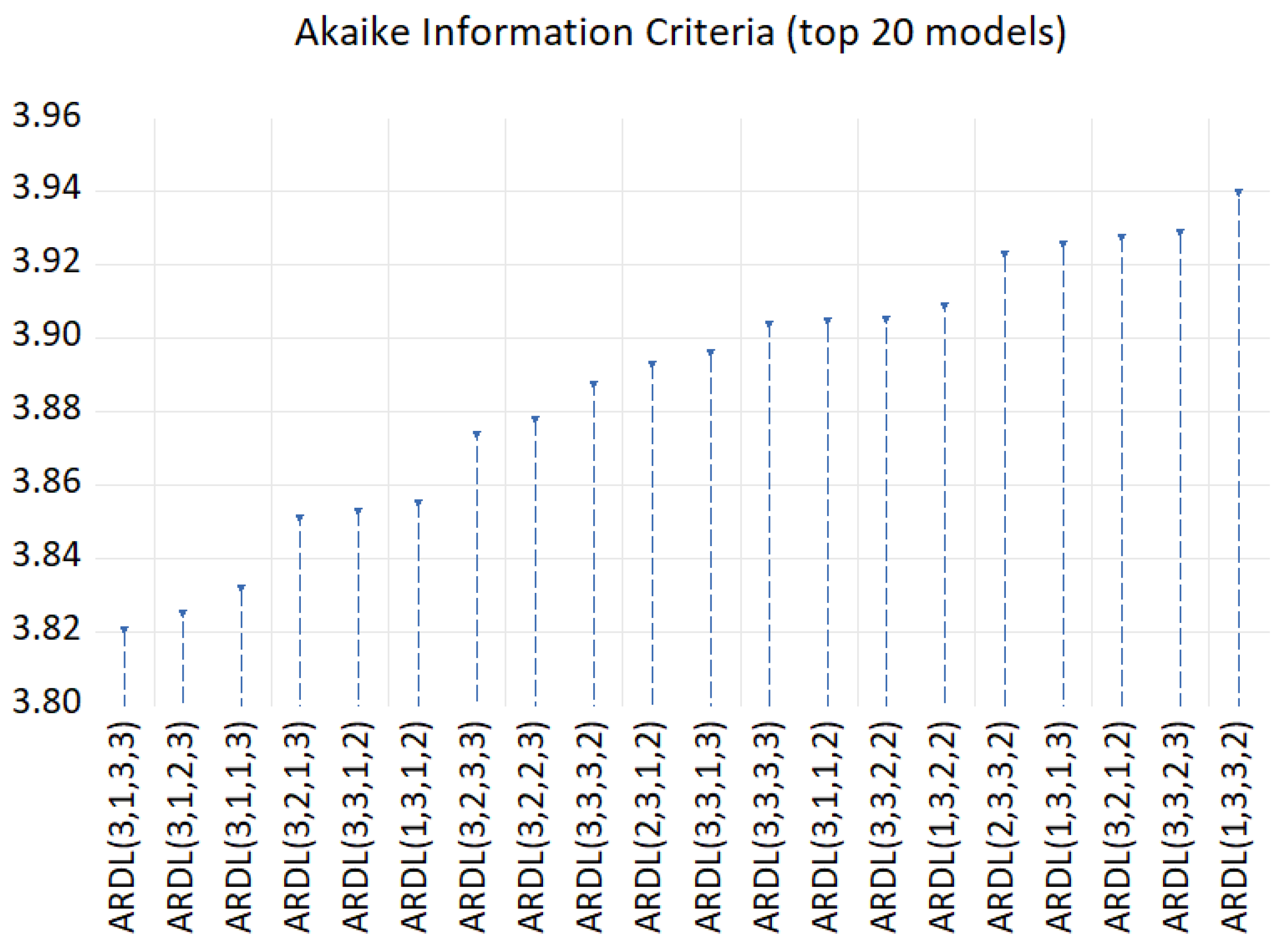
Figure A1 in Appendix A presents the Akaike information criterion values for the 20 best lag specifications. Because a lower AIC indicates a preferable balance between goodness of fit and model complexity, ARDL(3,1,3,3) is selected as the optimal specification because it records the lowest value among the competing models. The selected lag structure suggests that changes in financial development and the control variables may affect economic growth gradually rather than entirely within the current year. Nevertheless, the relatively small AIC differences among the leading specifications indicate that the model-selection advantage is modest; therefore, the results should ideally remain robust to closely competing lag structures.

4.7. NARDL Bounds Test

Table 7. NARDL bounds test for a long-run level relationship.

Sample Size	10% I(0)	10% I(1)	5% I(0)	5% I(1)	1% I(0)	1% I(1)
35	2.460	3.460	2.947	4.088	4.093	5.532
40	2.427	3.395	2.893	4.000	3.967	5.455
Asymptotic	2.200	3.090	2.560	3.490	3.290	4.370

Note: NARDL = nonlinear autoregressive distributed lag model. H₀ denotes the null hypothesis of no long-run level relationship. I(0) and I(1) denote the lower and upper critical bounds, respectively. k = 4 denotes the number of cointegrating regressors: FD⁺, FD⁻, TO, and GOV. FD⁺ and FD⁻ are the cumulative positive and negative components of the PCA-based financial development index; The specification includes a restricted intercept and no deterministic trend (Case 2). Effective estimation sample: N = 37.

presents the NARDL bounds test. The calculated F-statistic of 7.455 exceeds every reported upper critical bound, including the 1% finite-sample bound. The null hypothesis of no level relationship is therefore decisively rejected, confirming cointegration among economic growth, positive and negative financial-development components, trade openness, and government expenditure. Accordingly, short-run deviations occur around a stable long-run equilibrium relationship, although this finding alone does not establish causal direction.

4.8. Long-Run Coefficient Estimates

The estimated cointegrating relation reported by EViews is:

$${CE}_t={EG}_{t-1}-(0.401987{TO}_{t-1}+1.098588{GOV}_{t-1}-1.595537{FD}_{t-1}^{+}-0.874201{FD}_{t-1}^{-}-34.540410)$$

(8)

Panel A of

Table 8. Long-run coefficient estimates and standard-deviation-scaled conditional comparisons.

Panel A. Long-run coefficient estimates in the original regressor units
Variable	Coefficient	Std. error	t-statistic	p-value
Trade openness, TOt−1	0.401987	0.169008	2.378505	0.0235
Government expenditure, GOVt−1	1.098588	0.666112	1.649256	0.1089
Positive FD component, FD+t−1	−1.595537	0.833288	−1.914747	0.0645
Negative FD component, FD−t−1	−0.874201	0.594150	−1.471346	0.1510
Constant	−34.54041	19.02730	−1.815308	0.0789
Panel B. Standard-deviation-scaled long-run conditional comparisons.
Comparison		Signed change in the cumulative component (index units)	Estimated difference in annual GDP growth (percentage points)	Reported coefficient p-value
Increase in FD+ by SD(FD+)		+3.1380	−5.0068	0.0645
Decrease in FD− by SD(FD−)		−3.3707	+2.9467	0.1510
Increase in FD+ by the common benchmark SD(FD)		+1.5806	−2.5220	0.0645
Decrease in FD− by the common benchmark SD(FD)		−1.5806	+1.3818	0.1510

Note: Coefficients are derived from the conditional error-correction regression; restricted constant, Case 2 (restricted intercept and no deterministic trend). Note: SD denotes the sample standard deviation over 1980–2020, calculated using the N − 1 denominator. The first two rows use the standard deviation of each cumulative component separately. The last two rows use the same absolute change, SD(FD), to provide a common scale for expansion and contraction. Each estimated growth difference equals the corresponding coefficient in Panel A multiplied by the signed change shown in the second column. All comparisons hold the other cumulative component, trade openness, and government expenditure constant. Calculations use unrounded values. The p-values are those reported for the corresponding coefficients in Panel A; rescaling does not constitute a new significance test. These comparisons describe cumulative long-run differences, not one-period innovations or causal policy effects.

reports the long-run coefficient estimates in the original regressor units, while Panel B presents standard-deviation-scaled conditional comparisons. Trade openness has a positive and statistically significant coefficient of 0.402 (p = 0.0235), indicating that a one-percentage-point increase in trade openness is associated with an approximately 0.402-percentage-point increase in economic growth, holding other factors constant. Government expenditure has a positive but statistically insignificant coefficient.

To clarify the magnitude of the financial-development estimates, the coefficients are translated into standard-deviation-scaled comparisons using the statistics in Table 2, Panel B. The financial regressors are measured in index units, whereas the associated differences in the annual GDP growth rate are expressed in percentage points. A one-standard-deviation cumulative expansion is defined here as an increase in FD⁺ equal to its full-sample standard deviation of 3.1380 index units. This increase is associated with an estimated conditional long-run difference of approximately −5.007 percentage points in annual GDP growth, holding FD⁻, trade openness, and government expenditure constant. The corresponding coefficient has a reported p-value of 0.0645 and is therefore significant only at the 10% level.

A one-standard-deviation cumulative contraction corresponds to a −3.3707-unit change in FD⁻ and an estimated conditional long-run growth difference of approximately +2.947 percentage points, holding the other regressors constant. However, this estimate is statistically inconclusive at conventional significance levels (reported p = 0.1510) and should not be interpreted as evidence that financial contraction promotes growth. For comparison, Panel B also reports expansion and contraction benchmarks based on the same absolute change, equal to one standard deviation of the underlying FD index. These calculations are conditional long-run comparisons, not immediate responses to annual innovations or identified causal effects.

• Trade openness has a positive and statistically significant long-run association with economic growth: a one-unit increase in TO is associated with a 0.401987-unit increase in EG.
• The estimated long-run coefficient on government expenditure is not statistically significant.
• The constant is negative and statistically significant at approximately the 10% level.

4.9. Error-Correction and Short-Run Estimates

Table 9. NARDL error-correction and short-run coefficient estimates.

Variable	Coefficient	Std. Error	t-Statistic	p-Value
ECTt−1	−0.673547	0.089607	−7.516716	0.0000
ΔEGt−1	−0.314560	0.135669	−2.318585	0.0293
ΔEGt−2	−0.430215	0.110174	−3.904881	0.0007
ΔTOt	0.041379	0.067032	0.617306	0.5428
ΔGOVt	−0.394360	0.241201	−1.634983	0.1151
ΔGOVt−1	−0.284600	0.201805	−1.410271	0.1713
ΔGOVt−2	−0.349612	0.205820	−1.698627	0.1023
ΔFD+t	−0.703470	0.622543	−1.129994	0.2696
ΔFD−t	−1.710111	0.956850	−1.787231	0.0865
ΔFD+t−1	2.514159	0.786155	3.198045	0.0039
ΔFD−t−1	1.882552	1.408015	1.337025	0.1938
ΔFD+t−2	2.017842	0.687579	2.934706	0.0072
ΔFD−t−2	0.543278	0.999263	0.543679	0.5917

Note. Dependent variable: ΔEG. EViews labels the positive and negative FD terms @DCUMDP(FD) and @DCUMDN(FD), respectively—selected model: ARDL(3,1,3,3). The source output notes that p-values are incompatible with the t-bounds distribution.

presents the error-correction and short-run estimates. The error-correction coefficient is negative and highly significant (−0.674; p < 0.001), implying that approximately 67.4% of disequilibrium is eliminated within one year and confirming rapid convergence toward long-run equilibrium. The negative coefficients on lagged growth changes indicate short-run mean reversion. Trade openness and government expenditure have no statistically significant immediate effects. Positive financial-development shocks are insignificant contemporaneously but become positive and significant after one and two years, suggesting delayed growth benefits that are not sustained in the long run. The contemporaneous FD⁻ coefficient is significant only at 10%; because negative shocks enter FD⁻ with a negative sign, its economic effect has the opposite sign to the reported coefficient. Its lagged effects are insignificant and should not be overinterpreted. As summarized in

Table 10. Model specification and fit statistics.

Sample	1984–2020	Included Observations	37
Dependent lags	3 (automatic)	Models evaluated	192
Linear regressors	TO, GOV; max. 3 lags	Dual nonlinear regressor	FD; max. 3 lags
Deterministics	Restricted constant; no trend (Case 2)	Selection criterion	AIC
R2	0.828370	Adjusted R2	0.742555
S.E. of regression	1.247376	Mean dependent variable	−0.281081
Sum squared residuals	37.34270	S.D. dependent variable	2.458414
Log likelihood	−52.67129	Akaike information criterion	3.549799
F-statistic	9.652977	Schwarz criterion	4.115798
Prob(F-statistic)	0.000002	Hannan–Quinn criterion	3.749340
Durbin–Watson statistic	1.986820	Output date/time	20 August 2026, 22:52
Method	ARDL	Selected model	ARDL(3,1,3,3)

Note. The output reports automatic lag selection using AIC and a restricted constant without trend (Case 2).

, the model is jointly significant, explains approximately 82.8% of the variation in growth changes, and has a Durbin–Watson statistic close to two, although the small effective sample of 37 observations warrants cautious inference.

The error-correction coefficient is negative (−0.673547) and significant at the 1% level, supporting a long-run equilibrium relationship. Approximately 67% of any disequilibrium is corrected in the following year. Trade openness has no statistically significant short-run effect on economic growth. The contemporaneous effect of a positive financial development shock is negative but not significant. After one year, the effect becomes positive and significant, and it remains positive and significant after two years. Thus, increases in financial development do not raise growth immediately; the positive effect emerges with a lag. The contemporaneous effect of a negative financial development shock is negative and significant at approximately the 10% level; its lagged effects are not significant.

4.10. Long-Run and Short-Run Asymmetry Tests

Table 11. Coefficient symmetry tests.

Horizon	Variable	Statistic	Value	p-Value
Long run	FD	F-statistic	8.687207	0.0083
Long run	FD	Chi-square	8.687207	0.0032
Short run	FD	F-statistic	1.139054	0.2992
Short run	FD	Chi-square	1.139054	0.2859
Joint: long and short run	FD	F-statistic	7.436942	0.0041
Joint: long and short run	FD	Chi-square	14.87388	0.0006

Note. Null hypothesis: the relevant positive and negative coefficients are symmetric. Degrees of freedom: simple tests, F(1, 19) and χ²(1); joint tests, F(2, 19) and χ²(2).

presents the coefficient-symmetry tests. Both the F-test (p = 0.0083) and the chi-square test (p = 0.0032) reject the null hypothesis of long-run symmetry within the estimated specification. Short-run symmetry cannot be rejected, as both p-values exceed 0.28, whereas the joint hypothesis of long- and short-run symmetry is rejected at the 1% level. Although these tests provide evidence against the long-run equality restriction, the uncertainty surrounding the individual long-run coefficients and the small effective sample warrant caution. The results are therefore interpreted as suggestive evidence of long-run asymmetry requiring further confirmation, rather than as demonstrating a general feature of the Algerian economy.

The rejection of long-run symmetry provides specification-specific evidence that the estimated positive and negative long-run coefficients differ. However, the individual coefficients are not statistically significant at the 5% level (p = 0.0645 for FD⁺ and p = 0.1510 for FD⁻). Together with the small effective sample, this uncertainty calls for a qualified economic interpretation: the evidence of long-run asymmetry is suggestive and requires further confirmation. Short-run symmetry is not rejected. 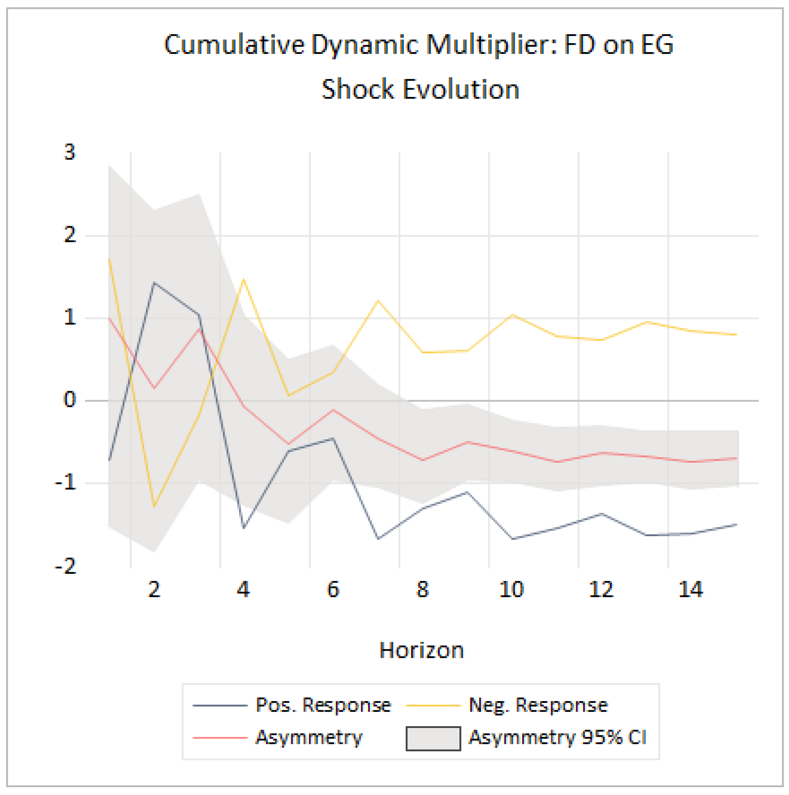Figure A5 in the Appendix B presents the corresponding model-based cumulative dynamic multipliers, which should be interpreted with the same caution.

4.11. Model Diagnostic and Stability Tests

Table A1. Diagnostic test results for the estimated NARDL model.

Test	Statistic	Value	Degrees of Freedom	p-Value
Breusch–Godfrey serial correlation LM	F-statistic	1.112949	F(2, 17)	0.3514
Breusch–Godfrey serial correlation LM	Obs. × R2	4.283712	χ2(2)	0.1174
ARCH heteroskedasticity	F-statistic	0.460038	F(1, 34)	0.5022
ARCH heteroskedasticity	Obs. × R2	0.480597	χ2(1)	0.4882
Jarque–Bera normality	Jarque–Bera	1.031188	—	0.597146
Ramsey RESET	t-statistic	0.102239	18	0.9197
Ramsey RESET	F-statistic	0.010453	F(1, 18)	0.9197
Ramsey RESET	Likelihood ratio	0.021480	χ2(1)	0.8835
Structural stability	CUSUM/CUSUMSQ	Within 5% bounds	—	—

Note. The Breusch–Godfrey test reported in this table examines serial correlation through two lags. Supplementary tests through three and four lags, together with the Breusch–Pagan–Godfrey heteroskedasticity test, are reported in Section 4.11. The ARCH test examines the absence of first-order ARCH effects, rather than homoskedasticity against all possible alternatives. The RESET auxiliary regression adds squared fitted values to the estimated ΔEG equation. 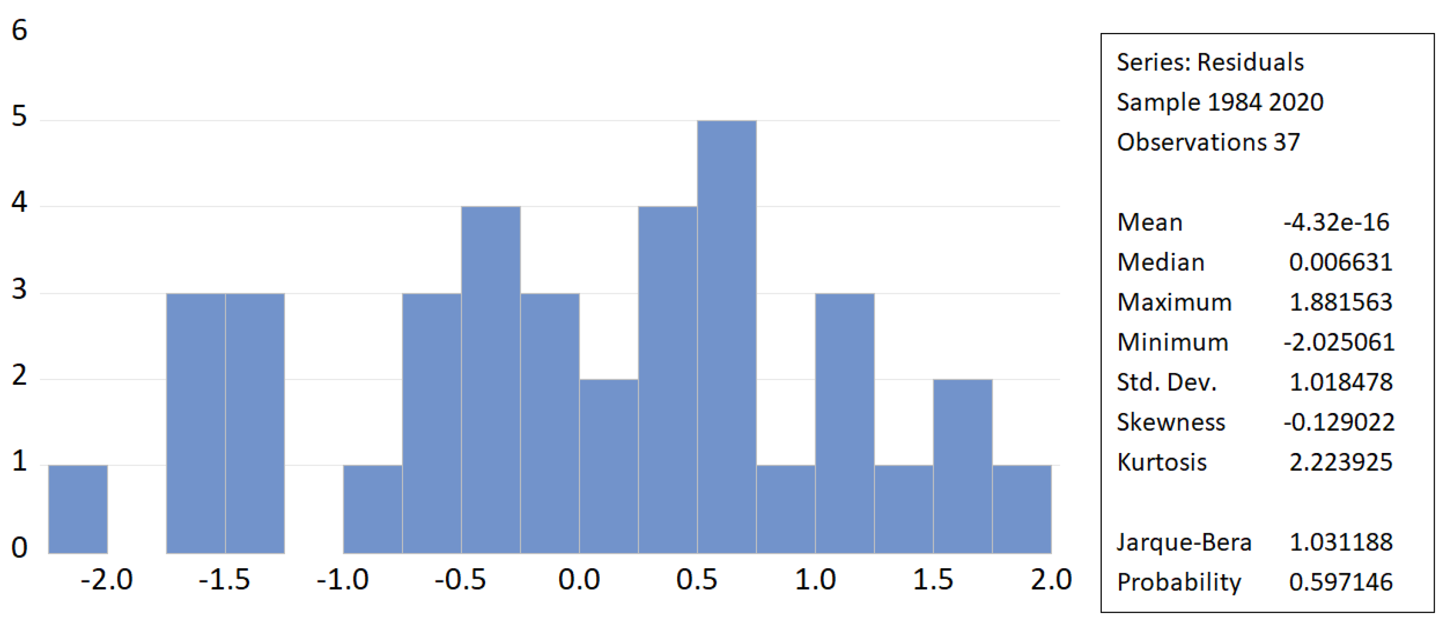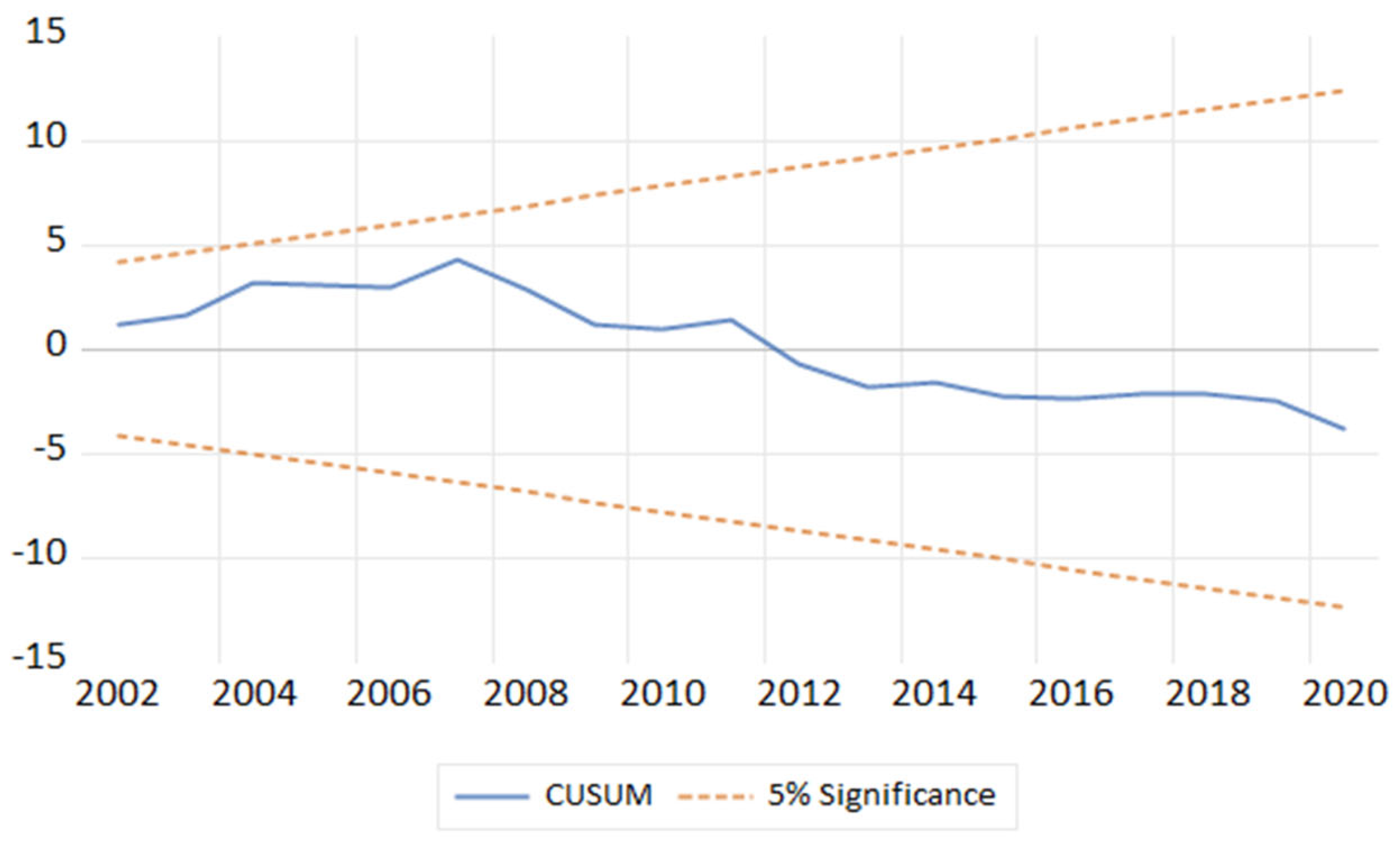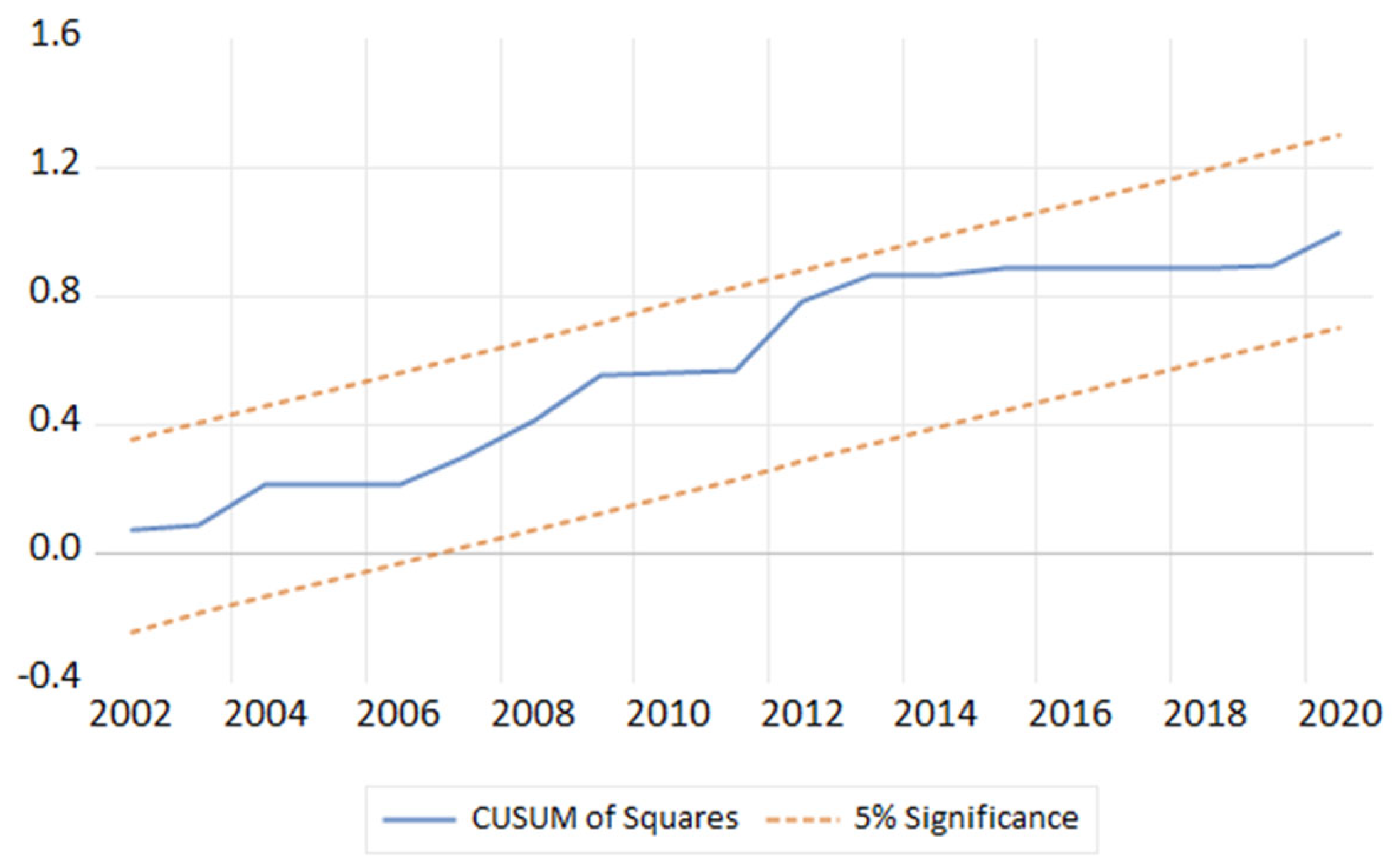Diagnostic non-rejection should be interpreted cautiously given the small effective sample.

and Figure A2, Figure A3 and Figure A4 report the original diagnostic and stability checks. Their interpretation must account for the effective sample of 37 observations and the 19 residual degrees of freedom in the full conditional error-correction equation. In this setting, diagnostic tests may have limited power, and non-rejection should not be interpreted as proof of adequate specification, homoskedasticity, or structural stability. The reported Jarque–Bera, ARCH(1), and Ramsey RESET tests do not reject their respective null hypotheses, but these outcomes remain conditional on the alternatives examined.

Supplementary tests were calculated from an independent reconstruction of the reported conditional error-correction specification, which reproduces the original BG(2) and ARCH(1) results to their displayed precision. The Breusch–Pagan–Godfrey test, using the original regressors in the auxiliary variance equation, yields a studentized Obs × R² statistic of 11.741921 with 17 degrees of freedom (p = 0.8155) and an auxiliary F(17, 19) statistic of 0.519569 (p = 0.9097). The test therefore does not reject homoskedasticity against the specified alternative. It complements, rather than replaces, the ARCH test. A full White specification with cross-products is not reported because its auxiliary design is saturated in this sample.

Higher-order serial-correlation checks provide less reassuring evidence. The Breusch–Godfrey test through three lags yields LM = 13.736433 (p = 0.0033) and F(3, 16) = 3.149172 (p = 0.0540). Through four lags, the corresponding statistics are LM = 15.503986 (p = 0.0038) and F(4, 15) = 2.704685 (p = 0.0705). The asymptotic LM statistics reject the null, whereas the auxiliary F-statistics indicate weaker evidence and reject only at the 10% level. The discrepancy is reported explicitly, and neither calibration is treated as having guaranteed exact finite-sample size. These results raise concerns about higher-order residual dependence and warrant further assessment of the dynamic specification.

The plotted CUSUM and CUSUMSQ paths remain within their displayed 5% boundaries. Nevertheless, the CUSUMSQ path in Figure A4 approaches the upper boundary around 2012–2013 before largely flattening over the subsequent years. This proximity merits caution but does not, without a boundary crossing, constitute a formal rejection or identify a structural-break date. Taken together, the diagnostics provide mixed and limited evidence about model adequacy; they do not establish unqualified structural stability or eliminate the possibility of misspecification.

5. Discussion

The findings confirm a stable long-run relationship among economic growth, financial development, trade openness, and government expenditure in Algeria. The negative and highly significant error-correction coefficient (−0.674) indicates that approximately 67.4% of deviations from long-run equilibrium are corrected within one year, suggesting relatively rapid adjustment. The Wald test rejects long-run symmetry within the estimated specification. Nevertheless, uncertainty around the individual long-run coefficients and the small effective sample warrant cautious interpretation. The results provide tentative support for H1 within the estimated specification, but further confirmation is needed before long-run asymmetry can be regarded as an established feature of the Algerian finance–growth relationship.

By contrast, we cannot reject short-run symmetry, indicating insufficient evidence that positive and negative financial-development shocks generate statistically different aggregate short-run effects. Accordingly, H2 is not supported. Nevertheless, positive financial-development shocks produce significant delayed positive effects after one and two years. This distinction is important because significant individual short-run coefficients do not necessarily imply overall short-run asymmetry when the corresponding Wald restriction cannot be rejected.

The results further indicate that financial expansion does not automatically translate into stronger economic growth over time. Positive financial-development shocks generate delayed short-run growth benefits, which may reflect the time required for changes in liquidity and financial intermediation to influence investment and productive activity. In the long run, however, the coefficient on positive financial-development shocks is negative and statistically significant only at the 10% level, providing relatively weak evidence that continued financial deepening may be associated with lower growth. This result should therefore be interpreted cautiously and does not imply that financial development is inherently detrimental to the Algerian economy. Rather, it suggests that finance’s contribution to growth may depend on intermediation efficiency and the productive use of financial resources. The long-run effect of negative financial-development shocks remains statistically insignificant and should consequently be regarded as inconclusive.

The standardized magnitudes also warrant caution. The estimated difference associated with a one-standard-deviation increase in FD⁺ is approximately −5.007 percentage points, which is about twice the sample standard deviation of annual GDP growth, 2.470 percentage points. This is a large conditional long-run comparison, not an estimated loss occurring within a single year. Moreover, the standard deviations of the cumulative components depend on the sample period and should not be interpreted as measures of typical annual financial shocks. Their observed ranges provide context for the scale of the estimates, but do not establish that a movement of this size, with all other regressors held constant, is directly observed in the sample. Consequently, these magnitudes require further confirmation and do not provide a basis for concluding that financial expansion necessarily reduces growth or that financial contraction improves it.

These findings are consistent with, but do not directly test, the hypothesis that the growth relevance of financial development may depend not only on financial depth but also on banking efficiency and credit quality. Demetriades and Rewilak (2020) and Xu (2025) provide evidence for these mechanisms in other settings, whereas the present model contains no direct measure of intermediation efficiency, credit composition, non-performing loans, or the productivity of financed activities. These mechanisms should therefore be regarded as plausible explanations requiring separate empirical verification. The weakly adverse long-run effect of positive financial-development shocks is also broadly consistent with Ho and Saadaoui (2022), who find that the growth contribution of bank credit diminishes beyond certain levels. At the same time, the results support Luintel et al. (2024), who argue that nonlinear finance–growth relationships are highly sensitive to the financial indicator, empirical specification, and country context rather than being characterized by a universal threshold.

The tentative support for H1 within the estimated specification contrasts with Al Khatib et al. (2023), who report symmetric finance–growth effects for Algeria using the IMF financial-development index. This difference suggests that how financial development is measured may materially influence empirical conclusions. The present study uses a PCA-based index constructed from liquid liabilities, private-sector credit, and bank deposits to GDP (%), thereby capturing several dimensions of financial depth simultaneously. The findings also differ from Appiah et al. (2026), who identify short-run but not long-run asymmetry in Ghana. Conversely, the broader conclusion that the finance–growth nexus is nonlinear and context-dependent is consistent with Chen et al. (2020) for Kenya and Elouaourti and Ibourk (2024) for Morocco. Taken together, these comparisons reinforce the importance of accounting for the direction of financial shocks, the time horizon, and country-specific financial structures when examining the finance–growth relationship.

Regarding the control variables, trade openness has a positive and statistically significant long-run association with economic growth, whereas its short-run effect is insignificant. This result is broadly consistent with Kong et al. (2021) and Bardi and Hfaiedh (2021), who show that the benefits of trade openness may emerge gradually through investment, technology transfer, competition, and improved resource allocation. The absence of an immediate short-run effect may therefore reflect the time required for these transmission mechanisms to influence domestic productive capacity. Government expenditure, by contrast, is statistically insignificant in both the short and long run. This finding is compatible with Ayad (2020), who documents short-run fiscal neutrality in several MENA economies, and with Ayana et al. (2023) and Khan et al. (2024), who emphasize that the growth effects of public spending depend strongly on expenditure composition, institutional quality, and government effectiveness rather than on aggregate expenditure alone.

Several limitations warrant caution in interpreting these findings. First, the effective estimation sample contains only 37 observations, which limits statistical power and makes inference particularly sensitive to model specification. Second, the principal long-run coefficient for positive financial-development shocks is significant only at the 10% level, while the long-run effect of financial contraction is statistically inconclusive. Third, the composite financial-development index captures financial depth but does not directly measure banking efficiency, sectoral credit allocation, non-performing loans, or the productivity of financed activities. The results therefore establish conditional empirical associations rather than direct causal mechanisms. In addition, structural changes over the 1980–2020 period may not be fully captured by the estimated specification.

Future research could address these limitations by extending the sample period, using quarterly or sectoral data, comparing alternative measures of financial development, and incorporating indicators of banking efficiency, institutional quality, non-performing loans, oil prices, and sectoral credit allocation. Additional robustness analyses using alternative lag structures, explicit structural-break models, threshold approaches, and identification strategies designed to address potential endogeneity would also help determine whether the observed long-run asymmetry remains robust across alternative specifications.

6. Conclusions

This study examined whether positive and negative changes in financial development have different short- and long-run effects on economic growth in Algeria from 1980 to 2020. Using a composite financial development index constructed through principal component analysis and a nonlinear autoregressive distributed lag (NARDL) model, the analysis provides evidence of a stable long-run relationship among economic growth, financial development, trade openness, and government expenditure. The Wald test rejects long-run symmetry, although neither individual long-run financial-development coefficient is statistically significant at the 5% level. The results tentatively support H1 within the estimated specification, but further confirmation is needed before long-run asymmetry can be regarded as an established feature of the Algerian finance–growth relationship. Short-run symmetry is not rejected, indicating insufficient evidence that positive and negative financial-development shocks have significantly different aggregate short-run effects. Accordingly, H2 is not supported.

The empirical results further show that positive financial-development shocks generate delayed positive effects on economic growth after one and two years in the short run. In the long run, however, the coefficient associated with positive financial-development shocks is negative and statistically significant only at the 10% level. In contrast, negative shocks are statistically insignificant. These findings should therefore be interpreted cautiously and do not imply that financial development is inherently detrimental to economic growth. Rather, the estimated patterns suggest that the relationship may vary with the direction of financial changes and the time horizon, although the long-run asymmetry evidence requires further confirmation. Trade openness is positively and significantly associated with economic growth in the long run, whereas government expenditure does not exhibit a statistically significant effect. In addition, the negative and highly significant error-correction coefficient indicates relatively rapid convergence toward long-run equilibrium, with approximately 67.4% of disequilibrium corrected within one year.

The study contributes by combining a PCA-based financial-development index with an NARDL framework to investigate potential asymmetries in Algeria. Its empirical findings provide suggestive, rather than conclusive, evidence of long-run asymmetry. By distinguishing between positive and negative financial-development shocks, the analysis demonstrates that a conventional symmetric specification may conceal important differences in the long-run response of economic growth. The findings also add to the limited country-specific evidence on nonlinear finance–growth relationships in hydrocarbon-dependent and bank-based economies.

From a policy perspective, the findings are consistent with the hypothesis that the quality and allocation of financial resources may matter for growth. However, the present model does not identify these mechanisms directly. Banking efficiency, credit composition, non-performing loans, and sectoral allocation should therefore be treated as hypotheses for further investigation rather than as policy implications derived from the estimated coefficients.

Several limitations should be acknowledged. The relatively small annual sample, the marginal statistical significance of the principal long-run financial-development coefficient, the inconclusive effect of financial contraction, the use of aggregate financial indicators, and potential endogeneity constrain the results’ generalizability. Moreover, the model does not directly capture banking efficiency, credit allocation, institutional quality, or sectoral differences. Future research could extend the sample period, employ higher-frequency or sectoral data, compare alternative measures of financial development, and incorporate variables such as oil prices, institutional quality, non-performing loans, and sectoral credit allocation. Alternative nonlinear specifications, explicit structural-break models, and identification strategies designed to address potential endogeneity would also provide useful robustness checks and help clarify the causal mechanisms underlying the finance–growth relationship in Algeria.