Abstract
The effects of initial institutions and change in institutions on the growth of ex-socialist countries is unsettled in the literature. This is due to difficulties in modeling the effects of institutions and their change. The objective of this paper is to contribute to this area. Ex-socialist countries faced heterogenous initial conditions at transition. Those that joined the EU experienced institutional integration as well as institutional improvement. Using publicly available data from about ten years before and after EU accession and two-way fixed effects differences-in-differences estimation, this paper finds that these countries experienced growth boosts post-EU accession. Achieving institutional integration cum improvement by accepting and implementing EU’s regulations and norms in all details permitted this boost. The initial conditions mattered—the effect was greater in “new” ex-socialist countries (which had the additional burden of creating new administrative structures and economic relationships) than in the “old.” Using the neo-classical growth model, the paper then examines whether this boost in growth was due to a higher contribution of inputs or due to an increase in the efficiency with which inputs were used. It indicates that it was due to increased contribution of human capital rather than an increase in the amount of human capital or other economic or political confounders. These countries’ skilled labor, already high in skills at transition by OECD standards, needed the right institutions to unlock its potential.
1. Introduction
The role of institutions in growth has been recognized from the very beginning of economics. Smith (1776) highlighted the role of the protection of private property in specialization and exchange and innovation and growth. Mauro (1995), and Knack and Keefer (1997), and Hall and Jones (1999) were among the first to empirically establish a relationship between institutions and growth. Rosenberg and Birdzell (1996) explain the critical link between institutions favoring commerce and the emergence of corporations and the higher income of Europe and the West. Morck et al. (2005) emphasize that good institutions in the private sector are important for growth. Comparing the roles of institutions, geography, and international trade in growth, Rodrik et al. (2004) find the role of institutions to be dominant. In their survey, Acemoglu et al. (2005) place institutions as the central factor for growth. Inter-country economic inequality is often ascribed to differences in institutions. Alfaro et al. (2008) show that capital does not flow from rich countries to poor countries due to the latter’s poor institutional development. This lack of capital movement from rich countries with low marginal returns to poor countries with presumably high marginal returns was first pointed out by Lucas (1990) and came to be known as the Lucas Paradox. Papaioannou (2009) reaches similar conclusions as Alfaro et al. (2008). C. J. Jones and Romer (2012) highlight four state variables, namely ideas, population, human capital, and institutions, as central to growth/development theory. They model the first three but refrain from modeling institutions.
The objective of this study is twofold: The first is to examine the role of initial (say, at-transition) institutions and a change in institutions (say, upon joining the EU) in affecting growth. Theory expects a positive effect. The paper confirms it for ex-socialist countries that joined the EU (using two-way fixed effects DID estimation). The second objective is to examine whether the positive effect was due to inputs or due to the efficiency with which they were used. Theory makes no prediction. The paper estimates a neo-classical growth model by panel estimation separately for the period before the said countries joined the EU and after accession to discover whether the statistical significance of the proximate factors differed after accession. The motivation for the study is to contribute to the literature linking institutions to growth.
Ten (EU10) ex-socialist countries joined the EU in the mid-2000s—eight on 1 May 2004 and two on 1 January 2007. To analyze the effects of initial conditions, this paper divides them into three groups. The first group consists of Czechoslovakia, Hungary, and Poland, which have been sovereign countries since the Second World War and formed the Visegrád alliance in 1991. Its membership increased to four after the friendly break-up of Czechoslovakia in 1993 into the Czech Republic and Slovakia. These are referred to as “old” ex-socialist countries or the Visegrád Four (V4). They joined the EU on 1 May 2004. The other four countries that joined the EU on 1 May 2004—Estonia, Latvia, Lithuania, and Slovenia—(ELLS) are called “new” ex-socialist countries, having emerged as separate countries in 1990/1991 from the break-up of the Soviet Union or Yugoslavia. Bulgaria and Romania (B&R), which joined the EU on 1 January 2007, are considered a separate group due to their later accession to the EU and the lower level of institutions in 1996 (1996 is the first year that data on institutions is available, precluding their use in econometric estimation that starts from 1991. See, World Bank, 2024).
The literature review in Section 2 reveals various sociological determinants of institutions: the extent of socialist elites’ entrenchment (Beck & Laeven, 2006), rent seeking by the elite and powerful interest groups (Melki, 2022), the organization of exchange in transparent versus opaque business networks (Van Ees & Bachmann, 2006), and trust within enterprise networks (Johnson et al., 2000). The institutional integration of the ex-socialist countries with the EU was unlike earlier rounds of EU expansion (see Campos et al., 2019)—these countries had not been capitalist democracies for at least four decades (mostly since the Second World War). The pre-2004 EU (EU15) required the EU10 to undertake various institutional improvements before the latter could join it. This paper examines whether joining the EU and adopting its norms and standards boosted the growth of the ex-socialist countries. Building on Bohle’s (2018) finding of institutional development upon joining the EU, this paper examines whether Van Ees and Bachmann’s (2006) expectation that the change in institutions upon joining the EU would lead to a boost in growth was realized. It examines this question in the context of differing initial adverse institutions in the ex-socialist countries that joined the EU. Specifically, it examines whether countries with initial low institution levels or those burdened with creating institutions due to emerging as independent countries in 1990/1991 from larger political units had a greater gain. Furthermore, it investigates whether greater growth was driven by one or more inputs or the efficiency with which inputs were used (TFP).
Penn World Tables (PWT) data, available at http://www.rug.nl/ggdc/productivity/pwt accessed on 2 January 2021, is used in the paper. The paper uses two-way fixed effects difference-in-difference (“TWFE DID”) estimation (see, e.g., Ashenfelter & Card, 1985) to examine the effects of joining the EU on income and panel estimation of a neo-classical growth model to discover the proximate factor(s) behind any growth effect found. This paper addresses important questions: whether an improvement in institutions of ex-socialist countries boosted growth, how the boost may have depended on initial institutions, and the relative importance of input amounts and TFP in affecting growth. The first question has been examined for the 2004 Eastern enlargement of the EU by describing EU accession as institutional integration (but not recognizing the institutional improvement) and using the synthetic control method (Campos et al., 2019). It achieves different results. The other two questions (as far as the author knows) have not been examined.
In Section 2 below, the paper undertakes a review of the relevant literature. Section 3 describes the DID model for estimating whether EU accession boosted growth and the neo-classical growth model specification used to discover the proximate causes of the effects shown by the DID model. Section 4 explains the data used, presents non-econometric analysis of DID growth rates, and examines dynamics. Section 5 estimates the effects of EU accession on income by a TWFE DID model and describes institutional changes around EU accession qualitatively. Section 6 examines proximate factors for B&R and “old” and “new” ex-socialist countries for both the pre-accession and post-accession periods. Section 7 contains concluding observations, including the implications of our analysis.
2. Literature Review
This review is of how institutions have been defined and to what extent their role in growth has been studied in the context of ex-socialist countries of Europe. For completeness, it also includes human capital theories.
The seminal work on institutions is by North (1981), who defines institutions as “a set of rules, compliance procedures, and moral and ethical behavioral norms designed to constrain the behavior of individuals in the interests of maximizing the wealth or utility of principals” (pp. 201–202). Nunn (2014) describes that rules may either be codified in written laws, regulations, and instructions or they may be cultural traits, unwritten conventions, and practices. Fuchs-Schündeln and Hassan (2015, p. 43) define institutions more precisely. They define institutions as “the broad set of rules, regulations, laws, and policies that affect economic incentives and thus the incentives to invest in technology, physical capital, and human capital”.
Human capital goes beyond credentials to training and education that are useful for production. Its theories either emphasize individual choice of education with minimal state role or recognize the role of the state in it. Under the former, individuals have an incentive to invest in education without goading by the state. The seminal work for it is by Becker (1962), who focused on the choice of a representative individual for education and training in line with microeconomic theory. However, even with its microeconomic foundations, the motivation for studying human capital was macroeconomic—the role of learning in economic development, in explaining the Solow (1956) residue, and as an additional factor of production. On the other hand, one of the cofounders of human capital theory, Schultz (1960), emphasized and recognized the role of public education in developing human capital.
Glaeser et al. (2004) and Beck and Laeven (2006) analyze the role of initial institutional conditions on growth levels and reach opposite conclusions. The former, analyzing political institutions, find constraints on the executive to be less significant than human capital as a fundamental source of growth. Beck and Laeven (2006) show that institutional quality varied greatly among 24 ex-socialist countries and was adversely affected by the extent of socialist elites’ entrenchment (positively related to years under socialism) during the immediate transition period, which, in turn, positively influenced their first decade of growth.
Melki (2022) investigates the consequences of income inequality on investment in diverse institutional contexts, demonstrating that the adverse effect disappears when property rights improve, rent seeking by the elite decreases, and the rule of law is secured. Van Ees and Bachmann (2006) emphasize the importance of organizing exchange in transparent versus opaque business networks for growth. The transition economies no longer had the centrally planned economic structure of networks in which economic transactions take place. Instead, new obscure networks emerged to exploit and benefit from a high degree of complexity and uncertainty, which does not facilitate value-creating activities. Kowalewski and Rybinski (2011) similarly argue that powerful interest groups can alter their legal and economic environment to be more self-serving when financial, legal, and political institutions are weak; Beck and Laeven (2006) suggest that the socialist elite remained an entrenched interest group in the initial phase of transition. Johnson et al. (2000) highlight the importance of trust within a network of enterprises for building new economic structures after the transition. By a meta-regression analysis of 46 studies of the effects of reforms over four to eight years on growth rates in transition economies, Babecký and Campos (2011) find that studies that include initial macroeconomic and structural distortions had a decrease of 0.6 in statistically significant t-value (with the average being 1.7).
The task of transition is to build trust-based institutions and exchange networks in a situation of weak legislators and ineffective regulation by both markets and by regulatory agencies. Van Ees and Bachmann (2006) suggest that the 2004/2007 enlargement of the EU was likely to foster transparent Eastern–Western firm networks and favorable macro- and meso-institutional frameworks. Bohle (2018), comparing Visegrad and Baltic countries, discusses how the EU exported its rules, regulations, and norms to Central and East European countries as they sought membership.
Campos et al. (2019), following the distinction by Lawrence (1996) between shallow integration (trade agreement and other border measures) and deep integration (which includes competition and regulatory policies, as well), define the former as economic integration and the latter as institutional integration. Identifying EU enlargement as institutional integration, they study the growth effects of EU enlargement from 1973 to 2004. The pre-2004 EU enlargement was to the U.K., Ireland, and Denmark (in 1973); Greece (in 1981), Spain, and Portugal (in 1986); and Austria, Finland, and Sweden (in 1995). However, the 2004 Eastern enlargement was like no other before it. The EU sought to reinforce “the applicant states’ capacity to maintain the rule of law, uphold economic freedom, prevent discriminatory practices, foster domestic competitiveness and implement European rules and policies,” (Bohle, 2018). Section 5.2 refers to many institutional changes these countries adopted to obtain EU accession. The EU10’s lack of comparable capitalist and democratic experience led the EU15 to ensure the EU10’s institutional development, as well.
Campos et al. (2019, p. 54) obtain mixed results for the 2004 Eastern enlargement, “with benefits that are positive and large for some countries, while weak or even negative for others”. They ascribe the weak results to the long preparation process and the anticipation effects. If their accession year is considered as 1998 (since the European Council established the process of Eastern enlargement in December 1997), the mixed results disappear. They create synthetic controls for each of these countries (with the accession year considered as 1998) based on a donor pool mostly from Asian and Latin American countries. Their synthetic Czech Republic is based on South Korea, Japan, Thailand, and Albania; synthetic Estonia on Croatia, Turkey, and Columbia; synthetic Hungary on Mexico, Canada, Ukraine, Colombia, the Philippines, and 19 other unspecified countries; synthetic Latvia on Columbia, Croatia, Morocco, Mexico, and Turkey; synthetic Lithuania on Turkey, Russia, and Ukraine; synthetic Poland on Croatia, Malaysia, Colombia, South Korea, Uruguay, and 20 other unspecified countries; synthetic Slovakia on Croatia and South Korea; and synthetic Slovenia on South Korea, Chile, Canada, Columbia, and Thailand.
Campos et al. (2022) elaborate that institutional integration includes delegating to a supra-national entity control over select policies. Identifying economic integration with EEA membership, they emphasize the distinction between economic integration and institutional integration by considering Norway. Norway joined the EEA in 1995 but not the EU. (Norway is the only such major country. The other EEA countries that are not members of the EU are Iceland and Liechtenstein.) Using each of the sectors in the 19 NUTS 3 regions in Norway as the treatment unit and the corresponding sectors from all (75) NUTS 3 regions of Austria, Finland, and Sweden as the counter-factual in addition to the synthetic DID method, they find that Norway’s regional productivity, on average, was 0.6% lower annually for seven years because of Norway not joining the EU.
Describing the EU as the most integrated economic integration in in the world today, Cieślik and Turgut (2021) examine the effects of 2004 EU accession by eight East and Central European ex-socialist countries on their population-weighted average income by using the synthetic control method. They use Armenia, Croatia, Israel, and Ukraine to create their single synthetic control unit for the EU8 and find the immediate impact of their EU accession was modest but had a greater impact once they joined the Schengen zone in 2007 and could more completely benefit from the Common Market. Felbermayr et al. (2016) estimate that abolishing border controls on trade under the Schengen agreement was equivalent to a reduction in tariff by 0.7 percentage points. The growth rate of the said GDP per capita for 2004–2012 was 2.7% larger than that of the synthetic EU8.
Rather than develop the synthetic control method, Callaway and Sant’Anna (2021) develop the staggered DID procedure for estimating the average treatment effect of treatment (ATET) when (a) there are multiple pre-treatment and post-treatment periods, (b) different units are treated in different years, and (c) the parallel pre-treatment assumption holds only when conditioned on observed variances. They propose group–time average treatment effects, ATET (g, t), to capture the ATET in period t of the group of units first treated in period g to be estimated by a well-defined treatment effect parameter in the regression. Baker et al. (2022) report that staggered DID is used heavily in Finance and Accounting and is susceptible to both Type-I and Type-II errors. They suggest alternative estimators.
Kantorowicz and Spruk (2024) focus on institutional reform in 24 ex-socialist countries. By institutional reform they mean an all-encompassing transformation of a planned economy into a market economy. While recognizing that East and Central European countries that joined the EU transformed successfully, they do not examine whether EU accession played a role. They compare big bang (see Dehejia, 1996; Hoen, 1996) versus gradualist approaches to transformation into a market economy by these 24 countries. They find a sustained big bang approach is the most effective, while an abortive, gradualist approach produces a complete breakdown of growth trajectories.
This paper examines the effects of institutional integration cum improvement and of initial institutions on the growth of 10 ex-socialist countries that joined the EU in the mid-2000s. The closest papers to our study are by Campos et al. (2019) and Cieślik and Turgut (2021). Unlike this paper, Campos et al. (2019) and Cieślik and Turgut (2021) do not highlight the role of institutions, do not examine whether the effects of accession on income by “new” ex-socialist countries differed from the “old,” do not examine the effects for the 2007 accession countries, and do not study which proximate factor was behind the boost in income upon accession. Below, we compare this study to the work of Campos et al. (2019) and Cieślik and Turgut (2021) for the question all three papers study, namely, the effect of 2004 accession on income and growth.
3. Methodology, TWFE DID and SCM, and Neo-Classical Growth Model
The basic hypothesis of this paper is that an improvement in institutions of ex-socialist countries, whether from the initial low level or upon EU accession, boosted their growth. Section 3.1 describes the methodology of the two-way fixed effects (TWFE) DID model used to estimate the effects of joining the EU; Section 3.2 compares the TWFE DID method with the synthetic control method, while Section 3.3 outlines the neo-classical growth model employed to determine the proximate determinants of the accession countries’ growth both pre-accession and post-accession. The data for both the TWFE DID model (Section 3.1) and the neo-classical model for all the countries is available and collected for the 1991–2014 period.
3.1. Two-Way Fixed Effects Difference-in-Differences Model
Econometric methods to study institutions can be grouped into the following: instrumental variables, regression discontinuity, and difference-in-differences (DID). These methods are central to the “credibility revolution” in empirical economics. For more details, see Angrist and Pischke (2010). Among the three methods, DID is likely the most frequently applied. For example, Callaway and Sant’Anna (2021) call it “one of the most popular research designs”, and, as more fully explained below, Currie et al. (2020) find that in their dataset, 25% of all micro papers refer to DID. Examples of the use of DID to study macroeconomic relationships are the work of Rodrik and Wacziarg (2005), Papaioannou and Siourounis (2008), and Ehrlich et al. (2018).
Let Yist represent the outcome in country i in group s at year t; Treat indicate country i’s treatment status in the year of treatment, that is, Treat = 1 if country i is a treatment country and = 0 if it is a not; and Postt indicate the post-treatment period, that is, Postt = 1 ∀ t ≥ treatment year and = 0 otherwise. Then, the specification of a two-way fixed effects DID model is
where β gives the average treatment effect of treatment, ATET, αi and γt indicate country and time fixed effects, respectively, and εist is the error term. This specification allows for any correlation between the treatment dummy and country features since the outcome effects of the latter are captured by αi (Persson & Tabellini, 2008).
Yist = αi + β Treat × Postt + γt + εist
DID design uses the time trend of the untreated group as the counter-factual. The counter-factual is no change in the EU membership and the treatment is joining the EU. The paper does not use a staggered DID approach because the treatment is binary, it takes place at the same time for all countries in each of the three treatment groups, V4, ELLS, and B&R, and the pre-treatment parallel trend assumption is satisfied for all three groups.
Countries whose membership status in the EU did not change can be used as the control group. There are two such groups of countries: the first is the “old” EU (EU15), and the second group consists of “new” ex-socialist countries that did not join the EU and became the core of CIS. Countries from the EU15 are used as the control group since their economic structure is closer to that of the EU10. The energy sector is dominant in CIS countries in the sample (Kazakhstan and Russia) or agriculture (Armenia, Kyrgyzstan, and Tajikistan), and a majority (Armenia, Kazakhstan, Kyrgyzstan, and Tajikistan) are located in Asia. Following Campos and Coricelli (2002), who suggest that countries at similar levels of per capita income and economic structure should be used as comparators, the counter-factual from the EU15 would be most applicable. Accordingly, this paper uses four EU15 countries—whose average income for the estimation period (1991–2014) was closest to that of the EU10. These countries are France, Greece, Portugal, and Spain, “FGPS.” In fact, using FGPS as the control group (instead of CIS) is more conservative for the effects of EU accession on income, since the EU10’s income relative to that of FGPS increased less (by 20 percent—from 0.65 to 0.80) during the estimation period than the EU10’s income relative to that of CIS (which almost doubled—from 1.4 to 2.7).
FGPS already had a relatively high level of institutional development. EU10 countries received the same treatment: a set of measures and regulations that EU membership required. Their membership in the EU occurred only after adopting/agreeing to adopt EU rules, regulations, and norms as well as agreeing to being subject to the EU’s (newly created) monitoring and surveillance mechanisms. As noted above, the EU sought to reinforce “the applicant states’ capacity to maintain the rule of law, uphold economic freedom, prevent discriminatory practices, foster domestic competitiveness and implement European rules and policies,” (Bohle, 2018, p. 8). The EU did that to ensure that the EU10 not only institutionally integrated with the EU but also reached the same level of institutional development as the EU15, including FGPS. The method used in the paper (TWFE DID) is suitable to evaluate the effects of institutional integration and institutional development that the EU10 achieved after agreeing to such externally imposed conditions.
3.2. TWFE DID and Synthetic Control (SC) Methods
This sub-section compares the two-way fixed effects DID (TWFE DID) and synthetic control (SC) methods and give reasons for choosing the former.
Currie et al. (2020) find that although in their dataset (NBER papers from 1 January 1980 to 30 June 2018 and papers in “top five” economics journals between 1 January 2004 and August 2019), the first paper using DID was published only in 1985 (Ashenfelter & Card, 1985), about 30 years later, 25% of all micro papers refer to DID. They also note that SC, although a newcomer (it was introduced by Abadie and coauthors (Abadie & Gardeazabal, 2003; Abadie et al., 2010, 2015)), has made rapid advance since 2010.
The fundamental assumptions of TWFE DID and SC methods are closely related (Arkhangelsky et al., 2021). TWFE DID assumes the pre-treatment trend lines of treated and control units are parallel—permitting additive fixed unit effects. It is bedeviled by the problem of finding a robust counter-factual that satisfies the parallel trend-line assumption. See Boltho and Eichengreen’s work (Boltho & Eichengreen, 2008). SC creates a synthetic control unit by weighting non-treated units so that its pre-treatment trend is matched or aligned (not just parallel) to the treated unit. It is bedeviled by the problem of creating this synthetic control unit that matches. Campos et al. (2022) observe that by using a convex combination of control units, matching allows for a better counter-factual than DID (which is based on a simple average). However, both DID and SC methods assume the control or donor units are not affected by the treatment. Since the direction of the spillover effects is hard to determine, most researchers ignore the spillover effects of treatment. The pre-treatment matching permits time-varying un-observables, while DID can only permit time-invariant and common trend effects. Abadie et al. (2015) explain that since the weights can be restricted to be positive and sum to one, SC prevents extrapolation that a DID regression does not, since the regression weights can be outside the [0, 1] interval. Since matching requires that each treated unit has a separate matching synthetic unit, Arkhangelsky et al. (2021) observe that DID is used when there are a substantial number of units treated and SC when there is a single (or a small number of) unit treated.
Grier and Grier (2021) point out the following. A TWFE DID ATET gives a weighted average of the individual treatment effects. If the treatment effects are heterogenous (for example, if the later adopters have a different average effect than the earlier adopters), ATET is biased and may even have the opposite sign of the true effect. On the other hand, unit effects given by the synthetic (or matching) control method are simply averaged (unweighted) so that the ATET is unbiased under staggered treatment and treatment effect heterogeneity. The chief concern with the synthetic control method is that there may be time-invariant un-observables that affect selection into both control and treatment variables that cannot be controlled in the matching process. The TWFE DID simply sweeps away the un-observables. An and Winship (2017) suggest using the synthetic control method after differencing so that the un-observables are removed.
The treatment effect in the matching method is not a coefficient in a regression as in TWFE DID. Once the exact matching is accomplished, the treatment effect is simply the difference between the outcome in the treated unit and that in the synthetic control unit. It thereby permits an examination of the dynamics of the post-treatment effect, which TWFE DID cannot do. However, sometimes exact matching may not be feasible. That will be the case when the characteristics to match are many. There is also a question of choice of implementing the matching method. Grier and Grier (2021) use four types of methods: matching to the nearest neighbor, to the average of two nearest neighbors, and to the average of three nearest neighbors, and kernel matching. Campos et al. (2022) first match by sector all 19 NUTS 3 regions of Norway to all 75 NUTS 3 regions of Austria, Finland, and Sweden (multiple-treated), and then they match each sector of a NUTS 3 region of Norway to the same sector of regions of Austria, Finland, and Sweden (single-treated).
This paper chooses the TWFE DID empirical model over the SC method for the following reasons. The author was able to find a robust counter-factual that met the parallel pre-treatment trend lines of treated and control units required for TWFE DID. The control units were also in Europe and as close in per capita income (indicating a similar economic structure) as the treated units. Since the SC method matching is exact, the time-varying pre-treatment un-observables permitted by it are a problem—they may also vary post-treatment. Then, the effect shown by it will not only show that of the treatment but also that of the varying un-observables post-treatment. Since the paper considers that all units in the three groups, V4, ELLS, and B&R, adopt the treatment simultaneously, the advantage the SC method has with staggered adoption is not relevant. Also, this paper is not interested in the dynamics of the treatment effect but in the overall effect of treatment for which TWFE DID is quite suitable.
The variables needed by the TWFE DID are the sample values of the objective of treatment for both the treated and control units. This paper’s objectives are to study the effects of joining the EU on income. It needs data on the per capita income of treated and control countries for the sample period.
3.3. Neo-Classical Growth Model and Proximate Factors for Growth
The paper uses kl for physical capital per unit of employed labor, h for average human capital (that is, quality of labor or average educational attainment) in a country, and A for the efficiency with which physical capital and human capital are used, namely, TFP. (The main problem in developing the human capital measure is constructing data on average years of schooling. Inklaar and Timmer (2013) explain that PWT 9.0 uses average years of schooling data for 95 countries primarily from Barro and Lee (2013) and for 55 countries primarily from Cohen and Leker (2014) and Cohen and Soto (2007), and the assumed rate of returns to years of schooling on Mincerian equations links the two around the world as in Psacharopoulos (1994).) These factors, physical capital, human capital, and TFP, are called “proximate” causes by Rodrik (2003) and distinguished from “fundamentals” for growth like trust, geography, institutions, culture, and genetic distance. Using the neo-classical growth model, the left-hand side then would be the output per unit of employed labor. Let per capita income, yJ, approximate output per worker and ignore the time sub-scripts. Then, for Country J,
yJ = AJ klJα hJ1−α
The paper uses income relative to the US as the dependent variable—since, as noted by B. F. Jones and Olken (2008), US income has been the least volatile since the Second World War. It helps in estimation by making data both more granular and less vulnerable to the effects of world/region-wide factors on income. Like Kutan and Yigit (2007), the paper also cannot use Germany as the benchmark or numeraire county because data is for unified Germany (including the ex-socialist East Germany).
(2) tells us that Country J’s income depends on its TFP, its capital–labor ratios, and its average human capital. Our purpose is to investigate how much of the change in Country J’s income is due to a change in its TFP versus changes in its capital–labor ratios or in its level of average human capital. Taking total derivative ΔyJ/Δt, letting Δt = 1, adding constant, µ, and error, ε, terms, and representing coefficients of the derivatives of the RHS ratio variables by β1, β2, and β3, respectively, gives
ΔyJ = µ + β1 ΔAJ+ β2 ΔklJ + β3 ΔhJ + ε.
The R2 of an equation like (2) (which is estimated for a panel of countries) cannot be, and is not expected to be, 1. See the value of R2 for proximate factors’ panel regressions. TFP is not the residual after the effects of physical capital–labor ratio and human capital–ratio are removed from the said panel’s output. The slope coefficients of (3) are assumed positive and are interpreted as follows: an increase in Country J’s explanatory variable leads Country J’s income to increase. If the paper finds that EU accession positively affected income, it would be interested in examining whether the positive effect can be ascribed to a specific proximate factor.
4. Data, Descriptive Analysis, and Dynamics
4.1. Data
The paper uses PWT 9.0 country data for 1991–2014. The country data are not combined into regional data for any group of countries. PWT 9.0 derives the data on human capital from the years of schooling (from Barro and Lee, 2013) and the rate of returns to education from a Mincerian equation linking the two around the world. As explained above, France, Greece, Portugal, and Spain, “FGPS”, are used as control countries. That is, the paper compares the growth of ex-socialist countries, divided into three groups, V4 (the Czech Republic, Slovakia, Hungary, and Poland), ELLS (Estonia, Latvia, Lithuania, and Slovenia), and B&R (Bulgaria, and Romania), to similar growth of FGPS.
4.2. Descriptive Analysis
First, results using descriptive (in contrast to econometric) analysis are presented. Table 1 gives the average exponential growth rates in the catch-up index over various periods. The catch-up index is simply an index of income ratios (ratio of a country’s income to a benchmark country’s income) with the initial year income ratio taken as 1 or 100. See Kant (2019). Using the catch-up index instead of the income ratio makes the starting values for all countries the same and helps in visually comparing their income changes. For 8 of the 10 EU10 countries that joined the EU in 2004, the period is divided into 1991–2003, pre-accession, and 2004–2014, post-accession. Table 1 shows that the excess of 2004–2014 growth rates over the 1991–2003 growth rates for V4 and ELLS are 2.93 and 4.70, respectively, while for FGPS, there is a shortfall of 0.53. That is, the treatment effect of V4 joining the EU yields an increase of 3.46 in annual growth rate, and for ELLS it is 5.23. For B&R, the period starting from 1994—to have the same number of years, 13, to test for pre-treatment parallel trends required for DID econometric estimation, the treatment effect is even higher—it is 5.89.

Table 1.
Average and difference-in-difference (“DID”) growth rates.
4.3. Dynamics
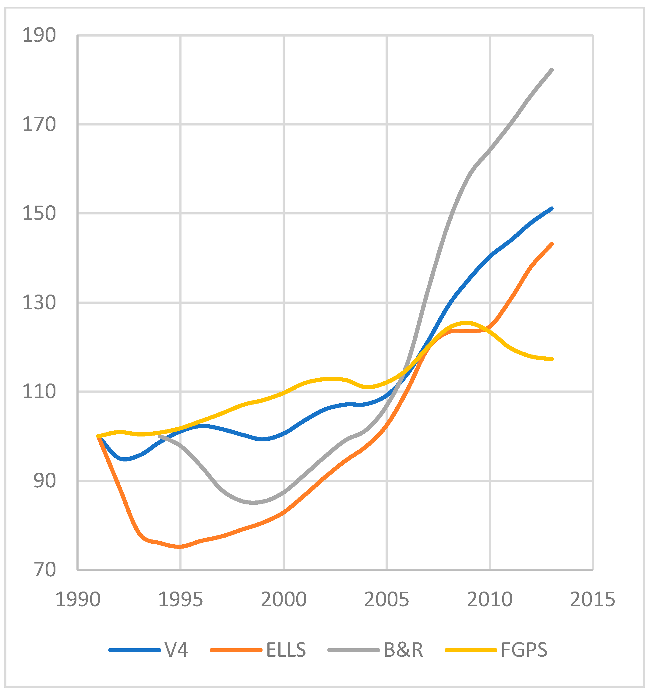
In addition to studying average exponential growth rates over various periods, examining year-to-year changes in income may also be of some interest. Figure 1 presents the catch-up index for V4, ELLS, and FGPS for 1991 to 2014 and for B&R for 1994–2014. The income of V4 (“old” ex-socialist countries) does not fall. On the other hand, ELLS (“new” ex-socialist countries) sharply fall behind (the US) for about three years and then start gradual recovery. (The descriptive data in Figure 1 shows that these countries’ incomes did not rise much faster than the US’s pre-2004 or pre-2007 and does not show an anticipation effect. Rather, the sharp boost in their income comes in 2005.) This paper suggests the explanation to be that initial institutional conditions of “new” ex-socialist countries were worse than those of the “old”—the former had the additional burden of creating a completely new governance structure and economic relationships.
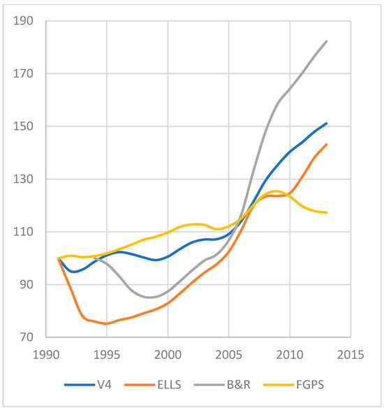
Figure 1.
The catch-up index for V4, ELLS, and FGPS, 1991–2014, and for B&R, 1994–2014.
The vertical axis of Figure 1 measures the catch-up index (Scale: 1” = 40). FGPS stands for France, Greece, Portugal and Spain, V4 for the Visegrád Four, Czechia, Hungary, Poland, and Slovakia, ELLS for Estonia, Latvia, Lithuania and Slovenia, and B&R for Bulgaria and Romania. The catch-up index is the index of income ratios to the US with the initial year’s income ratio equal to 100 for all groups. The actual income ratios for the four groups for the start year were 0.37, 0.37, 0.25, and 0.53, respectively.
5. DID Estimation Results, Discussion, and Institutional Changes Adopted
Section 5.1 presents the DID estimation results of EU accession, while Section 5.2 describes the institutional changes adopted by the accession countries in the process of EU accession.
5.1. DID Estimation Results and Discussion
Stata’s (Stata/BE 18) DID Regression command is used to estimate Equation (1) and to test the associated null hypothesis that pre-treatment trends are parallel. For V4 and ELLS, the panels consist of eight countries each, consisting of four treatment countries, V4 or ELLS, and four control countries, FGPS. DID estimation results for these groups of countries are presented in Table 2. They satisfy the pre-treatment parallel trends F test (null hypothesis: pre-treatment trends are parallel), and the positive treatment coefficient is statistically significant. The results for the 1991–2014 period are presented in columns with 192 observations in Table 2 and assume that the EU accession occurred on 1 January 2014. Since all these countries joined the EU in the middle of 2004 (on 1 May 2004), columns with 184 observations show the estimation results with observations for 2014 deleted for all countries, treatment, and control. The positive treatment effect for both V4 and ELLS increases. That is, a clearer separation of post-accession and pre-accession periods increases the effect on incomes of joining the EU, giving further support to our hypothesis.
Table 2.
DID est. effect on income of EU acc. with FGPS as control group and V4 and ELLS as treatment group.
The income ratio in 2003 was 0.378 for V4 and 0.351 for ELLS. The magnitude of the average ATET is an increase in income ratio of 0.042 for V4 and 0.079 for ELLS. That translates to a post-accession increase in income of V4 during 2005–2014 by 11% over the control countries, and of ELLS by 23%, due to institutional integration cum improvement of V4 and ELLS as they joined the EU.
The DID estimation results for B&R are presented in Table 3. Now, the panel consists of six countries, two treatment countries and the same four control countries, FGPS. Again, the parallel pre-treatment trends test is satisfied, and the positive treatment coefficient is statistically significant. Now, to have a clearer separation of post-accession and pre-accession periods, the observations for 2006 and 2007 for all six countries are deleted. The results, in Table 3’s second column, show that the positive effect of treatment again increases.
Table 3.
DID est. effect on income of EU acc. with FGPS as control group and B&R as treatment group.
The income ratio in 2005 was 0.22 for B&R. The magnitude of the average ATET is an increase in income ratio by 0.074 for B&R. That translates to a post-accession increase in income of B&R by 33% over the control countries due to their institutional integration cum improvement as they joined the EU.
Graphical diagnostics for parallel pre-treatment trends for V4, ELLS, and B&R are presented in Appendix A, Figure A1, Figure A2, and Figure A3, respectively.
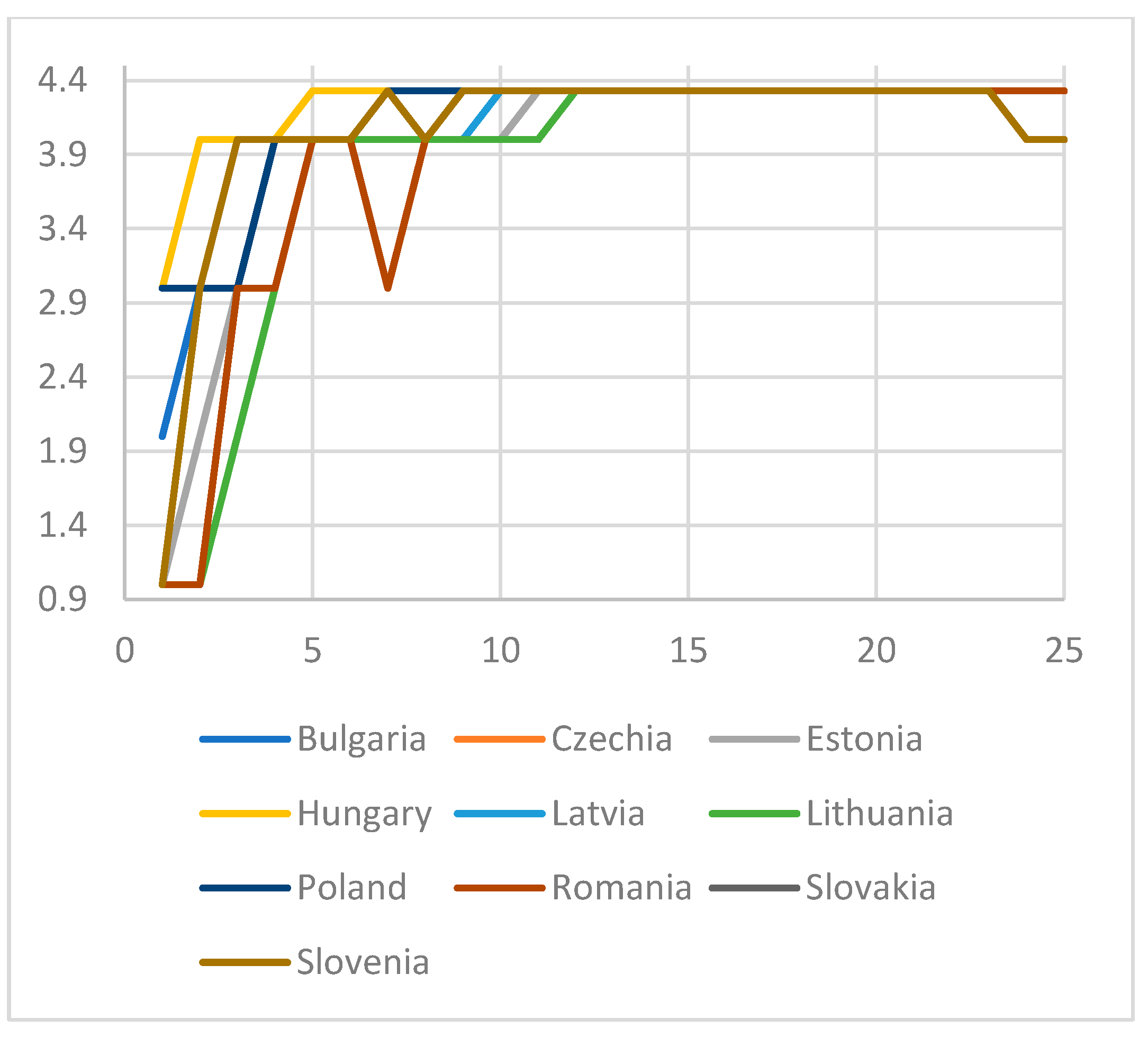
The above estimation shows that joining the EU boosted the income of all three groups of countries. Analyzing growth rates in Table 1 shows that FGPS were growing faster than V4 and ELLS before the latter groups of countries joined the EU. Then, both the (i) higher growth of V4 and B&R and (ii) all growth of ELLS from 1990 (since their income fell from 1991 to 2003) are entirely explained by the spurt in growth after they joined the EU. All ten of these countries had introduced not just trade and foreign exchange system openness but also domestic neo-liberal economic policies and democracy in the early 1990s (see Appendix A, Figure A4), and all other than Slovakia had adopted FDI promotion strategies (see Bohle, 2018).
EBRD has rated all the transition (or reform) economic indicators for all ex-socialist countries for the period since 1989. Its description and what a country must do to progress from the lowest level or little progress (1.00) to the maximum (attainment of advanced industrial economy standards or 4.33) score—where the scores are not cardinal and it is increasingly difficult to achieve a higher score (see Raiser et al., 2001)—in each is described at https://www.ebrd.com/home/what-we-do/office-of-the-chief-economist/transition-indicators-methodology-1989-2014.html#. The EU10 countries had attained the maximum score for all indicators by the late 1990s. Rather than adopting economic reforms after joining the EU, it was improving their institutions that was new.
While highlighting that the quality of institutions is even more important in the civil law countries that all Central and East European countries are, Kowalewski and Rybinski (2011) complain that they (i) had to follow the EU’s environmental policies, for example, the CO2 policy, that the USA and BRICs do not and (ii) report that they (except Estonia) had to pass an avalanche of new laws/regulations and create new bureaucratic processes pre-accession that burdened the state. These and Maastricht debt and deficit criteria burdens must be counter-balanced by the EU’s Cohesion and Structural funds, which the new member states received from the EU (which were as high as 4 percent of the GDP). See Kowalewski and Rybinski (2011) and Bohle (2018).
As stated above, the closest papers to our study are those of Campos et al. (2019) and Cieślik and Turgut (2021). We compare in Table 4 this study to Campos et al. (2019) and Cieślik and Turgut (2021) for the question all three papers study, namely, the effect of 2004 accession on income and growth.
Table 4.
Comparison to Campos et al. (2019) and Cieślik and Turgut (2021).
As discussed above, Campos et al. (2019) find mixed effects, Cieślik and Turgut (2021) find stronger effects from 2007, and this paper finds strong effects from the year of EU accession. It finds the effect is stronger for “new” ex-socialist countries, ELLS, and countries with lower initial levels of institutions, Bulgaria and Romania, which joined the EU in 2007. As shown below, estimating the post-accession periods separately from the pre-accession, for all three groups, it finds that it is human capital that drives the positive results.
Some of the limitations of our analysis may be noted. Institutional-integration anchors started even before the official accession date. Of course, the accession itself was a big supply-and-demand shock to the new entrants and caused changes in institutions, but changes in institutions constitute a staggered and complex process likely to take some years to accomplish. In fact, the EU was quite vigilant for the Eastern enlargement—due to vast institutional differences, this was the only enlargement for which the EU created a surveillance mechanism. However, in both the estimation methods, TWFE DID and SC, the treatment is binary. This paper has tried to overcome this problem in our DID estimation by deleting the middle year(s) from estimation. However, it is unlikely that it has eliminated all institutional changes in the years that remain. The only consolation is that the estimated ATET then most likely understates the true effect.
5.2. Institutional Changes Adopted to Obtain EU Accession
The following may be noted as an example of the institutional changes the EU10 adopted to obtain EU membership: the Bulgarian legislature, in January 2006, adopted reforms generated by the public–private initiative, Coalition 2000, in the areas of “political level corruption, VAT fraud, a stricter system of implementation monitoring, a stronger mandate for the oversight government commission, and in limiting/lifting the immunity of parliament members and magistrates under specified conditions.” For further examples and for other countries, see Phinnemore (2006), Pond (2006), Streimann (2007), Kesteris and Plamse (2007), Telicka and Bartak (2007), Lusman (2014), and the European Commission, Cooperation, and Verification Mechanism for Bulgaria and Romania (European Commission, 2023). V4, ELLS, and B&R implemented a variety of very detailed policies over many years to join the EU.
Comparing the ATET for the three groups of countries, the effect is stronger for ELLS and B&R. One explanation can be that both ELLS and B&R had a greater scope of improvement in their institutions than V4. Based on perceptions of households, businesses, and citizens, the World Bank has compiled a database of six indicators of quality of governance in over 200 economies for the period since 1996. The six indicators are voice and accountability (voice in selecting the government and freedom of expression, association, and media), political stability and absence of (political) violence/terrorism, government effectiveness (quality of public services, policy formulation and implementation, and absence of political interference in civil service), regulatory quality (sound regulations that permit and promote the private sector), rule of law (quality of contract enforcement, property rights, police, and courts), and control of corruption (public power not exercised for private gain and no elite/private interest capture of the state).
The average of the last four indicators—government effectiveness, regulatory quality, rule of law, and control of corruption—is used to indicate the quality of institutions particularly relevant for economic activity. These data are depicted in Figure 2 for the three groups of countries. They show that (i) B&R had the lowest level of institutions, and (ii) the deterioration in the institutions in ELLS was also in the late 1990s. Using the average of all six indicators does not change these conclusions. Further, in response to concerns expressed by stakeholders, the World Bank is implementing changes to strengthen its Governance Indicators database and has adopted a usage advisory for 2024. See https://www.worldbank.org/en/publication/worldwide-governance-indicators/usage-advisory accessed 19 March 2025. (The other possible institutional variables in this context are the Index of Economic Freedom, developed by the Heritage Foundation, a private think-tank, for 1995 and later, and the Ease of Doing Business by the World Bank. Historical data on the former is not available for download, and the latter has been discontinued with effect since 16 September 2021 due to data problems for some earlier years. See https://www.worldbank.org/en/news/statement/2021/09/16/world-bank-group-to-discontinue-doing-business-report accessed on 2 February 2023.) It is most likely due to these factors that B&R and ELLS had a sharp improvement in their institutions around their EU accession year, yielding a stronger ATET.
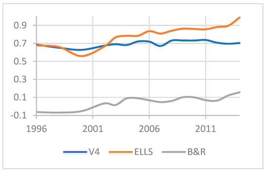
Figure 2.
Governance Indicators, V4, ELLS, B&R, 1996–2014.
6. Proximate Factor(s) Results and Discussion
Now, the paper examines whether the positive ATET are due to a specific proximate growth factor. To answer that question, it estimates Equation (3) by panel regression separately for the two periods—post-EU accession and pre-accession—for the three country groups in turn. Results are presented in Table 5. The number of observations for the two periods are 52 and 34, respectively, for V4 and ELLS, and 20 and 16 for B&R. For V4, all the variables are statistically significant at the 1 percent level in the two periods. TFP’s contribution to income is higher in the post-EU accession, and that of physical capital is lower. The dramatic difference is on the effect of human capital. From the coefficient with the wrong sign in the pre-EU accession period, it changes to have (the expected) positive effect in the post-EU accession period.
Table 5.
Growth factors for EU accession countries.
The differences in post-accession versus pre-accession effects of physical capital and TFP cannot be easily summarized for ELLS and B&R (although TFP’s role for ELLS increases post-accession). But the comparison of the effects of human capital yields the same result as for V4—the sign of the effect changes from negative to positive (and for B&R, the effect also becomes statistically significant in that it was not pre-accession). For all three country groups, it is human capital that stands out as the main difference between the effects of estimating (3) for the two periods. It is human capital that primarily explains the spurt in growth following EU accession.
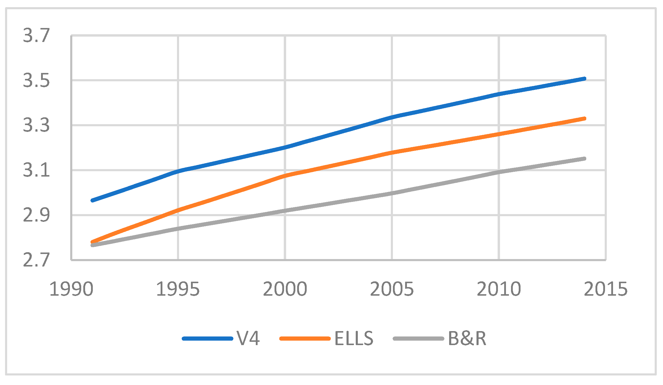
Figure 3 depicts the average human capital of the three groups of countries for the 1991 to 2014 period. Human capital grows linearly for all three groups—it is not growing faster post-accession. Yet, it is the only proximate factor that is statistically significant for all three groups of countries post-accession. Kutan and Yigit (2007) find that both improved productivity and physical capital accumulation explain the higher post-accession growth of the last five members that joined the EU and increased its membership to 15, namely, Spain, Portugal, Austria, Finland, and Sweden. For the EU10, it is human capital, instead. Data on the institutional quality of Spain, Portugal, Austria, Finland, and Sweden or of other countries in the EU15 when these countries joined the EU is not available. But it is very likely the institutional quality of Spain, Portugal, Austria, Finland, and Sweden was closer to that of the rest of the EU15 when they joined the EU as compared to that of the EU10 when they joined the EU15. When institutional quality was almost the same, EU accession boosted the income of the joiners via TFP and physical capital; when it was different, it boosted it via human capital.
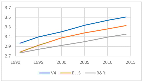
Figure 3.
Human capital, V4, ELLS, and B&R, 1991–2014.
The above analysis shows human capital is the most important factor explaining both (i) higher growth of V4 and (ii) all growth of ELLS following EU accession. EU norms reduced (if not eliminated) the divergence of human capital’s output and income to others, permitted it to work in transparent networks, and increased its incentive to work. The new access to the EU’s Social Fund (ESF; see Kechagia & Kyriazi, 2021, for its description) fostered the adaptability of workers and enhanced their access to employment and labor markets. The result emphasizing human capital is consistent with the work of Marin (2010), who, after examining in detail German and Austrian investment undertakings in Eastern Europe in 2010, finds that these countries relocated their skilled jobs to cheaper East European locations. East European labor did not acquire job skills on EU accession—these countries’ human capital, measured by, say, average years of schooling, was better at transition than the OECD average (and did not go down in the 1990s). See Barro and Lee (2001). Campos and Coricelli (2002) highlight Central and East European countries’ pre-transition human capital development by suggesting that just comparing their per capita income to that of the EU15 at transition ignores the efforts these countries devoted to improving education and health during socialism. Labor, with the same skills they had for decades, created more value with the right institutions.
Glaeser et al. (2004, p. 5) (as noted above) find that “initial levels of constraints on the executive [that they identify as good institutions] do not predict subsequent growth, whereas initial levels of human capital continue to be strong predictors.” In our view, the identification of institutions as constraints on the head of the state (for example, whether a country has an unconstrained dictator) or on the government in general is narrow. In addition to “a set of rules, compliance procedures,” institutions are also “moral and ethical behavioral norms” that “constrain the behavior of individuals.” (North, 1981, pp. 201–202). That is, institutions include meso- and micro-institutions. The collapse of communism meant a dilution of constraints at all levels (state, city, enterprise/organization, and individual) and the emergence of opaque business networks. It created poor institutions that did not permit skilled human capital to contribute to growth. Institutional changes with EU accession improved these poor institutions—externally imposed constraints by the EU replaced these opaque networks by transparent networks.
Erosa et al. (2010) construct a model of heterogeneous individuals to quantitatively compare the effects of TFP and human capital on cross-country income differences. They find human capital amplifies the effect of TFP differences by about fourfold. Hanushek et al. (2017), while finding results to be insensitive to differences in price levels across states (available since 2008), show that differences in human capital account for 20 to 30 percent of differences in per capita GDP of states within the US. This paper finds a far greater role of human capital in situations when institutions change and improve.
The paper uses per capita income as the dependent variable for both the TWFE DID model and the neo-classical growth model. Technically, for the neo-classical growth model, the dependable variable is per worker output. The paper uses per capita output for the neo-classical growth model as well to have the same dependable variable for both the estimations. Further, it assumes the same proportion of the population is employed in the EU10 countries both before EU accession and after it. However, this assumption may not be true.
7. Conclusions
The broader implication of this paper is that good institutions are crucial in middle- or high-income countries, as well. Fernald et al. (2017) ascribe slower post-Great Recession recovery in the US to slower growth of TFP, and Hanushek et al. (2017) find human capital accounts for 20 to 30 percent of differences in the per capita GDP of states within the US. This paper finds a greater role of human capital on growth than either of these studies. It analyzes its role when institutions can change, and, like Rossi (2020), finds human capital and institutions to be complementary.
The policy implications of this study are twofold. First, this study highlights the variables that pre-dispose an economy’s institutional quality to improve as a result of regional economic integration. These are a long period (over many decades) of not having been capitalist democracies, initial low institution quality levels, burdened with creating institutions due to emerging as independent countries, say, at post-colonial independence, and when the existing members of the integrated entity condition membership of aspirants to an upgrade in their institutions. The EU10’s accession to the EU is a prime example of countries/regions meeting one or more of these conditions.
Second, this study recommends that institutions ought to be improved to permit factors of production to create value they are capable of. Human capital in PWT is measured based on years of schooling. However, comparative research based on results from TIMMS and later PISA has demonstrated that the quality of a year of schooling differs substantially across countries. See Hanushek and Kimko (2000). Directions for future research are to update the analysis when quality-adjusted data on human capital are available.
Funding
This research received no external funding.
Institutional Review Board Statement
Not applicable.
Informed Consent Statement
Not applicable.
Data Availability Statement
The data that support the findings of this study are openly available in Penn World Table version 9.0 at http://www.rug.nl/ggdc/productivity/pwt accessed on 2 January 2021.
Conflicts of Interest
The author declares no conflicts of interest.
Appendix A
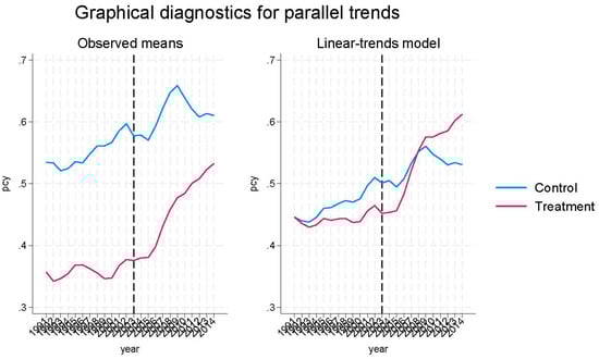
Figure A1.
Graphical diagnostics for parallel trends for V4.
Figure A1.
Graphical diagnostics for parallel trends for V4.
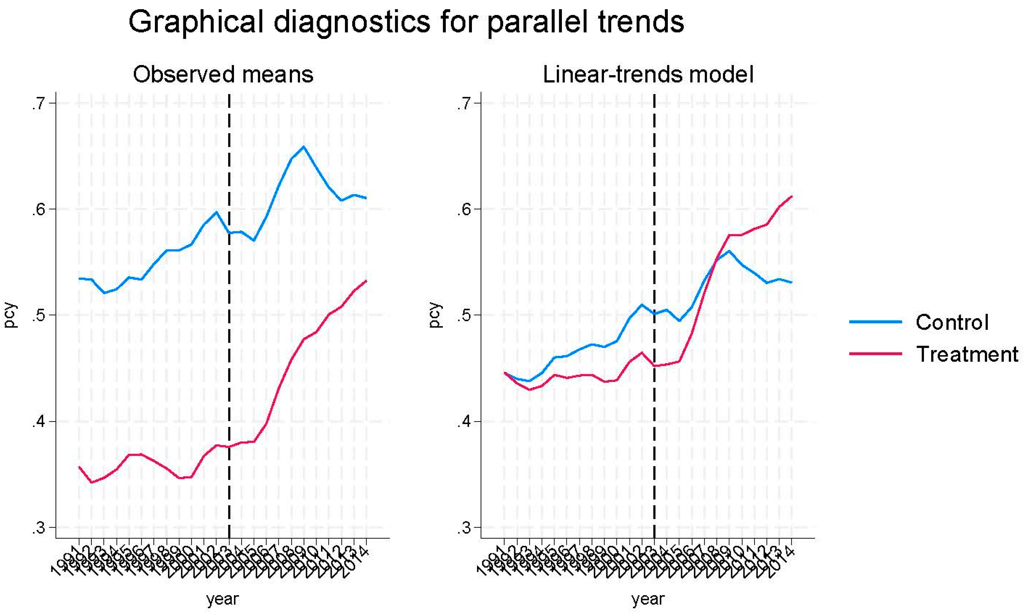
Figure A2.
Graphical diagnostics for parallel trends for ELLS.
Figure A2.
Graphical diagnostics for parallel trends for ELLS.
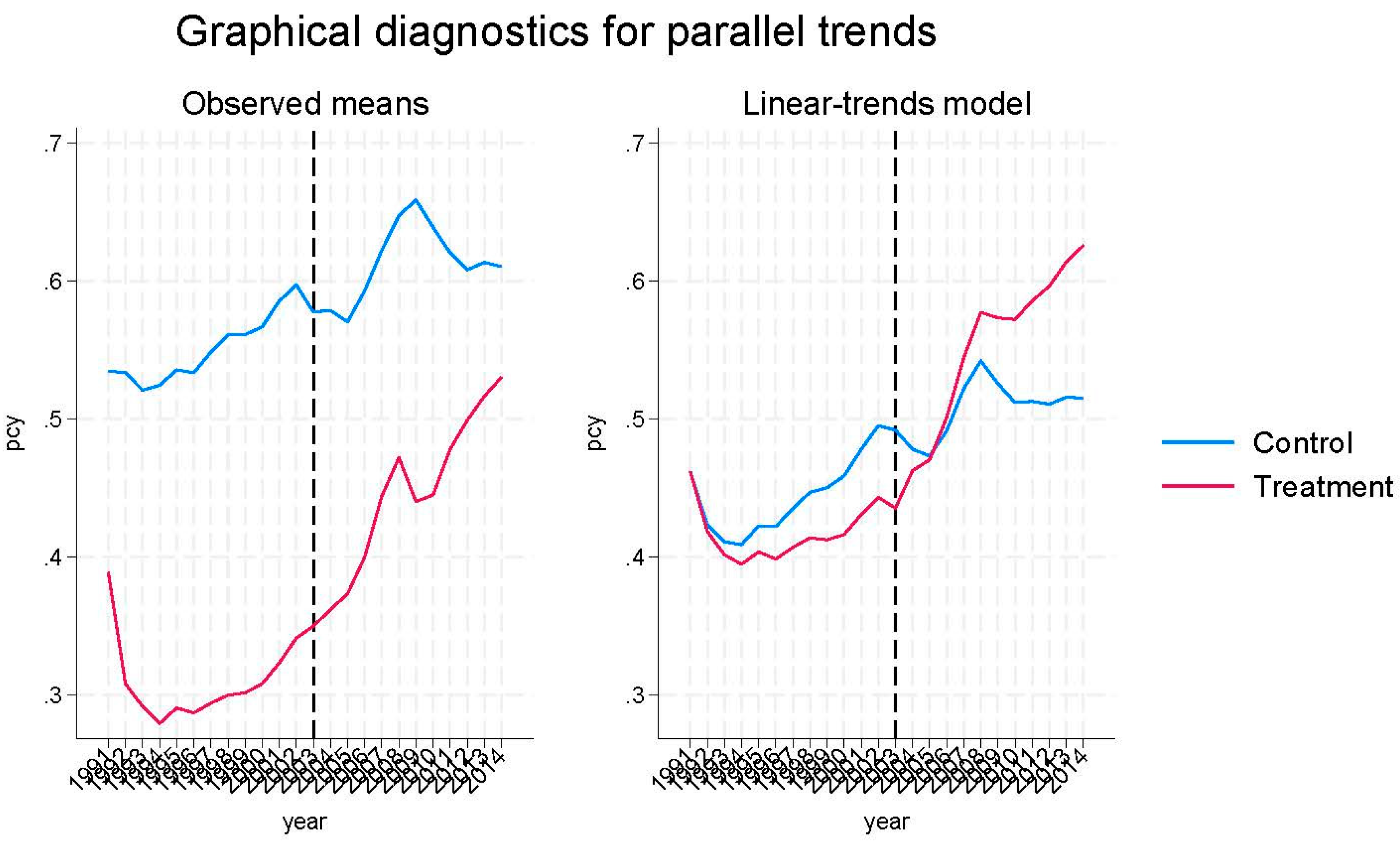
Figure A3.
Graphical diagnostics for parallel trends for B&R.
Figure A3.
Graphical diagnostics for parallel trends for B&R.
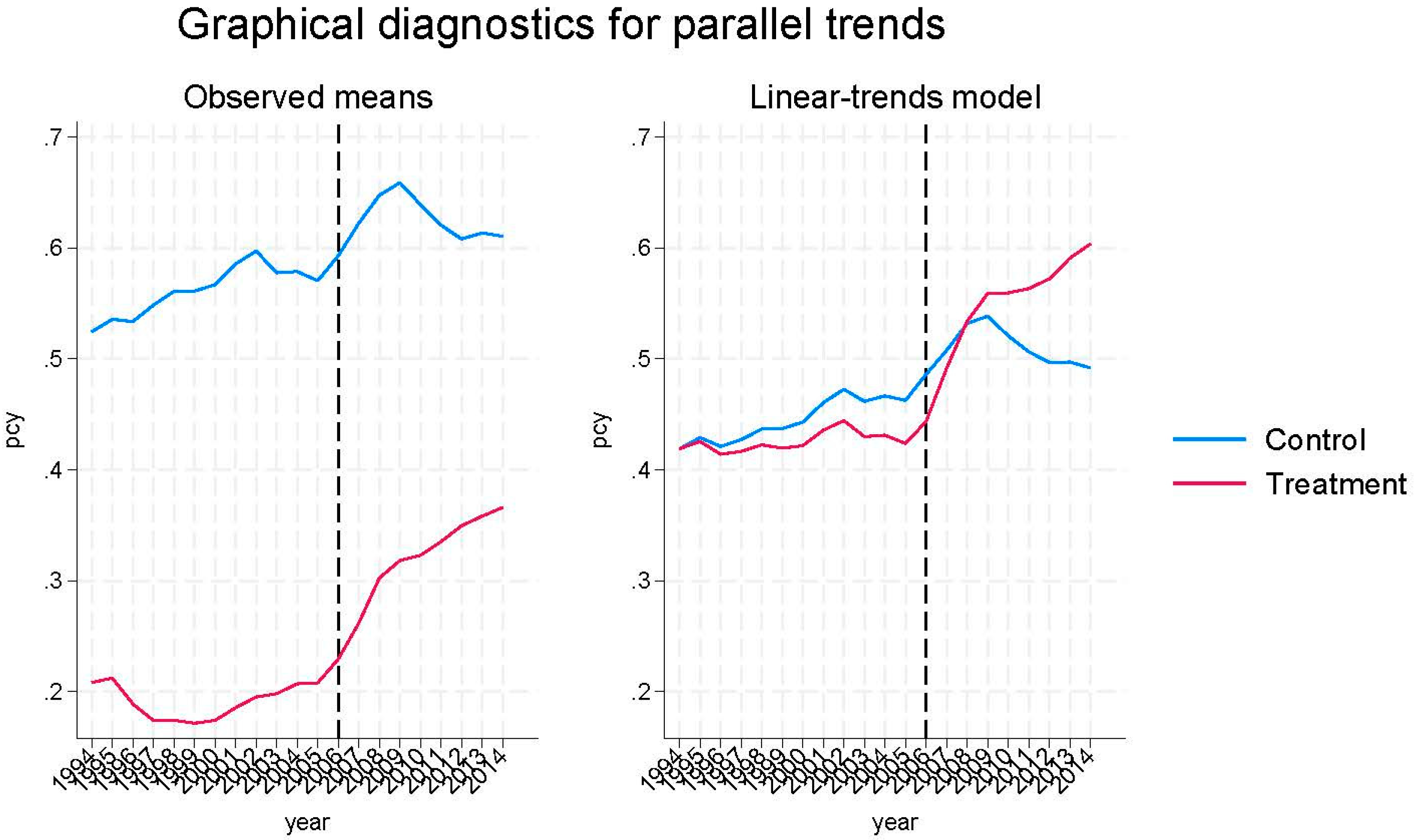
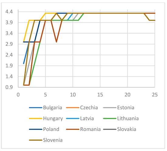
Figure A4.
Trade and foreign exchange transition indicator, 1990–2014; EU10 countries.
Figure A4.
Trade and foreign exchange transition indicator, 1990–2014; EU10 countries.
References
- Abadie, A., Diamond, A., & Hainmueller, J. (2010). Synthetic control methods for comparative case studies: Estimating the effect of California’s tobacco control program. Journal of the American Statistical Association, 105(490), 493–505. [Google Scholar] [CrossRef]
- Abadie, A., Diamond, A., & Hainmueller, J. (2015). Comparative politics and the synthetic control method. American Journal of Political Science, 59(2), 495–510. [Google Scholar] [CrossRef]
- Abadie, A., & Gardeazabal, J. (2003). The economic costs of conflict: A case study of the Basque country. American Economic Review, 93(1), 113–132. [Google Scholar] [CrossRef]
- Acemoglu, D., Johnson, S., & Robinson, J. A. (2005). Institutions as a fundamental cause of long-run growth. In P. Aghion, & S. Durlauf (Eds.), Handbook of economic growth (pp. 385–472). Elsevier. [Google Scholar]
- Alfaro, L., Kalemli-Ozcan, S., & Volosovych, V. (2008). Why doesn’t capital flow from rich to poor countries? An empirical investigation. Review of Economics and Statistics, 90, 347–368. [Google Scholar] [CrossRef]
- An, W., & Winship, C. (2017). Causal inference in panel data with application to estimating race-of-interviewer effects in the general social survey. Sociological Methods and Research, 46, 68–102. [Google Scholar] [CrossRef]
- Angrist, J., & Pischke, J. (2010). The credibility revolution in empirical economics: How better research design is taking the con out of econometrics. Journal of Economic Perspectives, 24(2), 3–30. [Google Scholar] [CrossRef]
- Arkhangelsky, D., Athey, S., Hirshberg, D. A., Imbens, G. W., & Wager, S. (2021). Synthetic difference-in-differences. American Economic Review, 111(12), 4088–4118. [Google Scholar] [CrossRef]
- Ashenfelter, O., & Card, D. (1985). Using the longitudinal structure of earnings to estimate the effect of training programs. Review of Economics and Statistics, 67(4), 648–660. [Google Scholar] [CrossRef]
- Babecký, J., & Campos, N. F. (2011). Does reform work? An econometric survey of the reform-growth puzzle. Journal of Comparative Economics, 39(2), 140–158. [Google Scholar] [CrossRef]
- Baker, A. C., Larcher, D. F., & Wong, C. C. Y. (2022). How much should we trust staggered difference-in-differences estimates? Journal of Financial Economics, 144(2), 370–395. [Google Scholar] [CrossRef]
- Barro, R., & Lee, J.-W. (2001). International data on educational attainment: Updates and implications. Oxford Economic Papers, 53(3), 541–563. [Google Scholar] [CrossRef]
- Barro, R. J., & Lee, J. W. (2013). A new data set of educational attainment in the world, 1950–2010. Journal of Growth Economics, 104, 184–198. [Google Scholar] [CrossRef]
- Beck, T., & Laeven, L. (2006). Institution building and growth in transition economies. Journal of Economic Growth, 11(2), 157–186. [Google Scholar] [CrossRef]
- Becker, G. (1962). Investment in human capital. Journal of Political Economy, 70(5), 9–49. [Google Scholar] [CrossRef]
- Bohle, D. (2018). European integration, capitalist diversity and crises trajectories on Europe’s eastern periphery. New Political Economy, 23(2), 239–253. [Google Scholar] [CrossRef]
- Boltho, A., & Eichengreen, B. (2008). The economic impact of European integration [CEPR discussion paper No. 6820]. CEPR. [Google Scholar]
- Callaway, B., & Sant’Anna, P. H. C. (2021). Difference-in-differences with multiple time periods and an application on the minimum wage and employment. Journal Econometrics, 225, 200–230. [Google Scholar] [CrossRef]
- Campos, N. F., & Coricelli, A. (2002). Growth in transition: What we know, what we don’t, and what we should. Journal of Economic Literature, 40(3), 793–836. [Google Scholar] [CrossRef]
- Campos, N. F., Coricelli, F., & Franceschi, E. (2022). Institutional integration and productivity growth: Evidence from the 1995 enlargement of the European union. European Economic Review, 142, 104014. [Google Scholar] [CrossRef]
- Campos, N. F., Coricelli, F., & Moretti, L. (2019). Institutional integration and economic growth in Europe. Journal of Monetary Economics, 103, 88–104. [Google Scholar] [CrossRef]
- Cieślik, A., & Turgut, M. B. (2021). Estimating the growth effects of 2004 eastern enlargement of the European union. Journal of Risk and Financial Management, 14(3), 128. [Google Scholar] [CrossRef]
- Cohen, D., & Leker, L. (2014). Health and education: Another look with the proper data [CEPR discussion paper No. DP9940]. CEPR. [Google Scholar]
- Cohen, D., & Soto, M. (2007). Growth and human capital: Good data, good results. Journal of Economic Growth, 12(1), 51–76. [Google Scholar] [CrossRef]
- Currie, J., Kleven, H., & Zwiers, E. (2020). Technology and big data are changing economics: Mining text to track methods. AEA Papers and Proceedings, 110, 42–48. [Google Scholar] [CrossRef]
- Dehejia, V. H. (1996). Shock therapy vs. gradualism: A neoclassical perspective. Eastern Economic Journal, 22(4), 425–431. [Google Scholar]
- Ehrlich, I., Cook, A., & Yin, Y. (2018). What accounts for the us ascendancy to economic superpower by the early twentieth century? The morrill act–human capital hypothesis. Journal of Human Capital, 12(2), 233–281. [Google Scholar] [CrossRef]
- Erosa, A., Koreshkova, T., & Restuccia, D. (2010). How important is human capital? A quantitative theory assessment of world income inequality. Review of Economic Studies, 77(4), 1421–1449. [Google Scholar] [CrossRef]
- European Commission. (2023). Rule of law: Commission formally closes the cooperation and verification mechanism for Bulgaria and Romania. Available online: https://ec.europa.eu/commission/presscorner/detail/pt/ip_23_4456 (accessed on 12 June 2025).
- Felbermayr, G., Gröschl, J., & Steinwachs, T. (2016). The trade effect of border controls: Evidence from the European Schengen agreement [Ifo working paper No. 213]. Ifo Institute. [Google Scholar]
- Fernald, J. G., Hall, R. E., Stock, J. H., & Watson, M. W. (2017). The disappointing recovery of output after 2009 (pp. 1–58). [Brookings papers on economic activity]. NBER. [Google Scholar]
- Fuchs-Schündeln, N., & Hassan, T. A. (2015). Natural experiments in macroeconomics [NBER working paper 21228]. NBER. [Google Scholar]
- Glaeser, E., La Porta, R., Lopez-de-Silanes, F., & Shleifer, A. (2004). Do institutions cause growth? Journal of Economic Growth, 9, 271–303. [Google Scholar] [CrossRef]
- Grier, K. B., & Grier, R. M. (2021). The Washington consensus works: Causal effects of reform, 1970–2015. Journal of Comparative Economics, 49(1), 59–72. [Google Scholar] [CrossRef]
- Hall, R. E., & Jones, C. I. (1999). Why do some countries produce so much more output per worker than others. Quarterly Journal of Economics, 114, 83–116. [Google Scholar] [CrossRef]
- Hanushek, E. A., & Kimko, D. D. (2000). Schooling, labor force quality and the growth of nations. American Economic Review, 90(5), 1184–1208. [Google Scholar] [CrossRef]
- Hanushek, E. A., Ruhose, J., & Woessmann, L. (2017). Knowledge capital and aggregate income differences: Growth accounting for U.S. states. American Economic Journal: Macroeconomics, 9(4), 184–224. [Google Scholar]
- Hoen, H. W. (1996). Shock versus gradualism in central Europe reconsidered. Comparative Economic Studies, 38(1), 1–20. [Google Scholar] [CrossRef]
- Inklaar, R., & Timmer, M. P. (2013). Capital, labor and TFP in PWT 8.0. Groningen Growth and Development Centre, University of Groningen. [Google Scholar]
- Johnson, S., Kaufmann, D., McMillan, J., & Woodruff, C. (2000). Why do firms hide? Bribes and unofficial activity after communism. Journal of Public Economics, 76(3), 495–520. [Google Scholar] [CrossRef]
- Jones, B. F., & Olken, B. A. (2008). The anatomy of start-stop growth. Review of Economics and Statistics, 90(3), 582–587. [Google Scholar] [CrossRef]
- Jones, C. J., & Romer, P. M. (2012). New Kaldor facts: Ideas, institutions, population, and human capital. American Economic Journal: Macroeconomics 2, 224–245. [Google Scholar]
- Kant, C. (2019). Income convergence and the catch-up index. The North American Journal of Economics and Finance, 48, 613–627. [Google Scholar] [CrossRef]
- Kantorowicz, J., & Spruk, R. (2024). Using synthetic control method to estimate the growth effects of economic liberalization: Evidence from transition economies. World Economy, 47(6), 2332–2360. [Google Scholar] [CrossRef]
- Kechagia, A., & Kyriazi, F. (2021). Structural funds and regional economic growth: The Greek experience. Review of Economic Analysis, 13, 501–528. [Google Scholar]
- Kesteris, A., & Plamse, K. (2007). The accession of Latvia to the EU. In G. Vassiliou (Ed.), The accession story: EU From 15 to 25 countries. OUP. [Google Scholar]
- Knack, S., & Keefer, P. (1997). Does social capital have an economic payoff? A cross-country investigation. Quarterly Journal of Economics, 112, 1251–1288. [Google Scholar] [CrossRef]
- Kowalewski, O., & Rybinski, K. (2011). The hidden transformation: The changing role of the state after the collapse of communism in central and eastern Europe. Oxford Review of Economic Policy, 27(4), 634–657. [Google Scholar] [CrossRef]
- Kutan, A. M., & Yigit, T. M. (2007). European integration, productivity growth and real convergence. European Economic Review, 51(6), 1370–1395. [Google Scholar] [CrossRef]
- Lawrence, R. Z. (1996). Regionalism, multilateralism, and deeper integration. Brookings Institution Press. [Google Scholar]
- Lucas, R. E., Jr. (1990). Why doesn’t capital flow from rich to poor countries? American Economic Review 80, 92–96. [Google Scholar]
- Lusman, I. (2014). European union accession conditionality and human rights in Romania. In Children’s rights, eastern enlargement and the EU human rights regime (Chapter 2). Manchester University Press. [Google Scholar]
- Marin, D. (2010). The opening up of eastern Europe at 20-jobs, skills, and ‘reverse maquiladoras’ in Austria and Germany. The Quarterly Journal of Economics, 14(1), 85–120. [Google Scholar]
- Mauro, P. (1995). Corruption and growth. Quarterly Journal of Economics, 110, 681–712. [Google Scholar] [CrossRef]
- Melki, M. (2022). Inequality and investment: The role of institutions. Economic Modelling, 108, 105736. [Google Scholar] [CrossRef]
- Morck, R., Wolfenzon, D., & Yeung, B. (2005). Corporate governance, economic entrenchment and growth. Journal of Economic Literature, 43, 655–720. [Google Scholar] [CrossRef]
- North, D. C. (1981). Structure and change in economic history. Norton. [Google Scholar]
- Nunn, N. (2014). Historical growth. In S. N. Durlauf, & A. Phillipe (Eds.), Handbook of economic growth (Vol. 2A). Elsevier B.V. [Google Scholar]
- Papaioannou, E. (2009). What drives international financial flows? Politics, institutions and other determinants. Journal of Development Economics, 88, 269–281. [Google Scholar] [CrossRef]
- Papaioannou, E., & Siourounis, G. (2008). Democratization and growth. Economic Journal, 118(532), 1520–1551. [Google Scholar] [CrossRef]
- Persson, T., & Tabellini, G. (2008). The growth effect of democracy: Is it heterogeneous and how can it be estimated? In E. Helpman (Ed.), Institutions and economic performance (Chapter 13). Harvard University Press. [Google Scholar]
- Phinnemore, D. (2006). Two more for the club. The World Today, 62(10), 22–23. [Google Scholar]
- Pond, E. (2006). Reinventing Bulgaria. In Endgame in the Balkans: Regime change, European style (pp. 39–67). Chapter 2. Brookings Institution Press. [Google Scholar]
- Psacharopoulos, G. (1994). Returns to investment in education: A global update. World Growth, 22(9), 1325–1343. [Google Scholar] [CrossRef]
- Raiser, M., Diommaso, M., & Weeks, M. (2001). the measurement and determinants of institutional change: Evidence from transitional economies. [Working papers No. 60]. EBRD. [Google Scholar]
- Rodrik, D. (Ed.). (2003). Search of prosperity: Analytic narratives on economic growth. Princeton University Press. [Google Scholar]
- Rodrik, D., Subramanian, A., & Trebbi, F. (2004). Institutions rule: The primacy of institutions over geography and integration in economic development. Journal of Economic Growth, 9, 131–165. [Google Scholar] [CrossRef]
- Rodrik, D., & Wacziarg, R. (2005). Do democratic transitions produce bad outcomes? American Economic Review, 95(2), 50–55. [Google Scholar] [CrossRef]
- Rosenberg, N., & Birdzell, L. E. (1996). How the west grew rich: The economic transformation of the western world. Basic Books. [Google Scholar]
- Rossi, F. (2020). Human capital and macroeconomic development: A review of the evidence. The World Bank Research Observer, 35(2), 227–262. [Google Scholar] [CrossRef]
- Schultz, T. W. (1960). Capital formation by education. Journal of Political Economy, 68(6), 571–583. [Google Scholar] [CrossRef]
- Smith, A. (1776). The wealth of nations. Random House. [Google Scholar]
- Solow, R. (1956). A Contribution to the theory of economic growth. Quarterly Journal of Economics, 70(1), 65–94. [Google Scholar] [CrossRef]
- Streimann, A. (2007). The accession of Estonia to the EU. In G. Vassiliou (Ed.), The accession story: The EU from 15 to 25 countries. OUP Oxford. [Google Scholar]
- Telicka, P., & Bartak, K. (2007). The accession of the Czech Republic to the EU. In G. Vassiliou (Ed.), The accession story: The EU from 15 to 25 countries. OUP Oxford. [Google Scholar]
- Van Ees, H., & Bachmann, R. (2006). Transition economies and trust building: A network perspective on EU enlargement. Cambridge Journal of Economics, 30(6), 923–939. [Google Scholar] [CrossRef]
- World Bank. (2024). Worldwide governance indicators. Available online: https://www.worldbank.org/en/publication/worldwide-governance-indicators (accessed on 25 July 2024).

Disclaimer/Publisher’s Note: The statements, opinions and data contained in all publications are solely those of the individual author(s) and contributor(s) and not of MDPI and/or the editor(s). MDPI and/or the editor(s) disclaim responsibility for any injury to people or property resulting from any ideas, methods, instructions or products referred to in the content. |
© 2025 by the author. Licensee MDPI, Basel, Switzerland. This article is an open access article distributed under the terms and conditions of the Creative Commons Attribution (CC BY) license (https://creativecommons.org/licenses/by/4.0/).