External and Internal Shocks and the Movement of Palm Oil Price: SVAR Evidence from Malaysia

Abstract

Movements in palm oil price give important signals to various stakeholders of the palm oil industry in Malaysia. Thus, understanding external and internal factors that may affect the palm oil price is vital to the industry players for sustainability of their activities. This study investigates relative importance of external and internal shocks on the movement of palm oil price in Malaysia. Employing a structural vector autoregressive (SVAR) model on quarterly data from 1990 to 2019, the findings reveal that external shocks are more dominant in affecting the palm oil price. Shocks to the crude oil price, the prices of substitution goods (soybeans oil, rapeseed oil, and sunflower oil), the world palm oil price, and foreign income significantly affect the palm oil price in the short and medium run. The results also indicate that a shock to soybean oil price has a more profound effect on the palm oil price than a shock to rapeseed oil or sunflower oil prices, respectively. Likewise, shocks to incomes from India as well as from Netherlands create greater impacts on the palm oil price than a shock to income from the other trading partners, respectively. The study has shown the importance of external factors in affecting the palm oil industry.

1. Introduction

Palm oil is Malaysia’s main agricultural commodity, contributing 25.8% of the world’s palm oil production and 34.3% of the world’s palm oil export in 2020 (Malaysian Palm Oil Council (MPOC) 2021). In 2019, palm oil contributed about 37.7% to the value added of Malaysia agriculture sector. From the total gross domestic product, the palm oil industry contributed around RM36.9 billion. Currently, Malaysia is the second largest producer of palm oil after Indonesia. Both Malaysia and Indonesia contribute about 80% of the world’s palm oil supplies.

From the total global production of oils and fats in 2020, palm oil accounted for 31.4%. The other three major oils and fats cultivated are soybean oil, rapeseed oil, and sunflower oil. The production of these four oils and fats accounted for 76% of the global total oils and fats production in 2020. In the meantime, there is growing demand for oils and fats from the food and beverage, oleochemical, and biodiesel sector. This is in line with strong GDP growth, rising per capita income, rapid urbanization, and growing middle-class consumers in the major consumer countries (Hassan et al. 2021).

Palm oil sector contributes hugely to the socioeconomic development of Malaysia. There are more than 650,000 smallholders and over 2 million people who are highly dependent on the palm oil industry for the source of income (MPOB Palmnews 2019). Smallholders produced about 40% of Malaysia’s palm oil output (Rahman 2020). Thus, it is expected that the stakeholders as well as the nation would be badly affected if there is a slump in the growth of the palm oil sector.

One of the indicators that would show meaningful development of the palm oil sector is the price of palm oil itself. A rise in palm oil price would benefit the stakeholders and the nation’s income through export revenue and vice versa. Thus, understanding the movement of the palm oil price and factors affecting it is very crucial for the policymakers as well as the stakeholders (Karia and Bujang 2011).

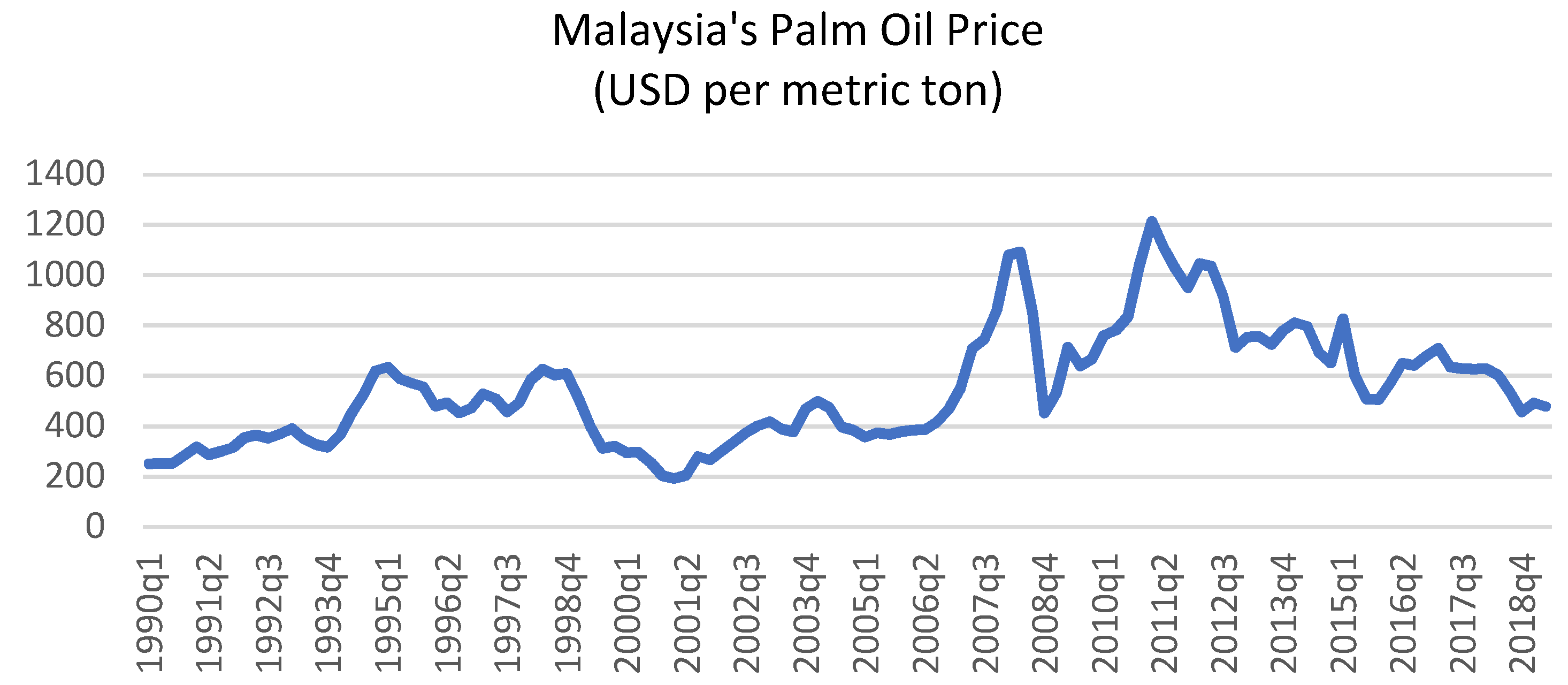
Figure 1 shows the movement of the Malaysia’s palm oil price from 1990 to 2019. There are several sharp ups and downs. As can be seen, the price began to increase significantly beginning quarter 2, 2006 and had a significant peak at quarter 1, 2008 (USD1092 per metric ton). The price dropped significantly after that until it reached to previous level of 2016 (USD452 per metric ton) at quarter 4, 2008. This was the results of the global financial crisis originating from subprime crisis in the US. Most countries have been affected, and it has led to a decrease in the demand for palm oil. 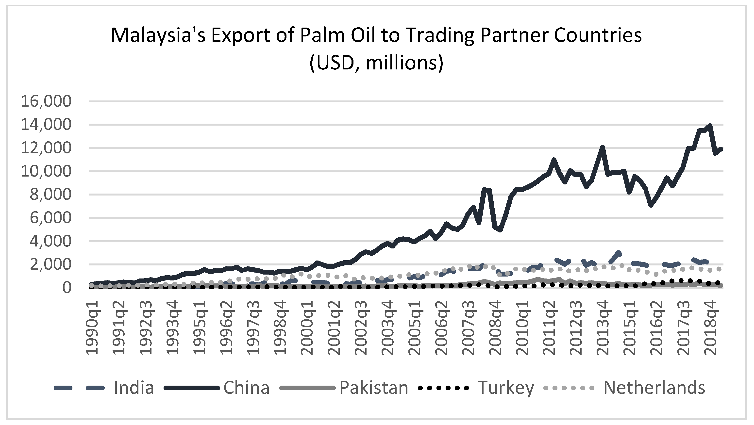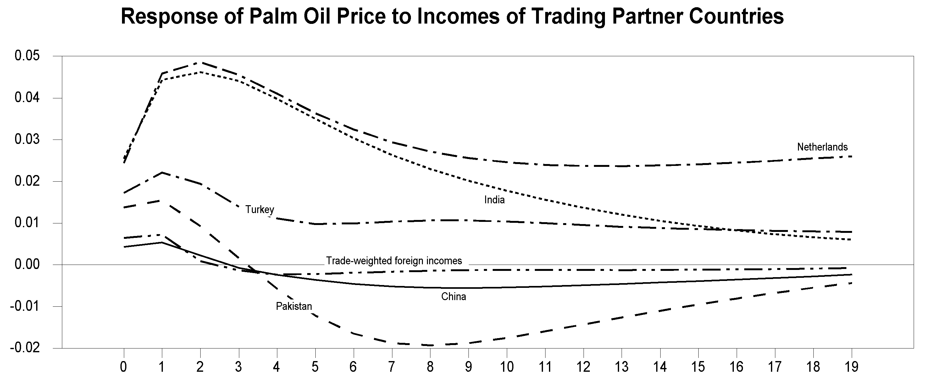Figure 2 shows that the exports of Malaysia’s palm oil to its top five trading partner countries in palm oil; namely, China, India, Pakistan, Turkey, and the Netherlands dropped significantly during the global financial crisis. Since quarter 4, 2008, the palm oil price started to have a positive trend until it reached the highest peak in quarter 1, 2011 (USD1213 per metric ton). The price then had several ups and downs in downward trending.

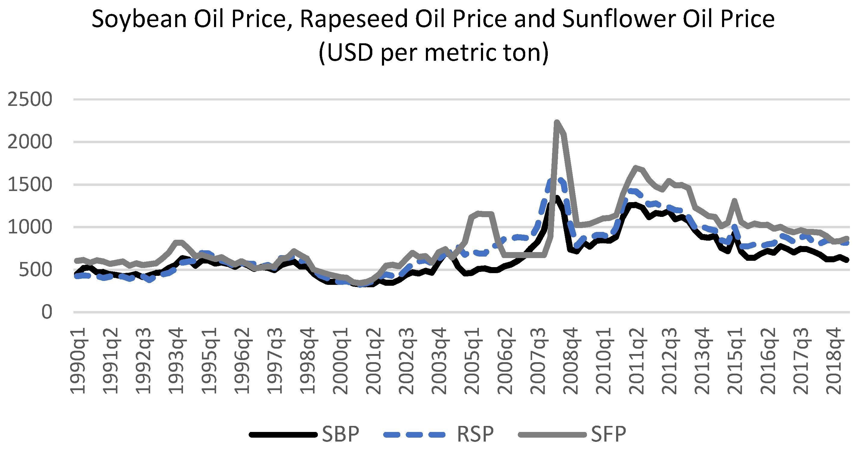
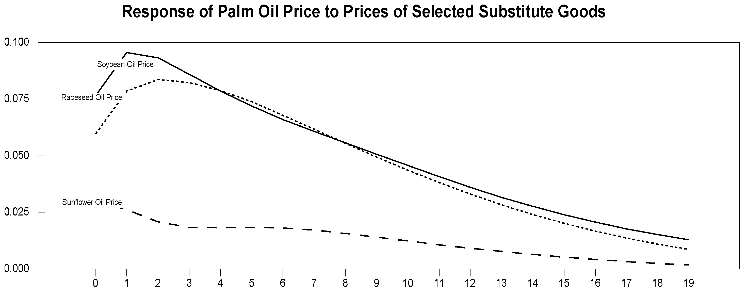
Figure 3 depicts the prices of substitution goods to palm oil, namely soybean oil, rapeseed oil, and sunflower oil. The trends of those prices resemble the ups and downs of the price of palm oil and this is an indication of how stiff the competition is among the oils and fats commodities.

Factors affecting the palm oil price can come from external and internal sources representing the demand as well as the supply factors. The external factors comprise the prices of palm oil’s substitution goods such as soybean oil, rapeseed oil, and sunflower oil (Ismail et al. 2019; Wong and Ahmad 2017; Mahalik et al. 2014; Sehgal et al. 2013; Abdullah 2013), foreign importers’ income (Zakaria and Nambiappan 2019; Wong and Ahmad 2017), the world palm oil price, and the crude oil price (Abdullah 2011; Nazlioglu and Soytas 2012; Khalid et al. 2018; Buyung et al. 2017). Meanwhile, the internal factors include the production of the palm oil, income of the nation (Zakaria and Nambiappan 2019; Zakaria et al. 2017; Kochaphum et al. 2013), and the palm oil export.

The fluctuation of palm oil raises concerns for those who deal with the risks and uncertainties in the palm oil industry and may affect smallholder income, thereby affecting the country’s revenues in the future. Therefore, understanding the main factors that affect palm oil price movement is crucial to this industry’s stakeholders, particularly for small-farmers, plantation firms, and businesses to plan their business and activities in this industry.

Previous studies on palm oil price focus on identifying its determinants where the relationship between palm oil price with its substitution goods price, especially the soybean oil price, is often being emphasized (Chuangchid et al. 2012; Mohammadi et al. 2015; Hassan and Nambiappan 2016). Other studies look at the aspects of forecasting (Khalid et al. (2018), Abdul Hamid and Shabri (2017), Arasim and Karia (2015) and Karia et al. (2013)) and volatility of the palm oil price (Mahalik et al. 2014; Ab Rahman et al. 2007).

One area that is missing in the previous studies is understanding the relative effect of external and internal shocks on the movement of the palm oil price. Most previous studies usually consider several factors that can have an impact on the price of palm oil. Those factors can be categorized as foreign and domestic factors. Understanding the relative importance of foreign and domestic factors on the movement of the palm oil price would be beneficial to governments and various stakeholders in strategizing actions for mitigating risks associated with the fluctuation of the palm oil price. Thus, realizing the gap, this paper examines relative importance of external and internal shocks on the movement of palm oil price in Malaysia.

The paper fills the literature gaps in the following ways. First, this study considers more relevant economic shocks (foreign and domestic) to understand further how the exogenous shocks affect the crude palm oil price movement. In total, there are four external shocks and four domestic shocks that would be investigated in the model. Second, this study improves the previous studies by Khalid et al. (2018), Kochaphum et al. (2013), Ab Rahman et al. (2013) and Abdullah (2011) which did not consider the elements of structural shocks in their model, by analyzing the propagation of the exogenous shocks through impulse response function (IRF) and forecast error variance decomposition (FEVD) on the movement of the palm oil price. Third, this study investigates the relative effects of palm oil’ substitution goods, namely soybean oil, rapeseed oil, and sunflower oil, on the Malaysia’s palm oil price. Results of IRF and VD would indicate which substitution goods play a more dominant role in affecting the palm oil price. Fourth, the study examines how the shocks to foreign incomes of Malaysian major trading partners in the palm oil market, namely India, China, Pakistan, Turkey, and Netherlands influence the palm oil price movement. Besides measuring foreign income using the trade-weighted of India, China, Pakistan, Turkey, and Netherlands’s incomes, following the approach of Zaidi et al. (2013), this study also considers each trading partner country’s income to represent the foreign income measure, respectively. Various considerations in the modeling process might also serve as robustness checks.

This study contributes to the stakeholders of the palm oil industry and to the literature in the following ways. First, to the stakeholders, this study may encourage the policymakers to understand main factors that influence the palm oil price, so that they can react accordingly to lessen uncertainty of income for the small farmers and businesses, as well as to plan for stabilizing the palm oil price. Understanding the palm oil price movement’s main factors is also crucial for the government to plan its strategic trade policy and implement a new strategy to diversify in the international market. It is vital for farmers and businesses to understand the main factors affecting the movement of the palm oil price because their future income depends on those factors; consequently, they can strategize to mitigate the adverse effect of the shocks on their income.

Second, to the literature, this study extends the existing literatures (Khalid et al. 2018; Abdul Hamid and Shabri 2017; Arasim and Karia 2015; Ab Rahman et al. 2013) that have focused on forecasting and volatility of the palm oil price and the factor that affects the movement of palm oil price in the Malaysia’s context. The previous studies in the Malaysian context, nonetheless, have ignored how the propagation of an internal and external shock affects palm oil price movement. Thus, this study takes advantage of the SVAR methodology to examine these issues where the structural shocks’ identification is based on the economic theory. Furthermore, the study implements block exogeneity restrictions in the SVAR specification to portray the real situation where the block of domestic variables from small open economy (Malaysia) would not affect, neither contemporaneously nor with lags, on the block of foreign variables. An exception is on the domestic production of the palm oil that is assumed to affect the world palm oil price since Malaysia is among the top producers of the palm oil.

The remainder of this paper is organized as follows. Section 2 describes the data and research design. Section 3 discusses the empirical results of the impulse response function and variance decomposition that have been estimated using the SVAR approach, and Section 4 concludes.

2. Data and Methodology

2.1. Data and Description of Variables

This study utilizes quarterly frequency data from 1990 to 2019. The period included several crises that may contribute to shocks in the palm oil price. Variables that have shown connections with the palm oil price as stated in the past literatures were considered for this study. Thus, the variables under investigation were crude oil price, prices of the palm oil substitution goods such as soybean oil, sunflower oil, and rapeseed oil, foreign income from Malaysia’s major trading partners in palm oil (India, China, Pakistan, Turkey, and Netherlands), world and Malaysia palm oil prices, Malaysia’s production of CPO, Malaysia’s palm oil export, Malaysia’s Gross Domestic Product, and real exchange rate. The details about the variables are summarized in

Table 1. Description of variables.

Variable	Notation	Description
Crude Oil Price	CRO	Crude Oil Price in US dollar (USD) per barrel
Foreign Income	YF	Trade-weighted of Top 5 Malaysia’s Trading Partner in Palm Oil *
India’s Income	GDPI	India’s Gross Domestic Product (USD)
China’s Income	GDPC	China’s Gross Domestic Product (USD)
Pakistan’s Income	GDPP	Pakistan’s Gross Domestic Product (USD)
Turkey’s Income	GDPT	Turkey’s Gross Domestic Product (USD)
The Netherlands’ Income	GDPN	The Netherlands’ Gross Domestic Product (USD)
Soybean Oil Price	SBP	Soybean Oil Price in US dollar (USD) per metric ton
Rapeseed Oil Price	RSP	Rapeseed Oil Price in US dollar (USD) per metric ton
Sunflower Oil Price	SFP	Sunflower Oil Price in US dollar (USD) per metric ton
World Palm Oil Price	CPOW	World Palm Oil Price in US dollar (USD) per metric ton
Crude Palm Oil Production	YCPO	Crude Palm Oil Production in a thousand ton (‘000)
Crude Palm Oil Price	CPOM	Malaysia Crude Palm Oil Price in US dollar (USD) per metric ton
Crude Palm Oil Export	CPOX	Crude Palm Oil Export in a thousand ton (‘000)
Domestic Income	GDPM	Malaysia Gross Domestic Product (USD)
Real Exchange Rate	REER	Malaysia Real Exchange rate

* The trade weightage is based on export of Malaysia to the five most important trading partner in palm oil.

.

All the data were gathered from Malaysia Palm Oil Board (MPOB), International Financial Statistic (IFS), International Monetary Fund (IMF), and Thomson Reuters. All variables are transformed into logarithm form.

2.2. Empirical Models

This study adapted structural vector autoregressive (SVAR) procedures employed by Amisano and Giannini (1997) and Khan and Ahmed (2014). The SVAR is used to capture exogenous economic shocks on Malaysia’s palm oil price. The approach is useful to test the interdependent relationship between the variables under consideration. Moreover, the model enables us to determine the structural shocks based on economic theory and it gives relevant empirical results than other VAR classes.

There are in total 8 SVAR models to be estimated. Each model has nine variables.

Table 2. Variables used in each SVAR model.

Variables	Model 1	Model 2	Model 3	Model 4	Model 5	Model 6	Model 7	Model 8
1	CRO	CRO	CRO	CRO	CRO	CRO	CRO	CRO
2	YF	YF	YF	GDPI	GDPC	GDPP	GDPT	GDPN
3	SBP	RSP	SFP	SBP	SBP	SBP	SBP	SBP
4	CPOW	CPOW	CPOW	CPOW	CPOW	CPOW	CPOW	CPOW
5	YCPO	YCPO	YCPO	YCPO	YCPO	YCPO	YCPO	YCPO
6	CPOM	CPOM	CPOM	CPOM	CPOM	CPOM	CPOM	CPOM
7	CPOX	CPOX	CPOX	CPOX	CPOX	CPOX	CPOX	CPOX
8	GDPM	GDPM	GDPM	GDPM	GDPM	GDPM	GDPM	GDPM
9	REER	REER	REER	REER	REER	REER	REER	REER

shows the variables used in each model. Model 1 is the main model where the impulse response functions are generated and discussed in detail. The first model, following the approach of Zaidi et al. (2013), considers trade-weighted income variables of Malaysia’s top five trading partners, namely India, China, Pakistan, Turkey, and the Netherlands, to represent the foreign income. The price of substitute goods of soybean oil (SBP) is considered since soybean oil is the perfect substitute good for palm oil as they have similarities in function. Model 2 and model 3 have the same variables as in model 1 except the substitute goods to palm oil are different. Model 2 utilizes RSP, while model 3 uses SFP. Models 4 to 8 have individual partner countries’ GDP to represent the foreign income respectively. Comparing the IRF and FEVD of models 1 to 3 would indicate the relative importance of substitution goods to explain the variation in the palm oil price shock. Similarly, comparing the IRF and FEVD of models 4 to 8 would uncover the relative importance of the partners’ countries income to reveal the variation in the palm oil price shock.

As with other VAR models, an optimal lag length is determined to remove serial correlation in the residuals. The selection of the lag length is based on the Akaike Information Criterion (AIC) and Schwarz Bayesian Criterion (SBC). To test the stationarity of the time series, unit root tests of augmented Dickey–Fuller (ADF) and Phillip–Perron (PP) were performed on each variable. One of the concerns when using time series data is the occurrence of spurious regression when non-stationary time series are used in the regression model. With regard to that, there are considerable discussions about whether to estimate the structural VAR in levels, first-differenced, or in a cointegration-imposed VAR. Some past literatures tend to suggest estimating a structural VAR in level even if the times series have unit roots (Sims et al. 1990; Christiano et al. 1996; Ramaswamy and Sloek 1997; Ashley and Verbrugge 2009; Basher et al. 2012). According to Sims et al. (1990), the estimated coefficients of a VAR are consistent, and the asymptotic distribution of individual estimated parameters is standard when variables are not stationary and the cointegration relationship might exists in some of the variables. Since the primary aim of SVAR is to determine interdependence among the variables, it may not be crucial to use differenced variables, although the unit root might exist (Sims 1980; Sims et al. 1990). Moreover, differentiating variables can exclude signals related to the co-movement of data (Enders 2004).

This study would primarily use impulse response function and forecast error variance decomposition to examine the interrelationship between the time series. The impulse response functions from the VAR model are consistent estimators of their true impulse response functions for the short and medium run only (Basher et al. 2012). Phillips (1998) shows that, in the long run, the standard impulse responses do not converge to their true values and are thus not consistent in the unrestricted VARs with some unit roots. To address this issue, this study also considers alternative impulse responses based on local linear projections as suggested by Jorda (2005) as the approach is robust to the problem. This study would mainly discuss the impulse response functions for the short run and the medium run.

Following Amisano and Giannini (1997) and Khan and Ahmed (2014), the SVAR is written as:

$$A{Y}_t=C+\left({\mathsf{\Gamma }}_{1}L+{\mathsf{\Gamma }}_1{L}^2+\dots \dots +{\mathsf{\Gamma }}_k{L}^k\right)Y_t+{\epsilon }_t.$$

(1)

The equation shows the dynamic relationships for the selected economic variables in the SVAR approach where A is a square matrix that captures the structural contemporaneous relationships among the economic variables. $Y_t$ represents n-vector of relevant variables as follows:

$$Y_t=\left(CR{O}_t , Y{F}_t ,SB{P}_t ,CPO{W}_t ,YCP{O}_t ,CPO{M}_t , CPO{X}_t ,GDP{M}_t ,REE{R}_t\right){}^{\prime }$$

C is a vector of deterministic variables while Γ(L) represents a kth-order matrix polynomial in lag operator L. The structural shocks are denoted by ${\epsilon }_t=\left({\epsilon }_t^{lcro}, {\epsilon }_t^{lyf},{\epsilon }_t^{lsbp},{\epsilon }_t^{lcpow},{\epsilon }_t^{lycpo},{\epsilon }_t^{lcpom},{\epsilon }_t^{lcpox}, {\epsilon }_t^{lgdpm},{\epsilon }_t^{lreer}\right){}^{\prime }$.

The SVAR model cannot be estimated directly because it correlates with the other endogenous variables in one equation. Therefore, by pre-multiplying Equation (1) with $A^{-1}$, it will produce a reduced form VAR equation:

$$Y_t=A^{-1}C+A^{-1}\left({\mathsf{\Gamma }}_{1}L+{\mathsf{\Gamma }}_1{L}^2+\dots \dots +{\mathsf{\Gamma }}_k{L}^k\right)Y_t+A^{-1}{\epsilon }_t$$

(2)

where $e_t=A^{-1}{\epsilon }_t$ shows the reduced form VAR residual. It satisfies the $E\left(e_t\right)=0$, $E\left(e_t{e^{\prime }}_s\right)={{\displaystyle \sum }}_e.$ ${{\displaystyle \sum }}_e$ is a positive and definite $\left(n\times n\right)$ symmetric matrix which can be estimated efficiently. The residuals are also presumed to be white noise, but they may be correlated with each other because of the variables’ contemporaneous effect across the equation. The variance-covariance matrix of the estimated residuals, ${{\displaystyle \sum }}_e$ and the variance-covariance matrix of the structural innovations, ${{\displaystyle \sum }}_{\epsilon }$ is related as follows:

$${{\displaystyle \sum }}_{\epsilon }=E\left({\epsilon }_t{\epsilon }_t^{\prime }\right)=E(A{e}_t{e}_t^{\prime }{A}^{\prime })=AE\left(e_t{e}_t^{\prime }\right)A^{\prime }=A{{\displaystyle \sum }}_e{A}^{\prime }$$

(3)

Sufficient restrictions must be imposed for the system to be identified to recover all the parameters in the structural equations. For $\left(n\times n\right)$ symmetric matrix of ${{\displaystyle \sum }}_e$, the unknowns are $(n^2+n)$/2. Thus, additional restrictions of $(n^2+n)$/2 must be imposed to exactly identify the system.

2.3. The Structural Model

Structural innovations ${\epsilon }_t$ and the reduced-form residuals et are related by $A{e}_t={\epsilon }_t$. The elements above the matrix’s diagonal in A are all set equal to zero in a purely recursive SVAR model.

The set of restrictions that are imposed on the contemporaneous parameters of the SVAR model of the Malaysia palm oil price is indicated by Equation (4). The coefficient $a_{ij}$shows the contemporaneous effect of variable j on variable i. The diagonal coefficients are normalized to unity and there are 44 zero restrictions on the coefficients to make the model over-identified.

$$A{Y}_t=\left[\begin{array}{ccccccccc}1& 0& 0& 0& 0& 0& 0& 0& 0\\ {\alpha }_{21}& 1& 0& 0& 0& 0& 0& 0& 0\\ {\alpha }_{31}& {\alpha }_{32}& 1& 0& 0& 0& 0& 0& 0\\ {\alpha }_{41}& {\alpha }_{42}& {\alpha }_{43}& 1& {\alpha }_{45}& 0& 0& 0& 0\\ 0& 0& 0& 0& 1& 0& 0& 0& 0\\ {\alpha }_{61}& {\alpha }_{62}& {\alpha }_{63}& {\alpha }_{64}& {\alpha }_{65}& 1& 0& 0& 0\\ 0& {\alpha }_{72}& {\alpha }_{73}& {\alpha }_{74}& {\alpha }_{75}& 0& 1& 0& 0\\ {\alpha }_{81}& {\alpha }_{82}& 0& {\alpha }_{84}& 0& 0& {\alpha }_{87}& 1& 0\\ {\alpha }_{91}& {\alpha }_{92}& {\alpha }_{93}& {\alpha }_{94}& {\alpha }_{95}& {\alpha }_{96}& {\alpha }_{97}& {\alpha }_{98}& 1\end{array}\right]\left[\begin{array}{c}{CRO}_t\\ {YF}_t\\ {SBP}_t\\ {CPOW}_t\\ {YCPO}_t\\ {CPOM}_t\\ {CPOX}_t\\ {GDPM}_t\\ {REER}_t\end{array}\right]$$

(4)

The construction of the structural identification is based on empirical findings of previous literature and economic theory. There are two blocks of variables, namely the foreign block and the domestic block. The variables in the foreign block are the price of crude oil, foreign income, world palm oil price, and the price of palm oil’s substitute goods such as soybean oil prices. Meanwhile, palm oil production, palm oil price, palm oil export, domestic income, and real exchange rate represent variables in the domestic block. The crude oil price is assumed to be exogenous and does not react to any demand and supply shocks because it is the one which affects demand and supply factors. Foreign variables are generally exogenous to domestic variables, which means the domestic variables are assumed not to contemporaneously affect the foreign variables since the Malaysian economy is relatively small and, therefore, unlikely to impact foreign variables. An exception is on Malaysia’s palm oil production. Since Malaysia is among the largest producers of the palm oil, Malaysian palm oil production is assumed to affect the world palm oil price contemporaneously as well as with lags. The palm oil price however reacts immediately to shocks to all foreign variables and the production of palm oil itself. Export of palm oil price is assumed to respond contemporaneously to foreign income, palm oil substitute goods (i.e., soybean oil price), world palm oil price, and the palm oil production shocks. In the meantime, the domestic income reacts immediately to shocks to crude oil price, foreign income, world palm oil price and palm oil export. Lastly, since real exchange rate is a fast-moving variable, it responds contemporaneously to all variables’ shocks. It would only affect other variables above it with lags as demand and supply factors could not be materialized immediately.

The IRF is carried out to track each variable’s current and future responses due to the change or shock of a particular variable and the variable’s time to the shock until the effect disappears or returns to its original state. A bootstrapping technique is used to generate one standard error confidence bands for the impulse response where a total of 2500 random samples (with replacement) are drawn from the original sample data. FEVD is also conducted to track the transmission channel to determine which shock has had a major role in explaining each variable in the model. FEVD predicts the percentage contribution of each variable due to changes in certain variables in the VAR system. This analysis will help determine relative importance of internal and external shocks in affecting the crude palm oil price in Malaysia.

3. Empirical Results and Discussion

This section first briefly explains the optimum lag of the chosen model which is model 1, before analyzing the propagation of the internal and external shocks on the movement of palm oil price. The optimum lag length has been identified using Akaike’s information criterion (AIC) and Schwarz Bayesian criterion (SBC). As reported in

Table 3. Results of lag length test.

Number of Lags	AIC	SBC
0	−11.13	−10.92
1	−27.72	−25.71 *
2	−27.81 *	−24.31
3	−26.65	−22.05
4	−25.10	−19.92

* indicates optimal lag length.

, SBC criteria selects one lag while AIC criteria selects two lags as optimum. The study employs two lags in order to have dynamics in the system. For stability tests, all the eigenvalues from the selected model are less than one; therefore, the estimation model of SVAR is stable.

3.1. Results of Stationarity Tests

Table 4. Results of the unit root tests.

Augmented Dickey–Fuller				Phillips–Perron
Level Form		1st Difference		Level Form		1st Difference
CRO	−1.5948 [1]	DCRO	−8.5776 [0] ***	CRO	−1.2484 [4]	DCRO	−8.5970 [4] ***
YF	0.0199 [3]	DYF	−5.7478 [2] ***	YF	0.0881 [4]	DYF	−10.2202 [4] ***
GDPI	0.5012 [1]	DGDPI	−7.6977 [0] ***	GDPI	0.4675 [4]	DGDPI	−7.8293 [4] ***
GDPC	−0.2859 [0]	DGDPC	−4.3002 [4] ***	GDPC	−0.2923 [4]	DGDPC	−10.3379 [4] ***
GDPP	−0.3419 [4]	DGDPP	−3.2483 [4] **	GDPP	−0.2228 [4]	DGDPP	−3.6825 [4] ***
GDPT	−0.9232 [4]	DGDPT	−4.5443 [4] ***	GDPT	−1.1745 [4]	DGDPT	−8.1201 [4] ***
GDPN	−0.9965 [4]	DGDPN	−6.4458 [3] ***	GDPN	−1.3940 [4]	DGDPN	−7.9228 [4] ***
SBP	−1.9093 [1]	DSBP	−8.6148 [0] ***	SBP	−1.8341 [4]	DSBP	−8.5915 [4] ***
RSP	−1.8597 [1]	DRSP	−8.1809 [0] ***	RSP	−1.7086 [4]	DRSP	−8.1982 [4] ***
SFP	−2.4756 [1]	DSFP	−7.2524 [2] ***	SFP	−2.0251 [4]	DSFP	−7.7241 [4] ***
CPOW	−2.5248 [1]	DCPOW	−7.7252 [0] ***	CPOW	−2.3451 [4]	DCPOW	−7.6616 [4] ***
YCPO	−1.8013 [4]	DYCPO	−10.0225 [3] ***	YCPO	−1.0115 [4]	DYCPO	−14.0748 [4] ***
CPOM	−2.6196 [1] *	DCPOM	−7.6484 [0] ***	CPOM	−2.4187 [4]	DCPOM	−7.5765 [4] ***
CPOX	−1.7274 [4]	DCPOX	−7.9244 [4] ***	CPOX	−0.9613 [4]	DCPOX	−17.1749 [4] ***
GDPM	−1.3760 [4]	DGDPM	−5.6023 [4] ***	GDPM	−1.2720 [4]	DGDPM	−5.9665 [4] ***
REER	−2.0245 [0]	DREER	−12.5555 [0] ***	REER	−1.8947 [4]	DREER	−12.7707 [4] ***

Notes: Figures in parenthesis are the optimal lag based on AIC. *, ** and *** denote statistical significant at the 10%, 5% and 1% levels, respectively.

shows results of the unit root tests on each time series. Based on the augmented Dickey–Fuller (ADF) and Phillips–Perron (PP) tests, all the time series were stationary at first difference or I(1). Further tests of stationarity with structural break on the time series, as shown in

Table 5. Results of unit root test with structural break.

Minimize Dickey Fuller
Level Form		Break Date	1st Difference		Break Date
CRO	−3.8227 [1]	2003:3	DCRO	−8.9497 [0] ***	1991:1
YF	−2.5938 [4]	2001:4	DYF	−10.4014 [0] ***	1991:3
GDPI	−2.6001 [8]	2003:1	DGDPI	−9.8200 [0] ***	1991:3
GDPC	−2.8657 [4]	2004:3	DGDPC	−14.4766 [0] ***	1994:1
GDPP	−2.1527 [12]	2003:1	DGDPP	−3.8439 [0]	1992:1
GDPT	−5.1577 [4] ***	2002:3	DGDPT	−8.2369 [0] ***	1993:2
GDPN	−4.2763 [4] *	2002:1	DGDPN	−8.8629 [0] ***	2008:4
SBP	−3.0427 [10]	2006:3	DSBP	−8.6394 [0] ***	1993:3
RSP	−3.6425 [1]	2002:2	DRSP	−9.1371 [0] ***	2008:4
SFP	−4.4217 [1] *	2004:2	DSFP	−7.8786 [0] ***	1993:3
CPOW	−3.9223 [1]	2006:2	DCPOW	−9.1731 [0] ***	2008:4
YCPO	−4.8783 [12] **	1999:1	DYCPO	−11.8639 [0] ***	1993:2
CPOM	−3.9653 [1]	2006:2	DCPOM	−9.0800 [0] ***	2008:4
CPOX	−3.9139 [5]	1999:1	DCPOX	−14.0710 [0] ***	1991:1
GDPM	−2.7975 [3]	2003:3	DGDPM	−6.6120 [0] ***	2008:4
REER	−5.0674 [0] ***	1997:2	DREER	−13.9084 [0] ***	1997:4

Notes: Figures in parenthesis are the optimal lag based on AIC. GDPP appears to be I(2) after further investigation. *, ** and *** denote statistical significant at the 10%, 5% and 1% levels, respectively.

, indicate that almost all the time series were I(1) except for GDPT, GDPP, SFP, YCPO, and REER which were I(0). GDPP appeared to be I(2). Nevertheless, all variables used in the selected model (model 1) were either I(0) and I(1). As mentioned, the study proceeded to use the impulse response function and variance decomposition from the SVAR model. According to Ramaswamy and Sloek (1997), there was a tradeoff between the loss of efficiency when the VAR was estimated in levels, without enforcing any cointegrating relationships, and the loss of information when the VAR was regressed in first differences. They suggest not to impose cointegration restrictions on the VAR model in cases where there is no prior economic theory that can imply either the number of long-run relationships, or how they should be explained. A similar approach has been undertaken by Basher et al. (2012). This paper thus specifies the SVAR model in levels.

3.2. Impulse Response Function

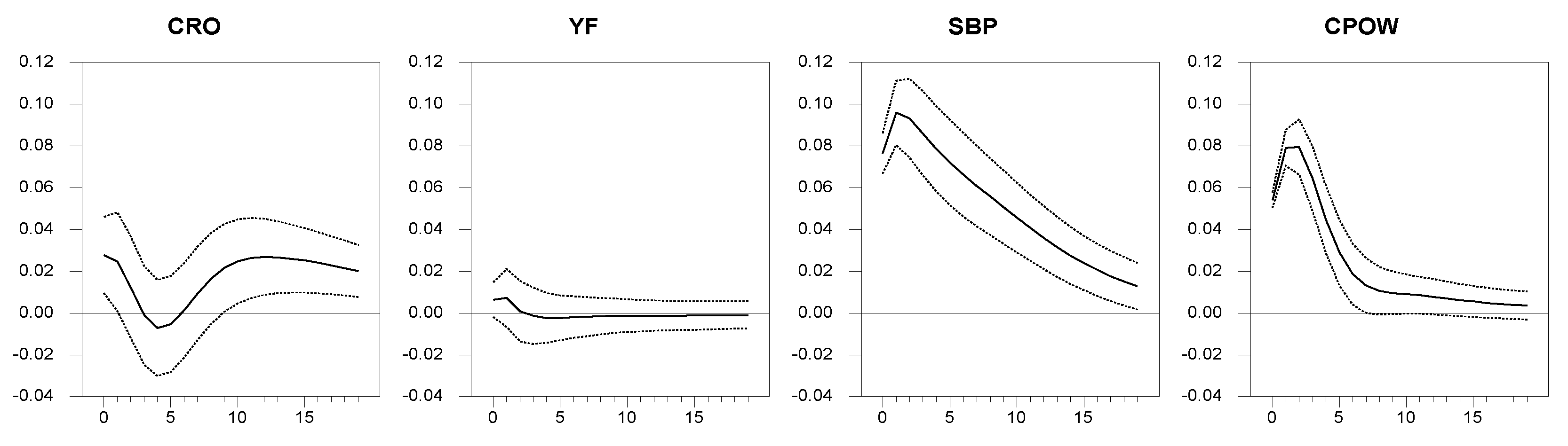
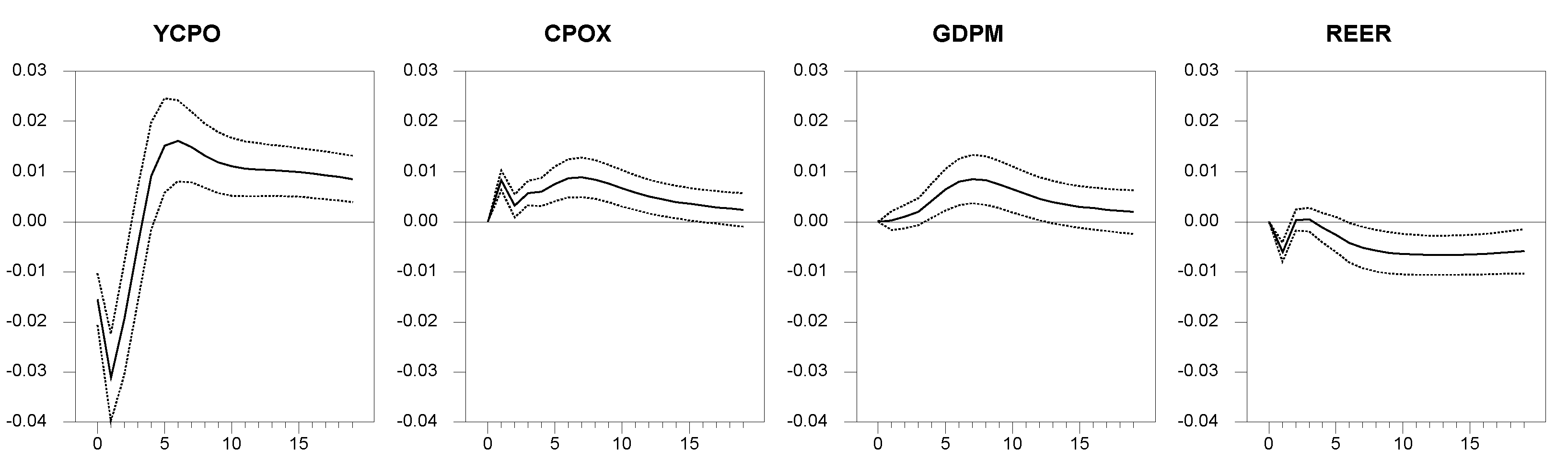
Figure 4 and Figure 5 show the responses of palm oil price to external and internal shocks respectively. The external shocks are represented by shocks to the world crude oil price, the foreign income, the soybean oil price, and the world palm oil price. On the other hand, internal shocks are represented by Malaysia’s palm oil production, Malaysia’s palm oil export, Malaysia’s domestic income, and the exchange rate. In explaining the impulse response functions, the study only emphasizes the short run and the medium run impact. 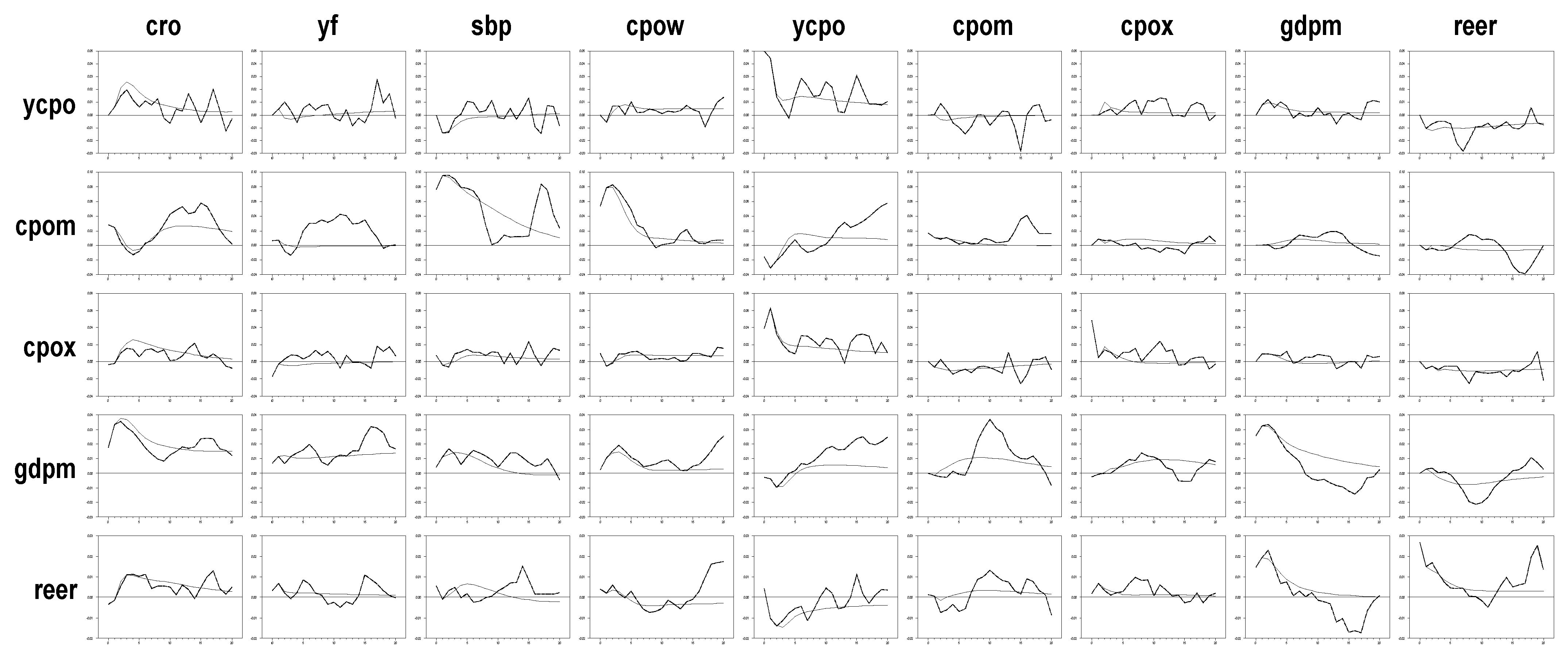Appendix A show the impulse response functions from the SVAR estimation as well as the impulse response functions based on local projections as suggested by Jorda (2005). It can be seen that the impulse responses from local projections in the long run are quite different from that of the impulse responses from the SVAR.

From Figure 4, a shock to the world crude oil price significantly affects the palm oil price movement in Malaysia. The palm oil price initially shows a positive and significant response in the first quarter before subsiding in the second quarter. It responds positively and significantly again after the eight quarters. This indicates the importance of the crude oil price in influencing Malaysia’s palm oil price movement. According to Buyung et al. (2017), the crude oil price impacts the demand and supply of the commodity price.

Meanwhile, a shock to the foreign income (trade weighted income from 5 major palm oil importers) does not give significant impact on the palm oil price even though the palm oil price responds positively to the foreign income shock. Investigating the impact of each trading country’s shock on the palm oil price movement might give some indications about the importance of a particular foreign country on the palm oil price. This is discussed later in this section.

On the other hand, a shock to the soybean oil price significantly affects the palm oil price movement. The highest magnitude of the palm oil price response is in the first quarter before subsiding gradually. This indicates that the soybean oil price has an immediate large effect on the palm oil price movement. Theoretically, an increase in the price of soybean oil leads to an increase in the demand for palm oil and in turn has a positive impact on the palm oil price. This finding is supported by most of the past literature (Ismail et al. 2019; Zakaria et al. 2017; and Hassan and Nambiappan 2016) which reveals that the palm oil substitute goods is the main factor that affects the movement of palm oil price.

Similarly, the world palm oil price also plays a vital role in affecting the palm oil price movement. A shock to the world palm oil price significantly and positively impacts the Malaysia’s palm oil price for most of the quarters under study. This finding indicates that the Malaysia’s palm oil price also responds to the movement of the world palm oil price, although Malaysia is one of the largest producers and exporters of the palm oil in the world market.

Figure 5 shows the responses of the palm oil price to the internal shocks. As depicted, the most significant domestic variables that impact the palm oil price movement is the production of the palm oil itself. A shock to the production of palm oil has a negative and significant impact on the palm oil price movement for about four quarters. This might be due to the excess supply of the palm oil in the short run. However, the palm oil price responds positively and significantly beginning the fifth quarter.

Responses of the palm oil price to the palm oil export and to the domestic income shocks are mainly positive. The positive magnitude of the responses to both shocks are about the same. Palm oil export portrays the demand for palm oil in the market; therefore, theoretically, an increase in the demand for the palm oil leads to an increase in the palm oil price. Wong and Ahmad (2017), however, uncovered a negative relationship between palm oil and export. As Malaysia is one of the largest countries to export the palm oil, this study indicated that a shock in the palm oil export affects the palm oil price positively. Similarly, a shock to the domestic income would lead to an increase in the demand for the palm oil thru an increase in consumption. This in turn affects the palm oil price positively. In line with Zakaria and Nambiappan (2019), domestic income brings a positive effect to palm oil demand.

Meanwhile, a shock to the exchange rate has significantly led to a decrease in the palm oil price in the first two quarters. In other words, an appreciation in Ringgit Malaysia has led to a decrease in the palm oil price. This is in line with Ismail et al. (2019) study where the exchange rate has short term negative effect on the palm oil price.

Figure 6 depicts the responses of the palm oil price to a shock to the rapeseed oil price as well as to a shock to the sunflower oil price. Apparently, the effect of soybean oil price shock is bigger than the other two shocks in the short run. This further proves that soybean oil price is important in describing the movement in the palm oil price. Similar findings are reported in Ismail et al. (2019), Zakaria et al. (2017) and Hassan and Nambiappan (2016).

Responses of the palm oil price to a shock in the foreign income from the major Malaysian trading partners in palm oil, namely India, China, Pakistan, Turkey, and the Netherlands, on the movement of palm oil price are summarized in Figure 7. As can be seen, a shock to India’s income and a shock to the Netherlands’ income bring about the same significant positive short run effects on the movement of the palm oil price. The effect of Turkey’s income comes next, and it is followed by Pakistan’s income and China’s income, respectively. Thus, using individual country’s income indicates better responses of the palm oil price to a foreign income shock. Consequently, the study contributes to reveal the importance of investigating the effect of individual trading partner countries on the palm oil price movement.

Model 1 in

Table 6. Variance decompositions for the palm oil price from various measurement of substitute goods prices.

Decomposition of Variance for Series CPOM—Model 1
Step	Std Error	CRO	YF	SBP	CPOW	YCPO	CPOM	CPOX	GDPM	REER
1	0.1005	7.676	0.417	57.862	28.953	2.374	2.717	0	0	0
5	0.2512	2.522	0.163	59.026	34.28	2.666	1.015	0.232	0.036	0.06
10	0.2939	2.841	0.136	65.046	26.885	3.135	0.832	0.564	0.374	0.187
15	0.3130	6.015	0.127	64.308	24.013	3.324	0.736	0.639	0.45	0.388
20	0.3211	8.251	0.126	62.768	22.919	3.573	0.7	0.649	0.457	0.558
Decomposition of Variance for Series CPOM—Model 2
Step	Std Error	CRO	YF	RSP	CPOW	YCPO	CPOM	CPOX	GDPM	REER
1	0.1033	6.213	0.707	33.325	50.704	6.331	2.72	0	0	0
5	0.2584	2.098	0.488	44.553	41.22	10.36	0.925	0.184	0.003	0.168
10	0.3011	3.082	0.662	54.239	32.268	8.246	0.841	0.251	0.087	0.324
15	0.3175	6.308	0.883	54.555	29.223	7.452	0.796	0.271	0.131	0.382
20	0.3259	9.051	1.137	52.804	28.346	7.078	0.772	0.272	0.142	0.398
Decomposition of Variance for Series CPOM—Model 3
Step	Std Error	CRO	YF	SFP	CPOW	YCPO	CPOM	CPOX	GDPM	REER
1	0.1026	6.933	0.349	8.66	75.269	6.113	2.677	0	0	0
5	0.2613	2.651	0.12	3.965	80.337	11.343	1.234	0.221	0.015	0.114
10	0.2972	4.67	0.105	4.668	79.116	9.402	1.162	0.485	0.247	0.146
15	0.3122	8.755	0.096	4.698	75.753	8.577	1.066	0.55	0.368	0.136
20	0.3190	11.508	0.094	4.565	73.486	8.23	1.022	0.555	0.383	0.156

summarizes the results of FEVD for propagating external and internal shocks on the movement of palm oil price. As can be seen, foreign shocks explain most of the variation in palm oil price movement. For example, within 20 quarters, foreign shocks contributed about 94.1% (the sum of the proportions of forecast error variance of palm oil price explained by CRO, YF, SBP, and CPOW) compared with domestic shocks that only contributed 5.9%. These findings imply that external factors play a dominant role than internal factors in influencing Malaysia’s palm oil price movement. The most critical foreign factor is the soybean oil price, which has contributed about 57.9% of the palm oil price variation even at the first quarter. Model 2 and model 3 reveal variance decomposition of the palm oil price when other substitute goods of the palm oil, namely rapeseed oil price and sunflower oil price are in place, respectively. Comparing those three models indicates that the soybean oil price has contributed the biggest proportion than the other substitution goods’ prices in explaining the variation in the palm oil price.

Table 7. Variance decompositions for the palm oil price from various measurement of foreign incomes.

Decomposition of Variance for Series CPOM—Model 1
Step	Std Error	CRO	YF	SBP	CPOW	YCPO	CPOM	CPOX	GDPM	REER
1	0.1005	7.676	0.417	57.862	28.953	2.374	2.717	0	0	0
5	0.2512	2.522	0.163	59.026	34.28	2.666	1.015	0.232	0.036	0.06
10	0.2939	2.841	0.136	65.046	26.885	3.135	0.832	0.564	0.374	0.187
15	0.3130	6.015	0.127	64.308	24.013	3.324	0.736	0.639	0.45	0.388
20	0.3211	8.251	0.126	62.768	22.919	3.573	0.7	0.649	0.457	0.558
Decomposition of Variance for Series CPOM—Model 4
Step	Std Error	CRO	GDPC	SBP	CPOW	YCPO	CPOM	CPOX	GDPM	REER
1	0.1003	7.74	0.189	56.627	30.271	2.475	2.697	0	0	0
5	0.2500	2.551	0.095	56.139	36.565	2.729	1.41	0.359	0.056	0.097
10	0.2918	3.127	0.213	61.484	29.019	3.109	1.316	0.899	0.527	0.306
15	0.3107	6.648	0.311	60.347	25.82	3.276	1.234	1.098	0.686	0.579
20	0.3186	9.042	0.345	58.653	24.594	3.455	1.217	1.185	0.732	0.776
Decomposition of Variance for Series CPOM—Model 5
Step	Std Error	CRO	GDPI	SBP	CPOW	YCPO	CPOM	CPOX	GDPM	REER
1	0.1004	7.894	6.445	49.99	30.463	2.694	2.514	0	0	0
5	0.2530	2.829	12.947	44.82	35.117	3.3	0.766	0.166	0.009	0.046
10	0.2949	4.031	13.875	50.553	27.864	2.636	0.591	0.271	0.103	0.075
15	0.3145	8.576	13.215	49.938	24.723	2.445	0.521	0.281	0.131	0.169
20	0.3231	11.597	12.799	48.517	23.475	2.434	0.495	0.282	0.142	0.259
Decomposition of Variance for Series CPOM—Model 6
Step	Std Error	CRO	GDPP	SBP	CPOW	YCPO	CPOM	CPOX	GDPM	REER
1	0.1010	7.785	1.85	54.482	31.607	2.102	2.175	0	0	0
5	0.2490	2.865	0.887	55.495	37.524	2.317	0.673	0.166	0.026	0.048
10	0.2888	3.921	2.45	59.758	30.398	2.442	0.528	0.32	0.082	0.101
15	0.3111	9.171	3.191	57.167	27.036	2.367	0.468	0.335	0.087	0.179
20	0.3238	13.413	3.183	54.573	25.359	2.35	0.469	0.312	0.11	0.231
Decomposition of Variance for Series CPOM—Model 7
Step	Std Error	CRO	GDPT	SBP	CPOW	YCPO	CPOM	CPOX	GDPM	REER
1	0.1007	7.074	2.944	56.025	28.302	2.871	2.784	0	0	0
5	0.2508	2.497	2.362	58.521	32.361	3.065	0.799	0.248	0.089	0.06
10	0.2898	2.418	2.4	65.767	25.343	2.789	0.612	0.326	0.255	0.089
15	0.3035	4.19	2.689	65.839	23.214	2.706	0.565	0.317	0.252	0.228
20	0.3085	5.691	2.955	64.616	22.52	2.728	0.55	0.311	0.259	0.371
Decomposition of Variance for Series CPOM—Model 8
Step	Std Error	CRO	GDPN	SBP	CPOW	YCPO	CPOM	CPOX	GDPM	REER
1	0.0993	7.037	6.067	51.238	29.787	3.053	2.818	0	0	0
5	0.2495	2.274	14.181	45.506	32.136	4.51	0.994	0.269	0.065	0.064
10	0.2881	2.686	16.216	50.423	25.477	3.394	0.82	0.464	0.415	0.107
15	0.3041	5.029	17.659	49.566	22.888	3.051	0.739	0.483	0.485	0.101
20	0.3126	6.186	19.924	47.506	21.744	2.898	0.701	0.469	0.477	0.096

compares FEVD for the palm oil price from model 1, and model 4 through model 8. Various foreign income variables were used to see the effect of each foreign income as well as the aggregate one in explaining the variation in the palm oil price. Assessing those models reveals that India’s income as well the Netherlands’ have more profound effects on the palm oil price as compared to income shocks from the other trading partners. As shown, at the end of five quarters, India’s income explains about 12.8% while the Netherlands’ income explains about 19.9% of the variation in the palm oil price. In the meantime, the trade-weighted foreign income only explains 0.1% of the variation in the palm oil. Thus, the study indicates that employing individual foreign income in the model would give clearer picture of the impact of a particular foreign country’s income on the palm oil price.

3.3. Robustness Test

As mentioned, several alternative substitution goods prices and foreign income variables are used in the SVAR model to see their impacts on the palm oil price. This has served for sensitivity analysis or robustness test to the selected model (model 1). The study has also reordered CRO and FY, where FY is placed at the top in the identification scheme shown in Equation (4), indicating that foreign output to have contemporaneous effect on the crude oil price. In addition, the study has also assumed that CRO and FY might influence each other. In other words, in the identification structure, CRO could have contemporaneous effect on the foreign income and foreign income could have an impact on the CRO from the perspective of the demand side. This would made α₁₂ to be non-zero in the identification matrix [4].

Interestingly, the results of IRF to changes in the alternative variables as well as in alternative identification approaches do not differ significantly from the IRF of the chosen model especially with respect to impulses responses of Malaysia’s palm oil to external and internal factors. Consequently, this shows that the SVAR model is robust to alternative selection of variables as well as of identification structures.

4. Conclusions

This paper examines the relative importance of foreign shocks (crude oil price, foreign income, substitute good of palm oil, and world palm oil price) and domestic shocks (palm oil production, palm oil export, domestic income, and real effective exchange rate) on the movement of Malaysia’s palm oil price. A non-recursive SVAR identification scheme has been used to examine the propagation of the exogenous shocks (foreign and domestic shocks) to the palm oil price using IRF and FEVD approaches. Specifically, IRF indicates the effect of external and internal factors’ shocks on the movement of the palm oil price while the FEVD show which factors explain the most of the variation in the palm oil shock.

The main findings reveal that foreign factors play a crucial role in influencing Malaysia’s palm oil price. In particular, the palm oil’s substitute goods’ price, such as soybean oil price, plays a dominant role in explaining the palm oil price movement. These findings are aligned with the standard demand theory and the previous literatures which state that an increase in the price of the palm oil substitute goods would increase palm oil demand and in turn increase the palm oil price. Furthermore, foreign income shocks from major trading partners, namely India and the Netherlands, are also important in influencing the movement of Malaysia’s palm oil price. Shocks to internal factors are also important in affecting the movement of the palm oil price. Nevertheless, the magnitudes of the effects are rather small as compared to the external factors’ shocks.

The findings of the study have several implications for the stakeholders in the palm oil industry. First, since the external shocks play a crucial role in influencing the palm oil price, the small farmers and the palm oil-oriented firms need to take precautions to the changes in the external factors in managing and strategizing their palm oil production activities. This is because any shocks to the external factors would influence the palm oil price and in turn affect the small farmers’ future income and the palm oil-oriented firms’ profit. Thus, to mitigate the adverse income flow consequences of the external factor shocks, the small farmers and the palm oil-oriented firms need to plan alternative use of their palm oil production, for example, making it as intermediate goods for other palm oil related products.

Second, the policymakers in the palm oil sector, particularly the Malaysian Palm Oil Board (MPOB) and Ministry of Plantation Industries and Commodities can take advantage of the findings to further understand the magnitude and the signs of the external and internal shocks that affect the palm oil price. This is important for the policymakers to assist affected smallholders’ groups during adverse shocks of the external factors that directly affect the palm oil sector’s performance. Proper dissemination of knowledge about the adverse effects of external and internal factors to smallholders might help them strategically plan for alternative activities.

Third, since foreign incomes, mainly from India and the Netherlands, affect the palm oil price quite substantially, Malaysia exporters need to diversify and find new market to avoid high dependency on the traditional markets. Diversifying export of the palm oil into new markets can reduce income uncertainty from a conventional market. For example, Malaysia could aggressively market the palm oil to other MENA countries (other than Turkey) which have shown increasing interest in the palm oil products. Finally, taking into consideration the related external factors, policy makers can strategically control domestic palm oil output in order to maintain the palm oil price.

Nevertheless, the study has some limitations. First, the study did not go through pre-testing of cointegration. Following the approaches of Ramaswamy and Sloek (1997), and Basher et al. (2012), the study proceeded to use the SVAR model. The primary concerned was not at the coefficients of the estimation themselves, but rather the interrelationship among the variables through the IRF and FEVD analysis. Interestingly, the SVAR model was structured with block exogeneity restriction, according to real situation, where the domestic variables do not affect the external variables either contemporaneously or with lags since Malaysia is a small open economy. An exception is on the LYCPO where the Malaysia’s production of palm oil is assumed to have an impact on the world palm oil since Malaysia is the second largest palm oil producer. Second, as mentioned the validity for the impulse response functions from the SVAR estimation are for the short run and the medium run only. For the long run, the impulse response functions should be referred to local projection suggested by Jorda (2005). This is showed in Appendix A. For future research, researchers might want to investigate in details how various substitution goods’ prices such as soybean oil price, rapeseed oil price and sunflower oil price affect volatility of the palm oil price. Similarly, researchers can also look at the volatility of the palm oil price that might be caused by various trading partner countries’ income.