Abstract
The performance of a free-space optical (FSO) communications link suffers from the deleterious effects of weather conditions and atmospheric turbulence. In order to better estimate the reliability and availability of an FSO link, a suitable distribution needs to be employed. The accuracy of this model depends strongly on the atmospheric turbulence strength which causes the scintillation effect. To this end, a variety of probability density functions were utilized to model the optical channel according to the strength of the refractive index structure parameter. Although many theoretical models have shown satisfactory performance, in reality they can significantly differ. This work employs an information theoretic method, namely the so-called Jensen–Shannon divergence, a symmetrization of the Kullback–Leibler divergence, to measure the similarity between different probability distributions. In doing so, a large experimental dataset of received signal strength measurements from a real FSO link is utilized. Additionally, the Pearson family of continuous probability distributions is also employed to determine the best fit according to the mean, standard deviation, skewness and kurtosis of the modeled data.
1. Introduction
The technology of free-space optical (FSO) communications, after decades of research efforts, seems to be ready to bring a revolution to the area of telecommunications. Yet, a few final burdens need to be overcome. This new technology promises to meet the requirements for increased data rates transmission for many current applications and also support the fiber-optic backbone networks by solving the last-mile problem [1]. The major obstacle in deploying an FSO link is the various effects of the laser beam traveling along the atmosphere. Atmospheric extinction, due to aerosols and molecules that cause the light beam to be absorbed or scattered, often leads to intensity degradation even to such a degree that can permanently interrupt the link. Atmospheric turbulence is another phenomenon that seriously degrades the quality of an FSO link by causing intensity fluctuations to the receiver, beam wandering, angle-of-arrival fluctuations and beam spreading [1].
Therefore, the state of the weather conditions severely affects the reliability and availability of the link. In order to better estimate those performance metrics, an accurate model should be selected, according to the weather conditions and especially the atmospheric turbulence. Traditionally, a large number of probability density functions (PDFs) have been utilized to model the received optical power of an FSO link. The most widely used and accepted PDF models include the Log-Normal (LN), Gamma–Gamma (GG), Gamma, Weibull, K, I-K, Malaga, the Fisher–Snedecor F and the negative exponential [1,2,3]. In order to evaluate the performance of an optical communication system, various link parameters can be employed, such as the probability of detection, the outage probability, the average capacity and the outage capacity [1,4]. In any case, knowledge of the PDF of the received optical power is required; however, it is rather difficult to determine which PDF better fits the statistics of the received power data [1].
In the open technical literature, several PDF models are available for weak, moderate and strong turbulence. For example, the Log-Normal and the Gamma–Gamma distributions accurately describe the weak and moderate regime whereas the Gamma–Gamma, the negative exponential and the K-distribution yield a better fit for the strong regime [4]. Apart from selecting a distribution corresponding to the correct turbulence strength regime, it is risky to assume that only a certain one accurately fits the experimental data. Instead, it is critical to investigate the best fit among different distributions.
In the past, extensive research work to estimate the performance of FSO links under various atmospheric conditions and communication schemes has been conducted. For example, Jose Maria Garrido et al. analyzed the performance of an FSO link affected by atmospheric turbulence and line-of-sight (LOS) blockages. They modeled the intensity fading due to turbulence using the Malaga distribution and derived a closed-form expression for the outage probability (OP). Their results showed a strong dependency of the LOS impact to the OP on the turbulence strength [5]. In [6], the scintillation effect has been modeled by the Gamma–Gamma and the I-K distribution to study the time dispersion and atmospheric turbulence in the performance of an FSO link and closed-form mathematical expressions for the evaluation of the link’s fade probability derived. Peppas et al. elaborated on the end-to-end capacity of dual hop FSO systems employing amplify-and-forward (AF) relaying. The link’s performance is affected by atmospheric turbulence, modeled by the Gamma–Gamma distribution, pointing errors and atmospheric absorption and derived analytical approximations for the channel’s ergodic capacity [7]. Wayne, in his dissertation [8], proposed a new physics-based technique to derive an analytical expression for the PDF of the irradiance, by taking into consideration the turbulence and aperture averaging effects and taking into account parameters directly related to measurable atmospheric parameters. The Log-Normal and Gamma–Gamma distributions have been utilized in [9] to derive closed-form expressions for the average capacity of an FSO link. An experimental work has been presented in [10] that provides a methodology for modeling laser beam’s intensity in a maritime environment and the corresponding PDF has been computed by using field measurements. Barrios, in his dissertation [11], proposed the exponentiated Weibull (EW) distribution for modeling the irradiance fluctuations in FSO links under atmospheric turbulence and taking into consideration the aperture averaging effect.
Motivated by the above, the main contribution of this paper is to propose a methodology of comparing different theoretical distribution models, for any turbulence strength regime. In doing so, a large experimentally measured dataset of received signal strength of an FSO link in the maritime environment is utilized and different theoretical PDF models are fitted to the entire dataset histogram. The Kullback–Leibler (KL) and Jensen–Shannon (JS) divergences are initially employed to compare five theoretical models and the best fit is determined by the absolute value of the corresponding divergence. Additionally, the Pearson family of probability distribution functions, consisting of seven types of continuous probability distributions, is utilized to determine the type that best fits to experimental data. The rest of the paper is organized as follows. Section 1 provides the theoretical background of the atmospheric turbulence and channel modeling. Section 2 describes the experimental setup and the data acquisition process. Section 3 provides the theoretical background of the KL and JS divergence, the Pearson distribution family and the model comparison results, whereas Section 4 concludes the paper.
1.1. Atmopsheric Turbulence
Atmosphere can be described as a fluid with two distinct motion states. One with uniform motion characteristics, the laminar, and another where uniformity disappears and random sub-flows occur, called turbulent eddies [12]. This motion state is a result of temperature and moisture gradients that cause changes in the refractive index of the atmosphere. This phenomenon, called optical turbulence, is highly non-linear and is described by the Navier–Stokes equations [13]. Turbulence theory, as it is known nowadays, is based on Kolmogorov approach based on dimensional analysis and approximations of Navier–Stokes equations. According to the Kolmogorov’s cascade energy theory, turbulence can be described by unstable air masses, called eddies, which by inertial energy transfer begin from the macroscale L0, i.e., outer scale and end at the microscale l0, i.e., inner scale. An important assumption of this theory is that eddies smaller than L0 are statistically homogeneous and isotropic [13]. Due to this characteristic, the covariance of the refractive index reduces to a function of solely a scalar distance R = |R1 − R2|2, where R1 and R2 are two random points in space. Then, the structure function within the inertial subrange, i.e., l0 << R << L0, is [13],
where Cn2 is the refractive index structure parameter. A point estimate of Cn2 can be easily obtained by measuring the temperature difference within two points with known separation distance. This can be done by using a set of thermocouples, with various numbers of fine wires. Another important parameter is the temperature structure parameter, CT2, which is related to Cn2 as follows [13],
where P and T the related pressure and temperature of that specific point. Path-averaged Cn2 measurements can also be taken using an instrument called scintillometer. A large number of experimental research works have led to the construction of many empirical models, for any kind of terrain, range and geometry of measurements, which can give good estimates for the refractive index structure parameter along the path, assuming constant values. A comprehensive list of Cn2 predictive models can be found in Tab. 2.5 [12].
1.2. Channel Modeling
In order to establish an FSO communications link with high reliability and availability, reasonable estimations of several statistical parameters related to the phenomenon of scintillation should be made. Signal fading can significantly degrade the link’s performance and increase the bit error rate (BER). Therefore, an accurate formulation of the PDF of these random fluctuations would allow a better prediction of the link’s reliability and thus it should be taken into consideration during system design. Apparently, there is no PDF that could sufficiently model all kind of turbulence conditions. It is important to notice the importance of the tails of a PDF model, since this region yields important information regarding the detection and fading probability. The moments of the irradiance fluctuations for a given PDF is given as [14],
where I is the received irradiance and p(I) the corresponding PDF. Higher-order coefficients also exist and provide a useful mean of model comparison, considering the PDF tail contribution for non-Gaussian distributions. For practical reasons, we are looking for controllable models that allow for accurate prediction of the channel’s performance. Apart from turbulence effects, a PDF distribution is also affected by the aperture averaging effect that tends to reduce the deleterious effects of scintillation. Therefore, whenever modeling an optical channel and estimating the received power, we need to clarify whether a point receiver or an aperture with certain dimensions is assumed [1]. Due to its relatively simple form, the LN distribution is the most widely used turbulence model. Moreover, this model is assumed valid for a weak turbulence regime in case of a point receiver and all turbulence regimes for aperture averaged measurements [1]. The PDF of the LN distribution is given by [4],
where σ2 is the log-irradiance, which depends on the aperture diameter, the wavelength and turbulence strength. On the other hand, the GG distribution is obtained as the product of two independent gamma modeled distributions, modelling small and large scale fluctuations. The great advantage of the GG distribution is that its two parameters, a and b, are directly related to Cn2. The PDF of the GG distribution is given as [4],
where Kq(.) is the modified Bessel function of the second kind of order q. The parameters a and b are directly related to turbulence and system parameters for a spherical wave as follows [4],
where the Rytov variance for a spherical wave and , where k is the optical wavenumber, L the link’s length and D the diameter of the aperture.
As mentioned above, an accurate distribution model is necessary to estimate the performance of an optical link. A critical metric related to system’s availability is the system’s outage probability, defined as the probability that the receiver’s signal-to-noise (SNR) ratio γ falls below a critical threshold γth [4]. Mathematically, this is expressed as,
where Fγ is the corresponding cumulative distribution function (CDF) of the SNR. The outage probability can now be expressed in accordance with the model that has been used to model the turbulent channel. Using the relation between irradiance, instantaneous and average SNR [4], i.e.,
the corresponding expression for the outage probability for the LN model is deduced as follows [4],
where erfc(.) denotes the complementary error function, whereas, for the GG model, Pout can be expressed as [4],
where G(.) is the Meijer’s G-function.
2. Data Acquisition
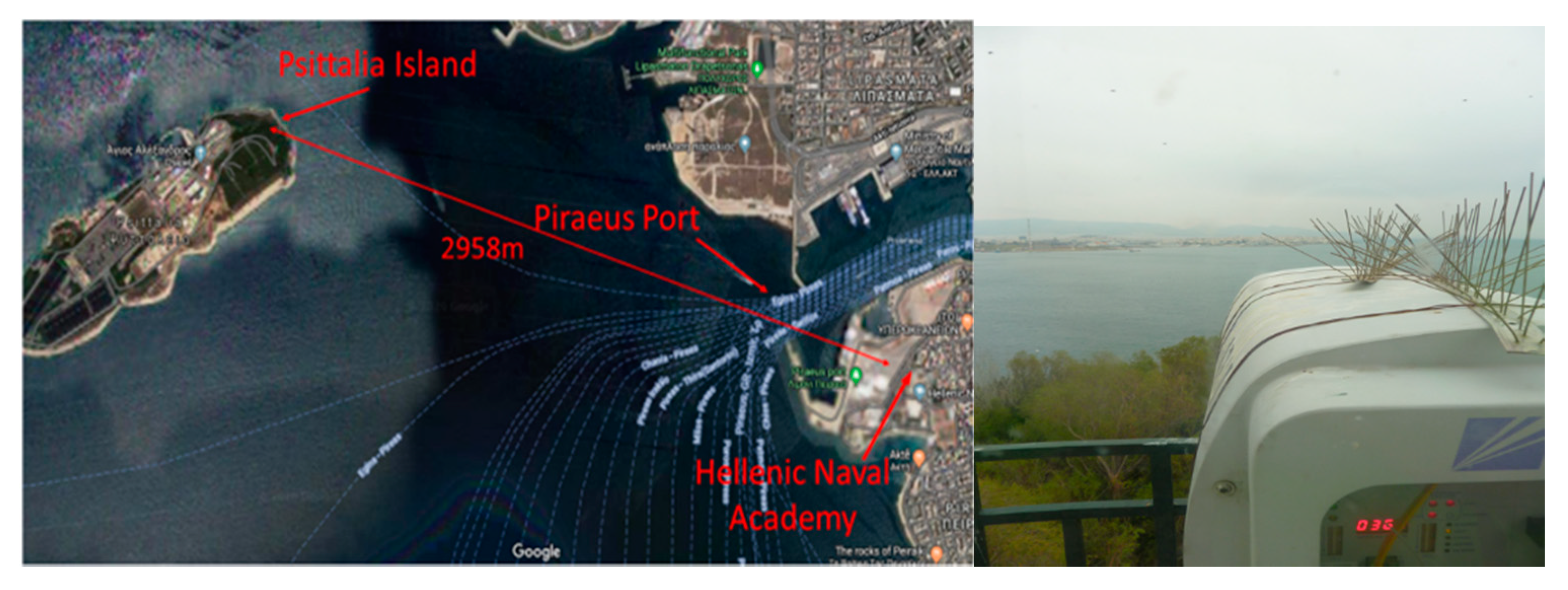
A commercial FSO communications system located on the Hellenic Naval Academy’s building roof and on Psitalia’s island lighthouse establishes an optical link with a length of 2958 m in a maritime environment [15]. The optical path has an average height above sea level of 35 m and almost 95% of it is above water. The operating FSO system is an MRV/TS5000/155, employing an Intensity Modulation/Direct Detection (IM/DD) communication scheme and yielding a maximum data rate of 155 Mbps (Figure 1). The selected metric for the FSO link performance evaluation was the received signal strength indicator (RSSI), a parameter that has been extensively used elsewhere [16,17,18,19]. The system has been set to obtain a measurement of the received signal strength indicator (RSSI) every minute, during each day, and then store these values in a connected PC for further analysis [20].

Figure 1.
The maritime free-space optical (FSO) link propagation path (left) and the MRV TS5000/155 FSO terminal on the lighthouse of Psitalia Island (right). On the upper left back side of the system, the received signal strength indicator (RSSI) indicator can be seen.
The data collection period of the RSSI parameter spanned over a year, from the 30 November 2019 to the 27 October 2020, to include 144,802 data points in total. At the same time, several macroscopic meteorological parameters were also measured from a standalone weather station located close to the FSO system so that their fluctuations can be monitored and estimate their influence on RSSI. This dataset of the RSSI measurements is used to apply the PDF fits comparison. The descriptive statistics of the dataset are shown in Table 1.

Table 1.
Descriptive statistics for the RSSI measurements from the 30 November 2019 to the 27 October 2020.
3. Results
In this section, we examine the fitting comparison techniques of different PDFs to an experimentally gathered dataset. This process will benefit the performance analysis of an FSO link and allow for credible reliability and availability estimations.
3.1. Kullback–Leibler Divergence
A fundamental information theoretical concept is the Kullback–Leibler (KL) divergence, providing a method to measure the conventionally defined “distance” among two distributions [21]. Let p and q be two distinct distributions defined on the same probability space, where p refers to a theoretical probability distribution and is measured against an experimental or modeled distribution, q. The KL divergence, also called the relative entropy, measures the inefficiency of assuming a distribution to be q when in reality it is p. The relative entropy or KL divergence between two distributions is given as [22],
The KL divergence is non-negative and asymmetric in p and q, i.e.,
The lower the value of the DKL, the less the distance between p and q, which ultimately becomes zero if the two distributions are identical. Additionally, if pi > 0 and qi = 0 for a given i, the KL divergence goes to infinity. Cover and Thomas give a technical interpretation of the KL divergence, as the “coding penalty” associated with a distribution q selected to compare with a distribution p [22].
Five theoretical distribution models where utilized to apply the Kullback–Leibler divergence Equation (11) in order to evaluate and compare their fit performance to the real-valued RSSI data. The theoretical PDFs used were:
The Kullback–Leibler divergence has been calculated for these five PDFs and the best fit to the observed RSSI data (30 November 2019–27 October 2020) was deduced. Initially, the frequency occurrence of each RSSI observation is calculated. The probability density of the RSSI data was then evaluated by dividing the frequency of each observation by the total number of observations. We then utilized the distfit MATLAB application to obtain the parameters of the theoretical distributions within the observed RSSI values range (187–517). By employing Equation (11) for each model, the KL divergence has been calculated (see Figure 2). The Burr distribution yields the best fit to experimental data and, as expected, it exhibited the lowest KL divergence value, 2.77 × 10⁻², followed by the Weibull distribution yielding a value of 3.07 × 10⁻².
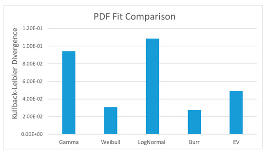
Figure 2.
The Kullback–Leibler divergence values for Gamma, Weibull, Lognormal, Burr and Extreme-Value distribution.
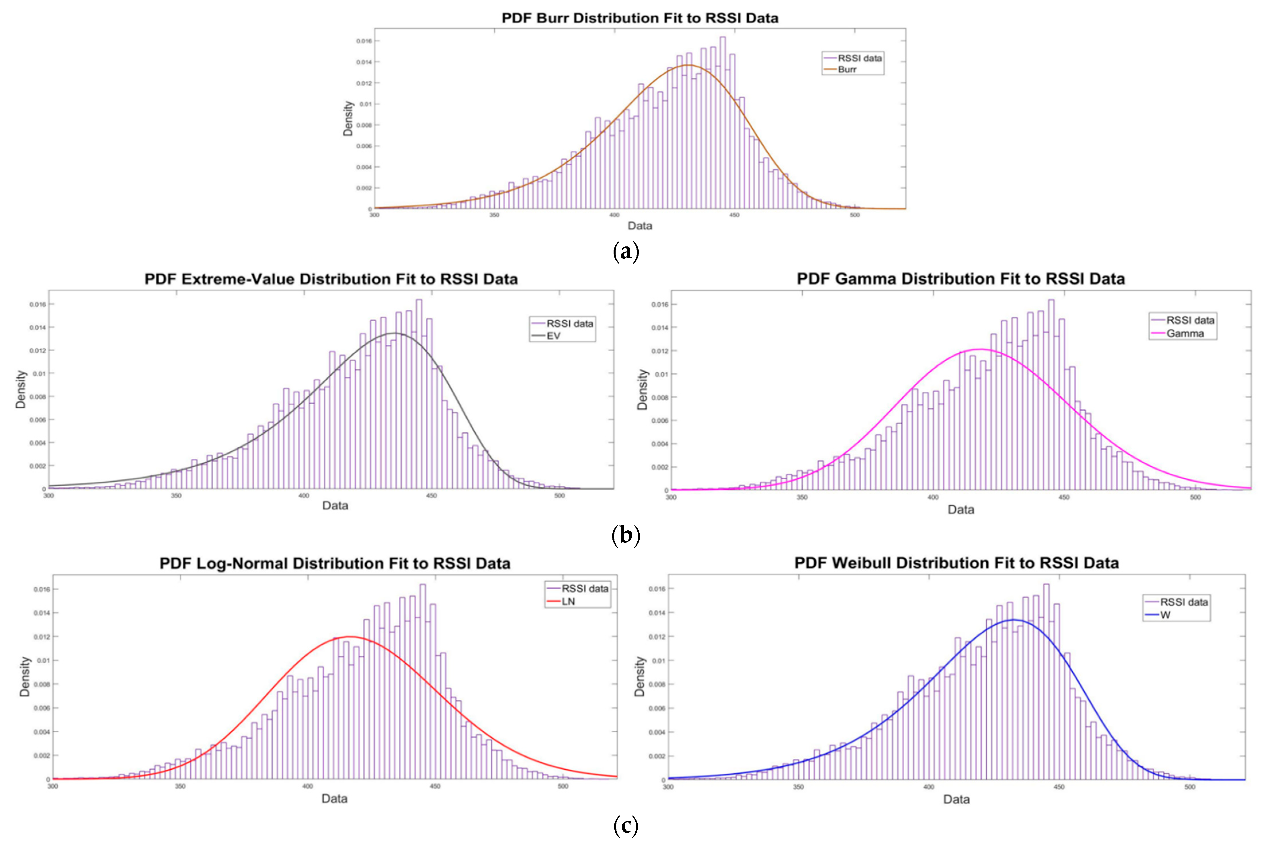
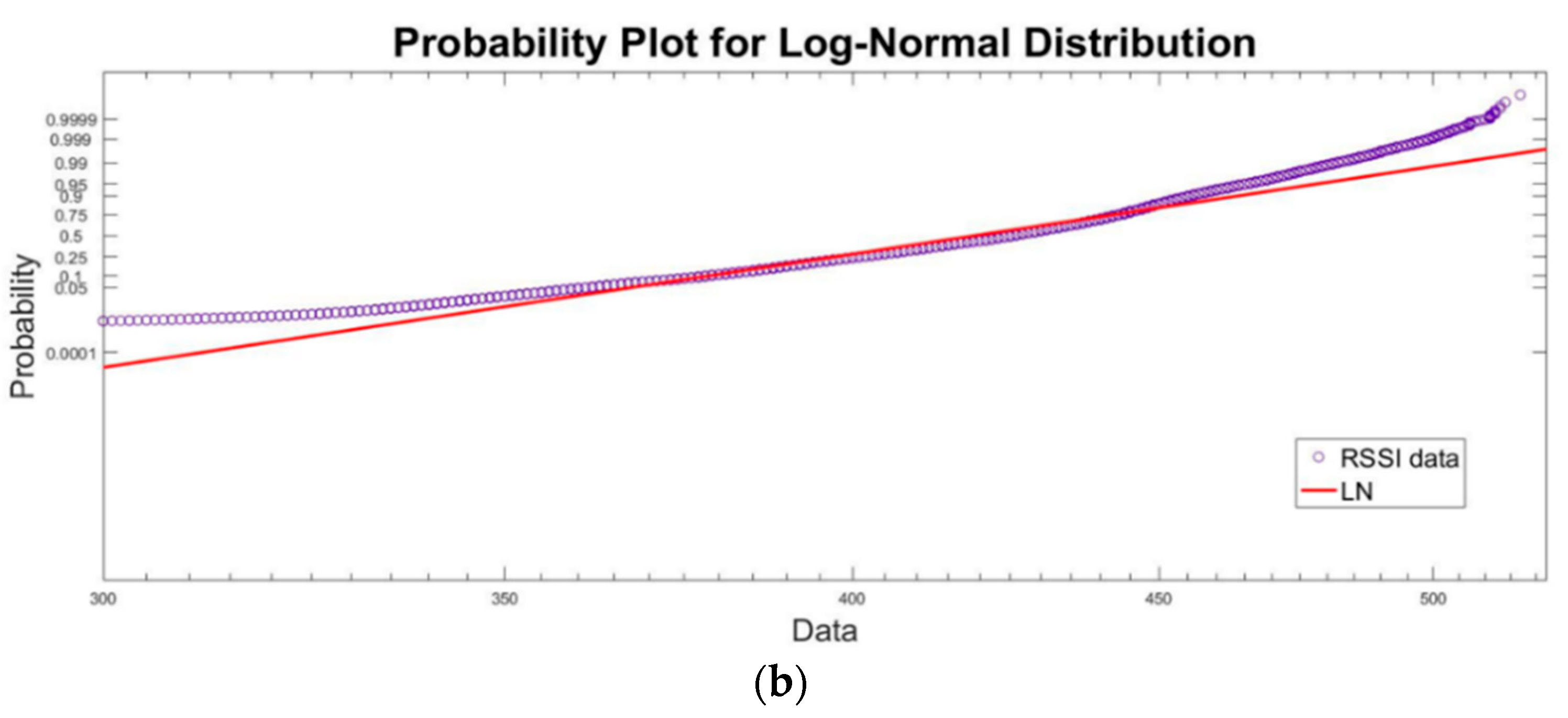
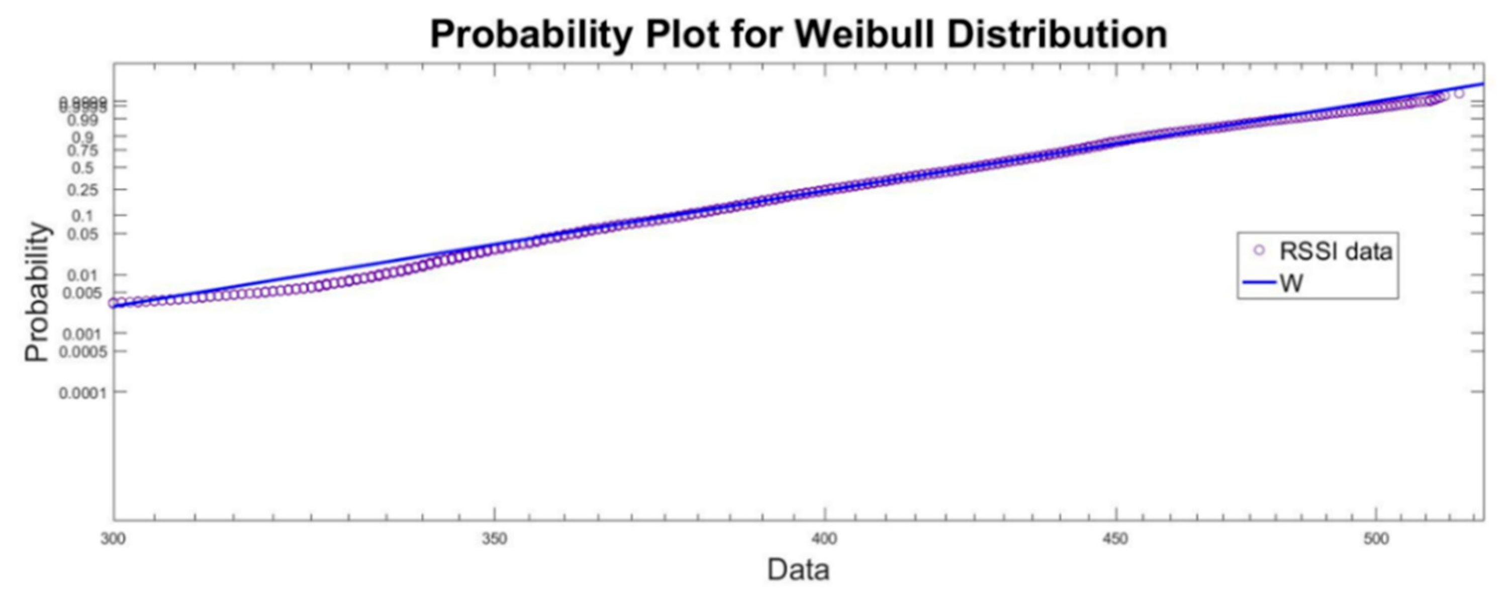
The PDFs for each theoretical model against the observed RSSI data are depicted in Figure 3, and their corresponding probability plots in Figure 4, Figure 5 and Figure 6.
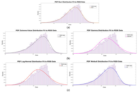
Figure 3.
Probability density functions fits to RSSI data for (a) Burr distribution, (b) Extreme-Value (left) and Gamma (right) distribution, (c) Log-Normal (left) and Weibull (right) distribution.
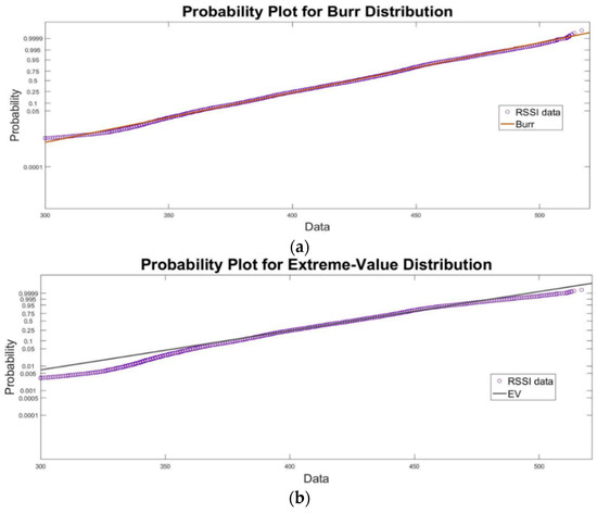
Figure 4.
Probability plots for (a) Burr and (b) Extreme-Value distribution against RSSI data.
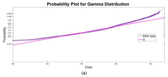
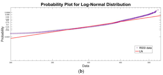
Figure 5.
Probability plots for (a) Gamma and (b) Log-Normal distribution against RSSI data.
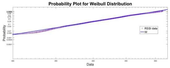
Figure 6.
Probability plot for Weibull distribution against RSSI data.
It is obvious graphically from the probability plots that the Burr distribution best fits the RSSI data. In particular, an excellent agreement with the experimental data is observed, with the exception of the far upper tail of the distribution. In contrast, the rest four of the tested distributions exhibit a noteworthy disagreement at both tails (Figure 4, Figure 5 and Figure 6).
3.2. Jensen–Shannon Divergence
Another method of measuring the similarity of two probability distributions is the so-called Jensen–Shannon divergence (JSD). The JSD is based on the KL divergence, however it exhibits a few but important differences with it, namely it is symmetric and it always has a finite value. The square root of JSD, also defined as the JS distance, is given by [23],
where M = (P + Q)/2, and D(P||M) and D(Q||M) are the KL divergences as defined by Equation (11). Provided that at least one of the two measured distributions uses base 2 logarithm, JSD is upper bounded by 1, namely
The JSD, also called the capacitory discrimination, can be interpreted as the total KL divergence to the average distribution, M [22]. Mathematically, it can also be defined as a Jensen divergence of the Shannon information h [22],
where the notation “;” is used instead, to emphasize its symmetry. Other symmetrizations of the KL divergence can be found in the literature, including the extrinsic Jensen–Shannon divergence, the Jeffreys divergence and the extended Kullback–Leibler divergence [24,25], among others. The JSD can also be defined as the mutual information between a random variable X and the binary indicator variable Z, used to switch between P and Q, whose mixture distribution is associated with X.
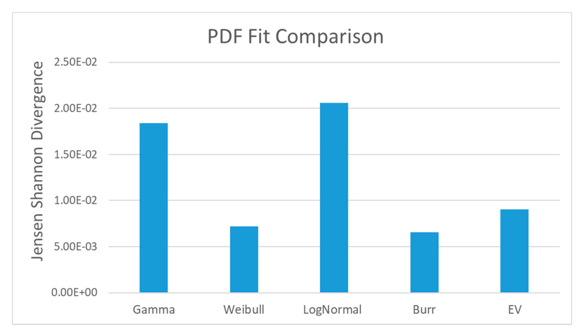
In order to calculate the JSD of each theoretical distribution against the observed RSSI data we employed Equation (14). The M parameter was deduced by taking the average between each model and the RSSI data, a total of five. Following that, we calculated the KL divergence between each distribution, including the RSSI data distribution, and the corresponding M parameter, which is a total of ten distinct KL values. Finally, the JSD is calculated and the results are shown in Figure 7.

Figure 7.
The Jensen–Shannon divergence values for Gamma, Weibull, Lognormal, Burr and Extreme-Value distribution.
3.3. Pearson Distribution Family
The Pearson family of continuous probability distributions has become popular within the research community due to its ability to take into account the skewness and kurtosis of a probability distribution. This fact is really valuable when theoretical probability distributions need to be fit to experimental data that exhibit skewness, which is the asymmetry of a real-valued data around their mean. Skewness can take negative, positive or zero values, where negative values indicate the distribution tails on the left, whereas positive values indicate distribution tails on the right. Pearson originally identified four types of distributions, characterized by two quantities, β1 and β2. Any valid solution of Equation (22) defines a Pearson type PDF [26].
where,
where λ is the location parameter of the distribution.
The solution for each type of Pearson distribution differs according to the values of parameters a, b, c and d. Many types included in Pearson family distributions are commonly used today in various applications, such as the beta, gamma and t-distribution [27].
The value of the discriminant of the quadratic function,
distinguishes the two main cases which group the distribution types.
We used the standard built-in function pearsrnd, available in MATLAB, in order to determine the type of Pearson distribution that best fits the observed RSSI data. The mean value, standard deviation, skewness and kurtosis of the RSSI data were used to calculate the parameters d, a, and b in Equation (24), where d = 0.0548, a = −0.3116 and b = 0.08355. Our experiments revealed that a Type IV Pearson PDF given by [27],
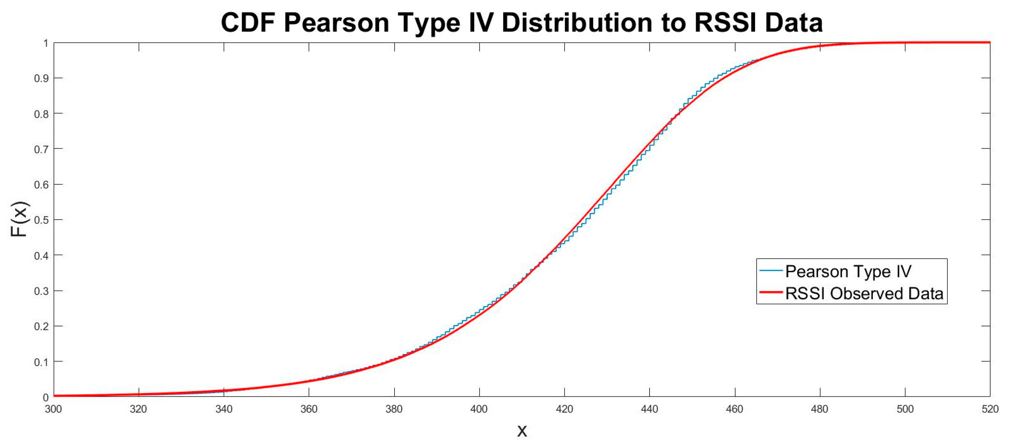
where A0 = b − c2(4d)−1 and A1 = c(2d)−1, yields the best fit. The Pearson Type IV cumulative distribution function (CDF) against the RSSI data is plotted in Figure 8 and a very good agreement is observed.
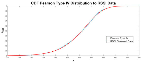
Figure 8.
The cumulative distribution function for Pearson Type IV against RSSI data.
4. Conclusions
In this work, the accuracy of five probability density functions to a large experimental dataset of the received signal strength for an FSO link was studied. The focus of this paper is to identify among those PDFs the one that best fits observed data, based on the available comparison methods. To this end, the Gamma, Lognormal, Extreme-Value, Burr and Weibull distributions were utilized to calculate initially their Kullback–Leibler divergence and a symmetrization of it, the Jensen–Shannon divergence, with the RSSI data. The Burr distribution was found to best fit the experimental data, with a KL and JS divergence values of 2.77 × 10⁻² and 6.53 × 10⁻³, respectively. The Weibull and EV distributions also exhibited a comparable accuracy in contrast with the Gamma and Lognormal, whose “distance” from real data was an order of magnitude higher. The Pearson distribution family of continuous probability functions was also used and experimental results showed that the type IV distribution yield the best fit. Both methods offer a straightforward process of comparing among different PDFs for accurately fitting real data. The two aforementioned methods follow a different approach to select the most appropriate PDF to fit to a dataset. The KL and JD metrics allow for the calculation of the performance metric of each candidate PDF, thus designating the best one as the one with the lowest divergence. From a practical point of view, the KL and JD metrics are more useful to apply in a real-world dataset, since they directly provide a certain output that allows any PDF to be examined. On the other hand, the selection of the best Pearson distribution using a moment matching method is preferable when a limited number of options for statistical modeling are available.
Author Contributions
Conceptualization, A.L., K.P.P., H.E.N.; methodology, A.L., K.P.P., H.E.N.; software, A.L.; validation, A.L., K.P.P., H.E.N. and A.T.; formal analysis, A.L., A.T.; investigation, A.L., K.P.P., H.E.N.; resources, A.L., K.P.P., A.T.; writing—original draft preparation, A.L., A.T.; writing—review and editing, A.L., K.P.P., H.E.N., A.T.; supervision, K.P.P., A.T., H.E.N. All authors have read and agreed to the published version of the manuscript.
Funding
This research received no external funding.
Institutional Review Board Statement
Not applicable.
Informed Consent Statement
Not applicable.
Conflicts of Interest
The authors declare no conflict of interest.
References
- Barrios, R.; Dios, F. Wireless Optical Communications through the Turbulent Atmosphere: A Review; Optical Communications Systems; Das, N., Ed.; InTech: Rijeka, Croatia, 2012; ISBN 978-953-51-0170-3. [Google Scholar]
- Jurado-Navas, A.; Garrido-Balsells, J.-M.; Paris, J.F.; Puerta-Notario, A. A Unifying Statistical Model for Atmospheric Optical Scintillation. In Numerical Simulations of Physical and Engineering Processes; Awrejcewicz, J., Ed.; InTech: Rijeka, Croatia, 2011; ISBN 978-953-307-620-1. [Google Scholar]
- Peppas, K.P.; Alexandropoulos, G.C.; Xenos, E.D.; Maras, A. The Fischer-Snedecor F-Distribution Model for Turbulence-Induced Fading in Free-Space Optical Systems. J. Lightwave Technol. 2019, 38, 1286–1295. [Google Scholar] [CrossRef]
- Nistazakis, H.E.; Katsis, A.; Tombras, G.S. On the Reliability and Performance of FSO and Hybrid FSO Communication Systems over Turbulent Channels; Nova Science Publishers, Inc.: Hauppauge, NY, USA, 2010; ISBN 978-1-61761-735-5. [Google Scholar]
- Garrido-Balsells, J.M.; Lopez-Martinez, F.J.; Castillo-Vázquez, M.; Jurado-Navas, A.; Puerta-Notario, A. Performance analysis of FSO communications under LOS blockage. Opt. Express 2017, 25, 25278–25294. [Google Scholar] [CrossRef] [PubMed]
- Varotsos, G.K.; Stassinakis, A.N.; Nistazakis, H.E.; Tsigopoulos, A.D.; Peppas, K.P.; Aidinis, C.J.; Tombras, G.S. Probability of fade estimation for FSO links with time dispersion and turbulence modeled with the gamma–gamma or the I-K distribution. Optik 2014, 125, 7191–7197. [Google Scholar] [CrossRef]
- Peppas, K.; Stassinakis, A.; Nistazakis, H.; Tombras, G. Capacity Analysis of Dual Amplify-and-Forward Relayed Free-Space Optical Communication Systems Over Turbulence Channels with Pointing Errors. J. Opt. Commun. Netw. 2013, 5, 1032–1042. [Google Scholar] [CrossRef]
- Wayne, D. The Pdf of Irradiance for A Free-Space Optical Communications Channel: A Physics Based Model. Ph.D. Thesis, University of Central Florida, Orlando, FL, USA, 2010. [Google Scholar]
- Nistazakis, H.E.; Karagianni, E.A.; Tsigopoulos, A.D.; Fafalios, M.E.; Tombras, G.S. Average Capacity of Optical Wireless Communication Systems Over Atmospheric Turbulence Channels. J. Lightwave Technol. 2009, 27, 974–979. [Google Scholar] [CrossRef]
- Korotkova, O.; Avramov-Zamurovic, S.; Malek-Madani, R.; Nelson, C. Probability density function of the intensity of a laser beam propagating in the maritime environment. Opt. Express 2011, 19, 20322–20331. [Google Scholar] [CrossRef] [PubMed]
- Ricardo, B. Exponentiated Weibull Fading Channel Model in Free-Space Optical Communications under Atmospheric Turbulence. Ph.D. Thesis, Polytechnic University of Catalonia, Barcelona, Spain, 2013. [Google Scholar]
- Kaushal, H.; Jain, V.K.; Kar, S. Free-Space Optical Channel Models; Springer: New Delhi, India, 2017. [Google Scholar] [CrossRef]
- Andrews, L.C.; Phillips, R.L.; Hopen, C.Y. Laser Beam Scintillation with Applications, 2nd ed.; SPIE: Bellingham, WA, USA, 2001. [Google Scholar]
- Majumdar, A.K. Free-space laser communication performance in the atmospheric channel. J. Opt. Fiber Commun. Rep. 2005, 2, 345–396. [Google Scholar] [CrossRef]
- Lionis, A.; Peppas, K.; Nistazakis, H.E.; Tsigopoulos, A.D.; Cohn, K. Experimental Performance Analysis of an Optical Communication Channel over Maritime Environment. Electronics 2020, 9, 1109. [Google Scholar] [CrossRef]
- Haluška, R.; Šuľaj, P.; Ovseník, Ľ.; Marchevský, S.; Papaj, J.; Doboš, Ľ. Prediction of Received Optical Power for Switching Hybrid FSO/RF System. Electronics 2020, 9, 1261. [Google Scholar] [CrossRef]
- Latal, J.; Vitasek, J.; Hajek, L.; Vanderka, A.; Koudelka, P.; Kepak, S.; Vasinek, V. Regression Models Utilization for RSSI Prediction of Professional FSO Link with Regards to Atmosphere Phenomena. In Proceedings of the 2016 International Conference on Broadband Communications for Next Generation Networks and Multimedia Applications (CoBCom), Graz, Austria, 14–16 September 2016. [Google Scholar]
- Hajek, L.; Vitasek, J.; Vanderka, A.; Latal, J.; Perecar, F.; Vasinek, V. Statistical prediction of the atmospheric behavior for free space optical link. In Proceedings of the SPIE 9614, Laser Communication and Propagation through the Atmosphere and Oceans IV, San Diego, CA, USA, 4 September 2015. [Google Scholar]
- Tóth, J.; Ovseník, L.; Turán, J.; Michaeli, L.; Márton, M. Classification prediction analysisof RSSI parameter in hard switching process for FSO/RF systems. Measurement 2017, 116, 602–610. [Google Scholar] [CrossRef]
- Lionis, A.; Peppas, K.; Nistazakis, H.E.; Tsigopoulos, A.D.; Cohn, K. Statistical modeling of received signal strength for an FSO link over maritime environment. Opt. Commun. 2021, 489, 126858. [Google Scholar] [CrossRef]
- Kullback, S.; Leibler, R. On Information and Sufficiency. Ann. Math. Stat. 1951, 22, 79–86. [Google Scholar] [CrossRef]
- Cover, T.M.; Thomas, J.A. Elements of Information Theory; John Wiley & Sons: Hoboken, NJ, USA, 2012. [Google Scholar]
- Fuglede, B.; Topsoe, F. Jensen-Shannon divergence and Hilbert space embedding. In Proceedings of the International Symposium on Information Theory, Chicago, IL, USA, 27 June–2 July 2004; p. 30, ISBN 978-0-7803-8280-0. [Google Scholar] [CrossRef]
- Nielsen, F. On a Generalization of the Jensen-Shannon Divergence and the Jensen-Shannon Centroid. Entropy 2020, 22, 221. [Google Scholar] [CrossRef]
- Nielsen, F. On the Jensen–Shannon Symmetrization of Distances Relying on Abstract Means. Entropy 2019, 21, 485. [Google Scholar] [CrossRef]
- Lahcene, B. On Pearson families of distributions and its applications. Afr. J. Math. Comput. Sci. Res. 2013, 6, 108–117. [Google Scholar] [CrossRef]
- Wei-Liem, L. On the characteristic function of Pearson type IV distributions. IMS Lect. Notes Monogr. Ser. 2004, 45, 171–179. [Google Scholar]
Publisher’s Note: MDPI stays neutral with regard to jurisdictional claims in published maps and institutional affiliations. |
© 2021 by the authors. Licensee MDPI, Basel, Switzerland. This article is an open access article distributed under the terms and conditions of the Creative Commons Attribution (CC BY) license (https://creativecommons.org/licenses/by/4.0/).

