A Preconditioned Iterative Approach for Efficient Full Chip Thermal Analysis on Massively Parallel Platforms †


Abstract
:1. Introduction
- Accelerated solution of thermal grids: The proposed thermal simulator uses FDM with preconditioned CG, which is well-suited, offers faster solution times, and uses less memory than sparse direct solvers.
- Highly parallel preconditioned mechanism: The specialized structures of thermal grids allow the usage of fast transform solvers as a preconditioned mechanism in the CG method, which are highly parallel and can be easily ported to GPUs.
- Fast convergence to the solution: Fast transform solvers can handle different matrix blocks, which offers a good preconditioner approximation. This results in considerably more accurate preconditioners that can approximate thermal grids and make CG converge to the final solution in a few iterations.
2. Related Work
3. On-Chip Thermal Modeling and Analysis
| Algorithm 1 Preconditioned conjugate gradient. |
|
- The fast convergence rate of the preconditioned.
- A linear system involving is solved much more efficiently than the original system that involves .
4. Fast Transform Preconditioners for 3D Thermal Networks
| Algorithm 2 Preconditioner solution for the thermal grid. |
|
5. Methodology for Full Chip Thermal Analysis
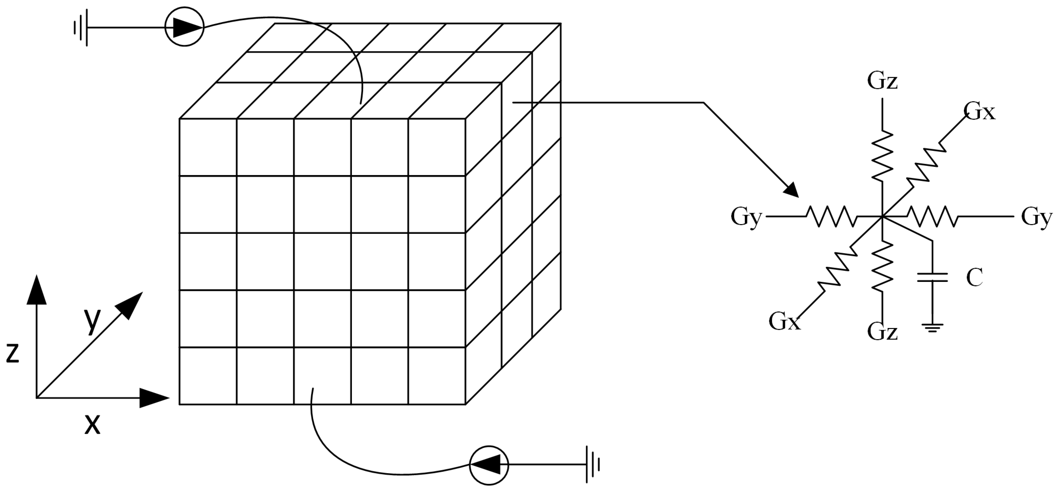
- 3D discretization of the chip: The spatial steps , in the x- and y-direction are user defined, but the step along the z-direction is typically chosen to coincide with the interface between successive layers (metal and insulator). The discretization procedure naturally covers multiple layers in the z-direction and can be easily extended to model heterogeneous structures that can be found in modern chips (e.g., heat sinks).
- Formulation of equivalent circuit description: Using modified nodal analysis, the equivalent circuit is described by the ODE system (10).
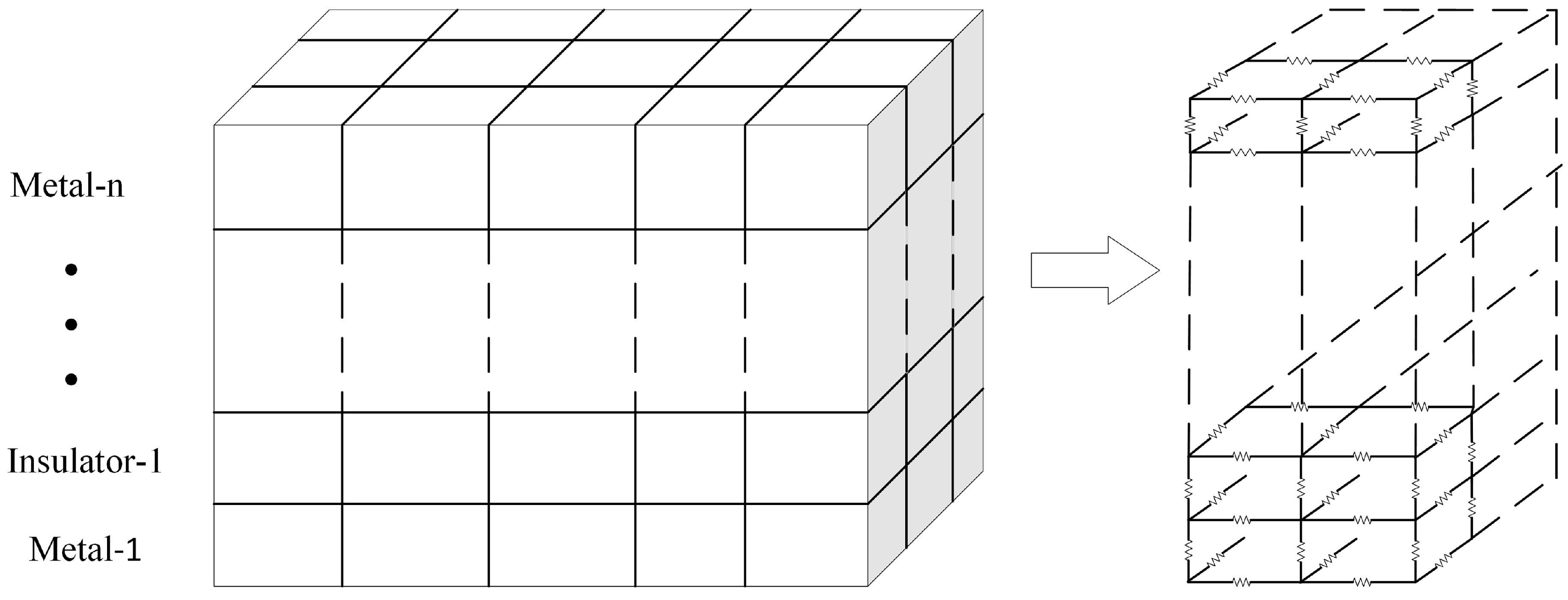
- Construction of the preconditioner matrix: Based on the algorithm described in the previous section, the preconditioner matrix is constructed based on [24], and the preconditioner-solve step is performed with the fast transform solver. More specifically, the thermal grid is equivalent to a highly regular resistive network, as depicted in Figure 2, with resistive branches connecting nodes in the x, y, and z axis. To create a preconditioner that will approximate the grid matrix, we substitute each horizontal and vertical thermal conductance with its average value in the corresponding layer. Moreover, we substitute each thermal conductance connecting nodes in adjacent layers (z axis) with their average value between the two layers.
- Compute either the DC or transient solution: The solution is obtained with the iterative PCG method in both cases. Note that in the case of the transient solution, the backward-Euler numerical integration method as in (11) is employed for the calculation of temperature in each discrete time instant. The convergence of the method is accelerated with the highly parallel fast transform solver that is used in preconditioner-solve step in Algorithm 1.
6. Experimental Results
7. Conclusions
Author Contributions
Funding
Conflicts of Interest
Abbreviations
| EDA | Electronic Design Automation |
| GPU | Graphic Processor Unit |
| IC | Integrated Circuit |
| SOI | Silicon on Insulator |
| FDM | Finite Difference Method |
| PCG | Preconditioned Conjugate Gradient |
| ICCG | Incomplete Cholesky Conjugate Gradient |
| FEM | Finite Element Method |
| ADI | Alternating Direction Implicit |
| NN | Neural Net |
| LUT | Look Up Table |
| MOR | Model Order Reduction |
| GMRES | Generalized Minimal RESidual |
| PDE | Partial Differential Equation |
| LHS | Left-Hand Side |
| MNA | Modified Nodal Analysis |
| ODE | Ordinary Differential Equations |
| SPD | Symmetric and Positive Definite |
| CG | Conjugate Gradient |
| RHS | Right-Hand Side |
| DCT-II | Discrete Cosine Transform of Type-II |
| IDCT-II | Inverse Discrete Cosine Transform of Type-II |
| FFT | Fast Fourier Transform |
| FT-PCG | Fast Transform Preconditioned Conjugate Gradient |
References
- Waldrop, M.M. The Chips Are Down for Moore’s Law. Nat. News 2016, 530, 144–147. [Google Scholar] [CrossRef] [PubMed]
- Xu, C.; Kolluri, S.K.; Endo, K.; Banerjee, K. Analytical Thermal Model for Self-Heating in Advanced FinFET Devices with Implications for Design and Reliability. IEEE Trans. Comput. Aided Des. Integr. Circuits Syst. 2013, 32, 1045–1058. [Google Scholar]
- SIA. International Technology Roadmap for Semiconductors (ITRS) 2015 Edition-ERD; SIA: Washington, DC, USA, 2015. [Google Scholar]
- Pedram, M.; Nazarian, S. Thermal modeling, analysis, and management in VLSI circuits: Principles and methods. Proc. IEEE 2006, 94, 1487–1501. [Google Scholar] [CrossRef]
- Floros, G.; Daloukas, K.; Evmorfopoulos, N.; Stamoulis, G. A parallel iterative approach for efficient full chip thermal analysis. In Proceedings of the 7th International Conference on Modern Circuits and Systems Technologies (MOCAST), Thessaloniki, Greece, 7–9 May 2018; pp. 1–4. [Google Scholar]
- Li, P.; Pileggi, L.T.; Asheghi, M.; Chandra, R. Efficient full-chip thermal modeling and analysis. In Proceedings of the IEEE/ACM International Conference on Computer Aided Design, San Jose, CA, USA, 7–11 November 2004; pp. 319–326. [Google Scholar]
- Li, P.; Pileggi, L.T.; Asheghi, M.; Chandra, R. IC thermal simulation and modeling via efficient multigrid-based approaches. IEEE Trans. Comput. Aided Des. Integr. Circuits Syst. 2006, 25, 1763–1776. [Google Scholar]
- Yang, Y.; Zhu, C.; Gu, Z.; Shang, L.; Dick, R.P. Adaptive multi-domain thermal modeling and analysis for integrated circuit synthesis and design. In Proceedings of the IEEE/ACM International Conference on Computer Aided Design, San Jose, CA, USA, 5–9 November 2006; pp. 575–582. [Google Scholar]
- Yang, Y.; Gu, Z.; Zhu, C.; Dick, R.P.; Shang, L. ISAC: Integrated Space-and-Time-Adaptive Chip-Package Thermal Analysis. IEEE Trans. Comput. Aided Des. Integr. Circuits Syst. 2007, 26, 86–99. [Google Scholar] [CrossRef] [Green Version]
- Wang, T.Y.; Chen, C.C.P. 3-D Thermal-ADI: A linear-time chip level transient thermal simulator. IEEE Trans. Comput. Aided Des. Integr. Circuits Syst. 2002, 21, 1434–1445. [Google Scholar] [CrossRef]
- Sridhar, A.; Vincenzi, A.; Ruggiero, M.; Brunschwiler, T.; Atienza, D. 3D-ICE: Fast compact transient thermal modeling for 3D ICs with inter-tier liquid cooling. In Proceedings of the IEEE/ACM International Conference on Computer-Aided Design, San Jose, CA, USA, 7–11 November 2010; pp. 463–470. [Google Scholar]
- Sridhar, A.; Vincenzi, A.; Atienza, D.; Brunschwiler, T. 3D-ICE: A Compact Thermal Model for Early-Stage Design of Liquid-Cooled ICs. IEEE Trans. Comput. 2014, 63, 2576–2589. [Google Scholar] [CrossRef] [Green Version]
- Ladenheim, S.; Chen, Y.C.; Mihajlovic, M.; Pavlidis, V. IC thermal analyzer for versatile 3-D structures using multigrid preconditioned Krylov methods. In Proceedings of the IEEE/ACM International Conference on Computer-Aided Design, Austin, TX, USA, 7–10 November 2016; pp. 1–8. [Google Scholar]
- Zhan, Y.; Sapatnekar, S.S. High-Efficiency Green Function-Based Thermal Simulation Algorithms. IIEEE Trans. Comput. Aided Des. Integr. Circuits Syst. 2007, 26, 1661–1675. [Google Scholar] [CrossRef]
- Vincenzi, A.; Sridhar, A.; Ruggiero, M.; Atienza, D. Fast thermal simulation of 2D/3D integrated circuits exploiting neural networks and GPUs. In Proceedings of the IEEE/ACM International Symposium on Low Power Electronics and Design, Fukuoka, Japan, 1–3 August 2011; pp. 151–156. [Google Scholar]
- Lee, Y.M.; Pan, C.W.; Huang, P.Y.; Yang, C.P. LUTSim: A Look-Up Table-Based Thermal Simulator for 3-D ICs. IEEE Trans. Comput. Aided Des. Integr. Circuits Syst. 2015, 34, 1250–1263. [Google Scholar]
- Wang, T.Y.; Chen, C.C.P. SPICE-compatible thermal simulation with lumped circuit modeling for thermal reliability analysis based on modeling order reduction. In Proceedings of the International Symposium on Signals, Circuits and Systems, San Jose, CA, USA, 22–24 March 2004; pp. 357–362. [Google Scholar]
- Floros, G.; Evmorfopoulos, N.; Stamoulis, G. Efficient Hotspot Thermal Simulation Via Low-Rank Model Order Reduction. In Proceedings of the 15th International Conference on Synthesis, Modeling, Analysis and Simulation Methods and Applications to Circuit Design (SMACD), Prague, Czech Republic, 2–5 July 2018; pp. 205–208. [Google Scholar]
- Liu, X.X.; Zhai, K.; Liu, Z.; He, K.; Tan, S.X.D.; Yu, W. Parallel Thermal Analysis of 3-D Integrated Circuits With Liquid Cooling on CPU-GPU Platforms. IEEE Trans. Very Large Scale Integr. Syst. 2015, 23, 575–579. [Google Scholar]
- Ouzisik, N. Heat Transfer—A Basic Approach; Mcgraw-Hill College Book Company: New York, NY, USA, 1985. [Google Scholar]
- Bergman, T.; Lavine, B.; Incropera, P.; DeWitt, P. Fundamentals of Heat and Mass Transfer; Wiley: New York, NY, USA, 2017. [Google Scholar]
- Barrett, R.; Berry, M.; Chan, T.; Demmel, J.; Donato, J.; Dongarra, J.; Eijkhout, V.; Pozo, R.; Romine, C.; van der Vorst, H. Templates for the Solution of Linear Systems: Building Blocks for Iterative Methods, 2nd ed.; SIAM: Philadelphia, PA, USA, 1992. [Google Scholar]
- Axelsson, O.; Barker, V.A. Quadratic Spline Collocation Methods for Elliptic Partial Differential Equations; Academic Press: Cambridge, MA, USA, 1984. [Google Scholar]
- Daloukas, K.; Marnari, A.; Evmorfopoulos, N.; Tsompanopoulou, P.; Stamoulis, G.I. A parallel fast transform-based preconditioning approach for electrical-thermal co-simulation of power delivery networks. In Proceedings of the Design, Automation & Test in Europe Conference & Exhibition (DATE), Grenoble, France, 18–22 March 2013; pp. 1689–1694. [Google Scholar]
- Daloukas, K.; Evmorfopoulos, N.; Tsompanopoulou, P.; Stamoulis, G. Parallel Fast Transform-Based Preconditioners for Large-Scale Power Grid Analysis on Graphics Processing Units (GPUs). IEEE Trans. Comput. Aided Des. Integr. Circuits Syst. 2016, 35, 1653–1666. [Google Scholar] [CrossRef]
- Christara, C.C. Quadratic Spline Collocation Methods for Elliptic Partial Differential Equations. BIT Numer. Math. 1994, 34, 33–61. [Google Scholar] [CrossRef]
- Van Loan, C. Computational Frameworks for the Fast Fourier Transform; SIAM: Philadelphia, PA, USA, 1992. [Google Scholar]
- NVIDIA CUDA Programming Guide, CUSPARSE, CUBLAS, and CUFFT Library User Guides. Available online: http://developer.nvidia.com/nvidia-gpu-computing-documentation (accessed on 19 December 2018).


| Electrical Circuit | Thermal Circuit |
|---|---|
| Voltage | Temperature |
| Current | Heat Flow |
| Electrical Conductance | Thermal Conductance |
| Electrical Resistance | Thermal Resistance |
| Electrical Capacitance | Thermal Capacitance |
| Current Source | Heat Source |
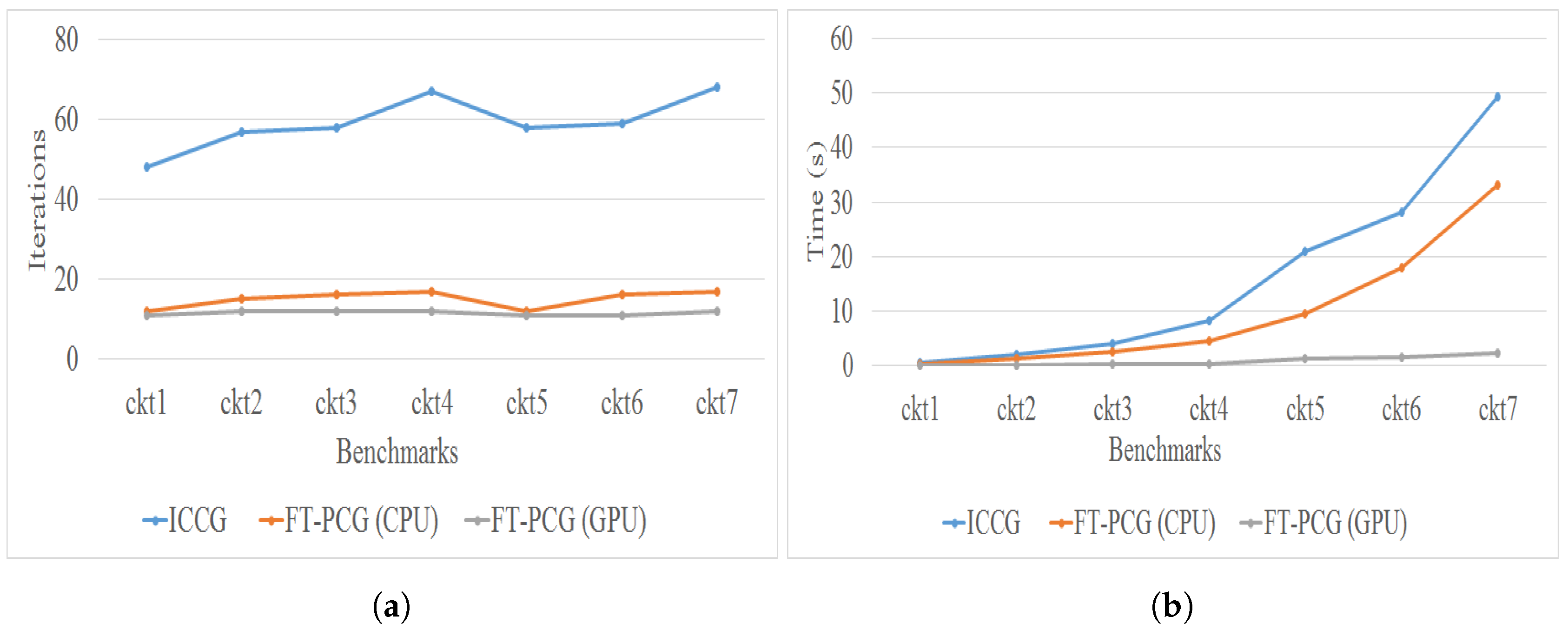
| Bench. | Discr. Points | Layers | ICCG | FT-PCG (CPU) | FT-PCG (GPU) | |||||
|---|---|---|---|---|---|---|---|---|---|---|
| Iter. | Time (s) | Iter. | Time (s) | Speedup | Iter. | Time (s) | Speedup | |||
| ckt1 | 175 | 5 | 48 | 0.48 | 12 | 0.31 | 1.54× | 11 | 0.03 | 16× |
| ckt2 | 320 | 5 | 57 | 1.98 | 15 | 1.23 | 1.6× | 12 | 0.08 | 24.75× |
| ckt3 | 410 | 6 | 58 | 4.20 | 16 | 2.64 | 1.59× | 12 | 0.23 | 18.26× |
| ckt4 | 500 | 7 | 67 | 8.35 | 17 | 4.51 | 1.85× | 12 | 0.31 | 26.93× |
| ckt5 | 845 | 7 | 58 | 21.07 | 12 | 9.48 | 2.22× | 11 | 1.34 | 15.72× |
| ckt6 | 946 | 7 | 59 | 28.27 | 16 | 17.94 | 1.57× | 11 | 1.60 | 17.65× |
| ckt7 | 1118 | 8 | 68 | 49.35 | 17 | 33.07 | 1.49× | 12 | 2.39 | 20.64× |
© 2018 by the authors. Licensee MDPI, Basel, Switzerland. This article is an open access article distributed under the terms and conditions of the Creative Commons Attribution (CC BY) license (http://creativecommons.org/licenses/by/4.0/).
Share and Cite
Floros, G.; Daloukas, K.; Evmorfopoulos, N.; Stamoulis, G. A Preconditioned Iterative Approach for Efficient Full Chip Thermal Analysis on Massively Parallel Platforms. Technologies 2019, 7, 1. https://doi.org/10.3390/technologies7010001
Floros G, Daloukas K, Evmorfopoulos N, Stamoulis G. A Preconditioned Iterative Approach for Efficient Full Chip Thermal Analysis on Massively Parallel Platforms. Technologies. 2019; 7(1):1. https://doi.org/10.3390/technologies7010001
Chicago/Turabian StyleFloros, George, Konstantis Daloukas, Nestor Evmorfopoulos, and George Stamoulis. 2019. "A Preconditioned Iterative Approach for Efficient Full Chip Thermal Analysis on Massively Parallel Platforms" Technologies 7, no. 1: 1. https://doi.org/10.3390/technologies7010001
APA StyleFloros, G., Daloukas, K., Evmorfopoulos, N., & Stamoulis, G. (2019). A Preconditioned Iterative Approach for Efficient Full Chip Thermal Analysis on Massively Parallel Platforms. Technologies, 7(1), 1. https://doi.org/10.3390/technologies7010001