A Matheuristic Optimization Approach for Simultaneous Feeder Routing and Conductor Sizing in Unbalanced Distribution Networks

Abstract

The optimal expansion of unbalanced three-phase distribution networks in non-interconnected zones requires the simultaneous resolution of two highly complex planning decisions: the selection of feeder routes and the sizing of conductors. This problem, formulated as a non-convex mixed-integer nonlinear program (MINLP), poses significant computational challenges due to the combinatorial explosion of radial topologies, discrete conductor choices, and the nonlinearity of three-phase power-flow equations. While metaheuristics offer flexible exploration, they lack optimality guarantees and repeatability, whereas exact MINLP solvers provide rigorous solutions but become computationally intractable for systems of realistic size. To overcome these limitations, this paper introduces a novel hybrid exact–metaheuristic framework that synergistically combines the global exploration capabilities of the Equilibrium Optimizer (EO) with the rigorous evaluation power of an exact MINLP model. In this cascade architecture, EO efficiently navigates the discrete space of radial topologies, while the exact MINLP stage, solved using BONMIN with an interior-point branch-and-bound scheme, optimizes conductor selection and evaluates the full annualized cost, rigorously enforcing voltage, ampacity, and physical constraints. The proposed methodology was validated on 10-, 30-, 50-, and 110-node test systems derived from real Colombian non-interconnected zones (Nuquí, Leticia, San Andrés, and a large-scale urban case). Comparative analysis against pure metaheuristics (SSA, GWO, VSA) and standalone MINLP demonstrates that EO-MINLP consistently yields the lowest total annualized costs, achieving savings of up to 0.42%, 0.71%, and 1.36% over the best pure metaheuristic for the 10-, 30-, and 50-node systems, respectively. Crucially, the hybrid strategy dramatically enhances scalability, reducing the standalone MINLP computational time by 15.79%, 78.68%, and 88.95% for these cases, while preserving solution quality and improving repeatability (standard deviation reduced from over 1.2% to as low as 0.11%). For the challenging 110-node system, where the standalone MINLP proved computationally infeasible, the proposed method successfully delivered a feasible, high-quality solution with a standard deviation of just 0.43%, confirming its practical applicability to large-scale planning. These results demonstrate that the EO-MINLP framework provides a robust, scalable, and economically superior tool for the cost-effective design of unbalanced distribution networks, effectively bridging the gap between the flexibility of stochastic search and the rigor of mathematical programming.

1. Introduction

1.1. General Context and Problem Characterization

The expansion and modernization of electrical distribution networks (EDNs) are pivotal to achieving universal access to reliable, affordable, and sustainable energy, particularly in developing economies and isolated regions [1]. Within this context, non-interconnected zones (ZNIs) present a significant challenge: these areas operate independently of the main national grid, often relying on costly local generation and facing severe constraints in infrastructure investment, operational efficiency, and technical performance [2,3]. The planning of EDNs in such environments must reconcile the need for spatial coverage (feeder routing) with the appropriate sizing of conductors, all while ensuring long-term economic viability and adherence to strict operational limits [4,5].

The problem of simultaneously selecting the optimal set of routes (i.e., a radial topology) and the conductor calibers for each branch is inherently complex [6]. It constitutes a mixed-integer nonlinear programming (MINLP) formulation characterized by three compounding sources of difficulty: (i) a discrete combinatorial explosion from the exponential number of possible radial tree structures, (ii) a discrete set of conductor sizes per line, and (iii) a set of nonlinear, non-convex three-phase power-flow equations that govern voltage drops, current flows, and power losses [7]. Furthermore, the unbalanced nature of distribution systems—caused by asymmetrical loads, untransposed lines, and single-phase laterals—requires a full three-phase representation, eliminating the simplifying assumptions of balanced models and further increasing the problem’s numerical stiffness [8,9]. Traditional solution paradigms, whether purely metaheuristic or purely exact, face substantial limitations when addressing this problem at a realistic scale.

1.2. Motivation and Scientific Gap

The primary motivation for this work stems from the inadequacy of conventional solution strategies when applied to the joint route and conductor selection problem in unbalanced systems of practical size. Purely metaheuristic approaches, such as Genetic Algorithms, Particle Swarm Optimization, Grey Wolf Optimizer (GWO), Salp Swarm Algorithm (SSA), or Vortex Search Algorithm (VSA), are widely adopted due to their flexibility, derivative-free nature, and ability to navigate large, discrete-continuous search spaces [10,11,12,13]. However, their performance is inherently stochastic. The final solution quality depends heavily on parameter tuning, initialization, and random sampling, leading to variability across independent runs and a lack of repeatability. Moreover, these methods provide no optimality gap, making it impossible to ascertain how far a given solution is from the global optimum [14,15,16].

Conversely, exact optimization methods, including MINLP solvers that combine branch-and-bound with interior-point methods, offer deterministic convergence and the ability to certify optimality (or provide a proven optimality gap) [17,18,19,20]. Their principal drawback is computational intractability for large-scale instances. As the number of nodes, candidate lines, and conductor options increases, the branch-and-bound tree expands explosively, and solving the continuous nonlinear relaxations at each node becomes computationally dominant [7]. This often restricts exact methods to small or medium-sized systems (e.g., up to 30 nodes) and makes them impractical for real-world urban or semi-urban networks with 50 or more nodes [21]. The scientific gap, therefore, lies in the lack of a scalable solution framework that preserves the rigor of exact electrical modeling and discrete optimization while achieving the computational efficiency required for larger, operationally realistic unbalanced distribution systems.

1.3. State-of-the-Art and Critical Literature Review

The existing literature on distribution system planning can be broadly categorized into three streams: metaheuristic-only, exact-only, and hybrid approaches.

1.3.1. Metaheuristic Approaches

Metaheuristic approaches dominate the literature due to their relative ease of implementation and their ability to handle discrete-continuous planning variables. Dash et al. [10] formulated a multi-objective planning problem for the simultaneous allocation of multitype DGs and D-STATCOMs, considering real power losses, voltage deviation, voltage stability, and annual cost. Their work shows that population-based algorithms can effectively address distribution planning problems involving technical and economic objectives.

Similarly, Shaikh et al. [11] proposed a Black Widow Optimization-based approach for the simultaneous sizing and placement of DGs and DSTATCOMs in radial distribution networks. The results obtained in IEEE 12-, 33-, and 69-bus systems showed significant reductions in active and reactive power losses, as well as improvements in voltage profiles, confirming the suitability of metaheuristics for device-placement problems in distribution systems.

Other studies have focused on topology-related decisions. Kerckhove et al. [12] compared metaheuristic and mathematical programming approaches for low-voltage network reconfiguration, showing the computational advantage of genetic algorithms in networks with large combinatorial search spaces. Likewise, Huy et al. [13] proposed a chaotic search group algorithm for simultaneous network reconfiguration and distributed generation allocation, demonstrating improvements in power loss reduction and voltage profiles in 33-, 69-, 84-, and 118-bus radial distribution systems.

Recent studies have also extended metaheuristic optimization to emerging planning problems associated with electric mobility and active loads. For instance, Fotis [22] proposed a Binary Random Dynamic Arithmetic Optimization Algorithm for the optimal placement and sizing of electric vehicle charging stations in an IEEE 33-bus distribution system. The study considered voltage behavior, active power demand, and system losses, showing that improved metaheuristic strategies can reduce active power losses and computational effort when compared with conventional arithmetic optimization and other metaheuristic algorithms.

More recent advances have explored variants of the Equilibrium Optimizer (EO), which mimics a dynamic mass balance model to balance exploration and exploitation [23]. Improved EO variants have been proposed to enhance convergence speed, search accuracy, and the ability to avoid local optima [24,25,26]. These developments support the use of EO as a competitive optimizer for complex nonlinear and combinatorial problems.

Despite these advances, most existing metaheuristic-based studies focus on the placement and sizing of active or reactive devices, electric vehicle charging stations, or network reconfiguration in predefined radial networks. In contrast, the simultaneous selection of feeder routes and conductor calibers in unbalanced three-phase distribution networks remains less explored. Moreover, many approaches evaluate candidate solutions using power-flow routines embedded within the metaheuristic loop, whereas the proposed EO-MINLP framework combines stochastic topology exploration with an exact conductor-sizing stage under detailed three-phase nonlinear operational constraints.

1.3.2. Exact Optimization Approaches

Exact optimization approaches have gained relevance due to the increasing maturity of commercial and open-source mathematical programming solvers. Gallego et al. [17] formulated the integrated distribution network reconfiguration and conductor selection problem as a mixed-integer linear programming (MILP) model. Their work is relevant because it jointly considers topology modification and conductor selection in a single optimization framework, showing that simultaneous planning decisions can outperform sequential or isolated strategies. However, the formulation relies on a single-phase equivalent and linearized power-flow expressions, which limits its applicability to unbalanced three-phase networks with explicit phase coupling.

Ayazi et al. [18] proposed an MILP model for the optimal operation of unbalanced distribution networks through coordinated network reconfiguration and soft open points. Their contribution is particularly important because it considers phase-specific operation; mutual impedances; single-, double-, and three-phase branches; and voltage imbalance mitigation. Nevertheless, the study focuses on operational reconfiguration and SOP utilization rather than long-term infrastructure expansion decisions such as feeder routing and conductor sizing.

Full MINLP formulations provide a more detailed representation of nonlinear physical phenomena, but they also increase computational complexity. Herkenrath et al. [19] showed that MINLP problems with continuous and discrete decisions can be addressed using either metaheuristic or gradient-based optimization strategies, emphasizing the trade-off between flexibility and computational efficiency. Similarly, Li et al. [20] proposed a feasibility-pump strategy for large-scale MINLP problems arising from AC optimal power flow with unit-commitment variables, showing that decomposition and relaxation-based strategies can improve tractability in highly nonlinear power-system applications.

In the specific context of feeder routing and conductor sizing, Cortés-Caicedo et al. [9] formulated the problem as a non-convex MINLP in complex variables for unbalanced three-phase distribution systems. This formulation preserves three-phase voltage-current-power couplings and explicitly includes radiality, voltage, ampacity, and conductor-selection constraints. However, the standalone MINLP approach becomes computationally demanding as the system size increases, requiring long solution times for medium-size test systems and becoming practically prohibitive for larger instances.

From an algorithmic perspective, the branch-and-bound framework remains the core mechanism behind many exact mixed-integer optimization methods. Morrison et al. [27] explain that branch-and-bound systematically explores the discrete search space through branching, bounding, and pruning strategies. Although this structure can provide optimality certificates under suitable convexity and bounding conditions, its computational burden grows rapidly with the number of binary variables, especially when each node of the search tree requires solving nonlinear continuous relaxations.

Overall, the reviewed exact optimization studies show that MILP and convexified models provide strong computational advantages and, in many cases, global optimality guarantees for the approximated problem. However, these benefits are usually obtained through linearizations, single-phase equivalents, or restrictions in the planning scope. On the other hand, full MINLP formulations can represent the nonlinear three-phase physics more accurately, but they face severe scalability limitations. This reveals a clear gap in the literature: the need for hybrid exact–metaheuristic strategies capable of preserving detailed unbalanced three-phase modeling while reducing the computational burden of simultaneous feeder routing and conductor sizing.

1.3.3. Hybrid Exact–Metaheuristic Strategies

Hybrid exact–metaheuristic strategies have recently emerged as a compelling alternative to bridge the gap between flexible exploration and mathematical rigor. These frameworks usually decompose the original problem into two interdependent subproblems: a master problem solved by a metaheuristic, such as topology selection or candidate asset placement, and a slave problem solved through mathematical programming, such as optimal power flow, conductor sizing, or device operation.

For example, Patiño et al. [21] proposed an exact MILP formulation for the optimal placement, sizing, and operation of D-STATCOMs in radial distribution systems. Although the method is not strictly metaheuristic–exact, it illustrates the advantages of mathematical programming for device-placement problems, particularly when multi-period operation and globally optimal solutions are required. However, the planning decision is limited to reactive compensation devices, without addressing feeder routing or conductor selection.

Useche et al. [16] proposed a robust mixed-integer second-order cone programming model for energy management in active distribution systems. Their approach coordinates reactive power resources such as capacitor banks, photovoltaic systems, wind generators, thyristor-switched capacitors, and D-STATCOMs under uncertainty in demand and renewable generation. This contribution shows how exact conic reformulations and robust optimization can improve the tractability and reliability of active distribution system operation. Nevertheless, the focus is on operational scheduling and reactive power dispatch, rather than on long-term passive infrastructure expansion.

Other hybrid frameworks, such as GA-MINLP, PSO-MILP, or metaheuristic–OPF strategies, have also been explored in transmission expansion planning, distributed generation allocation, and active distribution network operation. These methods are attractive because the metaheuristic stage can efficiently explore large discrete search spaces, while the exact stage evaluates each candidate solution with a more rigorous mathematical model. However, most of these approaches focus on the allocation of active devices or operational resources in predefined networks.

The literature shows that hybrid exact–metaheuristic strategies are effective when the planning problem contains both combinatorial and nonlinear components. However, their application to the simultaneous selection of feeder routes and conductor calibers in unbalanced three-phase distribution networks remains limited. This gap motivates the EO-MINLP framework proposed in this paper, where the Equilibrium Optimizer explores feasible radial topologies and the MINLP stage performs conductor selection under detailed three-phase operational constraints.

1.4. Novelty and Main Contributions

The novelty lies in a hybrid EO-MINLP framework that synergizes the global search of the Equilibrium Optimizer with the rigorous exactness of MINLP (BONMIN) for the simultaneous route and conductor selection problem in unbalanced three-phase distribution networks. Unlike pure metaheuristics, the exact slave stage guarantees feasibility under full non-convex power-flow, voltage, and ampacity constraints; unlike standalone MINLP, the EO master prunes the topology search space to enhance scalability. The main contributions are as follows:

• Hybrid framework and MINLP formulation: A cascade EO-MINLP decomposition where EO selects radial topologies and MINLP exactly solves conductor calibers and annualized cost, incorporating radiality constraints, three-phase branch–node balance equations, discrete conductor choices, voltage/ampacity limits, and wye/delta load models.
• Validation and scalability: Tested on 10-, 30-, and 50-node real Colombian ZNI systems (Nuquí, Leticia, San Andrés). EO-MINLP reduces computational time by up to 88.95% versus standalone MINLP, achieves 0.71%–1.36% annual savings over pure metaheuristics, and improves repeatability (standard deviation from 1.24% to 0.11%).
• Planning insights: Optimal strategy shifts with load density: rural (10 nodes) dominated by voltage regulation and feeder length; semi-urban (30 nodes) by mixed voltage-current regimes; urban (50 nodes) by loss minimization.

Note that this study focuses on greenfield expansion planning for passive distribution network planning scenarios under steady-state, peak-load conditions, assuming perfectly known demand and fixed cost parameters. In this context, the expansion problem is addressed through feeder route selection and conductor sizing, without considering active operational resources or control actions, such as distributed generation, photovoltaic systems, battery energy storage systems, reactive compensation devices, or time-dependent dispatch strategies. Therefore, the proposed model is suitable for evaluating passive infrastructure expansion decisions, while multi-period planning, demand growth, hourly load variability, load factors, renewable generation profiles, and uncertainty in generation and consumption are left for future developments.

Additionally, the methodology assumes that all candidate lines are constructible without right-of-way or land-use constraints. Although the hybrid approach significantly reduces computational time compared with the standalone MINLP formulation, its application to very large systems, e.g., 100+ nodes, may still require further decomposition or parallel computing strategies. These limitations define the boundaries of the current contribution and outline natural directions for extending the proposed framework toward active distribution network planning.

1.5. Document Structure

The remainder of this paper is organized as follows. Section 2 presents the complete MINLP formulation of the simultaneous route and conductor selection problem, including the objective function, power-flow constraints, radiality conditions, and operational limits. Section 3 describes the proposed hybrid exact–metaheuristic methodology in detail, explaining the EO for route selection, the exact MINLP solver (BONMIN) for conductor sizing, and the iterative information exchange between stages. Section 4 introduces the three unbalanced test systems (10, 30, and 50 nodes), including nodal load data, candidate line sets, conductor characteristics, and economic parameters derived from the Colombian ZNIs. Section 5 presents a comprehensive analysis of the simulation results, comparing the proposed EO-MINLP method against pure metaheuristics (SSA, GWO, VSA, EO) and the standalone MINLP formulation in terms of solution quality, repeatability, and computational effort. Finally, Section 6 concludes the paper, summarizes the main findings, and outlines directions for future research, including multi-period planning, integration of distributed energy resources, and advanced decomposition techniques.

2. General MINLP Formulation

The simultaneous route and conductor selection problem in unbalanced three-phase distribution networks is formulated as an MINLP model [8]. The objective function minimizes the total annualized cost, which comprises two main components: the cost of energy losses during system operation and the annualized investment cost of the conductors installed on each selected line [9]. The model explicitly enforces three-phase power-flow equations, radiality constraints, discrete conductor selection, voltage regulation limits, source capacity bounds, and thermal ampacity constraints. The complete mathematical formulation is presented below.

2.1. Objective Function

The objective function, given in (1), seeks to minimize the total annualized cost $f_{\mathrm{cost}}$, which is the sum of the annualized energy loss cost $f_{\mathrm{loss}}$ and the annualized conductor investment cost $f_{\mathrm{inv}}$ [9].

$$\min f_{\mathrm{cost}}=f_{\mathrm{loss}}+f_{\mathrm{inv}},$$

(1)

The annualized energy loss cost, defined in (2), quantifies the economic impact of active power dissipated as heat in the network conductors over one year. The term $f_{\alpha }(i_a,N_t)$ is the capital recovery factor, which converts a present lump sum into an equivalent uniform annual series over a planning horizon of $N_t$ years, using a discount rate $i_a$. The factor $f_{\beta }(i_a,i_e,N_t)$ converts the first-year loss cost into its present value, accounting for energy price escalation at rate $i_e$ and discounting at rate $i_a$. Thus, the product $f_{\alpha }·f_{\beta }$ directly converts the first-year loss cost into an equivalent uniform annual cost. The average energy generation cost is denoted by $C_{kWh}$, and the annual operating time is T hours, representing continuous operation at peak demand. The term $\mathrm{Re}\left\{{\sum }_{l\in \mathcal{L}}{\mathbb{V}}_{l3\phi }^{\top }{\mathbb{J}}_{l3\phi }^{\star }\right\}$ computes the total three-phase active power losses across all lines $l\in \mathcal{L}$, where ${\mathbb{V}}_{l3\phi }$ is the complex voltage vector across line l, ${\mathbb{J}}_{l3\phi }^{\star }$ is the complex conjugate of the current vector flowing through line l, and $\mathcal{L}$ is the set of candidate lines.

$$f_{\mathrm{loss}}=f_{\alpha }{f}_{\beta }{C}_{kWh}T\mathrm{Re}\left\{\sum _{l\in \mathcal{L}}{\mathbb{V}}_{l3\phi }^{\top }{\mathbb{J}}_{l3\phi }^{\star }\right\},$$

(2)

The annualized investment cost, defined in (3), captures the cost of installing conductors on the selected network routes. The capital recovery factor $f_{\alpha }$ is applied again to convert the upfront investment into an equivalent annual cost. For each candidate line l, the binary variable ${\mathbf{Y}}_{lp}$ indicates whether conductor type p (from the set $\mathcal{C}$ of available calibers) is installed. The parameter $C_p$ is the cost per kilometer of conductor type p, and $L_l$ is the length of line l in kilometers. The inner summation selects exactly one conductor type per built line, while the outer summation aggregates the investment cost across all candidate lines.

$$f_{\mathrm{inv}}=f_{\alpha }\sum _{l\in \mathcal{L}}\left(\sum _{p\in \mathcal{C}}{C}_p{L}_l{\mathbf{Y}}_{lp}\right).$$

(3)

2.2. Constraints

The proposed MINLP formulation enforces a set of physical, topological, and operational constraints. These include Kirchhoff’s laws for three-phase unbalanced systems, power–voltage relationships for wye and delta loads, Ohm’s law with discrete conductor selection, radiality conditions, source capacity bounds, voltage regulation limits, and thermal ampacity constraints. Each constraint group is detailed below.

2.2.1. Kirchhoff’s Current Law

Equation (4) enforces KCL at each node $k\in \mathcal{N}$. The left-hand side aggregates injected currents (generator, wye load, and delta load transformed via ${\mathbf{H}}^{\top }$), while the right-hand side sums incident line currents weighted by the three-phase incidence matrix ${\mathbf{A}}_{kl3\phi }$ [9].

$${\mathbb{I}}_{k3\phi }^g-{\mathbb{I}}_{k3\phi }^{dY}-{\mathbf{H}}^{\top }{\mathbb{I}}_{k3\phi }^{d\Delta }=\sum _{l\in \mathcal{L}}{\mathbf{A}}_{kl3\phi }{\mathbb{J}}_{l3\phi },\forall k\in \mathcal{N},$$

(4)

2.2.2. Power–Voltage Relationships

Equations (5)–(7) define complex power as the element-wise product of voltage and current. Generator power is given by (5), wye load power by (6), and delta load power by (7), where $\mathbf{H}$ converts line-to-neutral to line-to-line voltages [9].

$${\mathbb{S}}_{k3\phi }^{g,\star }=\mathbf{diag}\left({\mathbb{V}}_{k3\phi }^{\star }\right){\mathbb{I}}_{k3\phi }^g,\forall k\in \mathcal{N},$$

(5)

$${\mathbb{S}}_{k3\phi }^{dY,\star }=\mathbf{diag}\left({\mathbb{V}}_{k3\phi }^{\star }\right){\mathbb{I}}_{k3\phi }^{dY},\forall k\in \mathcal{N},$$

(6)

$${\mathbb{S}}_{k3\phi }^{d\Delta ,\star }=\mathbf{diag}\left(\mathbf{H}{\mathbb{V}}_{k3\phi }^{\star }\right){\mathbb{I}}_{k3\phi }^{d\Delta },\forall k\in \mathcal{N},$$

(7)

2.2.3. Ohm’s Law

Equation (8) expresses the voltage drop across line l as the difference between terminal voltages (first equality) and as the product of impedance and current (second equality). Impedance depends on conductor selection: ${\mathbf{Z}}_l=L_l{\sum }_{p\in \mathcal{C}}{\mathbf{Y}}_{lp}{\mathbb{Z}}_{p3\phi }$, where ${\mathbb{Z}}_{p3\phi }$ is the per-km impedance matrix [9].

$${\mathbb{V}}_{l3\phi }={\mathbf{Z}}_l\sum _{k\in \mathcal{N}}{\mathbf{A}}_{kl3\phi }{\mathbb{V}}_{k3\phi }=L_l\sum _{p\in \mathcal{C}}{\mathbf{Y}}_{lp}{\mathbb{Z}}_{p3\phi }{\mathbb{J}}_{l3\phi },\forall l\in \mathcal{L},$$

(8)

2.2.4. Radiality Constraints

Equations (9)–(11) enforce a radial topology. Constraint (9) ensures every node has at least one incident selected line. Constraint (10) fixes the number of selected lines to $n-1$. Constraint (11) links line selection ${\mathbf{Z}}_l$ to conductor assignment ${\mathbf{Y}}_{lp}$, forcing exactly one conductor per built line [28].

$$\sum _{l\in \mathcal{L}}\left|A_{kl3\phi }\right|{\mathbf{Z}}_l\ge 1,\forall k\in \mathcal{N},$$

(9)

$$\sum _{l\in \mathcal{L}}{\mathbf{Z}}_l=n-1,$$

(10)

$$\sum _{p\in \mathcal{C}}{\mathbf{Y}}_{lp}={\mathbf{Z}}_l,\forall l\in \mathcal{L},$$

(11)

2.2.5. Source Capacity Limits

Constraint (12) bounds generator complex power at each node. Constraint (13) sets these bounds to zero for all non-slack nodes, meaning only the substation can inject power [9].

$${\mathbb{S}}_k^{g,\min }\le {\mathbb{S}}_{k3\phi }^g\le {\mathbb{S}}_k^{g,\max },\forall k\in \mathcal{N},$$

(12)

$${\mathbb{S}}_k^{g,\min }={\mathbb{S}}_k^{g,\max }=0,\forall k\ne \mathrm{slack}\mathrm{node},$$

(13)

2.2.6. Voltage Regulation Limits

Constraint (14) imposes per-phase voltage magnitude bounds (typically 0.9–1.1 p.u.). Constraint (15) fixes the slack node voltage to the nominal value ${\mathbb{V}}_{\mathrm{nom}}$ [9].

$${\mathbf{1}}_{3\phi }{V}^{\min }\le \left|{\mathbb{V}}_{k3\phi }\right|\le {\mathbf{1}}_{3\phi }{V}^{\max },\forall k\in \mathcal{N},$$

(14)

$${\mathbb{V}}_{k3\phi }={\mathbb{V}}_{\mathrm{nom}},\forall k=\mathrm{slack}\mathrm{node},$$

(15)

2.2.7. Thermal Ampacity Constraints

Constraint (16) limits the current magnitude on each line to the ampacity of the selected conductor, preventing overheating [9].

$$\left|{\mathbb{J}}_{l3\phi }\right|\le {\mathbf{1}}_{3\phi }\sum _{p\in \mathcal{C}}{\mathbf{I}}_p^{\max }{\mathbf{Y}}_{lp},\forall l\in \mathcal{L}$$

(16)

2.3. Computational Complexity Analysis

The proposed MINLP formulation exhibits multiple sources of computational hardness, summarized in

Table 1. Sources of computational complexity in the proposed MINLP formulation.

Source	Description
Nonlinearities	Arise from three-phase power-flow equations: product of voltage and current vectors in (5)–(7), voltage drop expression in (8), and power loss term in (2) (real part of complex voltage–current products).
Non-convexities	Stem from two main features: (i) bilinear terms $\mathrm{diag}\left({\mathbb{V}}_{k3\phi }^{\star }\right){\mathbb{I}}_{k3\phi }$ in power definitions, and (ii) trigonometric relationships inherent to complex-valued AC power flow, making the feasible set non-convex.
Discrete decisions	Binary variables for line selection ${\mathbf{Z}}_l$ in (9)–(10) and conductor assignment ${\mathbf{Y}}_{lp}$ in (11) introduce combinatorial complexity. Total binary variables scales as $\left|\mathcal{L}\right|\times \left|\mathcal{C}\right|$, where $\left|\mathcal{L}\right|$ is the number of candidate lines and $\left|\mathcal{C}\right|$ is the number of conductor types.
Radiality constraints	Equations (9) and (10) impose a spanning-tree structure, restricting feasible space to a subset of the $n^{n-2}$ possible tree topologies (Cayley’s formula), where n is the number of nodes.
Problem classification	Belongs to MINLP class with non-convex continuous relaxations, for which no polynomial-time algorithm exists unless P = NP. This complexity justifies the hybrid exact–metaheuristic solution strategy proposed in Section 3, which decouples topology exploration from conductor optimization.

.

The complexity sources summarized in Table 1 show that the proposed formulation may contain multiple feasible stationary solutions due to the simultaneous presence of nonlinearities, non-convexities, and discrete decisions. Consequently, when the complete MINLP model is solved directly using a local MINLP solver, the obtained solution cannot be interpreted, in general, as a certified global optimum. Instead, it corresponds to the best feasible solution found under the adopted solver settings. This limitation motivates the use of decomposition-based strategies, such as the exact–metaheuristic approach proposed in this paper, which separates topology exploration from conductor optimization to improve the search process and identify higher-quality feasible solutions.

3. Proposed Methodology: Exact–Metaheuristic Approach

As shown in the previous section, the proposed model constitutes a highly complex optimization problem due to the combinatorial nature associated with the simultaneous selection of routes and conductors. For this reason, its solution requires a strategy capable of efficiently exploring a large discrete search space without compromising the rigor of the electrical model or the operational representation of the unbalanced three-phase system.

Solution strategies reported in the literature for this type of problem are commonly based on metaheuristic algorithms, due to their ability to handle non-convex and highly complex models with both discrete and continuous variables [10,11,12]. Their flexibility and capacity to explore large search spaces with reasonable computational effort make them attractive for network planning problems [13]. However, because they rely on stochastic processes and parameter tuning, they do not guarantee the global optimum and may exhibit variability across runs, reducing result repeatability [14,15,16].

On the other hand, exact solution methods provide a more rigorous alternative, since they can obtain optimal solutions when global optimality conditions are certified, or otherwise the best feasible solution achievable under the adopted solver settings [17,18]. Their main advantage is the delivery of unique, verifiable, and reproducible results. However, this rigor entails a high computational cost, as solution time increases significantly with system size, the number of binary variables, and model nonlinearity, which may limit their application to large-scale systems [21].

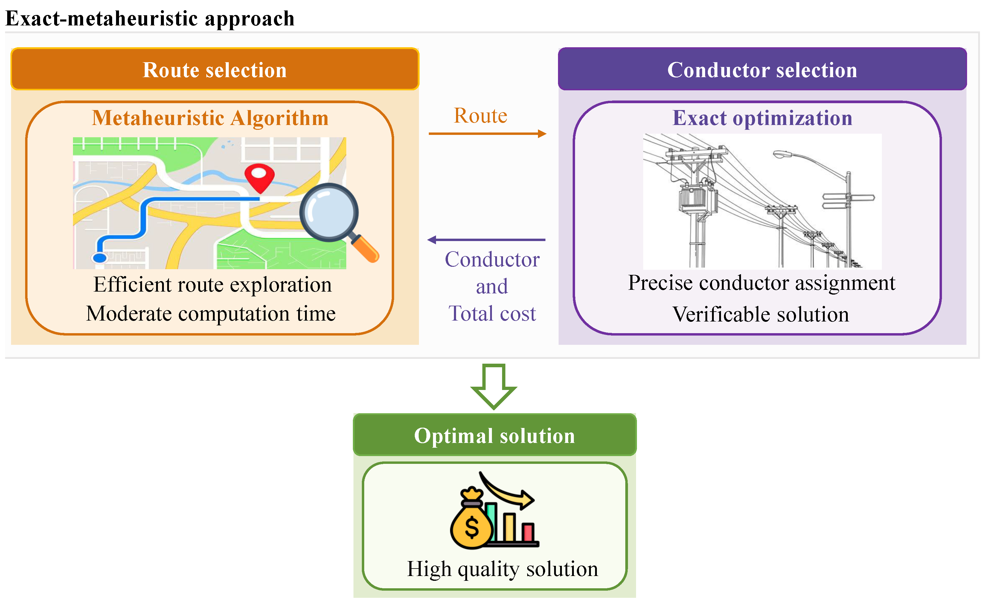
Considering the strengths and limitations of both approaches, this article proposes a hybrid methodology to address the joint problem of route and conductor selection, as shown in Figure 1.

The figure illustrates the proposed hybrid exact–metaheuristic methodology as an iterative framework in which both stages continuously exchange information. In the first stage, each metaheuristic individual proposes a candidate network topology for the route selection problem. This topology is then evaluated in the second stage through an exact optimization model, which determines the best conductor configuration and computes the objective function while enforcing all technical and operational constraints. The resulting objective value is returned to the first stage, where it guides the exploration and exploitation process to generate new candidate topologies. In this way, the methodology combines efficient global search with rigorous and reproducible solution evaluation.

This structure balances the strengths of both approaches, the metaheuristic enhances global exploration, while the exact stage reduces the variability and limited optimality guarantees of stochastic search. As a result, the proposed framework yields high-quality, optimal or near-optimal solutions with greater repeatability and lower computational burden than a fully exact solution of the complete problem.

3.1. Metaheuristic Stage: Route Selection

To address the route selection problem, this article implements the Equilibrium Optimizer (EO). The choice of this algorithm is supported by its strong numerical performance reported in the specialized literature, where it has shown competitive results against widely established metaheuristics such as Particle Swarm Optimization, Grey Wolf Optimizer, Genetic Algorithm, and Salp Swarm Algorithm [23].

EO is an algorithm inspired by the dynamic mass balance model in a control volume, where the concentration of a substance evolves according to inflow, outflow, generation, and equilibrium conditions [23,26]. Based on this analogy, EO interprets each candidate solution as a particle and its position in the search space as a concentration, so that the optimization process is modeled as a gradual transition toward an equilibrium state representing the optimal solution [24]. Under this formulation, particle updating combines three fundamental components: a reference toward high-quality solutions, a term associated with the difference with respect to the equilibrium state, and a generation term that contributes to balancing the global exploration and local exploitation of the search space [23,25].

This behavior can be mathematically modeled as explained below.

3.1.1. Initial Population

To initiate the search process, EO generates the initial individuals or concentrations, randomly within the solution space, thereby ensuring population diversity from the outset of the optimization procedure. Each individual i, or concentration i, is encoded as follows:

$$\begin{array}{c}\hfill C_i^t=\left[\begin{array}{ccccccc}1,& 2,& 3,& \cdots ,& 20,& \cdots ,& N_l\end{array}\right]\forall i=1,2,3,\cdots ,N_i\end{array}$$

where $C_i^t$ represents concentration i at iteration t, and $N_i$ is the number of individuals or concentrations that make up the population. As can be seen, each concentration i is represented by a vector of size $n-1$, corresponding to the number of active lines. Each position in this vector stores an integer associated with a candidate line, indexed from 1 to the total number of candidate lines $N_l$.

To ensure a valid radial topology, a route feasibility algorithm based on graph connectivity and spanning-tree verification is applied, following the principles described in [8]. For completeness and reproducibility, the procedure is summarized in Algorithm 1.

The purpose of this algorithm is to transform each candidate solution generated by EO into a feasible radial topology before it is evaluated by the exact conductor-selection stage. In this context, each EO concentration is encoded as a vector of candidate line indices. Since the EO position-update mechanism may generate repeated line indices, disconnected configurations, or topologies containing cycles, a feasibility verification step is required.

The algorithm first removes duplicated line indices and constructs an undirected graph $\left(G(\mathcal{N},{\mathcal{T}}_i)\right)$ using the remaining selected routes. Then, the graph is checked to verify whether all demand nodes are connected to the substation node. In addition, the number of selected branches is forced to be exactly $n-1$. These two conditions are sufficient to guarantee radiality: according to graph theory, a connected undirected graph with n nodes and $n-1$ branches is a tree [29,30]. Therefore, it cannot contain meshes, cycles, or isolated sub-loops. If the candidate graph is disconnected, the algorithm adds feasible candidate lines that connect different components. If the graph contains more than $n-1$ branches, redundant branches associated with cycles are removed. Thus, the procedure terminates only when the selected topology is connected and has exactly $n-1$ branches, ensuring that only feasible radial configurations are passed to the exact MINLP stage.

After initialization, each concentration is evaluated through the objective function in Stage 2. The population is then sorted from the individual with the best objective function value to the one with the worst, in order to identify the equilibrium candidates [23].

3.1.2. Equilibrium Pool and Candidates

Once the population has been evaluated and sorted according to the objective function value, EO selects a set of high-quality solutions referred to as the equilibrium pool. This set is composed of the four best concentrations found up to the current iteration, together with a fifth concentration computed as the arithmetic mean of those solutions [24]. Mathematically, the equilibrium pool is defined as follows:

$$C_{eq,pool}=\left\{C_{eq\left(1\right)},C_{eq\left(2\right)},C_{eq\left(3\right)},C_{eq\left(4\right)},C_{eq\left(ave\right)}\right\}$$

(17)

where $C_{eq\left(1\right)}$, $C_{eq\left(2\right)}$, $C_{eq\left(3\right)}$, and $C_{eq\left(4\right)}$ represent the four best concentrations in the population, while $C_{eq\left(ave\right)}$ corresponds to their arithmetic mean, computed as follows:

$$C_{eq\left(ave\right)}={\displaystyle \frac{C_{eq\left(1\right)}+C_{eq\left(2\right)}+C_{eq\left(3\right)}+C_{eq\left(4\right)}}{4}}$$

(18)

The incorporation of multiple equilibrium candidates, instead of a single best solution, enriches the search process by providing several high-quality references for particle updating [23]. At each iteration, each concentration randomly selects one of the elements from the equilibrium pool to guide its movement through the search space, thereby promoting a suitable balance between diversification and intensification in the optimization process.

3.1.3. Updating the Position of Each Concentration

Once the equilibrium pool has been defined, each concentration updates its position in the search space by taking as reference one of the equilibrium candidates selected at random. This process is modeled through an update equation that combines three components: the equilibrium concentration, a term associated with the difference between the current concentration and the equilibrium state, and a generation term that contributes to refining the search. Accordingly, the new position of each concentration is obtained as follows:

$$C_i^{t+1}=C_{eq}+\left(C_i^t-C_{eq}\right)\odot F+{\displaystyle \frac{G}{\lambda V}}\odot (1-F),$$

(19)

where $C_i^t$ and $C_i^{t+1}$ represent concentration i at iterations t and $t+1$, respectively; $C_{eq}$ is the equilibrium candidate selected from the equilibrium pool; F is the exponential control term; G is the generation rate; $\lambda$ is the turnover-rate vector; and V is the control volume, which is assumed to be unitary in the algorithm implementation.

The exponential term F is defined as follows:

$$F=a_1\mathrm{sign}(r-0.5)\odot \left(e^{-\lambda t}-1\right),$$

(20)

where $a_1$ is a parameter that regulates the exploration capability of the algorithm, and r is a random vector in the interval $[0,1]$. In turn, the generation rate is computed as follows:

$$G=G_0\odot F,$$

(21)

with

$$G_0=GCP\odot \left(C_{eq}-\lambda \odot C_i^t\right),$$

(22)

where $GCP$ is a control parameter that activates or deactivates the contribution of the generation term during the update process. Altogether, this formulation allows each concentration to combine global exploration and local exploitation movements, progressively guiding the population toward higher-quality regions in the solution space.

3.1.4. Updating the Equilibrium Pool

After updating the position of each concentration and re-evaluating the population through the objective function in Stage 2, the equilibrium pool is updated. In this implementation, the update is performed using an elitist criterion. First, the population is sorted according to the objective function value, from the best concentration to the worst one. Then, the first four concentrations of the current population are compared with the four candidates stored in the equilibrium pool. Each candidate is replaced only if the corresponding concentration in the current iteration exhibits a better objective function value.

Mathematically, this updating rule can be expressed as

$$C_{eq\left(j\right)}^{t+1}=\left\{\begin{array}{cc}\hfill C_{\left(j\right)}^{t+1},\hfill & \mathrm{if}f\left(C_{\left(j\right)}^{t+1}\right)<f\left(C_{eq\left(j\right)}^t\right),\hfill \\ \hfill C_{eq\left(j\right)}^t,\hfill & \mathrm{otherwise},\hfill \end{array}\right.j=1,2,3,4$$

(23)

where $C_{\left(j\right)}^{t+1}$ denotes the j-th best concentration in the population at iteration $t+1$, while $C_{eq\left(j\right)}^t$ represents the j-th equilibrium candidate stored in the pool from the previous iteration.

This procedure ensures that the equilibrium pool preserves only solutions of equal or better quality throughout the iterative process.

3.1.5. Stopping Criterion

The proposed solution methodology adopts a single stopping criterion based on the maximum number of iterations. Accordingly, the iterative process continues until the predefined iteration limit is reached, at which point the algorithm is terminated and the best solution stored in the equilibrium pool is reported as the final solution.

3.2. Exact Stage: Conductor Selection

Once the metaheuristic stage proposes a candidate radial topology, its quality is evaluated by exactly solving the conductor selection problem, which is formulated according to the following mathematical structure:

$$\begin{array}{cc}\mathbf{Obj}.\mathbf{Func}.:& \min \left(1\right),\hfill \\ \hfill \mathbf{Subject}\mathbf{to}.:& \left(4\right)–\left(7\right), \mathrm{and} \left(12\right)–\left(16\right),\hfill \\ \hfill & \sum _{p\in \mathcal{C}}{\mathbf{Y}}_{lp}=1,\forall \left\{l\in \mathcal{L}\right\}\hfill \\ \hfill & {\mathbb{V}}_{l3\phi }=\sum _{k\in \mathcal{N}}{\mathbf{A}}_{kl3\phi }{\mathbb{V}}_{k3\phi }=L_l\sum _{p\in \mathcal{C}}{\mathbf{Y}}_{lp}{\mathbb{Z}}_{p3\phi }{\mathbb{J}}_{l3\phi },\forall \left\{\begin{array}{c}l\in \mathcal{L}\end{array}\right\}\hfill \end{array}$$

At this stage, the topology remains fixed, and the model determines the optimal conductor assignment over the active lines by minimizing the equivalent annual cost while simultaneously ensuring compliance with all technical constraints of the system. This stage is formulated as a MINLP problem, whose solution is obtained by combining a branch-and-bound scheme, responsible for handling the binary variables associated with conductor selection, with an interior-point method used to solve the nonlinear continuous relaxations that arise at each node of the search tree [19,20].

• Branch-and-bound: The branch-and-bound (B&B) scheme constitutes the core exact mechanism for handling discrete decisions in the conductor selection problem. In this work, the binary variables associated with the choice of conductor size on each active line generate a large combinatorial search space, whose exhaustive enumeration is computationally impractical. To overcome this difficulty, B&B organizes the search through a tree structure in which each node represents a partial assignment of the binary variables [27].
  At each branching step, a discrete variable is fixed to mutually exclusive values, thereby generating more restricted subproblems. For each of these nodes, a continuous relaxation of the model is solved, and its solution provides a lower bound on the best objective value achievable within that branch [27]. If this bound does not improve the best feasible solution currently known, or if the subproblem is infeasible, the corresponding branch is pruned from the tree. Otherwise, the branching process continues recursively. In this way, B&B enables a systematic exploration of the discrete solution space, while discarding unpromising regions at an early stage and significantly reducing the computational effort required to identify an optimal solution or the best feasible solution attainable.
• Interior-point method: At each node of the B&B tree, the resulting relaxation preserves the nonlinear structure of the model and must therefore be solved as an NLP problem. For this purpose, an interior-point method (IPM) is employed, which is particularly suitable for large-scale problems with nonlinear constraints and multiple inequalities. The principle of this method consists of traversing the feasible region from its interior by incorporating barrier functions that penalize proximity to the constraint boundaries [31,32]. Throughout the iterative process, the IPM solves the continuous system associated with the Karush–Kuhn–Tucker optimality conditions and simultaneously updates the primal and dual variables, following a central path that converges to a feasible stationary point. As a result, the solutions of the continuous relaxations not only provide informative bounds for the pruning process in B&B, but they also ensure technical consistency in the evaluation of each candidate topology.

The integration of B&B and IPM makes it possible to solve the exact conductor selection stage in a rigorous manner. While B&B efficiently handles the discrete nature of the problem and bounds the combinatorial search space, IPM optimizes the continuous part while preserving the operation of the electrical system. This complementarity makes a suitable tool for evaluating each topology proposed by the metaheuristic stage, providing feasible, reproducible, and high-quality solutions that serve as the basis for feedback within the overall iterative process.

4. Unbalanced Three-Phase Test Systems

To assess the performance of the proposed hybrid methodology, three test systems are considered. These systems were randomly generated following the procedure described in [8]. To validate the methodology under different operating conditions, three Colombian Non-Interconnected Zones (ZNI) were used as reference: Nuquí (Chocó), Leticia (Amazonas), and San Andrés Island. These ZNIs were selected to evaluate the methodology in settings with different scales and demand structures, representative of rural, semi-urban, and urban environments. These contexts differ in the number of users, load density, and consumption patterns, thereby imposing distinct technical and economic requirements on network planning and operation.

Accordingly, three random scenarios inspired by these ZNIs were constructed, each with a different size and demand density: a 10-node system representing a low-density rural environment (Nuquí), a 30-node system representing a medium-density semi-urban environment (Leticia), and a 50-node system representing a high-density urban environment (San Andrés). This approach enables a controlled analysis of the robustness and scalability of the proposed methodology while preserving key operational features of the ZNIs and capturing the progressive increase in combinatorial and operational complexity as the number of nodes and planning decisions grows.

Finally, it is important to mention that the load sizing in the test systems was carried out using historical data from the Institute for the Planning and Promotion of Energy Solutions for Non-Interconnected Areas (IPSE), updated in January 2026 [2].

4.1. 10-Node Distribution System: Nuquí, Chocó

For this test system, a 10-node distribution network supplied at 11.4 kV line-to-line from substation node (node 1) was considered, with nine load buses, a maximum of 258 users per node, and an average density of 50 users/km². The total active and reactive power consumption is 81 kW and 28 kvar for phase A, 228 kW and 75 kvar for phase B, and 301 kW and 103 kvar for phase C. In addition, the route planning stage considers 17 candidate line sections for possible construction, as depicted in Figure 2.

Table 2. Nodal three-phase load demand profile for the 10-node distribution system.

Node i	${\mathit{P}}_{\mathit{iA}}$	${\mathit{Q}}_{\mathit{iA}}$	${\mathit{P}}_{\mathit{iB}}$	${\mathit{Q}}_{\mathit{iB}}$	${\mathit{P}}_{\mathit{iC}}$	${\mathit{Q}}_{\mathit{iC}}$	Type
1	0	0	0	0	0	0	–
2	2	1	0	0	47	16	Y
3	0	0	16	6	31	10	$\Delta$
4	28	10	0	0	58	20	Y
5	0	0	13	4	35	12	Y
6	0	0	53	17	30	10	Y
7	29	10	53	17	0	0	Y
8	0	0	33	10	45	16	Y
9	22	7	60	21	0	0	$\Delta$
10	0	0	0	0	55	19	$\Delta$

Power quantities are reported in kilowatts (kW) and kilovolt-amperes reactive (kvar).

and

Table 3. Candidate distribution routes in the 10-node system.

Line (Connection)	Length (m)	Line (Connection)	Length (m)
1 (1–2)	1709.0097	10 (5–6)	2197.6817
2 (1–3)	3677.7065	11 (6–7)	2131.4401
3 (1–4)	3398.0402	12 (7–8)	1749.8846
4 (2–4)	2602.8609	13 (7–9)	1144.4204
5 (2–5)	2374.9907	14 (7–10)	2056.0635
6 (3–4)	2460.1809	15 (8–9)	1837.3269
7 (3–6)	3615.1239	16 (8–10)	1815.0716
8 (4–5)	2910.2251	17 (9–10)	1047.0076
9 (4–6)	1201.0117

summarize the main parametric information of the 10-node test system, including the nodal load data and the list of candidate lines considered for network construction.

4.2. 30-Node Distribution System: Leticia, Amazonas

For this test system, a 30-node distribution network supplied at 11.4 kV line-to-line from substation node (node 1) was considered, with 29 load buses, a maximum of 160 users per node, and an average density of 160 users/km². The total active and reactive power consumption is 1571 kW and 364 kvar for phase A, 945 kW and 216 kvar for phase B, and 1266 kW and 294 kvar for phase C. In addition, the route planning stage considers 55 candidate line sections for possible construction, as depicted in Figure 3.

Table 4. Nodal three-phase load demand profile for the 30-node distribution system.

Node i	${\mathit{P}}_{\mathit{iA}}$	${\mathit{Q}}_{\mathit{iA}}$	${\mathit{P}}_{\mathit{iB}}$	${\mathit{Q}}_{\mathit{iB}}$	${\mathit{P}}_{\mathit{iC}}$	${\mathit{Q}}_{\mathit{iC}}$	Type
1	0	0	0	0	0	0	–
2	78	18	0	0	47	10	Y
3	22	5	0	0	21	5	$\Delta$
4	65	16	0	0	111	26	Y
5	57	13	97	23	59	12	Y
6	78	17	84	19	0	0	$\Delta$
7	78	16	0	0	27	7	$\Delta$
8	112	28	0	0	76	16	$\Delta$
9	0	0	0	0	2	0	$\Delta$
10	113	26	51	11	57	13	$\Delta$
11	75	16	70	16	0	0	Y
12	0	0	117	26	0	0	$\Delta$
13	47	10	0	0	0	0	$\Delta$
14	97	24	81	19	0	0	Y
15	0	0	0	0	99	24	$\Delta$
16	92	19	7	1	83	19	Y
17	118	26	0	0	19	5	Y
18	50	12	0	0	0	0	Y
19	0	0	93	21	0	0	Y
20	0	0	83	20	0	0	Y
21	82	20	66	14	32	7	$\Delta$
22	66	16	0	0	117	27	$\Delta$
23	113	28	32	8	32	8	$\Delta$
24	103	24	0	0	112	27	$\Delta$
25	95	24	15	4	84	18	$\Delta$
26	0	0	58	13	0	0	$\Delta$
27	0	0	0	0	116	28	Y
28	0	0	0	0	51	12	$\Delta$
29	24	5	0	0	121	30	$\Delta$
30	6	1	91	21	0	0	$\Delta$

Power quantities are reported in kilowatts (kW) and kilovolt-amperes reactive (kvar).

and

Table 5. Candidate distribution routes in the 30-node system.

Line (Connection)	Length (m)	Line (Connection)	Length (m)
1 (1–2)	321.0685	29 (13–20)	1983.3310
2 (1–3)	381.0774	30 (13–22)	1666.8101
3 (1–4)	533.0000	31 (13–24)	1402.6707
4 (2–3)	699.0772	32 (14–16)	521.9703
5 (2–4)	655.6417	33 (14–21)	761.2253
6 (2–7)	1974.5422	34 (15–21)	1396.6474
7 (3–4)	551.6348	35 (15–29)	1844.3969
8 (3–6)	1259.6051	36 (16–23)	504.0575
9 (4–5)	813.7629	37 (16–26)	912.0291
10 (4–6)	855.0287	38 (17–18)	497.0091
11 (5–6)	470.2723	39 (19–24)	642.1410
12 (5–8)	1239.2320	40 (19–25)	699.0422
13 (6–8)	1622.6213	41 (20–22)	524.2232
14 (7–10)	1692.1504	42 (20–27)	1585.4148
15 (7–11)	2030.1576	43 (21–23)	587.0545
16 (8–9)	565.1548	44 (21–26)	791.6009
17 (9–12)	1073.2963	45 (21–29)	1702.0106
18 (9–14)	1346.6974	46 (21–30)	2094.3269
19 (10–11)	1081.5272	47 (22–27)	1074.4645
20 (10–15)	$1474.3948$	48 (23–26)	$458.9172$
21 (10–17)	$1728.2604$	49 (24–25)	$117.8007$
22 (10–18)	$1436.4157$	50 (24–28)	$717.2789$
23 (11–17)	$779.1925$	51 (25–27)	$1360.6719$
24 (11–18)	$791.2225$	52 (25–28)	$716.8068$
25 (12–14)	$792.9420$	53 (26–28)	$1218.5253$
26 (12–15)	$921.7033$	54 (26–30)	$1817.1431$
27 (13–16)	$1311.1770$	55 (29–30)	$1292.9288$
28 (13–19)	$825.1364$

summarize the main parametric information of the 30-node test system, including the nodal load data and the list of candidate lines considered for network construction.

4.3. 50-Node Distribution System: San Andres Island

For this test system, a 50-node distribution network supplied at 13.2 kV line-to-line from substation node (node 1) was considered, with 49 load buses, a maximum of 130 users per node, and an average density of 300 users/km². The total active and reactive power consumption is 2464 kW and 618 kvar for phase A, 3665 kW and 920 kvar for phase B, and 2339 kW and 587 kvar for phase C. In addition, the route planning stage considers 90 candidate line sections for possible construction, as depicted in Figure 4.

Table 6. Nodal three-phase load demand profile for the 50-node distribution system.

Node i	${\mathit{P}}_{\mathit{iA}}$	${\mathit{Q}}_{\mathit{iA}}$	${\mathit{P}}_{\mathit{iB}}$	${\mathit{Q}}_{\mathit{iB}}$	${\mathit{P}}_{\mathit{iC}}$	${\mathit{Q}}_{\mathit{iC}}$	Type
1	0	0	0	0	0	0	$\Delta$
2	0	0	0	0	142	36	$\Delta$
3	148	37	3	1	142	36	$\Delta$
4	43	11	138	35	0	0	$\Delta$
5	212	53	89	22	115	29	$\Delta$
6	88	22	0	0	123	31	Y
7	159	40	0	0	0	0	Y
8	0	0	208	52	0	0	$\Delta$
9	0	0	190	48	156	39	Y
10	0	0	0	0	77	19	$\Delta$
11	0	0	124	31	5	1	$\Delta$
12	0	0	67	17	0	0	Y
13	62	16	76	19	0	0	Y
14	0	0	136	34	0	0	$\Delta$
15	158	40	0	0	0	0	Y
16	0	0	170	43	192	48	$\Delta$
17	92	23	108	27	0	0	$\Delta$
18	59	15	171	43	0	0	$\Delta$
19	0	0	0	0	72	18	Y
20	0	0	136	34	0	0	Y
21	172	43	133	33	0	0	Y
22	87	22	2	1	0	0	$\Delta$
23	165	41	76	19	116	29	Y
24	0	0	0	0	134	34	Y
25	137	34	0	0	5	1	Y
26	0	0	0	0	207	52	Y
27	128	32	138	35	0	0	Y
28	0	0	198	50	30	8	Y
29	0	0	0	0	45	11	$\Delta$
30	0	0	162	41	0	0	$\Delta$
31	0	0	168	42	0	0	Y
32	0	0	153	38	56	14	$\Delta$
33	0	0	0	0	31	8	$\Delta$
34	0	0	0	0	172	43	Y
35	187	47	0	0	0	0	Y
36	0	0	115	29	0	0	Y
37	0	0	162	41	0	0	$\Delta$
38	0	0	193	48	0	0	Y
39	48	12	98	25	0	0	$\Delta$
40	37	9	0	0	0	0	$\Delta$
41	41	10	0	0	0	0	Y
42	0	0	93	23	0	0	Y
43	74	19	0	0	158	40	Y
44	0	0	0	0	29	7	$\Delta$
45	99	25	0	0	57	14	Y
46	155	39	33	8	96	24	Y
47	44	11	133	33	0	0	$\Delta$
48	0	0	111	28	0	0	Y
49	0	0	81	20	179	45	Y
50	69	17	0	0	0	0	Y

Power quantities are reported in kilowatts (kW) and kilovolt-amperes reactive (kvar).

and

Table 7. Candidate distribution routes in the 50-node system.

Line (Connection)	Length (m)	Line (Connection)	Length (m)
1 (1–2)	840.7098	46 (25–30)	752.0140
2 (1–4)	510.0637	47 (25–40)	714.1498
3 (1–5)	676.9320	48 (26–28)	433.0185
4 (2–3)	610.9804	49 (26–32)	478.8455
5 (2–7)	798.7440	50 (26–35)	535.3849
6 (3–7)	1176.4034	51 (27–31)	533.3489
7 (3–9)	1023.4110	52 (27–41)	542.0055
8 (3–14)	1190.0933	53 (28–31)	523.6993
9 (4–5)	168.0774	54 (28–35)	410.6824
10 (4–6)	477.7164	55 (28–42)	510.7103
11 (5–6)	326.7185	56 (29–36)	1241.8088
12 (6–8)	424.0000	57 (29–39)	430.2557
13 (6–10)	255.3272	58 (30–40)	642.9471
14 (7–9)	706.6576	59 (31–46)	894.1018
15 (7–11)	289.2335	60 (32–35)	397.3940
16 (7–12)	502.4759	61 (32–40)	940.2856
17 (8–10)	516.7359	62 (32–42)	635.1134
18 (8–15)	664.8308	63 (33–34)	275.5304
19 (8–17)	831.9645	64 (33–36)	87.8009
20 (9–12)	545.1798	65 (33–37)	488.1854
21 (9–14)	731.0951	66 (33–43)	274.0894
22 (10–13)	510.0373	67 (34–36)	333.1696
23 (10–16)	637.3461	68 (34–37)	212.6641
24 (11–12)	287.3082	69 (34–44)	558.6627
25 (11–15)	568.3705	70 (35–42)	257.7305
26 (12–14)	1227.1141	71 (36–37)	543.0617
27 (12–20)	1046.0755	72 (36–39)	1022.4446
28 (13–16)	237.0654	73 (36–43)	191.2119
29 (13–18)	455.9704	74 (36–44)	530.3603
30 (15–17)	289.5600	75 (37–38)	637.2849
31 (15–19)	680.9883	76 (38–41)	624.0208
32 (16–18)	219.2556	77 (38–45)	597.0410
33 (17–19)	436.0963	78 (38–47)	935.8034
34 (18–22)	650.8471	79 (39–43)	996.0748
35 (19–23)	456.1765	80 (41–46)	625.3199
36 (19–24)	859.1961	81 (41–48)	1132.5816
37 (20–21)	712.0569	82 (42–48)	1123.9190
38 (20–24)	438.0982	83 (43–44)	394.4921
39 (21–29)	1052.0855	84 (45–47)	432.1134
40 (21–33)	1055.1398	85 (45–49)	626.0072
41 (22–25)	608.2541	86 (46–48)	508.8379
42 (22–30)	759.2128	87 (47–49)	338.7816
43 (23–27)	568.6941	88 (47–50)	1088.0965
44 (23–31)	595.6912	89 (48–50)	1154.3158
45 (24–27)	771.9858	90 (49–50)	1115.1184

summarize the main parametric information of the 50-node test system, including the nodal load data and the list of candidate lines considered for network construction.

4.4. Additional Considerations

To determine the numerical value of the objective function in the conductor selection stage, a discrete set of six conductors recommended by Enel Colombia for distribution network design is considered [33]. Each option is characterized by its impedance matrix, maximum current-carrying capacity ($I_p^{\max }$), and total investment cost per kilometer ($C_p$), as shown in

Table 8. Calibers considered for solving the conductor selection problem [33].

Size (c)	${\mathit{I}}_{\mathit{c}}^{\max }$ (A)	${\mathit{C}}_{\mathit{c}}$ (USD/km)
1	140	4659
2	183	8629
3	240	12,024
4	275	13,894
5	360	20,505
6	480	32,054

and

Table 9. Impedance matrix corresponding to available conductor type.

Size (c)	Impedance Matrix (Ω/km)
	$1.72944+j0.94430$	$0.13420+j0.42303$	$0.13252+j0.39829$
1	$0.13420+j0.42303$	$1.73285+j0.94203$	$0.13420+j0.49042$
	$0.13252+j0.39830$	$0.13420+j0.49042$	$1.72944+j0.94430$
	$1.19119+j0.90879$	$0.14304+j0.38340$	$0.14107+j0.35944$
2	$0.14304+j0.38340$	$1.19516+j0.90495$	$0.14304+j0.45079$
	$0.14107+j0.35944$	$0.14304+j0.45079$	$1.19119+j0.90879$
	$0.83025+j0.86329$	$0.13624+j0.34192$	$0.13431+j0.31882$
3	$0.13624+j0.34192$	$0.83416+j0.85771$	$0.13624+j0.40931$
	$0.13431+j0.31882$	$0.13624+j0.40931$	$0.83025+j0.86329$
	$0.68211+j0.83417$	$0.12779+j0.32250$	$0.12598+j0.29982$
4	$0.12779+j0.32250$	$0.68577+j0.82775$	$0.12779+j0.38989$
	$0.12598+j0.29982$	$0.12779+j0.38989$	$0.68211+j0.83417$
	$0.47130+j0.76685$	$0.10487+j0.28971$	$0.10345+j0.26775$
5	$0.10487+j0.28971$	$0.47419+j0.75898$	$0.10487+j0.35710$
	$0.10345+j0.26775$	$0.10487+j0.35710$	$0.47130+j0.76685$
	$0.31045+j0.68712$	$0.09497+j0.27670$	$0.09372+j0.25503$
6	$0.09497+j0.27670$	$0.31300+j0.67866$	$0.09497+j0.34409$
	$0.09372+j0.25503$	$0.09497+j0.34409$	$0.31045+j0.68712$

.

For the development of the model and the evaluation of the proposed solutions, additional technical and economic parameters were considered for the three analyzed contexts: rural (Nuquí), semi-urban (Leticia), and urban (San Andrés). The average energy generation cost, denoted as $C_{kWh}$, was set to 0.3393 USD/kWh for Nuquí, 0.4652 USD/kWh for Leticia, and 0.3590 USD/kWh for San Andrés. These values were obtained from official information reported by the corresponding network operators and sector entities [34,35,36].

The internal rate of return, $i_a$, was set to 10% for all three scenarios, in accordance with the recommendation provided in [9]. Meanwhile, the energy price growth rate, $i_e$, was estimated based on the historical behavior observed over the last five years in each non-interconnected area, yielding values of 3.97%, 6.02%, and 7.81% for Nuquí, Leticia, and San Andrés, respectively [34,35,36].

Additionally, a planning horizon of $N_t=20$ years and an annual operating time of $T=8760$ h were adopted for the calculation of energy losses and operating costs. Finally, the voltage regulation limits were defined within the range $[V_{\min },V_{\max }]=[0.9,1.1]$ p.u. for all case studies.

It is important to note that the case studies were evaluated under the worst possible operating scenario, assuming that all loads operate at 100% of their nominal power over 8760 h per year. This conservative assumption captures the maximum losses and the highest stress on voltage profiles and current flows, thereby ensuring that the proposed expansion plans remain technically feasible under the most demanding operating condition. From a planning perspective, sizing the system under this condition guarantees that, regardless of the daily variation in user demand, the distribution network can operate without violating voltage or ampacity limits for any loading level below or equal to the nominal demand. Although this assumption may overestimate the absolute annual energy-loss cost, it affects all compared methodologies equally; therefore, the relative comparison among the solution strategies remains consistent. The incorporation of load factors or representative hourly demand profiles is left as a future extension to obtain more realistic annual loss estimations within a multi-period planning framework.

5. Simulation Results

This section presents the main results of the proposed exact–metaheuristic methodology and its comparison with other solution approaches. All computational routines were executed on a workstation equipped with a 12th-generation Intel Core i7-12700T processor running at 1.40 GHz, 32 GB of RAM, and a 64-bit Windows 11 Pro operating system. The metaheuristic optimization strategy for route selection was implemented in Julia v1.11.6. Likewise, the exact solution of the conductor selection model was also carried out in Julia, using the JuMP v1.29.0 optimization environment together with the BONMIN v1.8.9 solver, which integrates a branch-and-bound scheme with interior-point methods to handle the mixed-integer nonlinear structure of the problem.

To improve reproducibility,

Table 10. Main BONMIN and Ipopt parameters used in the computational experiments.

Solver	Parameter	Value
BONMIN	bonmin.print_level	0
	bonmin.nlp_solver	Ipopt
	bonmin.nlp_log_level	0
	bonmin.node_limit	Default value
	bonmin.allowable_gap	Default value
	Maximum number of iterations	Default value
Ipopt	linear_solver	ma97
	hsllib	Coin-HSL library
	print_level	0
	constr_viol_tol	Default value
	honor_original_bounds	yes

summarizes the main BONMIN and Ipopt parameters used in the computational experiments. The BONMIN tolerance, maximum number of branch-and-bound nodes, and maximum number of iterations were kept at their default values. This choice was adopted because, within the proposed EO-MINLP framework, BONMIN is not used to solve the complete route-and-conductor planning problem at once. Instead, it solves the conductor-selection subproblem for a fixed radial topology provided by the EO stage. As a result, the number of binary variables is significantly reduced and the corresponding MINLP exhibits fast convergence. Therefore, no additional limits on the number of nodes, iterations, or optimality gap were imposed. The parameters explicitly specified in the solver configuration were related to the NLP solver, the linear solver, the output level, and the treatment of original variable bounds.

The proposed methodology was validated through a comparative analysis against the metaheuristic approach presented in [8] and the exact approach reported in [9]. For this particular case, EO was configured with 30 individuals and 500 iterations. Since the route-selection stage is stochastic, no fixed random seed was imposed in the simulations. Instead, each test system was solved through 50 consecutive independent runs in order to statistically evaluate the repeatability of the proposed methodology. For this purpose, the best objective function value, the standard deviation, and the average computational time were computed and reported. In this way, the effect of the random initialization and stochastic search operators is reflected in the statistical indicators presented in

Table 11. Economic and computational results for the 10-node distribution system.

Method	${\mathit{A}}_{\mathbf{cost}}$ (USD)	${\mathit{A}}_{\mathbf{loss}}$ (USD)	${\mathit{A}}_{\mathbf{inv}}$ (USD)	SD (%)	Mean Time (s)
SSA	49,353.4688	23,116.1636	26,237.3052	0.14380	81.2272
GWO	49,353.4688	23,116.1636	26,237.3052	4.2408 × 10−14	71.0569
VSA	49,353.4688	23,116.1636	26,237.3052	4.4557 × 10−14	63.9897
EO	49,353.4688	23,116.1636	26,237.3052	4.4557 × 10−14	70.2693
MINLP	49,147.4576	23,462.3526	25,685.1051	0.0000	113.0900
EO-MINLP	49,147.4576	23,462.3526	25,685.1051	0.0000	95.2335

,

Table 12. Economic and computational results for the 30-node distribution system.

Method	${\mathit{A}}_{\mathbf{cost}}$ (USD)	${\mathit{A}}_{\mathbf{loss}}$ (USD)	${\mathit{A}}_{\mathbf{inv}}$ (USD)	SD (%)	Mean Time (s)
SSA	440,077.0000	351,376.4414	88,700.5586	1.7084	295.9033
GWO	443,761.5302	357,402.9610	86,358.5691	1.1186	231.4688
VSA	441,633.4939	352,040.4759	89,593.0180	1.0769	251.6592
EO	439,716.6985	351,569.9860	88,146.7125	1.2395	217.7099
MINLP	437,251.4735	352,416.9334	84,834.5400	0.0000	39,562.0100
EO-MINLP	436,610.1270	348,383.8475	88,226.2795	0.1099	8433.3063

and

Table 13. Economic and computational results for the 50-node distribution system.

Method	${\mathit{A}}_{\mathbf{cost}}$ (USD)	${\mathit{A}}_{\mathbf{loss}}$ (USD)	${\mathit{A}}_{\mathbf{inv}}$ (USD)	SD (%)	Mean Time (s)
SSA	1,087,655.6835	1,000,953.3558	86,702.3277	1.1356	639.3958
GWO	1,108,108.7661	1,025,553.1831	82,555.5830	0.9320	602.9762
VSA	1,105,613.0968	1,016,574.4330	89,038.6639	0.4542	560.6105
EO	1,084,334.6538	997,457.9505	86,876.7033	0.5842	516.5858
MINLP	1,078,691.2328	990,733.6064	87,957.6265	0.0000	535,680.0000
EO-MINLP	1,069,605.0150	986,210.1854	83,394.8296	0.3768	59,218.2661

.

For the pure metaheuristic methods, namely, SSA, GWO, VSA, and EO, each candidate solution was evaluated using a three-phase power-flow method based on the fixed-point numerical approach, also known as the successive approximation method in its three-phase version [37]. Therefore, these methods did not rely on a simplified single-phase approximation or on a conventional backward-forward sweep formulation. The adopted power-flow procedure solves the same three-phase nonlinear network equations considered in the MINLP formulation, preserving the impedance matrices, phase coupling, unbalanced nodal demands, and both wye- and delta-connected load models. The difference is that, in the pure metaheuristics, the three-phase power flow is used as an external evaluation tool to compute losses, voltages, currents, and constraint violations for each candidate solution, whereas in the MINLP and EO-MINLP approaches, these nonlinear relationships are embedded directly into the optimization model as constraints.

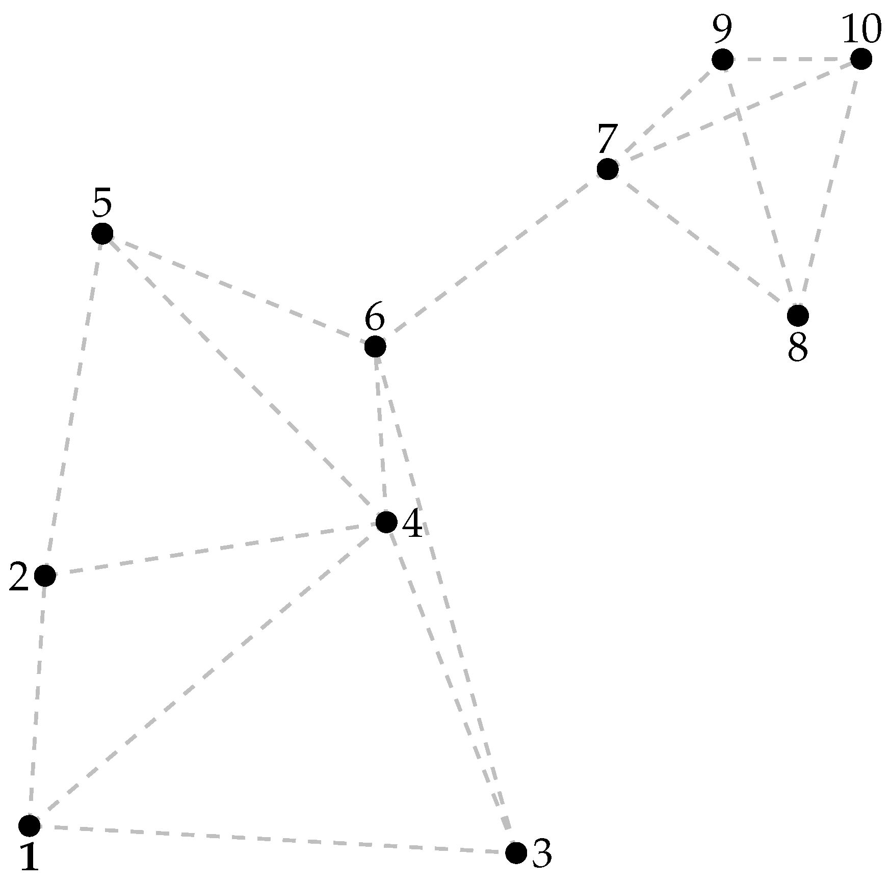
5.1. Results for the 10-Node Distribution System: Nuquí, Chocó

Table 11 and

Table 14. Selected routes and conductor calibers for the 10-node distribution system.

SSA		GWO		VSA		EO		MINLP		EO-MINLP
Line	Cal.	Line	Cal.	Line	Cal.	Line	Cal.	Line	Cal.	Line	Cal.
3	6	3	6	3	6	3	6	3	6	3	6
4	1	4	1	4	1	4	1	4	1	4	1
6	1	6	1	6	1	6	1	6	1	6	1
8	1	8	1	8	1	8	1	8	1	8	1
9	5	9	5	9	5	9	5	9	5	9	5
11	4	11	4	11	4	11	4	11	4	11	4
12	1	12	1	12	1	12	1	12	1	12	1
13	1	13	1	13	1	13	1	13	1	13	1
14	1	14	1	14	1	14	1	17	1	17	1

summarize the results obtained for the 10-node distribution system located in Nuquí, Chocó. The first table reports the route and conductor caliber selected by each solution strategy, whereas the second table presents the corresponding annual cost components, the standard deviation of the solution process, and the mean computational time.

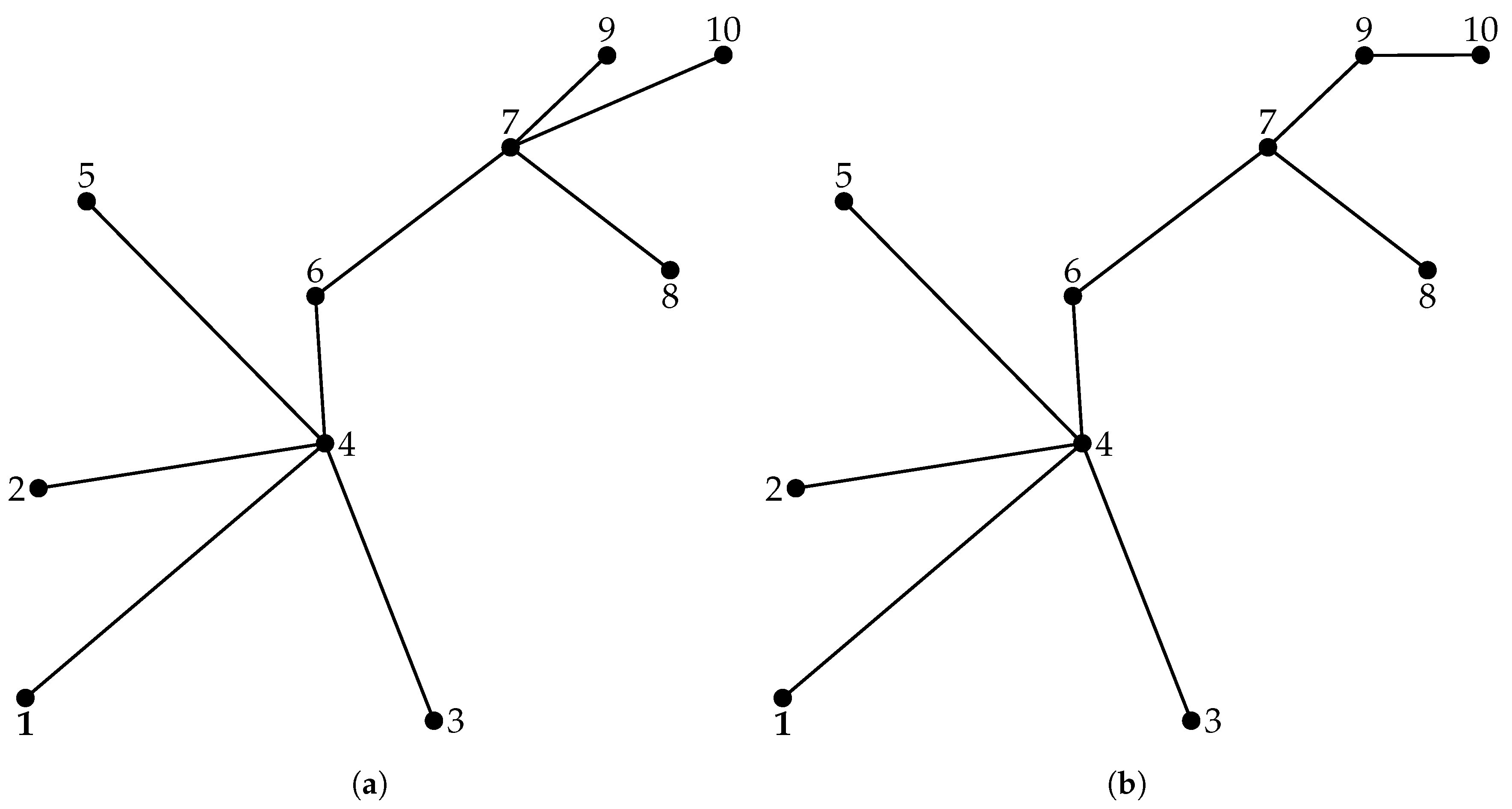
Table 14 shows that all metaheuristic approaches, namely, SSA, GWO, VSA, and EO, converged to the same radial topology and conductor allocation. In these solutions, the selected construction routes correspond to lines 3, 4, 6, 8, 9, 11, 12, 13, and 14, as illustrated in Figure 5a. The conductor calibers are also identical among the four metaheuristics, which indicates that, for this system, the search space contains a highly attractive feasible region that can be consistently identified by different population-based algorithms.

In contrast, the exact MINLP formulation and the proposed EO-MINLP strategy selected a slightly different topology. In both approaches, line 14 was replaced by line 17, as shown in Figure 5b, while the remaining selected routes and conductor sizes were preserved.

This modification is relevant because it demonstrates that a small topological change can improve the total annual cost, even when most of the network structure remains unchanged. Therefore, the difference between the metaheuristic solutions and the MINLP-based solutions is not associated with a generalized change in conductor sizing, but rather with a more effective selection of one route within the radial configuration. This result highlights the importance of solving route selection and conductor selection in an integrated manner, since the economic performance of the network is sensitive not only to conductor calibers but also to the spatial arrangement of the selected lines.

From the conductor selection perspective, the predominance of caliber 1 in the 10-node system is consistent with the rural nature of the network. Since the load density is low and the maximum conductor loading remains far below the thermal limit, the selected calibers are not mainly determined by ampacity requirements. Instead, the few branches assigned larger calibers, such as lines 3, 9, and 11, reveal that conductor sizing is driven by the need to control voltage drops and reduce the equivalent impedance of electrically relevant paths. Therefore, although most branches can be built with the smallest available caliber without violating current limits, the optimization model assigns larger conductors only where the feeder length, accumulated downstream demand, or voltage regulation requirements justify the additional investment.

Table 11 provides a more detailed economic comparison among the evaluated methods.

The metaheuristic methods SSA, GWO, VSA, and EO reached the same total annual cost of 49,353.4688 USD. This value is composed of 23,116.1636 USD associated with annual energy losses and 26,237.3052 USD associated with annualized conductor investment. The equality of these values confirms that all metaheuristics identified the same network configuration and conductor allocation.

The MINLP and EO-MINLP approaches achieved a lower total annual cost of 49,147.4576 USD, which represents a reduction of approximately 0.42% with respect to the metaheuristic-only solutions. Although this percentage may appear moderate, it is technically significant because the 10-node system is a small-scale network with a limited number of feasible radial configurations. In this context, even a small reduction in annual cost indicates that the exact–metaheuristic formulation was able to identify a more economically efficient trade-off between route construction and operational losses.

Regarding energy losses, the metaheuristic solutions obtained a lower annual loss cost, equal to 23,116.1636 USD, while the MINLP and EO-MINLP solutions obtained 23,462.3526 USD. This represents an increase of approximately 1.50% in annual losses for the MINLP-based solution. However, this increase is compensated by a reduction in the annualized investment cost. Specifically, the investment cost decreased from 26,237.3052 USD in the metaheuristic solutions to 25,685.1051 USD in the MINLP and EO-MINLP solutions, corresponding to a reduction of approximately 2.10%. Therefore, the best solution is not the one with the lowest technical losses, but the one that achieves the best economic balance between investment and operation.

This performance is explained by the fact that the hybrid method tends to incorporate a larger number of lateral branches (Figure 5), which reduces power concentration in the network sections and improves current distribution throughout the distribution system; as a result, Joule losses decrease. Additionally, by relieving the loading of the network sections, the solution assigns smaller conductor calibers to a larger portion of the network, thereby reducing the investment component without compromising compliance with the electrical constraints.

In terms of standard deviation, GWO, VSA, and EO exhibited values that were practically zero, in the order of ${10}^{-14}$, indicating that these algorithms consistently converged to the same solution. SSA also presented a low standard deviation of 0.14380%, showing stable behavior, although with slightly higher dispersion than the other metaheuristics. As expected, the MINLP solution presents zero standard deviation because it is obtained through a deterministic exact optimization process. The EO-MINLP strategy also reports zero standard deviation, confirming that the hybrid procedure was able to reproduce the exact MINLP solution for this test system.

The mean computational time shows that the pure metaheuristic approaches required between 63.9897 s and 81.2272 s, with VSA being the fastest method and SSA the slowest among them. The exact MINLP formulation required 113.0900 s, which is higher than the computational time of the metaheuristics. This behavior is expected, since the MINLP model performs a more rigorous exploration of the feasible space and explicitly handles the nonlinear electrical constraints and discrete conductor decisions. The proposed EO-MINLP strategy required 95.2335 s, reducing the computational time by approximately 15.79% compared with the standalone MINLP formulation, while preserving the same optimal objective value. This result indicates that the hybrid strategy can improve computational efficiency without sacrificing solution quality.

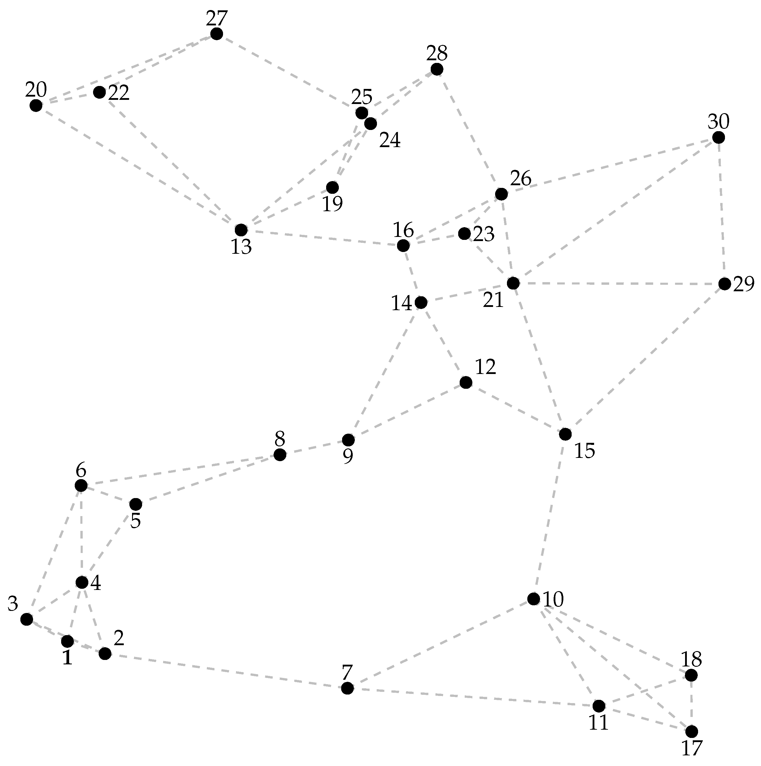
5.2. Results for the 30-Node Distribution System: Leticia, Amazonas

Table 12 and

Table 15. Selected routes and conductor calibers for the 30-node distribution system.

SSA		GWO		VSA		EO		MINLP		EO-MINLP
Line	Cal.	Line	Cal.	Line	Cal.	Line	Cal.	Line	Cal.	Line	Cal.
1	6	1	6	1	6	1	6	1	6	1	6
4	5	4	4	4	4	4	4	4	4	4	4
5	6	5	6	5	6	5	6	5	6	5	6
6	6	6	6	6	6	6	6	6	6	6	6
8	4	8	3	8	4	8	4	8	4	8	4
9	6	9	6	9	6	9	6	9	6	9	6
12	6	12	6	12	6	12	6	12	6	12	6
14	6	14	6	14	6	14	6	14	6	14	6
15	6	15	5	15	6	15	6	15	5	15	6
16	6	16	6	16	6	16	6	16	6	16	6
17	4	18	6	17	3	17	4	17	3	17	3
18	6	20	6	18	6	18	6	18	6	18	6
20	6	22	1	20	6	20	6	20	6	20	6
23	4	23	4	23	4	23	4	22	1	23	4
24	1	26	3	27	6	24	1	23	4	24	1
27	6	27	6	29	4	27	6	27	6	27	6
28	4	28	5	30	4	29	4	28	5	28	5
29	4	30	6	31	4	30	2	30	6	30	6
30	4	32	6	32	6	31	4	32	6	32	6
31	4	34	6	34	6	32	6	34	6	34	6
32	6	35	4	35	4	34	6	35	4	35	4
34	6	36	4	36	4	35	4	36	4	39	4
35	4	40	3	38	1	36	4	40	4	41	4
36	3	41	5	40	4	40	4	41	3	42	4
42	4	42	4	42	4	42	4	44	5	43	4
44	5	44	5	44	6	44	6	47	4	44	5
52	4	46	2	46	2	52	5	50	4	52	4
53	5	50	4	52	5	53	5	53	5	53	5
55	3	53	5	53	5	55	2	55	2	55	2

summarize the results obtained for the 30-node distribution system located in Leticia, Amazonas. These tables contain the same type of information as the tables presented for the 10-node system.

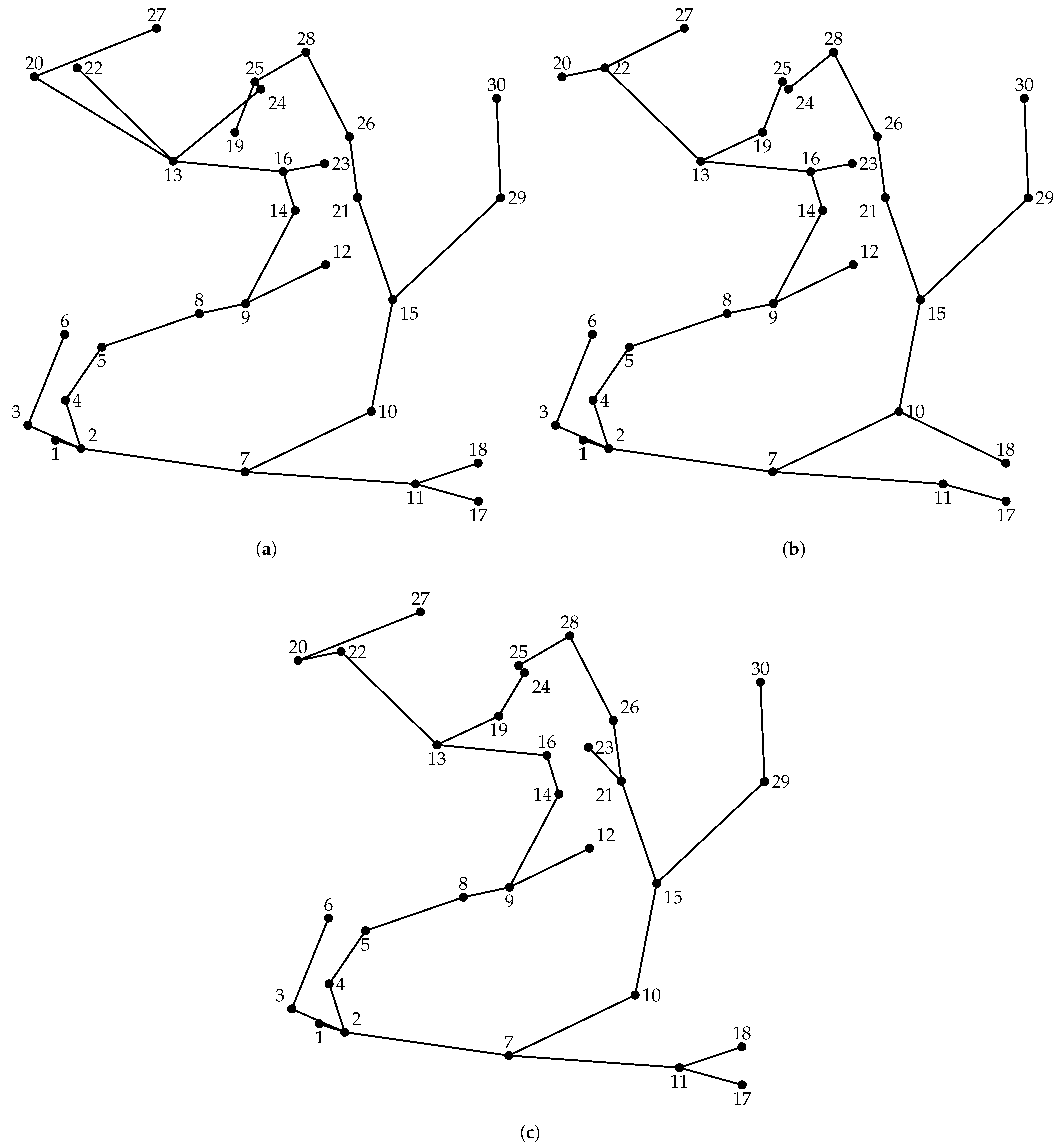
Table 15 presents the selected routes and conductor sizes obtained with SSA, GWO, VSA, EO, MINLP, and EO-MINLP, where it can be observed that the specific set of selected lines varies across the methodologies, indicating that the larger search space leads to different feasible radial topologies. This contrasts with the 10-node case, where most methods converged to nearly the same configuration.

Figure 6 complements the information reported in Table 15 by visually comparing the radial topologies obtained for the 30-node system.

As observed in Figure 6, the best metaheuristic solution, the exact MINLP solution, and the hybrid solution share a common structural backbone composed mainly of lines 1, 4, 5, 6, 8, 9, 12, 14, 15, 16, 17, 18, 20, 23, 27, 30, 32, 34, 35, 44, 53, and 55. These routes preserve the main feeder paths and guarantee radial connectivity, suggesting that they are structurally relevant corridors for the 30-node system. However, the differences observed in the remaining branches confirm that the system admits multiple feasible radial alternatives. In particular, the variations in the upper and terminal sections of the feeder show that small changes in route selection can modify the way power flows are distributed through the network. Therefore, compared with the 10-node case, the route selection stage becomes more sensitive to the search strategy, since different algorithms may identify alternative radial configurations with similar feasibility but different economic and operational performance.

Regarding conductor selection, calibers 6, 5, and 4 are mainly assigned to the most relevant or highly loaded sections of the network, particularly in branches close to the substation or in paths that supply a larger portion of the feeder. In contrast, calibers 1, 2, and 3 appear in more specific terminal or lightly loaded branches, where current flow and voltage-drop impact are less critical. This behavior is consistent with the semi-urban nature of the 30-node system: unlike the rural 10-node case, where conductor sizing is mainly governed by voltage regulation under low loading conditions, the Leticia system requires a more balanced planning criterion. In this case, conductor selection must simultaneously account for current-carrying capacity, voltage regulation, and investment cost, since higher loading levels near the substation and more severe voltage drops at the feeder ends make both technical and economic effects relevant in the final solution.

The comparison between MINLP and EO-MINLP shows that both approaches identify different radial topologies. This indicates that the hybrid strategy does not simply reproduce the standalone MINLP solution; instead, it guides the search toward an alternative feasible configuration with better economic performance by combining the exploration capacity of EO with the rigorous conductor evaluation of the MINLP model.

From Table 12, it can be seen that EO-MINLP obtained the lowest total annual cost, with 436,610.1270 USD. The standalone MINLP formulation reached 437,251.4735 USD, while the best pure metaheuristic solution was obtained by EO, with 439,716.6985 USD. Therefore, EO-MINLP reduced the total annual cost by 641.3465 USD, equivalent to approximately 0.15%, with respect to the standalone MINLP. Similarly, when compared with the best pure metaheuristic, EO-MINLP achieved an annual saving of 3106.5715 USD, corresponding to approximately 0.71%. Although these differences may seem moderate in percentage terms, they are relevant in planning problems because the objective function represents an annualized cost. Consequently, even small annual savings may accumulate significantly over the planning horizon.

Moreover, EO-MINLP achieved the lowest annual loss cost, equal to 348,383.8475 USD. This value is lower than the loss cost obtained by the standalone MINLP, which was 352,416.9334 USD, and also lower than the best metaheuristic loss cost, obtained by SSA with 351,376.4414 USD. In particular, EO-MINLP reduced the loss cost by approximately 1.14% with respect to MINLP and by approximately 0.85% with respect to the best metaheuristic value. This result shows that the topology selected by EO-MINLP is not only economically competitive but also electrically more efficient in terms of active power losses.

Regarding the annualized investment cost, the standalone MINLP obtained the lowest value, equal to 84,834.5400 USD. This means that the exact formulation identified a less expensive infrastructure configuration in terms of conductor investment. However, this lower investment cost was accompanied by a higher annual loss cost. On the other hand, EO-MINLP obtained an investment cost of 88,226.2795 USD, which is higher than the MINLP investment cost but lower than or comparable to several metaheuristic solutions. This confirms that EO-MINLP selected a slightly more expensive infrastructure, but one that produced a greater reduction in losses. As a result, the hybrid solution achieved the lowest total annual cost.

On the other hand, the pure metaheuristic methods presented standard deviations ranging from 1.0769% to 1.7084%, which are higher than those obtained for the 10-node system. This behavior is expected, since the 30-node system involves a larger combinatorial search space, making it more difficult for the algorithms to consistently converge to the same solution over multiple runs. Among the pure metaheuristics, VSA achieved the lowest standard deviation, with 1.0769%, followed by GWO, EO, and SSA. As expected, the standalone MINLP formulation reported zero standard deviation due to its deterministic nature. In contrast, EO-MINLP achieved a low standard deviation of 0.1099%, indicating that the hybrid strategy significantly improves the repeatability of the stochastic search while maintaining a high-quality solution.

Finally, the computational time highlights the main computational challenge of the exact optimization approach. The pure metaheuristics required between 217.7099 s and 295.9033 s, with EO being the fastest method. In contrast, the standalone MINLP formulation required 39,562.0100 s, which reflects the computational burden associated with solving the nonlinear and discrete optimization problem exactly for a larger network. The EO-MINLP strategy required 8433.3063 s, which is considerably higher than the pure metaheuristics but much lower than the standalone MINLP. Specifically, EO-MINLP reduced the computational time by approximately 78.68% with respect to MINLP, while also improving the final objective value. This result demonstrates the practical advantage of the hybrid strategy for larger systems.

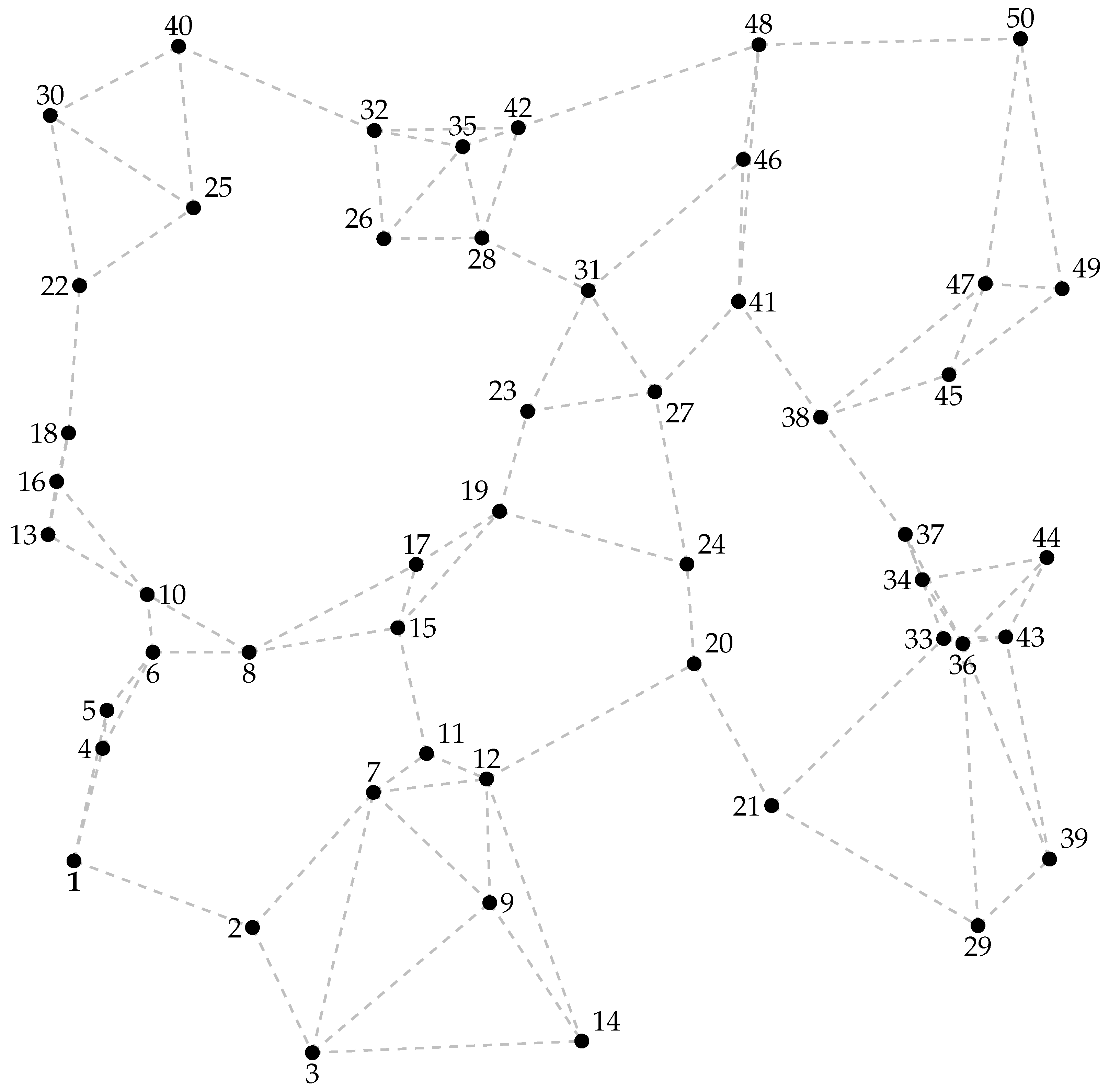
5.3. Results for the 50-Node Distribution System: San Andres Island

Table 13 and

Table 16. Selected routes and conductor calibers for the 50-node distribution system.

SSA		GWO		VSA		EO		MINLP		EO-MINLP
Line	Cal.	Line	Cal.	Line	Cal.	Line	Cal.	Line	Cal.	Line	Cal.
2	6	2	6	2	6	2	6	2	6	2	6
4	5	5	2	5	5	4	4	5	3	4	5
5	5	6	4	6	5	5	6	6	5	5	6
9	5	9	4	9	5	9	3	9	5	9	5
10	6	10	6	10	6	10	6	10	6	10	6
12	6	12	6	12	6	12	6	12	6	12	6
13	6	13	6	13	6	13	6	13	6	13	6
15	6	15	3	14	6	15	6	14	6	14	6
18	6	18	6	15	6	18	6	15	6	15	6
19	6	19	6	18	6	19	6	18	6	18	6
20	6	20	4	19	6	20	6	19	6	19	6
21	3	22	6	21	3	21	4	21	4	21	3
22	6	23	5	22	6	22	6	22	6	22	6
23	6	24	6	23	5	23	5	23	5	23	5
24	6	25	6	24	6	24	6	24	6	24	6
25	6	26	3	25	6	25	6	25	6	25	6
27	6	27	6	27	6	27	6	27	6	27	6
29	6	29	6	29	6	29	6	29	6	29	6
33	6	33	6	33	6	33	6	33	6	33	6
34	6	34	6	34	6	34	6	34	6	34	6
35	6	35	6	35	6	35	6	35	6	35	6
36	4	36	6	36	4	36	3	36	4	36	4
37	6	37	6	37	6	37	6	37	6	37	6
39	4	39	3	39	6	39	6	39	5	39	4
40	6	40	6	40	6	40	6	40	6	40	6
41	6	41	6	41	4	41	6	41	4	41	6
42	4	44	6	42	6	43	6	42	6	42	4
43	6	45	6	43	6	44	6	43	6	43	6
44	4	46	3	44	6	46	4	44	6	44	6
47	6	47	6	48	5	47	6	48	5	47	6
48	5	49	6	49	6	49	5	49	6	49	5
49	6	50	5	52	5	52	6	52	6	52	6
52	6	52	6	56	1	54	4	56	4	54	5
57	2	53	5	57	5	56	5	57	3	57	3
60	6	57	4	58	6	57	3	58	6	59	5
61	6	59	3	59	6	59	5	59	4	60	6
63	3	61	6	60	5	60	6	60	4	61	6
66	2	63	3	61	4	61	6	61	6	64	5
69	2	66	3	62	4	63	3	62	5	66	4
70	6	70	2	63	5	65	4	63	5	67	5
71	4	74	3	65	1	69	2	65	2	69	1
75	5	75	4	66	6	70	2	66	4	70	2
76	6	76	6	69	6	73	4	69	1	75	4
77	6	77	5	76	4	76	6	76	6	76	6
78	4	78	4	77	3	77	2	77	4	77	6
82	6	81	3	78	6	78	5	78	6	84	4
85	5	83	4	82	5	82	3	82	5	85	5
86	5	85	4	87	5	87	3	87	4	86	4
89	1	88	1	89	1	90	3	89	1	90	1

present the results obtained for the 50-node distribution system. Compared with the 10- and 30-node cases, this system represents a more challenging planning scenario due to the larger number of candidate routes, radial configurations, and conductor assignment possibilities. Consequently, the differences among the evaluated methods become more evident, especially in the selected topology and in the balance between investment and energy losses.

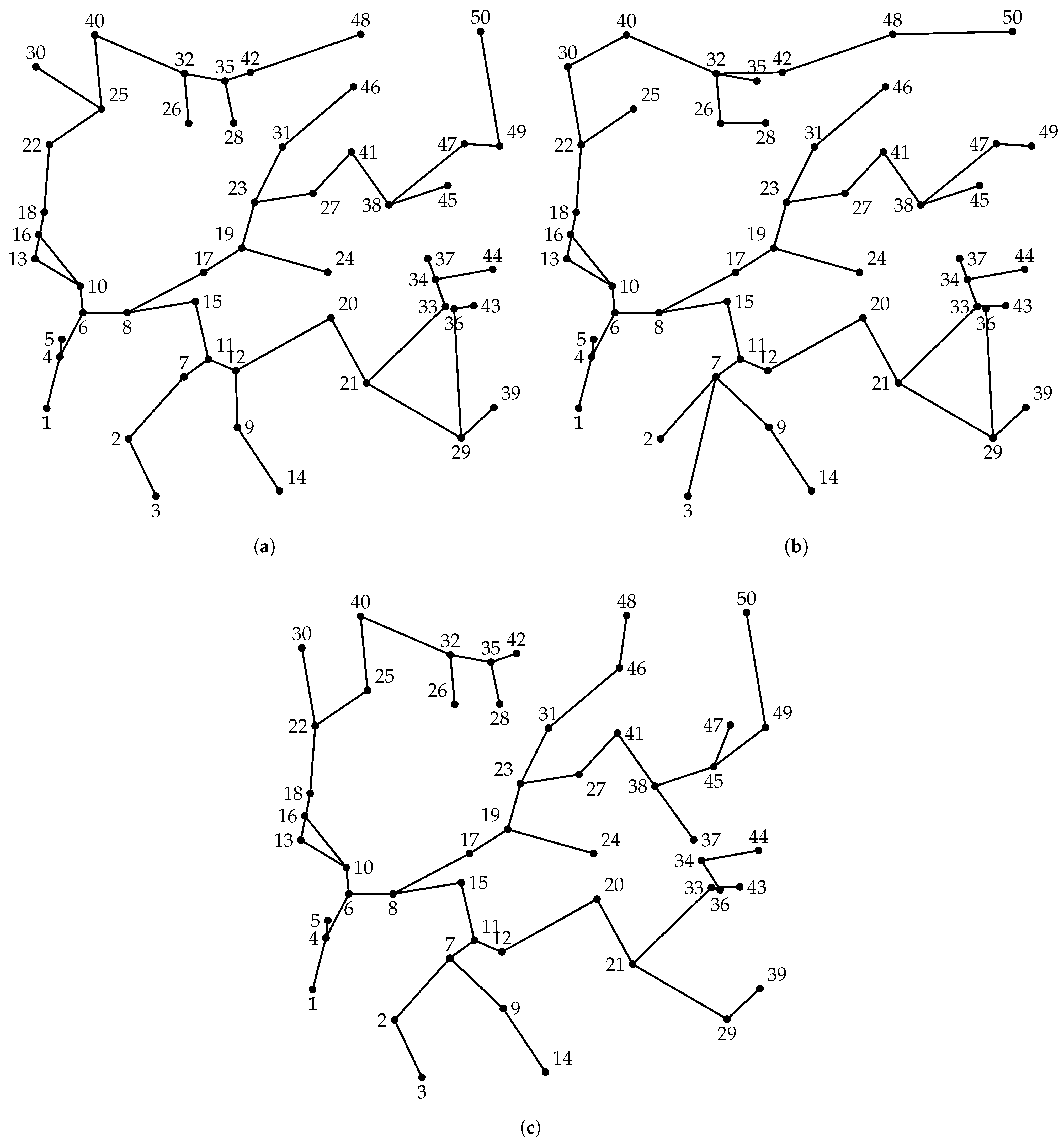
Figure 7 complements the information reported in Table 16 by comparing the radial topologies obtained for the 50-node system.

Unlike the smaller systems, the selected routes exhibit a higher degree of diversity among the methodologies. Although the best metaheuristic solution, the exact MINLP solution, and the hybrid solution preserve a common structural backbone in several parts of the network, important differences appear in the lateral and terminal branches. This behavior is particularly evident in the upper-left, central, and right-side sections of the feeder, where the algorithms select different connections to preserve radiality and satisfy the electrical constraints.

This higher topological diversity confirms that, as the system size increases, the route selection problem becomes more sensitive to the exploration strategy used by each algorithm. In the 50-node case, small changes in the selected routes can significantly modify the distribution of power flows, voltage drops, and losses throughout the feeder. Therefore, the differences observed in Figure 7 explain why the evaluated methods lead to different investment and loss components, even when all solutions satisfy the radiality condition. In this context, the hybrid EO-MINLP strategy is able to exploit alternative radial configurations more effectively, leading to the best economic performance reported in Table 13.

From the conductor selection perspective, calibers 6 and 5 are frequently assigned to the main sections of the network, while calibers 1, 2, 3, and 4 are used in more specific lateral or terminal branches. This behavior is consistent with the urban characteristics of the 50-node system, where the higher demand density produces larger current peaks near the substation and in the main feeder sections. Unlike the rural 10-node case, where conductor loading was not critical, in this system the loading level reaches values close to the thermal limit, making ampacity an active design condition. Therefore, larger calibers are required not only to reduce voltage drops but also to ensure adequate current-carrying capacity in the most stressed branches. At the same time, smaller calibers are assigned to less loaded sections to avoid unnecessary investment.

The comparison between MINLP and EO-MINLP is especially relevant for this case. Both approaches select different topologies and conductor allocations. EO-MINLP guides the search toward an alternative radial configuration with better economic performance. This behavior becomes more significant in the 50-node system, where the exact MINLP formulation faces a much larger combinatorial space and, consequently, a higher computational burden. Thus, the hybridization allows the exploration capacity of EO to be combined with the rigorous conductor evaluation of the MINLP model.

From Table 13, it can be observed that EO-MINLP obtained the lowest total annual cost, with 1,069,605.0150 USD. The standalone MINLP formulation reached 1,078,691.2328 USD, while the best pure metaheuristic solution was obtained by EO, with 1,084,334.6538 USD. Therefore, EO-MINLP reduced the total annual cost by 9086.2178 USD, equivalent to approximately 0.84%, with respect to the standalone MINLP. Similarly, when compared with the best pure metaheuristic, EO-MINLP achieved an annual saving of 14,729.6388 USD, corresponding to approximately 1.36%. These savings are more pronounced than those observed in the smaller test systems, showing that the benefits of the hybrid strategy become more relevant as the network size increases.

The annual loss cost is the dominant component of the objective function in this system. For all methods, this component represents most of the total annual cost, which indicates that the operational efficiency of the selected topology has a strong impact on the final planning decision. EO-MINLP obtained the lowest annual loss cost, with 986,210.1854 USD. This value represents a reduction of 4523.4210 USD, or approximately 0.46%, with respect to the standalone MINLP. Compared with the best pure metaheuristic in terms of total annual cost, EO, the loss reduction achieved by EO-MINLP was 11,247.7651 USD, equivalent to approximately 1.13%. This result shows that the hybrid strategy identified a topology and conductor allocation that improved the operational behavior of the network.

Regarding the annualized investment cost, EO-MINLP also achieved a competitive result, with 83,394.8296 USD. This value is lower than the investment cost obtained by SSA, VSA, EO, and MINLP. In particular, EO-MINLP reduced the investment cost by 4562.7969 USD, equivalent to approximately 5.19%, with respect to the standalone MINLP. Although GWO obtained the lowest investment cost, with 82,555.5830 USD, this solution presented the highest loss cost and the highest total annual cost among all methods. Therefore, the lowest investment cost does not necessarily lead to the best planning solution. In this case, EO-MINLP achieved the best global balance by simultaneously reducing losses and maintaining a low investment cost.

The standard deviation values confirm the increasing complexity of the 50-node system. The pure metaheuristics presented standard deviations between $0.4542\%$ and $1.1356\%$. VSA achieved the lowest dispersion among the pure metaheuristic methods, followed by EO, GWO, and SSA. The standalone MINLP formulation reported zero standard deviation due to its deterministic nature. EO-MINLP presented a standard deviation of $0.3768\%$, which is lower than that of all pure metaheuristics. This indicates that the hybrid strategy improves the repeatability of the stochastic search while maintaining the best objective value among all evaluated methods.

The computational time highlights the main limitation of the standalone MINLP approach for larger systems. The pure metaheuristics required between 516.5858 s and 639.3958 s, with EO being the fastest method. In contrast, the standalone MINLP formulation required 535,680.0000 s, evidencing the high computational burden associated with the exact solution of the 50-node route and conductor selection problem. EO-MINLP required 59,218.2661 s, which is considerably higher than the pure metaheuristics but much lower than the standalone MINLP. Specifically, EO-MINLP reduced the computational time by 476,461.7339 s, equivalent to approximately 88.95%, with respect to MINLP. This reduction is substantial and confirms the computational advantage of the hybrid strategy for larger-scale planning problems.

Overall, the results obtained for the 10-, 30-, and 50-node test systems demonstrate that the optimal planning criterion in unbalanced three-phase distribution networks strongly depends on the operating context and the network scale. In the rural 10-node system, the presence of long feeders and low current levels makes voltage regulation and the electrical efficiency of the selected paths more relevant than thermal loading limits. In the semi-urban 30-node system, a mixed behavior is observed: higher demand levels increase the relevance of current flow and make the investment–loss trade-off more sensitive to the selected topology and conductor sizes. Finally, in the urban 50-node system, the greater load density causes power losses to dominate the annualized cost, making it essential to coordinate route selection and conductor sizing to improve the operational efficiency of the network.

These results also confirm the scalability of the proposed EO-MINLP methodology. As the number of nodes increases, the combinatorial complexity of the route selection problem grows significantly, making the standalone MINLP formulation computationally demanding. However, the hybrid strategy consistently obtained the best total annual cost in the 30- and 50-node systems and reproduced the exact MINLP solution in the 10-node system, while reducing computational effort with respect to the standalone exact approach. Therefore, the proposed methodology provides a suitable balance between solution quality, repeatability, and computational tractability, showing its potential for solving larger and more realistic distribution network planning problems.

5.4. Large-Scale Validation and Scalability-Oriented Extensions

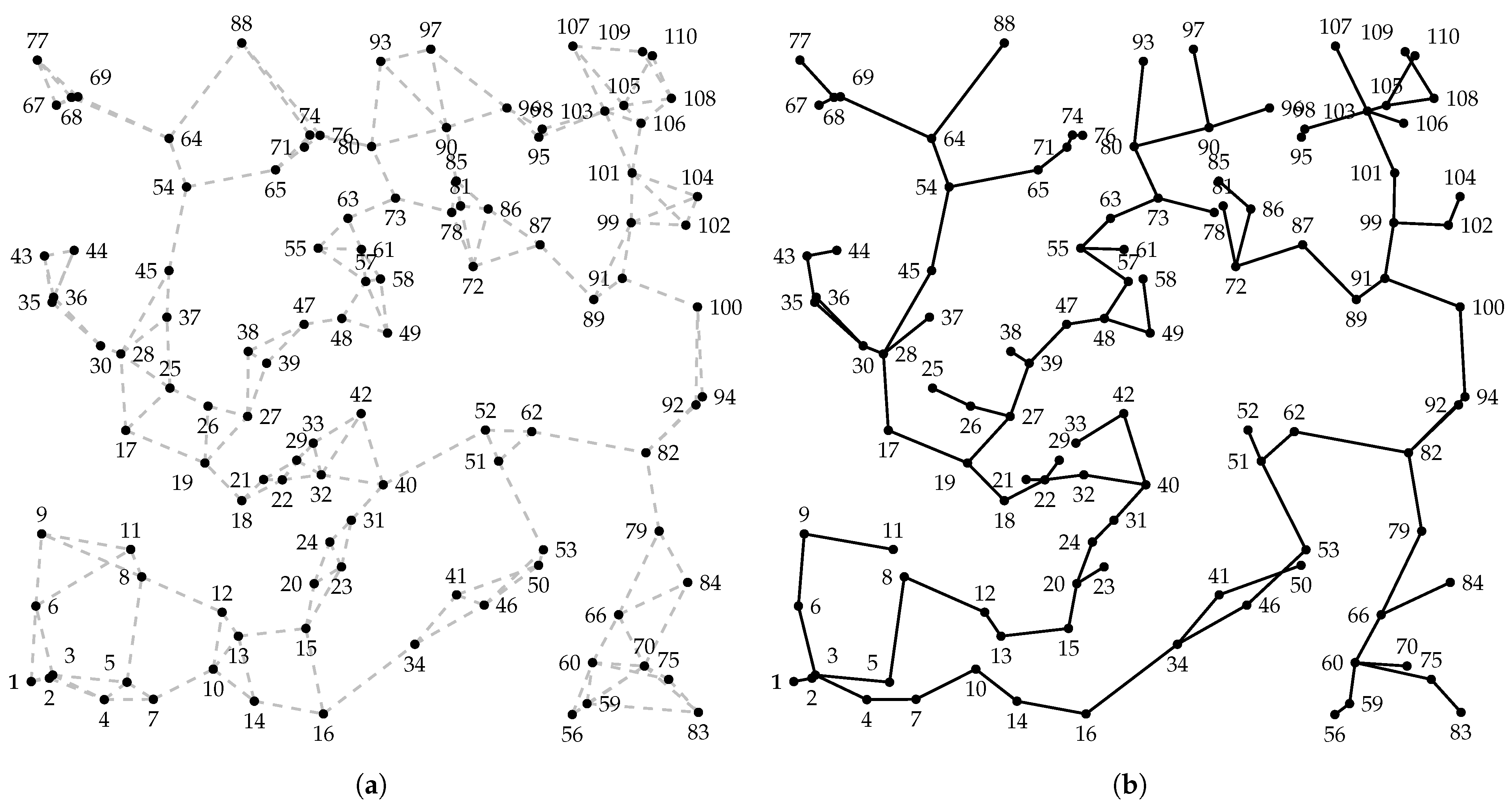
To further assess the computational scalability of the proposed methodology, an additional urban distribution network with 110 nodes was considered. The system is supplied at 13.2 kV line-to-line from the substation located at node 1 and comprises 109 load buses, with a maximum of 50 users per node and an average population density of 1100 users/km². The total active and reactive power demands are 2602.7 kW and 657.9 kvar for phase A, 2232.1 kW and 569.5 kvar for phase B, and 2709.8 kW and 702.1 kvar for phase C, respectively. The route-planning stage includes 197 candidate line sections, which substantially increases the combinatorial search space compared with the 10-, 30-, and 50-node systems. The complete set of candidate routes is illustrated in Figure 8a.

Table A1. Nodal three-phase load demand profile for the 110-node distribution system.

Node i	${\mathit{P}}_{\mathit{iA}}$	${\mathit{Q}}_{\mathit{iA}}$	${\mathit{P}}_{\mathit{iB}}$	${\mathit{Q}}_{\mathit{iB}}$	${\mathit{P}}_{\mathit{iC}}$	${\mathit{Q}}_{\mathit{iC}}$	Type
1	0	0	0	0	0	0	$\Delta$
2	6	2	0	0	46	12	$\Delta$
3	0	0	0	0	14	4	Y
4	0	0	18	5	6	2	$\Delta$
5	0	0	3	1	7	2	Y
6	20	5	0	0	0	0	$\Delta$
7	0	0	12	3	0	0	Y
8	47	12	36	9	20	5	Y
9	0	0	12	3	2	1	Y
10	0	0	0	0	39	10	$\Delta$
11	3	1	50	13	28	7	Y
12	23	6	0	0	0	0	Y
13	36	9	0	0	3	1	$\Delta$
14	17	4	0	0	33	8	Y
15	38	10	26	7	7	2	$\Delta$
16	3	1	0	0	28	7	Y
17	25	6	15	4	0	0	Y
18	37	9	0	0	0	0	Y
19	8	2	0	0	0	0	$\Delta$
20	1	0	0	0	0	0	$\Delta$
21	0	0	29	7	45	11	$\Delta$
22	32	8	0	0	43	11	Y
23	13	3	0	0	0	0	Y
24	14	4	24	6	15	4	Y
25	4	1	0	0	42	11	Y
26	9	2	24	6	0	0	$\Delta$
27	41	10	0	0	38	10	$\Delta$
28	21	5	0	0	0	0	Y
29	16	4	0	0	0	0	Y
30	0	0	0	0	5	1	Y
31	3	1	0	0	0	0	Y
32	0	0	0	0	34	9	$\Delta$
33	0	0	47	12	38	10	$\Delta$
34	5	1	30	8	0	0	Y
35	0	0	14	4	0	0	Y
36	12	3	0	0	13	3	$\Delta$
37	32	8	0	0	32	8	$\Delta$
38	21	5	45	11	0	0	Y
39	18	5	0	0	10	3	$\Delta$
40	0	0	36	9	28	7	$\Delta$
41	24	6	0	0	0	0	Y
42	0	0	15	4	0	0	Y
43	46	12	0	0	0	0	$\Delta$
44	48	12	44	11	3	1	$\Delta$
45	8	2	0	0	0	0	Y
46	29	7	0	0	0	0	$\Delta$
47	40	10	10	3	0	0	Y
48	0	0	35	9	18	5	$\Delta$
49	11	3	0	0	11	3	$\Delta$
50	23	6	0	0	0	0	$\Delta$
51	22	6	0	0	0	0	$\Delta$
52	45	11	7	2	43	11	$\Delta$
53	26	7	0	0	0	0	$\Delta$
54	10	3	7	2	47	12	$\Delta$
55	0	0	49	12	16	4	Y
56	20	5	29	7	30	8	$\Delta$
57	5	1	39	10	32	8	$\Delta$
58	45	11	0	0	42	11	Y
59	0	0	45	11	0	0	Y
60	16	4	47	12	23	6	$\Delta$
61	0	0	0	0	8	2	Y
62	17	4	22	6	30	8	Y
63	0	0	14	4	0	0	$\Delta$
64	0	0	20	5	0	0	$\Delta$
65	0	0	0	0	7	2	Y
66	0	0	12	3	14	4	$\Delta$
67	25	6	47	12	0	0	$\Delta$
68	23	6	14	4	0	0	$\Delta$
69	0	0	0	0	26	7	$\Delta$
70	14	4	0	0	12	3	Y
71	0	0	48	12	11	3	Y
72	22	6	0	0	15	4	Y
73	0	0	0	0	41	10	$\Delta$
74	0	0	0	0	18	5	$\Delta$
75	0	0	0	0	16	4	Y
76	0	0	13	3	0	0	Y
77	4	1	44	11	0	0	Y
78	0	0	0	0	36	9	Y
79	0	0	11	3	0	0	Y
80	24	6	36	9	7	2	Y
81	33	8	0	0	0	0	$\Delta$
82	35	9	0	0	3	1	$\Delta$
83	35	9	0	0	0	0	$\Delta$
84	0	0	0	0	2	1	$\Delta$
85	0	0	23	6	40	10	Y
86	35	9	29	7	10	3	$\Delta$
87	0	0	24	6	36	9	Y
88	4	1	0	0	42	11	$\Delta$
89	33	8	30	8	22	6	$\Delta$
90	0	0	7	2	0	0	$\Delta$
91	0	0	40	10	0	0	$\Delta$
92	24	6	0	0	1	0	$\Delta$
93	17	4	2	1	43	11	Y
94	0	0	17	4	0	0	Y
95	26	7	4	1	0	0	$\Delta$
96	6	2	0	0	0	0	Y
97	29	7	5	1	26	7	$\Delta$
98	36	9	0	0	0	0	Y
99	15	4	16	4	47	12	Y
100	0	0	0	0	46	12	Y
101	0	0	4	1	36	9	$\Delta$
102	39	10	0	0	0	0	$\Delta$
103	0	0	7	2	29	7	Y
104	2	1	3	1	0	0	$\Delta$
105	0	0	36	9	0	0	Y
106	24	6	0	0	27	7	$\Delta$
107	0	0	4	1	42	11	$\Delta$
108	0	0	16	4	31	8	Y
109	41	10	17	4	29	7	$\Delta$
110	45	11	0	0	0	0	Y

and

Table A2. Candidate distribution routes in the 110-node system.

Line (Connection)	Length (m)	Line (Connection)	Length (m)
1 (1–2)	60.0167	100 (55–63)	136.4734
2 (1–3)	73.0821	101 (56–59)	59.4054
3 (1–6)	243.4625	102 (56–60)	179.5689
4 (2–3)	14.8661	103 (56–70)	282.0656
5 (2–4)	191.8385	104 (57–58)	48.6621
6 (3–4)	185.6475	105 (57–61)	103.9471
7 (3–5)	243.0905	106 (58–61)	113.4416
8 (3–6)	228.7116	107 (59–60)	133.2216
9 (4–5)	92.8009	108 (59–70)	222.7330
10 (4–7)	160.0031	109 (59–83)	364.0783
11 (5–7)	102.0833	110 (60–66)	175.9005
12 (5–8)	342.3814	111 (60–70)	169.3576
13 (6–9)	232.7767	112 (60–75)	253.8110
14 (6–11)	358.6154	113 (61–63)	109.2520
15 (7–10)	217.7935	114 (62–82)	378.1640
16 (8–9)	354.0056	115 (63–73)	168.0774
17 (8–11)	95.0789	116 (64–68)	344.3080
18 (8–12)	285.7271	117 (64–69)	325.8297
19 (9–11)	294.2788	118 (64–88)	387.8376
20 (10–12)	185.2836	119 (65–71)	119.0168
21 (10–13)	134.0149	120 (65–74)	158.3919
22 (10–14)	169.0118	121 (66–70)	185.1513
23 (12–13)	93.4773	122 (66–79)	299.6415
24 (13–14)	215.3718	123 (66–84)	247.8730
25 (13–15)	221.4159	124 (67–68)	55.0091
26 (14–16)	228.7051	125 (67–69)	75.0267
27 (15–16)	280.8452	126 (67–77)	157.6991
28 (15–20)	146.5094	127 (68–69)	21.0950
29 (15–23)	229.4777	128 (68–77)	163.4656
30 (16–34)	372.8002	129 (69–77)	177.0537
31 (17–19)	278.5480	130 (70–75)	89.9444
32 (17–25)	198.0707	131 (70–83)	230.6014
33 (17–28)	246.5198	132 (70–84)	303.7137
34 (18–19)	170.4142	133 (71–74)	42.9535
35 (18–21)	98.3107	134 (71–76)	63.6003
36 (18–22)	148.0304	135 (72–78)	187.5527
37 (19–26)	183.2730	136 (72–81)	199.2636
38 (19–27)	204.5018	137 (72–86)	191.3792
39 (20–23)	104.1009	138 (72–87)	228.9629
40 (20–24)	143.3771	139 (73–78)	188.6929
41 (21–22)	61.0082	140 (73–80)	183.4121
42 (21–29)	124.5311	141 (74–76)	33.0151
43 (22–29)	78.6003	142 (74–80)	204.3771
44 (22–32)	128.0039	143 (74–88)	370.0000
45 (22–33)	155.3222	144 (75–83)	143.6837
46 (23–24)	88.5664	145 (76–80)	171.8139
47 (23–31)	153.3754	146 (76–88)	391.4511
48 (24–31)	98.9949	147 (78–81)	35.8050
49 (25–26)	136.8941	148 (78–85)	102.1078
50 (25–28)	194.1649	149 (79–82)	255.6423
51 (25–37)	228.2192	150 (79–84)	189.4043
52 (26–27)	133.1540	151 (80–90)	251.5094
53 (27–38)	209.0096	152 (80–93)	275.6374
54 (27–39)	181.8928	153 (81–85)	81.2158
55 (28–30)	70.9366	154 (81–86)	90.5539
56 (28–37)	190.8507	155 (82–92)	224.2432
57 (28–45)	310.6010	156 (82–94)	257.4024
58 (29–32)	92.7847	157 (85–86)	137.5354
59 (29–33)	77.0779	158 (85–90)	174.9514
60 (30–35)	211.1019	159 (86–87)	204.4162
61 (30–36)	218.5063	160 (87–89)	248.1955
62 (31–40)	154.3114	161 (89–91)	115.2085
63 (32–33)	105.2616	162 (89–99)	275.4868
64 (32–40)	204.5189	163 (90–93)	301.9354
65 (32–42)	236.0275	164 (90–96)	206.8284
66 (33–42)	182.6499	165 (90–97)	257.1089
67 (34–41)	209.2295	166 (91–99)	181.3339
68 (34–46)	258.7508	167 (91–100)	261.7040
69 (35–36)	16.7631	168 (92–94)	33.4215
70 (35–43)	151.0828	169 (92–100)	315.0400
71 (35–44)	181.8598	170 (93–97)	167.6007
72 (36–43)	136.3415	171 (94–100)	289.4400
73 (36–44)	165.1969	172 (95–96)	140.1856
74 (37–45)	150.1632	173 (95–98)	28.2312
75 (38–39)	71.0211	174 (95–103)	230.8300
76 (38–47)	201.7251	175 (96–97)	311.8092
77 (39–47)	174.6683	176 (96–98)	133.6001
78 (40–42)	240.0521	177 (98–103)	212.0800
79 (40–52)	376.6497	178 (99–101)	160.0300
80 (41–46)	95.8593	179 (99–102)	178.1800
81 (41–50)	283.3972	180 (99–104)	231.7600
82 (43–44)	98.6560	181 (101–102)	242.5900
83 (45–54)	274.9727	182 (101–103)	218.0000
84 (46–50)	218.4331	183 (101–104)	226.1500
85 (46–53)	262.5509	184 (101–106)	162.6100
86 (47–48)	124.4588	185 (102–104)	99.5389
87 (48–49)	156.2370	186 (103–105)	64.5600
88 (48–57)	142.2849	187 (103–106)	124.2800
89 (49–57)	180.5464	188 (103–107)	233.4500
90 (49–58)	175.5135	189 (105–106)	79.9062
91 (50–53)	52.4976	190 (105–107)	253.0600
92 (51–52)	108.8531	191 (105–108)	156.7000
93 (51–53)	320.2202	192 (105–110)	185.0600
94 (51–62)	143.8367	193 (106–108)	127.2800
95 (52–62)	151.0828	194 (107–109)	227.7100
96 (54–64)	166.0873	195 (108–109)	177.0200
97 (54–65)	295.1694	196 (108–110)	150.3800
98 (55–57)	188.3454	197 (109–110)	34.5398
99 (55–61)	141.0567

summarize the main parameters of the 110-node test system, including the nodal load data and the candidate line sections considered for network construction.

Table 17. Selected routes and conductor sections for the 110-node distribution system using the EO-MINLP methodology.

Line	Cal.	Line	Cal.	Line	Cal.	Line	Cal.	Line	Cal.
1	6	43	2	87	2	128	2	179	2
4	6	44	6	88	6	133	1	182	6
6	6	48	6	90	6	136	1	185	5
7	6	49	1	92	2	137	3	186	6
8	6	52	6	93	6	138	6	187	3
10	6	54	6	94	6	139	1	188	2
12	6	55	4	96	1	140	6	191	6
13	6	56	1	97	3	141	4	192	1
15	6	57	6	98	5	144	4	195	6
18	6	60	2	99	1	149	6
19	6	61	1	100	4	151	1
22	6	62	6	101	1	152	5
23	6	64	6	107	4	155	2
25	6	66	6	110	6	156	6
26	6	67	2	111	1	157	2
28	6	68	6	112	1	160	2
30	6	70	2	114	6	161	4
31	5	75	4	115	6	164	1
33	6	77	6	117	6	165	6
34	6	78	3	118	1	166	2
36	6	81	2	119	2	167	6
38	6	82	1	122	6	171	6
39	1	83	2	123	2	173	6
40	6	85	5	124	1	177	3
41	5	86	1	127	6	178	6

presents the radial topologies obtained for the 110-node system by the EO-MINLP, while Figure 8b shows the resulting radial topology.

For this large-scale case, the evaluation of the EO population was parallelized. Since each EO concentration represents an independent candidate radial topology, the associated conductor-selection MINLP problems were distributed among multiple processing units and solved through independent BONMIN/Ipopt instances. Once all individuals were evaluated, their objective-function values were collected to update the equilibrium pool. This implementation preserves the mathematical structure of the EO-MINLP framework while reducing the wall-clock time required for population evaluation.

The EO-MINLP methodology obtained an equivalent annual cost of 621,063.6939 USD, composed of an annualized energy-loss cost of 569,477.7646 USD and an annualized investment cost of 51,585.9293 USD. Therefore, approximately 91.69% of the total cost is associated with energy losses, whereas conductor investment represents approximately 8.31%. This result confirms the increasing relevance of loss reduction in large urban systems with higher aggregate demand and longer power-transfer paths. Consequently, the optimization favors conductor and route decisions that may require greater initial investment when they provide significant long-term reductions in operating losses.

The standard deviation obtained over the independent executions was 0.4287%, indicating that the proposed strategy maintained good repeatability despite the considerable increase in the number of nodes and candidate routes. This value remains below 0.5%, showing that the stochastic topology-exploration stage consistently converged toward solutions of similar quality. The average computational time was 84,536.28 s, equivalent to approximately 23.48 h. Although this runtime is substantially higher than those obtained for the 10-, 30-, and 50-node systems, the methodology was still able to produce a technically feasible solution satisfying radiality, voltage, ampacity, and unbalanced three-phase power-flow constraints.

In contrast, the standalone MINLP formulation became computationally prohibitive for the 110-node system. The simultaneous exploration of route-selection and conductor-assignment binary variables, combined with the nonlinear and non-convex three-phase power-flow equations, produced a branch-and-bound search space for which no converged solution was obtained within the available computational experiment. This result reinforces the advantage of the proposed decomposition: EO handles the large topology-selection space, whereas the MINLP stage is restricted to conductor sizing for each fixed radial configuration. Thus, the 110-node case provides additional evidence that the hybrid formulation extends the practical applicability of the model beyond the system sizes that can be handled directly by the standalone MINLP approach.

Nevertheless, the computational time obtained for this case also indicates that further algorithmic improvements are desirable for systems with several hundred nodes. A first extension consists of increasing the degree of parallelism in the EO population evaluation. Since the conductor-selection problems associated with different candidate topologies are independent, they can be solved simultaneously using distributed-memory or shared-memory architectures. Additional reductions may be obtained by using sparse linear solvers with multicore CPU support, such as SPRAL, within the nonlinear programming stage. GPU-enabled sparse solvers may also be considered when they are compatible with the optimization framework and the linear algebra operations required by the NLP solver.

A second scalability-oriented modification consists of introducing an additional decomposition layer before the EO-MINLP process. For very large networks, the candidate graph can be partitioned into electrically or geographically coherent regions. The route-selection problem can then be solved hierarchically: first, a main feeder backbone is identified to guarantee global connectivity, and subsequently, local lateral branches are optimized within each region. This strategy reduces the effective combinatorial search space and limits the number of candidate routes simultaneously considered by the metaheuristic stage.

Another possible enhancement is the application of candidate-route reduction rules. Before executing EO, routes with excessive length, limited electrical contribution, or low relevance to radial connectivity can be filtered using distance-based, graph-theoretic, or electrical-sensitivity criteria. This preprocessing stage decreases the number of route-selection variables and, consequently, the number of feasible radial configurations that must be explored. In addition, warm-starting the conductor-selection MINLP with conductor calibers obtained from previously evaluated or structurally similar topologies may reduce the solution time of the exact stage.

The 110-node test demonstrates that the proposed EO-MINLP methodology can be applied to a considerably larger unbalanced distribution network than the initial benchmark systems, while preserving technical feasibility and solution repeatability. Further scalability improvements can be supported by three complementary modifications: parallel evaluation of EO individuals, hierarchical or regional graph decomposition, and preprocessing-based reduction in candidate routes. These extensions are fully compatible with the proposed framework and constitute promising directions for large-scale unbalanced distribution network planning.

6. Conclusions and Future Works

This paper presented an exact–metaheuristic methodology for the simultaneous selection of routes and conductors in unbalanced three-phase distribution systems. The proposed strategy combines the exploration capability of the EO for identifying candidate radial topologies with the rigorous evaluation of conductor selection through a MINLP formulation. The optimization model minimizes the annualized cost associated with energy losses and conductor investment while satisfying radiality, voltage regulation, ampacity limits, and three-phase power-flow constraints. The methodology was implemented in Julia using the JuMP optimization environment and the BONMIN solver, and its performance was compared against pure metaheuristic approaches, including SSA, GWO, VSA, and EO, as well as the standalone MINLP formulation.

The numerical results obtained for the 10-, 30-, and 50-node systems confirmed the effectiveness of the proposed EO-MINLP strategy. In the 10-node rural system, EO-MINLP reproduced the standalone MINLP solution, achieving an annualized cost of 49,147.4576 USD and reducing the cost by approximately 206.0112 USD with respect to the pure metaheuristic solutions. In the 30-node semi-urban system, EO-MINLP obtained the lowest annualized cost, equal to 436,610.1270 USD, with annual savings of 641.3465 USD compared with MINLP and 3106.5715 USD compared with the best pure metaheuristic. In the 50-node urban system, the benefits of the hybrid strategy became more evident: EO-MINLP achieved the lowest annualized cost, 1,069,605.0150 USD, reducing costs by 9086.2178 USD relative to MINLP and by 14,729.6388 USD relative to the best pure metaheuristic. Additionally, EO-MINLP reduced the computational time of the standalone MINLP by approximately $15.79\%$, $78.68\%$, and $88.95\%$ for the 10-, 30-, and 50-node systems, respectively. These results show that the hybrid methodology improves the balance between investment and operational losses while increasing computational scalability as the system size grows.

The analysis also showed that the optimal planning criterion depends strongly on the operating context. In the rural 10-node system, the low loading levels make voltage regulation and feeder length more influential than ampacity constraints. In the semi-urban 30-node system, conductor selection must simultaneously balance current-carrying capacity, voltage regulation, and investment cost. In the urban 50-node system, the higher load density makes power losses the dominant component of the annualized cost, requiring a more coordinated selection of routes and conductor sizes. Therefore, the proposed EO-MINLP methodology provides a flexible and scalable planning framework capable of adapting to networks with different load densities, topological characteristics, and operational requirements.

Future work should extend the proposed methodology from passive distribution network planning toward active distribution network planning. This extension should include multi-period formulations considering demand growth, hourly load variability, load factors, renewable generation profiles, and uncertainty in operating conditions. In particular, the incorporation of load factors or representative hourly demand curves would allow a more realistic estimation of annual energy losses and operating costs, reducing the conservativeness associated with the full-load planning assumption adopted in this study. The integration of distributed energy resources, such as photovoltaic generation, battery energy storage systems, and reactive compensation devices, should also be incorporated to evaluate their impact on route selection, conductor sizing, operational flexibility, and long-term investment decisions. In addition, future studies may explore decomposition techniques, parallel computing strategies, and more advanced hybrid exact–metaheuristic schemes to further reduce computational burden in large-scale active unbalanced distribution systems.