An Improved A* Path Planning Method for Unmanned Vehicles in Off-Road Environments Based on Geometric and Support Passability Analysis

Abstract

To address the insufficient representation of terrain constraints and surface resistance in traditional path planning for off-road environments, this study proposes an improved A* path planning method for unmanned ground vehicles. First, an off-road environment model is constructed using Digital Elevation Model (DEM) and land cover data, and environment–vehicle traversability is evaluated by integrating geometric and support-based traversability analyses. Geometric constraints are determined using slope thresholds, minimum ground clearance, and approach/departure angles, while support-based traversability is quantified through a surface velocity influence coefficient to reflect traversal-efficiency differences under various surface conditions. These terrain and surface constraints are incorporated into the actual cost function of the A* algorithm, and a direction-corrected heuristic function is designed to enhance goal-directed search. Experiments conducted in Jiancaoping District, Taiyuan, show that, compared with the traditional A* algorithm, the proposed method reduces cumulative travel time, maximum path slope, and expanded nodes by 15.3%, 22.9%, and 47.8%, respectively, with only a 2.4% increase in path length. The results demonstrate that the proposed method effectively avoids steep and high-resistance areas while achieving coordinated optimization of path length, traversal efficiency, and terrain safety.

1. Introduction

Path planning is a core component for enabling autonomous motion of unmanned off-road vehicles, and its task is to generate a feasible path from the start point to the target point under a given environmental model and constraint conditions [1]. With the expanding application of unmanned ground vehicles in military operations, emergency rescue, and field search-and-rescue missions, path planning under complex natural environmental conditions has received increasing attention [2]. Unlike structured environments such as urban roads, off-road environments usually lack explicit road-network constraints, exhibit significant terrain undulations and diverse surface-cover types, and present strong spatial heterogeneity and uncertainty under vehicle traversability conditions. Consequently, the applicability of traditional path-planning methods that rely on road-network information is substantially reduced in off-road scenarios [3]. In this context, terrain and surface environmental data need to be modeled and integrated with path-search algorithms to provide scientific and feasible decision support for off-road path planning. This process can reduce the cost of field reconnaissance before mission execution and improve the efficiency and reliability of traversal-scheme formulation, which is of practical significance for field rescue, emergency response, and related applications [4].

In recent years, research on path planning in off-road environments has gradually shifted from single-terrain-constraint modeling to the comprehensive modeling of multi-source environmental information. By incorporating factors such as terrain, land cover, and soil properties, traditional path-search algorithms have been improved and optimized [5,6]. For off-road environments, path planning first relies on reliable environment modeling and traversability analysis. The digital elevation model (DEM) records surface elevation information in a regular grid form and serves as an important basis for characterizing terrain relief and constructing off-road environment models [7]. Park et al. [8] established a procedure for automatically generating DEMs from digital topographic maps, thereby supporting the acquisition of geometric information for off-road terrain. However, raw DEM data may contain voids, discontinuities, and other defects. To address this issue, Tao et al. [9] proposed an adaptive void-filling method based on raster distance transformation, which improved the completeness and usability of DEM data. Because DEMs and grid maps are consistent in terms of data organization, raster representation has become a commonly used and highly practical method for off-road environment modeling. Gu et al. [10] pointed out that traditional occupancy grids are insufficient for describing continuous terrain constraints, such as slope, relief, and roughness, and proposed a hybrid grid representation method in which terrain relief characteristics were incorporated into the off-road path-planning process. These studies promoted the development of off-road maps from simple obstacle maps to multi-attribute terrain maps. However, their focus remained mainly on terrain representation, and vehicle traversal risk was insufficiently characterized. With the deepening of related research, off-road environment modeling has gradually expanded from terrain representation to surface physical-property modeling. Hua et al. [11] analyzed the effects of soil bearing capacity, adhesion, and rolling resistance on vehicle mobility from the perspective of terramechanics. Leung et al. [12] further integrated geometric features and semantic information to achieve traversable-area identification based on elevation and surface semantics. These studies enriched the representation of surface attributes in off-road environments. However, most of them focused on binary traversable/non-traversable classification, while continuous quantification of traversal cost remained insufficient, making it difficult to distinguish differences in traversal risk and efficiency among traversable regions. To address these limitations, researchers have begun to explore modeling methods that integrate terrain geometric features, surface physical properties, and path costs into a unified framework. Howard et al. [13] noted that path planning over rough terrain should consider not only obstacle avoidance but also vehicle kinematics and terrain constraints to ensure trajectory executability. He et al. [14] further incorporated terrain slope, terrain steps, and soil type into a unified framework, thereby enabling the representation of traversable-region identification. Wong [15] suggested that unmanned off-road vehicles face challenges such as high-dimensional perception, complex constraints, and insufficient coupling between environmental models and vehicle traversability capability. Zhang et al. [16] proposed a Transformer encoder and incremental reinforcement learning-based UGV planner to improve feature extraction and cross-map adaptability. However, the cost functions in the above methods are mostly based on empirical weighting, and vehicle geometric traversability and support-based traversability are often treated separately [17,18]. As a result, deviations still exist between traversal-cost representation and the actual traversability capability of the vehicle. Accordingly, DEM-based terrain information, land-cover types, and vehicle geometric and support-based traversability constraints were integrated in this study, and a global off-road grid cost map was constructed to provide an environmental basis for subsequent global path planning.

In structured road environments, traditional algorithms such as A* can achieve rapid planning by relying on relatively stable traversability conditions. However, in off-road environments, the applicability of traditional methods is significantly reduced because of pronounced terrain undulations and complex surface-cover conditions [19]. Tang et al. [20] reported that the A* algorithm provides good global optimality in structured scenarios, but it suffers from prominent problems such as redundant node expansion in unstructured environments. To reduce excessive redundant nodes in the A* algorithm, Yan et al. [21] proposed an improved evaluation function to reduce ineffective searches; however, the multidimensional costs of off-road terrain were not considered. Lin et al. [22] proposed an improved A* algorithm for unstructured roads, through which the search efficiency was enhanced in unstructured off-road scenarios. Zhang et al. [23] proposed a two-stage A*-based global motion planning method, in which the heuristic weight was dynamically adjusted and the node expansion rules were optimized, thereby improving planning optimality while maintaining real-time performance. Although existing studies have made progress in search efficiency and path quality, most methods still use path length or obstacle-avoidance success rate as the primary objective, while environmental factors such as slope safety, surface resistance, and traversal efficiency are insufficiently considered. In addition, their heuristic functions lack environmental awareness of complex terrain cost distributions, which may lead to ineffective node expansion. Therefore, based on the A* algorithm and vehicle geometric and support-based traversability analysis, a traversal-efficiency cost function incorporating slope correction and surface resistance was introduced, and a direction-corrected heuristic function was designed to improve the safety and search efficiency of off-road path planning.

Recently, AI-driven path-planning methods have attracted increasing attention in UAV and low-altitude intelligent systems. Lyu et al. [24] discussed the deployment of large AI models in intelligent low-altitude scenarios and highlighted both their potential for aerial service intelligence and their practical challenges, such as limited onboard computing resources and dynamic physical environments. Theile et al. [25] proposed a deep reinforcement learning method for UAV path planning by combining global and local map information, showing the potential of learning-based planning in large-scale environments. However, these studies mainly focus on aerial platforms and learning-based decision policies, whereas off-road UGV path planning requires explicit modeling of terrain slope, ground support conditions, and vehicle geometric traversability. Therefore, this study adopts an interpretable terrain-cost model based on DEM and land cover data and integrates it with an improved A* search framework.

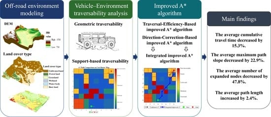
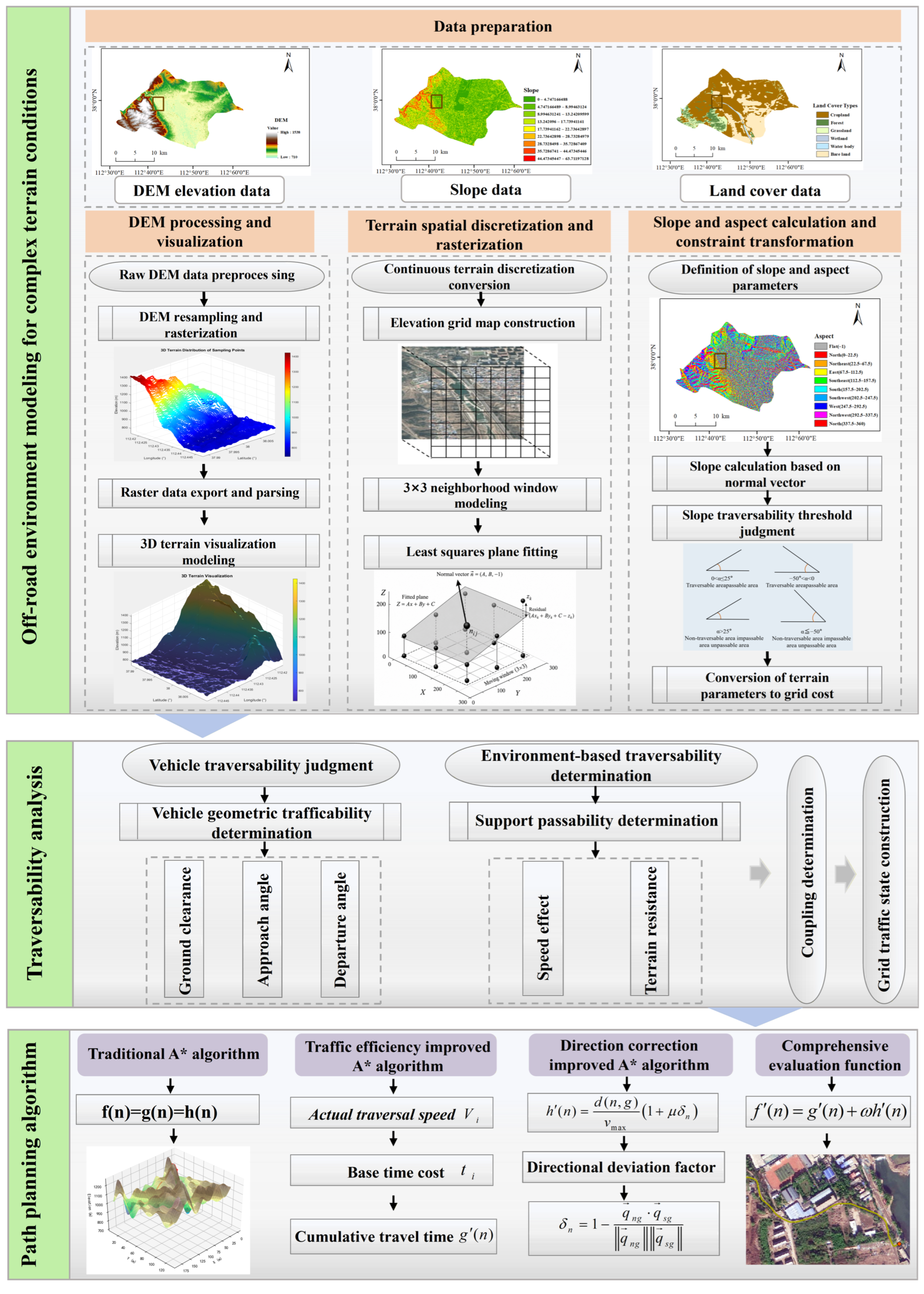
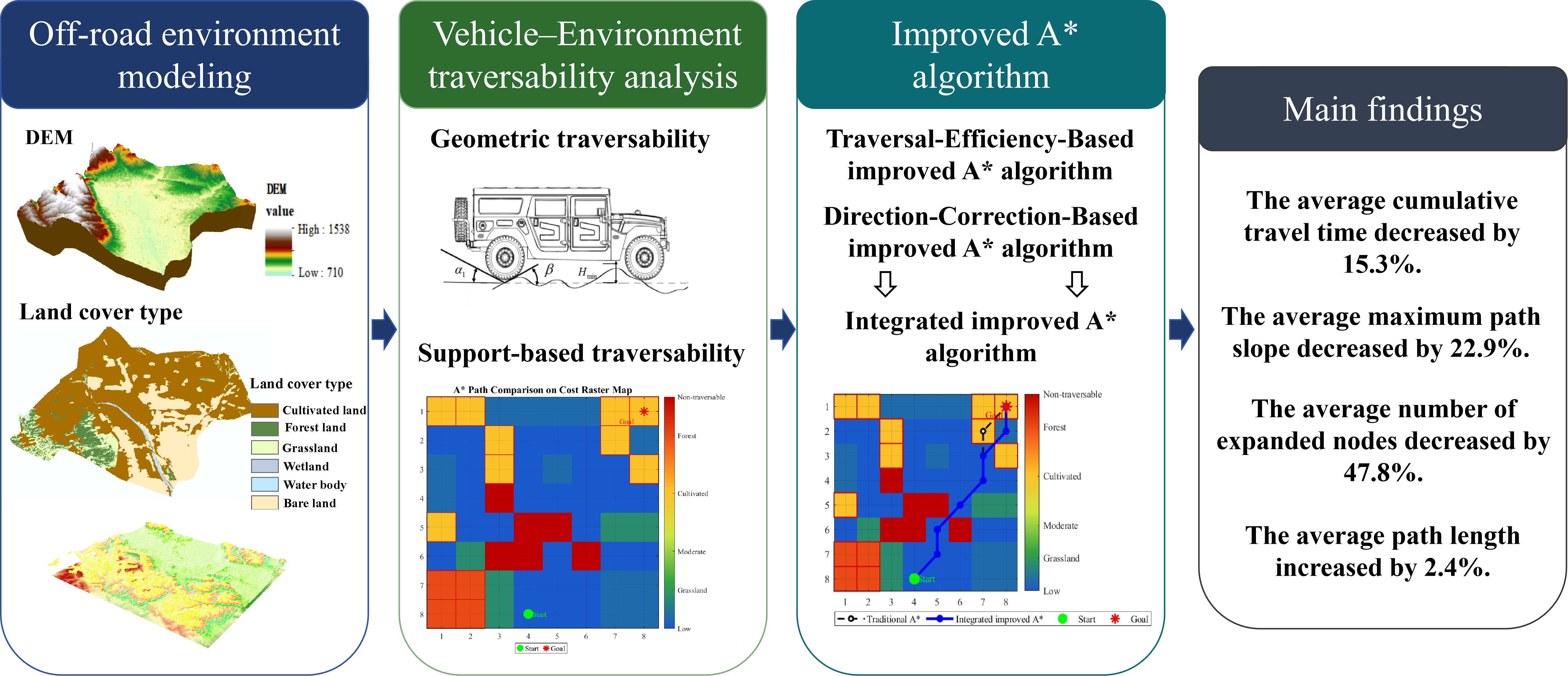
Based on the above analysis, this study aims to develop an off-road path-planning method for complex terrain surfaces by integrating real terrain environmental data with environment–vehicle traversability analysis. First, an off-road environment model is constructed using DEM and land cover data from a study area in Jiancaoping District, Taiyuan, and the least-squares plane fitting method is adopted to improve the calculation accuracy of slope and aspect. Second, environment–vehicle traversability analysis is performed from the perspectives of geometric traversability and support-based traversability. The minimum ground clearance, approach angle, and departure angle are used to characterize the geometric traversability of the vehicle, while surface bearing conditions, surface resistance, and the maximum driving speed under different surface conditions are used to represent the support-based traversability of the vehicle. These factors are then uniformly mapped into risk constraints and environmental costs. Finally, the traditional A* algorithm is improved in two aspects. First, an A*-based actual cost function considering traversal efficiency is designed, in which slope correction and surface resistance factors are incorporated into the accumulated path-cost calculation to improve actual traversal efficiency. Second, a direction-corrected heuristic function is proposed to enhance the goal-directedness of path search under complex terrain conditions and reduce ineffective node expansion, thereby forming an integrated improved A* algorithm. The overall technical route of this study is shown in Figure 1.

2. Materials and Methods

2.1. Study Area and Data Sources

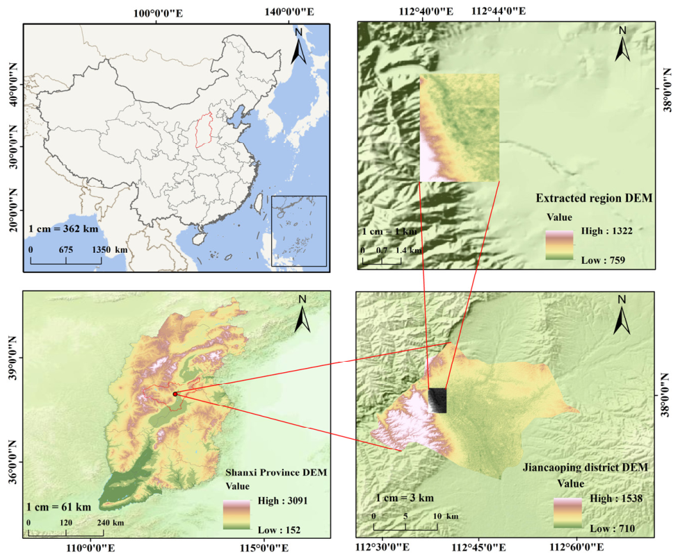
To enable path planning in complex off-road environments, the terrain information of the study area must first be modeled. The experimental region is selected as the mountainous area southwest of North University of China in Jiancaoping District, Taiyuan, Shanxi Province, China, with spatial boundaries defined by the coordinates (112.378° E, 38.008° N) to (112.453° E, 37.954° N), as illustrated in Figure 2. The terrain of this area exhibits significant undulations and diverse surface cover types, providing a representative natural environment that reflects the challenges encountered by unmanned ground vehicles (UGVs) during off-road traversal.

Three types of data and two software tools are employed in this study: satellite remote sensing data (Landsat), digital elevation model (DEM) data, and land cover data, as well as ArcGIS and MATLAB. A detailed summary is provided in

Table 1. Environmental data information.

Data Type	Source	Year	Spatial Resolution
DEM Data	Geospatial Data Cloud (https://www.gscloud.cn/)	2020	30 M
Landsat Data	Geospatial Data Cloud (https://www.gscloud.cn/)	2020	30 M
Land Cover Data	Tianditu (https://www.tianditu.gov.cn/)	2020	30 M
Data Processing Software	ArcGIS 10.8	-	-
Algorithm Implementation Software	MATLAB R2024b	-	-

.

The preprocessing procedures included projection transformation, study-area clipping, raster alignment, and resampling to a unified raster grid, thereby ensuring spatial consistency between the DEM and land cover datasets. The 2020 land cover data were used to identify surface categories, generate the traversability mask, assign surface velocity influence coefficients, and construct the environmental cost matrix. The DEM data were used to represent regional-scale terrain relief for slope and aspect extraction.

2.2. DEM Data Processing and Terrain Visualization Modeling

To construct an off-road environment model suitable for unmanned ground vehicle path planning, the digital elevation model (DEM) of the study area was used as the fundamental data source. DEM data can effectively represent the surface elevation variations of the study area and provide an essential basis for subsequent environment modeling and path planning analysis. However, raw DEM data are typically stored in a geographic coordinate system, and their data organization is not fully consistent with the regular computational space required for path planning. If such data are directly used for subsequent modeling, errors in distance calculation and inconsistencies in local analysis scales may be introduced. Therefore, before path planning is performed, standardized preprocessing of the raw DEM data is required to ensure the accuracy of the environment modeling results and the consistency of subsequent algorithm implementation.

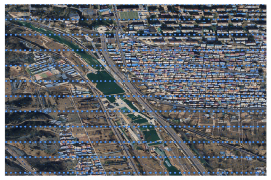
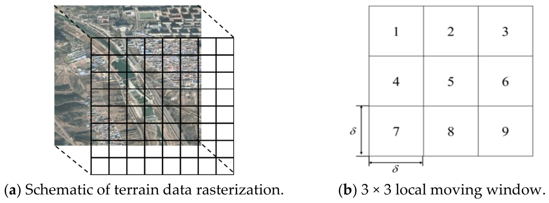
Specifically, projection transformation was first performed on the raw DEM data, through which the data were unified into a planar coordinate system suitable for metric distance calculation and spatial analysis. The DEM was then clipped according to the boundary of the study area, and irrelevant regions were removed to reduce the computational burden caused by redundant data. On this basis, the DEM data were resampled to ensure that each raster cell corresponded to a unique spatial location and elevation value, thereby forming a discretized environmental matrix that could be directly used for subsequent terrain analysis, as shown in Figure 3.

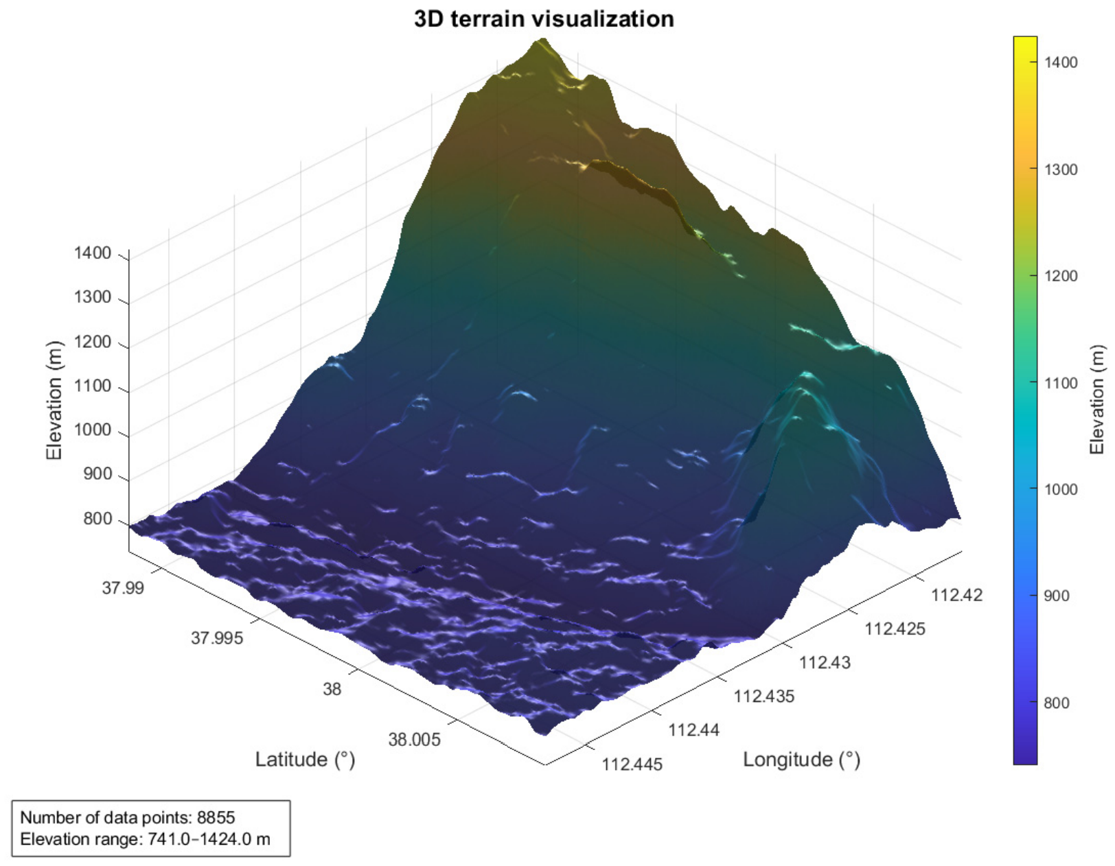
After DEM preprocessing and raster construction were completed, the reconstructed elevation data and longitude–latitude data were further imported into MATLAB through Excel files for parsing, and a three-dimensional terrain visualization of the study area was generated, as shown in Figure 4. The 3D terrain map provides an intuitive representation of the spatial distribution of steep slopes, gentle slopes, and relatively flat areas within the experimental region, thereby facilitating an overall understanding of the terrain undulation characteristics of the study area. The 3D terrain visualization was mainly used to verify the rationality of the DEM preprocessing results and to provide a reference for subsequent terrain spatial discretization, slope and aspect calculation, and environmental constraint extraction.

In summary, the DEM data were transformed from raw elevation information into a standardized raster terrain model, through which a unified representation of the terrain information in the study area was achieved. This transformation provides a reliable data basis for subsequent terrain parameter extraction, environment–vehicle traversability analysis, and path-planning cost modeling.

2.3. Terrain Spatial Discretization and Raster Representation

The terrain surface in off-road environments can be regarded as a continuous three-dimensional Euclidean space, whereas algorithms such as A* essentially rely on discrete state spaces for search and cost calculation. Therefore, these algorithms cannot be directly applied to continuous terrain surfaces. The continuous terrain environment needs to be transformed into a structured discrete representation. Based on the previously acquired and preprocessed DEM data, an elevation raster map was adopted as the fundamental modeling form for the off-road environment. By overlaying a regular grid on the surface of the study area, the continuous terrain was divided into grid cells with uniform size, and each grid cell was assigned a unique elevation attribute, as shown in Figure 5.

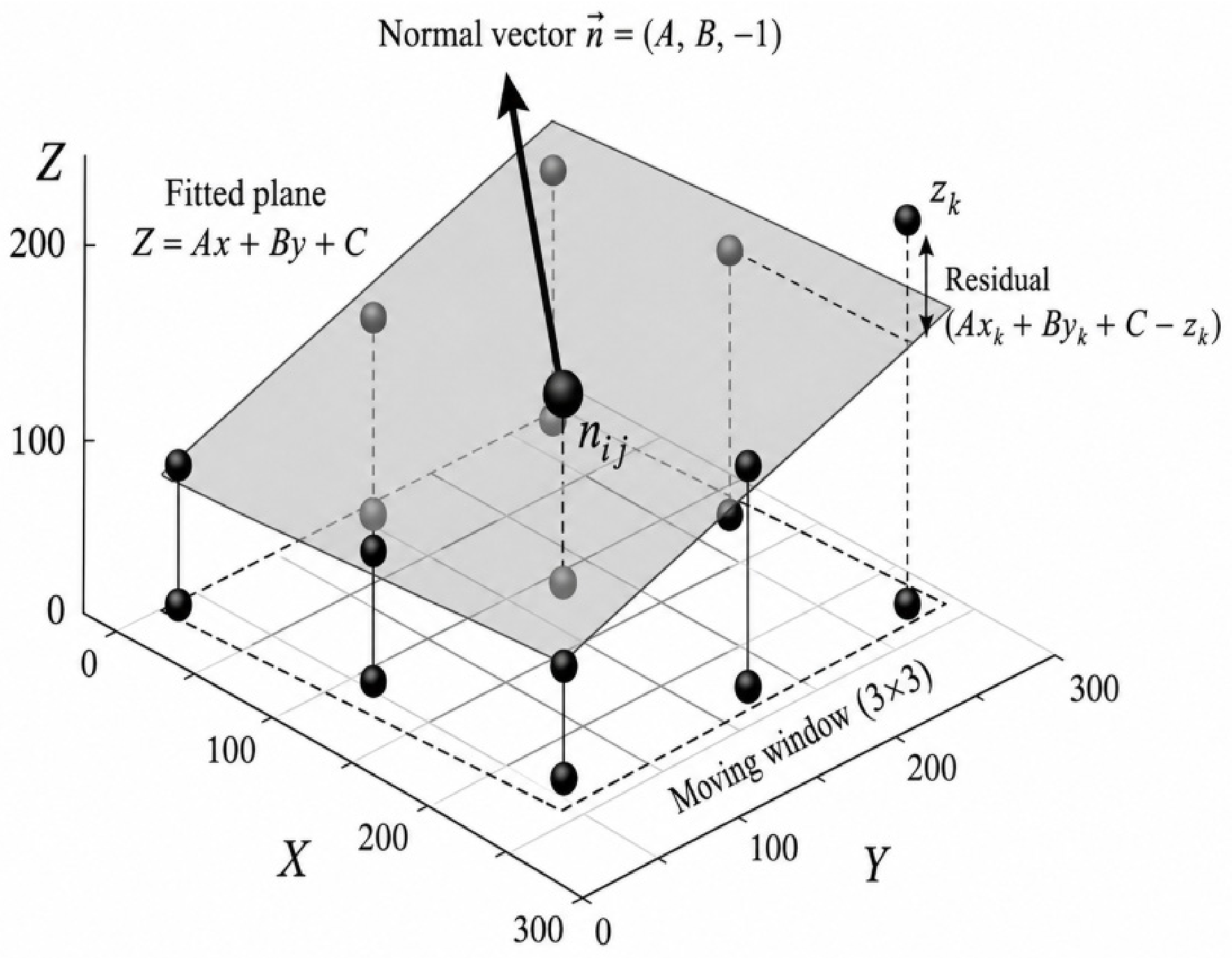
Slope and aspect are key parameters for characterizing terrain relief and slope orientation, and they directly affect the driving safety, stability, and traversal efficiency of off-road vehicles. Considering that DEM data may contain noise introduced during acquisition, interpolation, and rasterization, the direct use of the finite difference method for gradient calculation may lead to large fluctuations in local results. To improve the smoothness and robustness of terrain parameter extraction, a least-squares plane fitting method was introduced within a 3 × 3 neighborhood to model the local terrain surface. It is assumed that the terrain within the window can be approximately represented by a plane, which is expressed as follows:

$$Z=Ax+By+C$$

(1)

where $(x,y)$ denote the local planar coordinates, $Z$ denotes the fitted elevation value, and $A$, $B$, and $C$ are the plane parameters to be estimated. Specifically, $A$ and $B$ represent the first-order partial derivatives, namely the gradients, of the fitted plane in the x- and y-directions, respectively, while $C$ is the intercept constant. To estimate the optimal parameters, an objective function $E$ was constructed as the sum of squared residuals between the observed elevations and the fitted plane elevations for all points within the window:

$$E={\displaystyle \sum _{k=1}^N{(A{x}_k+B{y}_k+C-z_k)}^2}$$

(2)

where $N$ denotes the total number of raster cells within the local window, and $N=9$ in this study. To minimize the accumulated fitting error, the partial derivatives of the objective function with respect to $A$, $B$, and $C$ were calculated and set to zero, yielding the following normal equation system:

$$\left\{\begin{array}{l}{\displaystyle \frac{\mathsf{\partial }E}{\mathsf{\partial }A}}=2{\displaystyle \sum _{k=1}^N{x}_k}(A{x}_k+B{y}_k+C-z_k)=0\hfill \\ {\displaystyle \frac{\mathsf{\partial }E}{\mathsf{\partial }B}}=2{\displaystyle \sum _{k=1}^N{y}_k}(A{x}_k+B{y}_k+C-z_k)=0\hfill \\ {\displaystyle \frac{\mathsf{\partial }E}{\mathsf{\partial }C}}=2{\displaystyle \sum _{k=1}^N(A{x}_k+B{y}_k+C-z_k)}=0\hfill \end{array}\right.$$

(3)

By solving this system, the parameters of the locally optimal fitted plane and its normal vector can be obtained for the current window. Based on the gradient information of the fitted plane, the slope and aspect corresponding to the central raster cell can be further calculated. The slope is used to describe the inclination degree of the terrain cell, whereas the aspect is used to characterize the orientation of the slope surface. Compared with the direct finite difference method, the proposed fitting-based method can effectively suppress the influence of high-frequency noise on the calculation results, thereby allowing the derived terrain parameters to better conform to actual terrain variation patterns. Figure 6 presents a schematic illustration of local terrain plane fitting based on the least-squares method.

In summary, the transformation from continuous natural terrain to a computable environmental model was achieved through raster discretization and moving-window-based local fitting, and key terrain parameters required for subsequent traversability analysis were obtained. The above modeling results provide a reliable data basis for introducing slope constraints, constructing a vehicle–environment coupled traversability evaluation model, and designing off-road path planning algorithms. It should be noted that the 3 × 3 least-squares plane fitting method is mainly used to obtain a stable raster-scale slope representation for global path planning. Although this method can suppress high-frequency noise in DEM data, it may also smooth abrupt terrain variations and underestimate small-scale hazards, such as narrow gullies, sharp ridges, and artificial steps. Therefore, the slope derived in this study should be interpreted as the dominant terrain inclination within the local raster neighborhood rather than a complete description of all micro-topographic hazards. The generated slope map is suitable for global traversability assessment, while local obstacle avoidance and real-vehicle execution still require higher-resolution terrain data or onboard perception sensors.

2.4. Calculation Methods for Slope and Aspect

After terrain raster representation and local plane fitting were completed, the slope and aspect parameters could be further extracted to characterize terrain relief. Slope reflects the inclination degree of a terrain cell and serves as an important basis for evaluating the longitudinal uphill and downhill capability of a vehicle. Aspect describes the direction of maximum elevation descent on the slope surface and can be used to analyze the rollover risk during lateral driving. Therefore, slope and aspect are regarded as key terrain constraint factors in off-road environment modeling. The terrain slope, denoted by $T_{slope}$, is defined as the angle between the normal vector $\overrightarrow{n}$ of the fitted plane and the vertical unit vector $\overrightarrow{Z}=(0,0,1)$ in the inertial coordinate system, and it physically represents the inclination intensity of the terrain cell. Based on the vector dot-product formulation, the slope can be calculated as follows:

$$T_{slope}=\arccos \left({\displaystyle \frac{|\overrightarrow{n}\cdot \overrightarrow{Z}|}{\Vert \overrightarrow{n}\Vert \cdot \Vert \overrightarrow{Z}\Vert }}\right)=\arccos \left({\displaystyle \frac{1}{\sqrt{A^2+B^2+1}}}\right)$$

(4)

The calculated $T_{slope}$ is expressed in degrees. To maintain consistency between terrain modeling and experimental evaluation, a unified conservative slope threshold was adopted in the proposed traversability model. Specifically, when the absolute terrain slope satisfies $\left|T_{slope}\right|>{\theta }_{lim}$, the corresponding grid cell is regarded as a high-risk or non-traversable cell in the improved path-planning cost map. In the experiments, ${\theta }_{lim}=25°$. Although uphill and downhill traversal capabilities may differ in real vehicle dynamics, this study focuses on global path planning based on raster terrain data. Therefore, a unified conservative threshold was used in the proposed method to avoid overestimating the traversability of steep terrain and to ensure consistency throughout the modeling and evaluation process.

Aspect $T_{aspect}$ is defined as the projection direction of the terrain surface normal vector on the horizontal plane, corresponding to the direction of the steepest decrease in gravitational potential energy. This parameter is essential for evaluating the lateral stability of the vehicle. Using the geometric relationship between the fitted-plane normal vector $\overrightarrow{n}=(A,B,-1)$ and the unit vector ${\overrightarrow{n}}_y=(0,1,0)$ along the north-oriented axis, the aspect angle can be calculated as follows:

$$T_{aspect}=\arccos \left({\displaystyle \frac{\overrightarrow{n}\times {\overrightarrow{n}}_y}{\Vert \overrightarrow{n}\Vert \cdot \Vert {\overrightarrow{n}}_y\Vert }}\right)$$

(5)

The calculated result should be normalized according to its quadrant so that the aspect angle falls within [0, 2π) or [0°, 360°), with north defined as 0° and clockwise rotation taken as positive. By incorporating slope and aspect information, the algorithm can accurately identify whether the vehicle is in a longitudinal climbing/descending state or a hazardous lateral-slope state, thereby ensuring the physical safety of path planning.

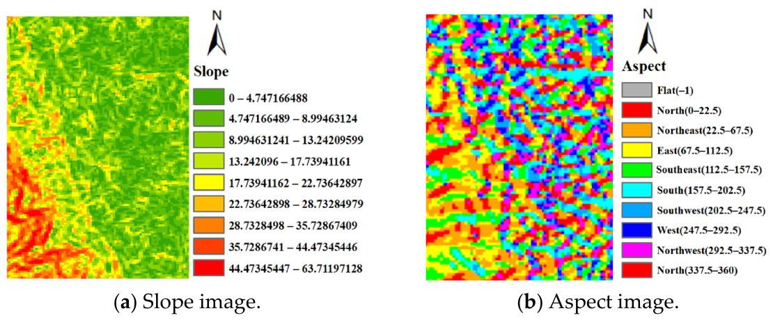
As shown in Figure 7, the study area exhibits pronounced terrain undulations, and the slope distribution shows strong spatial heterogeneity. Flat and gentle-slope areas are mainly concentrated along roads and in some farmland regions, where the slope is relatively small and favorable traversability conditions are provided. In contrast, ridges and adjacent areas exhibit larger slopes, some of which exceed the safe traversability threshold of the vehicle and therefore can be regarded as hard-constraint obstacles in path planning. The aspect results indicate that slope orientations in the study area vary considerably, suggesting that vehicles may frequently encounter lateral slope disturbances from different directions during driving. Therefore, in the subsequent traversability analysis, slope was used as the primary constraint indicator, while aspect information was incorporated to assist in evaluating vehicle attitude stability. In this way, terrain geometric features were further transformed into raster cost information readable by the path-planning algorithm.

2.5. Environment–Vehicle Coupled Traversability Analysis

In complex off-road environments, path planning is not merely a geometric obstacle-avoidance problem; rather, it is a comprehensive decision-making problem jointly determined by terrain relief, surface attributes, and the vehicle’s traversability capability. Therefore, before path planning is performed, environmental information and vehicle constraints need to be uniformly mapped into the raster space, and an environment–vehicle coupled traversability evaluation model should be established to provide a basis for subsequent cost modeling and path search.

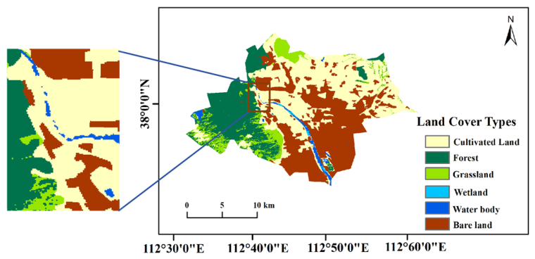
Based on the previously constructed DEM raster environment and the extracted slope and aspect information, land cover types were further introduced as surface-attribute constraints. Through interpretation of the remote sensing images of the study area, the experimental region was classified into typical land cover types, including bare land, cultivated land, grassland, forest, wetland, and water bodies, whose spatial distribution is shown in Figure 8. Different land cover types exhibit substantial differences in bearing capacity, adhesion conditions, and surface resistance, and therefore can effectively characterize the spatial heterogeneity of surface conditions in off-road environments.

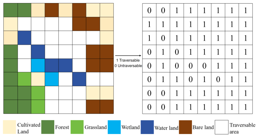
To facilitate direct use by the path-planning algorithm, the land cover data were rasterized, and each grid cell was assigned a corresponding surface-category label. Subsequently, traversability identification was performed for each surface type by incorporating vehicle traversability constraints, and a binary traversability result was generated, as shown in Figure 9. Specifically, areas that can stably support vehicle passage were retained as traversable grid cells, whereas water bodies, wetlands, and other regions that do not satisfy the traversability requirements were classified as non-traversable areas.

2.5.1. Geometric Traversability Analysis

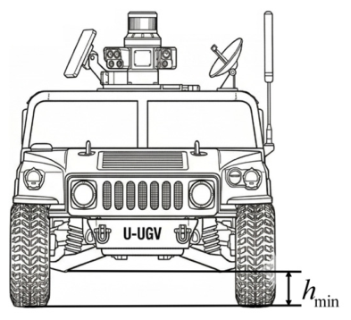
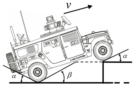
Regarding vehicle constraints, because this study aims to construct a computable environmental model for path planning rather than a highly complex vehicle dynamics simulation system, the minimum ground clearance, approach angle, and departure angle were selected as the core constraint parameters to directly characterize the geometric traversability of the vehicle, as illustrated in Figure 10 and Figure 11.

Specifically, the minimum ground clearance $h_{\min }$ is used to describe the minimum safe distance between the lowest point of the vehicle chassis and the ground. The approach angle $\alpha$ characterizes the geometric traversability of the vehicle front when entering a slope or obstacle, whereas the departure angle $\beta$ reflects the geometric traversability of the vehicle rear when leaving a slope or obstacle. If the ground clearance of the lowest point of the front overhang is denoted by $h_f$, and the horizontal distance from the front-wheel contact point to the lowest point of the vehicle front is denoted by $l_f$, while the ground clearance of the lowest point of the rear overhang is denoted by $h_r$, and the horizontal distance from the rear-wheel contact point to the lowest point of the vehicle rear is denoted by $l_r$, the approach and departure angles can be respectively expressed as follows:

$$\alpha =\arctan \left({\displaystyle \frac{h_f}{l_f}}\right)$$

(6)

$$\beta =\arctan \left({\displaystyle \frac{h_r}{l_r}}\right)$$

(7)

The above parameters can be determined from the vehicle structural dimensions or the technical manual of the prototype vehicle. Furthermore, by combining the local slope information obtained from the plane-fitting method described above, the elevation difference between two adjacent grid cells is denoted as $\mathrm{\Delta }{z}_{ij}$ and their horizontal distance is denoted as $d_{ij}$. The local slope angle can then be expressed as follows:

$${\theta }_{ij}=\arctan \left({\displaystyle \frac{\left|\mathrm{\Delta }{z}_{ij}\right|}{d_{ij}}}\right)$$

(8)

By incorporating the slope and elevation variation information obtained from the $3\times 3$ neighborhood-based plane fitting, geometric traversability evaluation was performed for each grid cell. If the local slope or obstacle characteristics of a grid cell exceed the geometric traversability limits of the vehicle, the grid cell is regarded as a geometrically non-traversable region and is excluded as a hard constraint during path planning.

2.5.2. Support-Based Traversability Analysis

In addition to geometric traversability, support-based traversability is also a critical factor affecting the mobility of off-road vehicles. Support-based traversability mainly reflects whether sufficient ground support and tire–surface adhesion can be obtained under different surface-medium conditions, and it is closely associated with bearing capacity, surface roughness, and vegetation coverage. To quantify the influence of surface conditions on vehicle mobility, a speed influence coefficient $\eta (x)$ was introduced, with its value constrained within $0\le \eta (x)\le 1$. A larger $\eta (x)$ indicates lower surface resistance and higher traversal efficiency, whereas a smaller $\eta (x)$ implies greater driving resistance on the corresponding surface type. For vegetation-covered areas, a piecewise function was adopted to describe the speed influence coefficient under different vegetation densities:

$$\eta (x)=\left\{\begin{array}{l}1.0,\hspace{1em}\mathrm{grass} \mathrm{or} \mathrm{crops} (\mathrm{low} \mathrm{resistance})\hfill \\ 0.7,\hspace{1em}\mathrm{shrubs} (\mathrm{medium} \mathrm{resistance})\hfill \\ 0.5,\hspace{1em}\mathrm{sparse} \mathrm{trees} (\mathrm{high} \mathrm{resistance}, \mathrm{spacing} \ge 6 \mathrm{m})\hfill \\ 0.1,\hspace{1em}\mathrm{dense} \mathrm{trees} (\mathrm{extremely} \mathrm{high} \mathrm{resistance}, 4 \mathrm{m}\le \mathrm{spacing}<6 \mathrm{m})\hfill \\ 0,\hspace{1em} \mathrm{spacing} \le 4 \mathrm{m} \left(\mathrm{impassable}\right)\hfill \end{array}\right.$$

(9)

Because water bodies and wetlands have extremely low bearing capacity, sufficient ground support can hardly be obtained by vehicles, making them highly susceptible to sinking or skidding. Therefore, these areas were directly classified as non-traversable regions, and $\eta (x)=0$ was assigned. Based on the above rules, a mapping relationship between land cover types and speed influence coefficients was established, as shown in

Table 2. Mapping relationship between land cover types and velocity influence coefficients.

Land Use Type	Surface Attribute	Velocity Influence Coefficient	Map Color
Bare land	Road/Hard surface	1.0	Brown
Cultivated land	Unvegetated soil	0.8	Orange
Grassland	Grassland	0.5	Light green
Forest	Forest	0.1	Green
Wetland	Marsh	0	Blue
Water body	River	0	Dark blue

. It should be noted that the speed influence coefficient is not a fixed physical constant for a given surface type, but rather a relative traversal-efficiency parameter designed for path-planning cost modeling. The traversability cost of off-road robots can generally be estimated based on surface categories, experimental data, or robot motion data [26].

To achieve a unified representation of environmental information and vehicle constraints, land cover types and vehicle traversability parameters were mapped onto a regular raster space, and a raster state matrix was constructed as follows:

$$S(x,y)=[\eta (x,y),G(x,y)]$$

(10)

In this equation, $\eta (x,y)$ denotes the surface support-based traversability, whereas $G(x,y)$ represents the vehicle geometric traversability evaluation result.

First, a binary traversability mask matrix was introduced to perform hard-constraint screening of the study area:

$$M(x,y)=\left\{\begin{array}{l}1, \eta (x,y)>0 and G(x,y)=1\hfill \\ 0, otherwise\hfill \end{array}\right.$$

(11)

This step ensures that the path-planning algorithm does not search in regions that are geometrically inaccessible or insufficiently supported by the ground, and the corresponding result is shown on the right side of Figure 9. Within the traversable regions satisfying $M(x,y)=1$, vehicle traversal efficiency still varies significantly under different surface conditions. Therefore, a physical resistance cost was introduced to quantify traversal difficulty, which is defined as the relative time cost required for the vehicle to travel a unit distance:

$$C_{env}(x,y)={\displaystyle \frac{1}{\eta (x,y)}}$$

(12)

Specifically, bare land corresponds to $C_{env}=1$ and is used as the reference traversable environment; grassland corresponds to $C_{env}=2$, indicating that its traversal time cost is approximately twice that of hard-surface roads; and forest areas are treated as high-cost soft obstacles in path planning because of their extremely large resistance. Finally, the physical attribute vector of each grid node can be expressed as follows:

$$P(x,y)=[M(x,y),C_{env}(x,y)]$$

(13)

Through the above environment–vehicle coupled traversability modeling process, a unified mapping among land-cover semantic information, vehicle geometric constraints, and path-planning cost representation was achieved. Under the premise that vehicle passage safety is ensured, the proposed method can preferentially guide the path-planning algorithm to avoid water bodies, wetlands, and high-risk regions, while selecting surface types with higher traversal efficiency. Consequently, a reliable environmental constraint basis is provided for subsequent optimal path search.

2.6. Principle of the Traditional A* Algorithm

The A* algorithm is a classical heuristic graph-search algorithm and has been widely used in global path planning for unmanned ground vehicles because of its heuristic guidance and optimality guarantee. Its core evaluation function is defined as follows:

$$f(n)=g(n)+h(n)$$

(14)

In this equation, $g(n)$ denotes the actual cost from the start node to the current node, $h(n)$ represents the heuristic estimated cost from the current node to the target node, and $f(n)$ denotes the overall evaluation function.

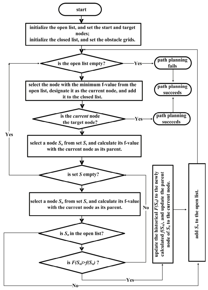
The search process is completed by maintaining an Open list and a Closed list. The Open list is used to store nodes to be expanded, whereas the Closed list is used to record visited nodes and non-traversable nodes. During the search process, the node with the minimum $f(n)$ value is repeatedly selected from the Open list for neighborhood expansion until the target node is reached or the Open list becomes empty. The basic workflow of the traditional A* algorithm is shown in Figure 12.

Under the eight-neighborhood search mode, the node cost recurrence relation of the traditional A* algorithm can be expressed as follows:

$$g(n)=g(p)+c(n,p)$$

(15)

Here, $c(n,p)$ denotes the grid movement cost between the current node and its parent node. When movement occurs in the horizontal or vertical direction, the movement distance $d(n,p)$ is equal to the grid side length $S$. When diagonal movement occurs, $d(n,p)$ is equal to $\sqrt{2}S$. The heuristic function is generally formulated using the Euclidean distance to ensure search-direction consistency and optimality.

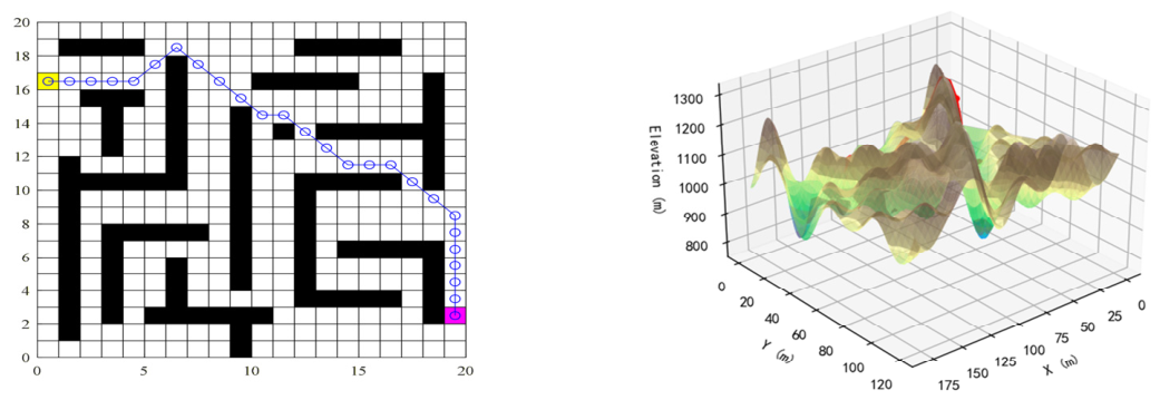
The grid map generated by the traditional A* algorithm based on the raster method and the corresponding three-dimensional terrain path-planning result are shown in Figure 13. The grid states can be simplified into two categories: obstacle cells and free cells. Obstacle cells are assigned a value of 1, represented in black, and recorded in the Closed list, whereas free cells are assigned a value of 0 and represented in white. The blue line with circular markers represents the path planned by the traditional A algorithm, while the yellow and magenta markers indicate the start and target points, respectively.

The traditional A* algorithm is well suited to structured road environments; however, in complex off-road environments, geometric distance alone is used as the search criterion, making it difficult to reflect the effects of terrain slope variation, land-cover heterogeneity, and vehicle traversability constraints on path quality. As a result, paths may be generated that are relatively short in distance but inefficient or even unsafe for vehicle traversal. Therefore, the environment–vehicle coupled traversability results constructed above need to be further incorporated into the path-search process, so that the traditional A* algorithm can be improved.

2.7. Design of the Improved A* Algorithm

2.7.1. Constraint Information Representation for Off-Road Environments

To enable the slope, surface type, and traversability results obtained above to be directly incorporated into the A* search process, a risk-factor matrix and an environmental-factor matrix were constructed in the grid space, through which environmental information was mapped into path-planning constraints.

Specifically, the risk-constraint matrix was used to represent strictly non-traversable regions. Let $M_i$ denote the binary traversability mask obtained above. The risk-constraint matrix was defined as follows:

$$R_i=1-M_i$$

(16)

When $R_i=1$, the corresponding grid cell is identified as a risky or non-traversable cell and should be directly excluded as an obstacle during path search. When $R_i=0$, the grid cell is considered to satisfy the basic traversability condition. Meanwhile, to describe the traversal difficulty under different surface conditions within traversable regions, an environmental cost matrix was introduced as follows:

$$E_i=\left\{\begin{array}{ll}{\displaystyle \frac{1}{{\eta }_i}},\hfill & M_i=1\hfill \\ +\infty ,\hfill & M_i=0\hfill \end{array}\right.$$

(17)

In this equation, ${\eta }_i$ denotes the surface speed influence coefficient of grid cell $i$. Accordingly, the risk-constraint matrix is used to eliminate non-traversable regions, whereas the environmental cost matrix is used to characterize local resistance variations within traversable regions. Together, these two matrices constitute the environmental constraint basis for the improved A* algorithm.

2.7.2. Improved A* Cost Function Based on Traversal Efficiency

In the traditional A* algorithm, the actual cost is constructed by accumulating geometric distances, and its optimization objective is essentially to minimize the path length. However, in complex off-road environments, path quality is determined not only by path length but also by the actual traversal efficiency of the vehicle under different surface types and slope conditions. Therefore, the path-planning objective was reformulated from shortest-distance minimization to shortest-travel-time minimization.

By incorporating the surface speed influence coefficient and slope information described above, the actual maximum traversable speed of grid cell $i$ was defined as follows:

$$v_i=v_0{\eta }_i\varphi ({\theta }_i)$$

(18)

In this equation, $v_0$ denotes the reference speed used for traversal-time cost calculation on an ideal hard surface, ${\eta }_i$ represents the surface speed influence coefficient of grid cell $i$, ${\theta }_i$ denotes the local slope of the grid cell, and $\varphi ({\theta }_i)$ is the slope correction function, which is expressed as follows:

$$\varphi ({\theta }_i)=\left\{\begin{array}{ll}1-{\displaystyle \frac{{\theta }_i}{{\theta }_{lim}}},\hfill & 0\le {\theta }_i<{\theta }_{lim}\hfill \\ 0,\hfill & {\theta }_i\ge {\theta }_{lim}\hfill \end{array}\right.$$

(19)

In this equation, ${\theta }_{lim}$ denotes the allowable safe slope threshold of the vehicle. When the slope exceeds this threshold, the grid-cell speed is set to zero, and the corresponding cell is regarded as a non-traversable region. After the actual traversable speed of each grid cell is obtained, the basic travel-time cost between adjacent nodes is further defined as follows:

$$t_i={\displaystyle \frac{d_i}{v_i}}$$

(20)

In this equation, $d_i$ denotes the movement distance between the current node and its parent node. In the eight-neighborhood search mode, $d_i=S$ when the node is expanded horizontally or vertically, whereas $d_i=\sqrt{2}S$ when the node is expanded diagonally, where $S$ denotes the grid side length. Therefore, the accumulated actual cost from the start node to the current node can be directly expressed as the accumulated travel time:

$$g^{\prime }(n)=g^{\prime }(p)+t_i$$

(21)

In this equation, $g^{\prime }(p)$ denotes the accumulated travel-time cost of the parent node. The effects of surface resistance and slope have been incorporated into the actual traversable speed $v_i$ through ${\eta }_i$ and $\varphi ({\theta }_i)$, thereby making the cost function more consistent with real off-road traversal conditions.

2.7.3. Design of a Direction-Corrected Heuristic Function

After the actual cost is reformulated from a distance-based cost to a time-based cost, the heuristic function should also be made consistent with this objective. In the traditional A* algorithm, the heuristic function is usually formulated only using the Euclidean distance, which may lead to ineffective node expansions that deviate from the overall target direction in complex off-road environments. Therefore, a direction-correction term was introduced into the heuristic function to enhance the goal-directedness of the search process. The direction-corrected heuristic cost was defined as follows:

$$h^{\prime }(n)={\displaystyle \frac{d(n,q)}{v_{\max }}}\left(1+\mu {\delta }_n\right)$$

(22)

In this equation, $d(n,q)$ denotes the Euclidean distance from the current node to the target node, $v_{\max }$ represents the maximum actual driving speed among traversable grid cells in the study area, $\mu$ denotes the directional-deviation penalty coefficient, and ${\delta }_n$ represents the directional-deviation factor. The expression is given as follows:

$${\delta }_n=1-{\displaystyle \frac{{\overrightarrow{q}}_{nq}\cdot {\overrightarrow{q}}_{sq}}{‖{\overrightarrow{q}}_{nq}‖‖{\overrightarrow{q}}_{sq}‖}}$$

(23)

In this equation, ${\overrightarrow{q}}_{nq}$ denotes the direction vector from the current node to the target node, whereas ${\overrightarrow{q}}_{sq}$ represents the direction vector from the start node to the target node. When the current search direction is more consistent with the overall direction from the start node to the target node, ${\delta }_n$ becomes smaller, and the heuristic cost is reduced. Conversely, the heuristic cost is increased, thereby reducing ineffective searches that deviate excessively from the overall target direction. The direction-deviation penalty is used only as a soft heuristic guidance to reduce redundant node expansion away from the overall start-to-goal direction. It does not impose a straight-line constraint, because the accumulated cost $g^{\prime }(n)$ is still determined by terrain slope, surface resistance, and traversable speed, while non-traversable cells are excluded by the risk-constraint matrix. Therefore, when steep slopes, high-resistance areas, or obstacles exist along the direct direction, the algorithm can still select a safer detour.

2.7.4. Comprehensive Evaluation Function

By integrating the accumulated travel-time cost and the direction-corrected heuristic cost described above, the comprehensive evaluation function of the improved A* algorithm is defined as follows:

$$f^{\prime }(n)=g^{\prime }(n)+\omega h^{\prime }(n)$$

(24)

In this equation, $g^{\prime }(n)$ denotes the accumulated travel-time cost from the start node to the current node, $h^{\prime }(n)$ represents the direction-corrected heuristic cost from the current node to the target node, and $\omega$ is the heuristic weighting coefficient. The proposed function follows the classical A* evaluation structure, but reformulates the accumulated cost from geometric distance to travel time, thereby incorporating surface resistance and slope effects into the search process. The heuristic term estimates the remaining travel time based on the Euclidean distance and the maximum traversable speed, while the direction-deviation factor improves the goal-directedness of the search. The weighting coefficient $\omega$ is used to balance path quality and search efficiency. When the surface coefficient and slope correction are both equal to 1, the direction penalty is removed, and $\omega =1$, the proposed function reduces to the conventional A* form under a time-equivalent cost representation. The pseudocode of the integrated improved A* algorithm is presented in

Table 3. Pseudocode of the comprehensive improved A* algorithm.

Pseudocode of the comprehensive improved A* algorithm

Input: Grid map, risk-constraint matrix R, surface speed influence coefficient $\eta$, slope $\theta$, start node s, target node q, parameters $v_0$, ${\theta }_{lim}$, $\mu$, and $\omega$ 1.   $Open=\left\{s\right\}$, $Closed\ne \varnothing$, $g^{\prime }(s)=0$ 2.   while $Open\ne \varnothing$ do 3.           n = argmin $x\in Open$[$g^{\prime }(x)$+$\omega$ $h^{\prime }(x)$] 4.           if n = q then 5.                 return reconstructed path 6.           end if 7.           Move n from Open to Closed 8.           for each $m\in Neighbors(n)$ do 9.                 if m$\in Closed$ or R(m) = 1 then continue 10.               $\varphi ({\theta }_m)=max(\theta ,1-\left|{\theta }_m\right|/{\theta }_{lim})$ 11.               $v(m)=v_0\cdot \eta (m)\cdot \varphi ({\theta }_m)$ 12.               if $v(m)\le 0 then continue$ 13.               $g_{new}=g^{\prime }(n)+d(n,m)/v(m)$ 14.               ${\delta }_m=1-cos(q_{mg},q_{sg})$ 15.               $h^{\prime }(m)=d(m,q)/v_{\max }\cdot (1+\mu {\delta }_m)$ 16.               if $m\notin Open or{ \mathrm{g}}_{new}<g^{\prime }(m) then$ 17.                     $g^{\prime }(m)=g_{new}$ 18.                     $parent(m)=n$ 19.                     Add m to Open 20.               end if 21.         end for 22. end while Output: planned path or failure

.

2.8. Experimental Setup and Evaluation Metrics

To verify the effectiveness of the proposed improved A* algorithm in complex off-road environments, path-planning results under identical start–target conditions were selected for comparative analysis. The comparison methods were designed as controlled baselines and ablation variants to evaluate the contribution of traversal-efficiency modeling and direction-corrected heuristic search, rather than as an exhaustive benchmark of all state-of-the-art path-planning algorithms. In the traditional A* algorithm, the geometric distance between grid cells is used as the primary cost, and the Euclidean distance is adopted as the heuristic function; thus, the search objective is mainly represented as the shortest path in a geometric sense. In contrast, the proposed improved A* algorithm incorporates the risk-constraint matrix and environmental cost matrix into the search framework based on the previously established environment–vehicle coupled traversability analysis. Furthermore, a comprehensive evaluation function is constructed by combining a travel-time cost function with a direction-corrected heuristic function, thereby transforming path search from shortest-distance optimization into traversal-efficiency optimization under safety constraints. To improve the reproducibility of the experiments, the key vehicle and algorithm parameters used in this study are summarized in

Table 4. Vehicle and algorithm parameters used in the experiments.

Parameter	Symbol	Value	Unit	Basis/Description
Minimum ground clearance	$h_{min}$	0.13	m	Reference UGV specification
Approach angle	$\alpha$	28.5	°	Calculated from simplified vehicle geometry
Departure angle	$\beta$	28.5	°	Calculated from simplified vehicle geometry
Nominal climbing capability	-	30	°	Reference UGV specification
Safe slope threshold	${\theta }_{lim}$	25	°	Conservative threshold with safety margin
Reference speed for cost calculation	$v_0$	10	m/s	Set for traversal-time cost calculation
Grid resolution	$S$	30	m	Consistent with DEM and land-cover data
Directional penalty coefficient	$\mu$	0.80	-	Direction-corrected heuristic parameter
Heuristic weighting coefficient	$\omega$	1.00	-	Comprehensive evaluation function parameter

. The geometric parameters were determined with reference to a Husky-type research UGV platform, while $v_0$, $\mu$, and $\omega$ were used as algorithmic parameters for traversal-cost modeling and heuristic search. The reference speed $v_0$ represents the speed baseline used in the cost function rather than the physical maximum speed of a specific commercial vehicle.

In the experiments, the reference speed used for traversal-time cost calculation was set to 10 m/s, and the actual traversable speed of each grid cell was jointly determined by the surface velocity influence coefficient and the slope correction function. To ensure traversal safety under complex surface conditions, the safe slope threshold was set to 25°. The same threshold was used in both the geometric traversability model and the experimental evaluation to ensure consistency of slope constraints. This value was selected as a conservative safety threshold because the maximum climbing capability of typical research-oriented off-road UGV platforms is generally around 30°. For example, the publicly available specifications of the Clearpath Husky A300/A200 report a maximum climbing slope of 30°. Therefore, the platform limit was not directly adopted; instead, an approximately 5° safety margin was reserved, and 25° was used as the traversable safety threshold in global path planning [27]. The directional penalty coefficient in the direction-corrected heuristic function was set to 0.80 to suppress ineffective expansions that deviate from the overall target direction, and the heuristic weight in the comprehensive evaluation function was set to 1.00 to balance search efficiency and path optimality [28]. The resulting accumulated travel time reflects not only differences in path length but also the comprehensive influence of complex off-road environments on vehicle traversal efficiency.

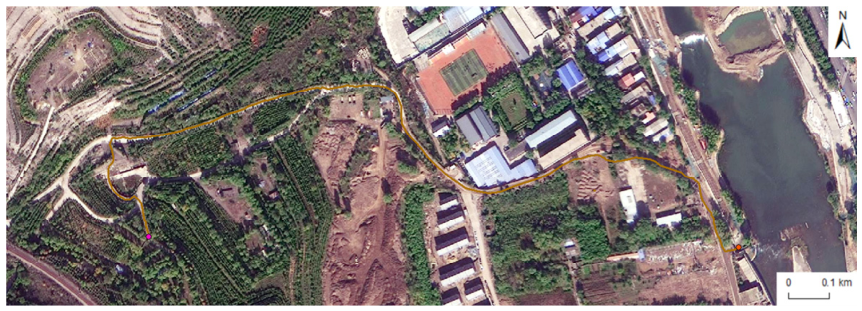
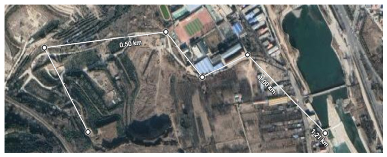
To evaluate the reliability, applicability, and execution efficiency of the proposed algorithm, five different start–target configurations were established under the same experimental scenario. The details of the selected start and target points are listed in

Table 5. Start and target configurations for the five experiments.

Experiment No	Start Point Coordinates	Target Point Coordinates	Straight-Line Distance (m)	Terrain Characteristics
1	(112.428° E, 38.003° N)	(112.427° E, 38.004° N)	196.3	Steep mountainous slope
2	(112.427° E, 38.004° N)	(112.431° E, 38.005° N)	385.7	Mixed mountainous and flat terrain
3	(112.431° E, 38.005° N)	(112.433° E, 38.003° N)	239.8	Mixed mountainous and flat terrain
4	(112.433° E, 38.003° N)	(112.435° E, 38.003° N)	204.7	Flat terrain
5	(112.435° E, 38.004° N)	(112.437° E, 38.003° N)	249.8	Gentle mountainous slope

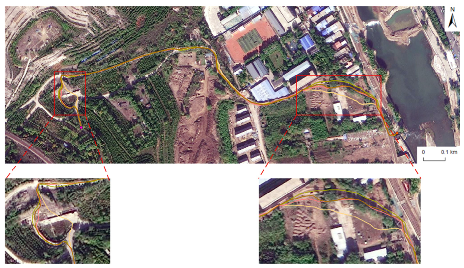
, and their spatial locations are shown in Figure 14. The path-planning results obtained by different algorithms are summarized in

Table 6. Experimental results of algorithm planning.

Algorithm	Path-Planning Result	Result Description
Traditional A* algorithm		The path is relatively short, but it locally passes through high-resistance terrain areas.
Improved A* algorithm based on traversal efficiency		The planned path better conforms to the distribution of low-resistance areas.
Improved A* algorithm based on direction correction		The overall path direction is closer to the target direction.
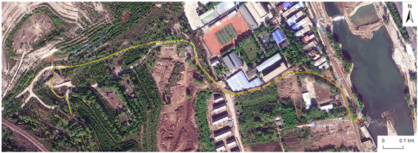
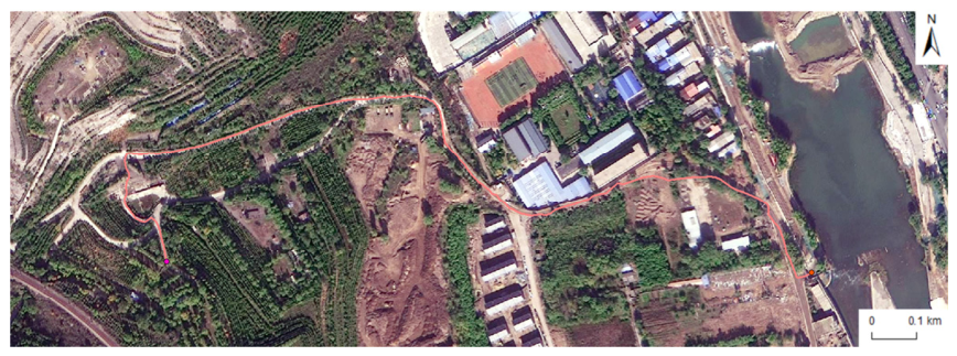
Integrated improved A* algorithm		The planned path achieves a balance between traversal efficiency and search-direction consistency.

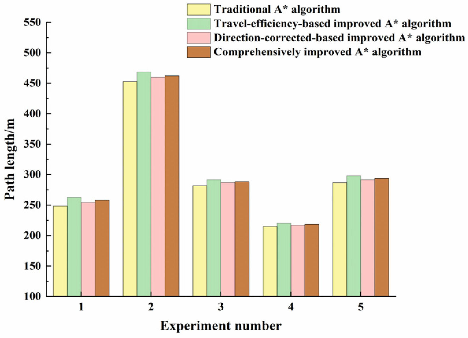
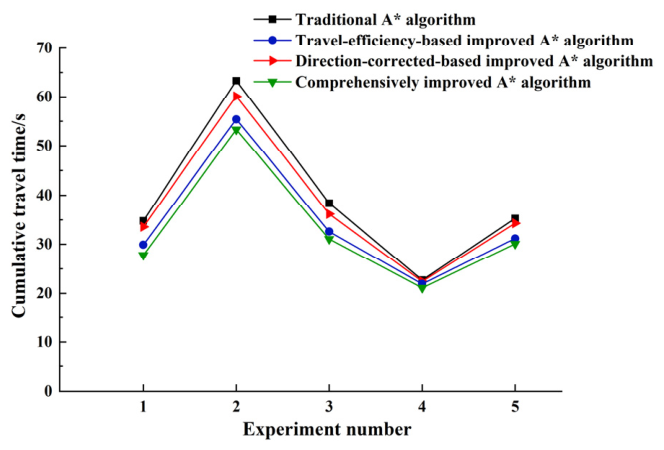
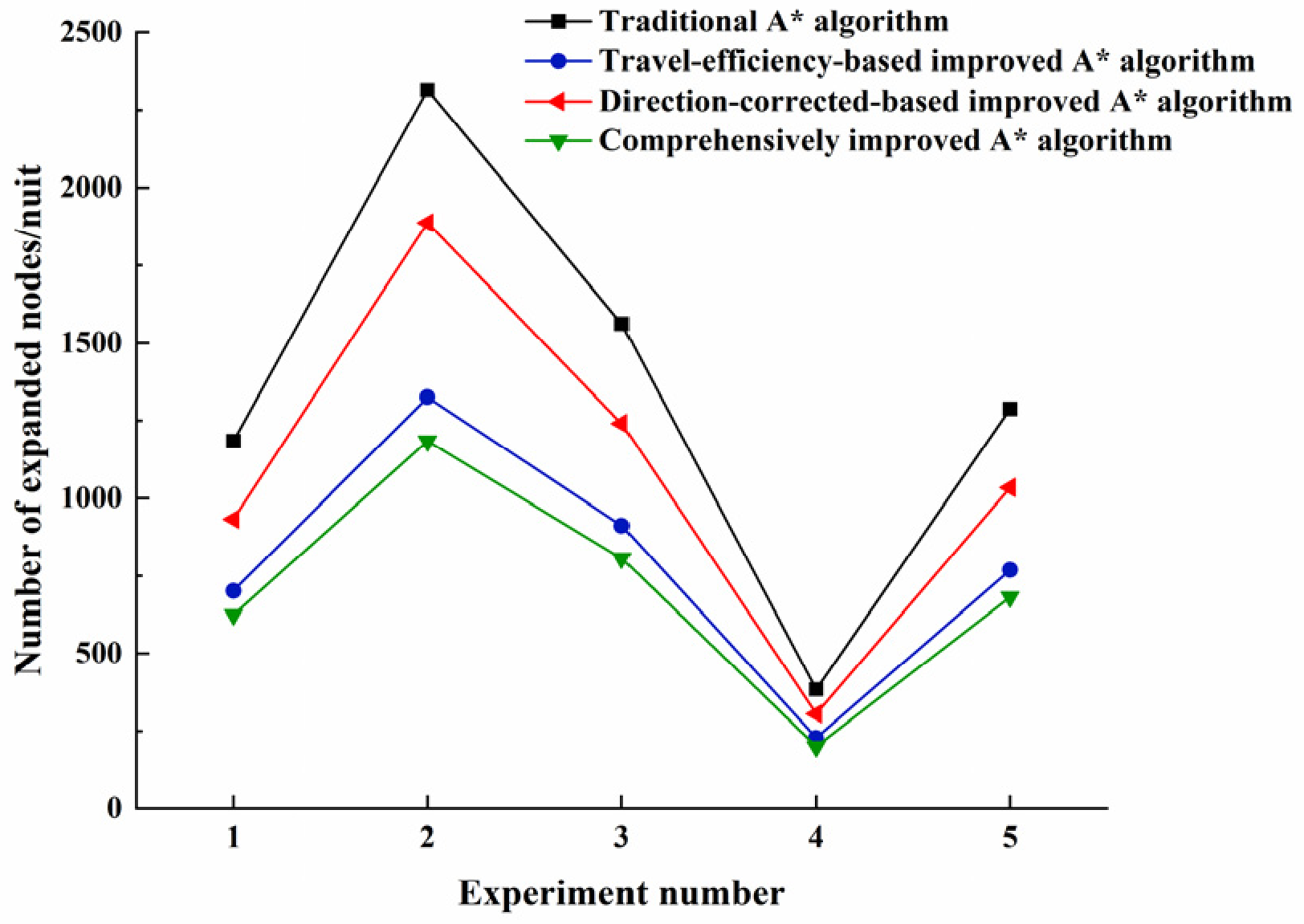
, the local enlarged path view is presented in Figure 15, and the quantitative planning results under different scenarios are provided in

Table 7. Planning scheme data of various algorithms in different scenarios.

Experiment No	Metric	Traditional A* Algorithm	Improved A* Algorithm Based on Traversal Efficiency	Improved A* Algorithm Based on Direction Correction	Integrated Improved A* Algorithm
1	Path length (m)	246.9	262.8	253.9	258.8
	Accumulated travel time (s)	34.8	29.9	33.6	27.8
	Maximum path slope (°)	27.9	22.1	24.7	21.0
	Number of expanded nodes	1179	943	694	632
2	Path length (m)	454.9	464.2	457.9	462.2
	Accumulated travel time (s)	63.3	55.4	60.1	53.3
	Maximum path slope (°)	24.9	20.8	23.2	19.6
	Number of expanded nodes	2324	1894	1332	1192
3	Path length (m)	284.4	291.2	286.8	288.1
	Accumulated travel time (s)	38.4	32.6	36.2	31.1
	Maximum path slope (°)	23.9	19.6	22.0	18.3
	Number of expanded nodes	1549	1237	934	799
4	Path length (m)	214.9	220.3	216.8	218.4
	Accumulated travel time (s)	22.7	21.9	22.4	21.1
	Maximum path slope (°)	11.5	9.4	10.6	8.8
	Number of expanded nodes	389	303	226	203
5	Path length (m)	285.9	298.3	292.1	293.8
	Accumulated travel time (s)	35.3	31.2	34.3	30.1
	Maximum path slope (°)	22.0	17.9	20.3	17.2
	Number of expanded nodes	1294	1029	772	676

.

3. Results

Experimental Results and Quantitative Comparison

Based on the terrain data, the planning results obtained in this study show good rationality in terms of path feasibility and environmental adaptability. As shown in Table 5, the improved A* algorithm based on traversal efficiency and the improved A* algorithm based on direction correction exhibit certain advantages in traversal-efficiency optimization and search guidance, respectively. In contrast, the integrated improved A* algorithm achieves the best performance in accumulated travel time and maximum path slope control while only causing a limited increase in path length, indicating that this method can more effectively meet the requirements of path planning in complex off-road environments.

To intuitively compare the planning performance of different algorithms, the results in Table 6 were analyzed from four aspects: path length, accumulated travel time, maximum path slope, and number of expanded nodes. Among these metrics, accumulated travel time is defined as the sum of the travel times between adjacent nodes along the path and is used to characterize the actual traversal efficiency in complex off-road environments.

As indicated by Table 6 and the related figures, the traditional A* algorithm produces shorter paths in most scenarios, suggesting that it has certain advantages in geometric-distance optimization. However, because surface traversal efficiency and slope constraints are not fully considered, its accumulated travel time and maximum path slope are generally higher. By contrast, the proposed improved method can more effectively avoid high-resistance and high-slope regions while maintaining overall path compactness, thereby improving the actual traversability of the planned path.

As shown in Figure 16, the four algorithms exhibit relatively small differences in path length across the five experimental scenarios. In terms of path length, the integrated improved A* algorithm increases the path length by only approximately 2.4% compared with the traditional A* algorithm, indicating that the introduction of environmental constraints does not result in significant detours.

As shown in Figure 17, the algorithms differ noticeably in accumulated travel time, with the integrated improved A* algorithm achieving the lowest values in all five scenarios. In terms of accumulated travel time, the integrated improved A* algorithm achieves an average reduction of approximately 15.3% compared with the traditional A* algorithm, indicating that a path with a shorter geometric distance does not necessarily correspond to higher off-road traversal efficiency. Instead, the time-cost function based on traversal-efficiency modeling can guide the path search more effectively.

As shown in Figure 18, the integrated improved A* algorithm consistently produces paths with lower maximum slopes than the other algorithms. In terms of maximum path slope, the integrated improved A* algorithm achieves an average reduction of approximately 22.9% compared with the traditional A* algorithm, with more pronounced advantages in steep mountainous slopes and mountain–flat terrain transition scenarios. This result indicates that the proposed method can effectively suppress the occurrence of local high-slope path segments and enhance the adaptability of the planned path to complex terrain.

As shown in Figure 19, the integrated improved A* algorithm requires fewer expanded nodes than the other algorithms in all five scenarios. In terms of the number of expanded nodes, the integrated improved A* algorithm achieves an average reduction of approximately 47.8% compared with the traditional A* algorithm, and the decrease is more evident in steep mountainous slopes and mountain–flat terrain transition scenarios. This finding suggests that the proposed method can effectively reduce redundant node expansion during path search and narrow the ineffective search range, thereby improving search efficiency in complex off-road environments.

Overall, the traditional A* algorithm places greater emphasis on geometric shortest-distance optimization, whereas the proposed integrated improved A* algorithm focuses more on comprehensive traversal performance in complex off-road environments. The results show that, with only a limited increase in path length, the accumulated travel time, maximum path slope, and number of expanded nodes are effectively controlled. Therefore, the proposed method can generate safer and more reasonable off-road paths while reducing redundant expansion during the search process, demonstrating superior overall planning performance.

4. Discussion

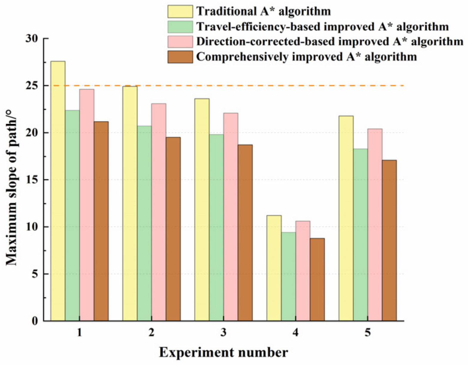
The experimental results show that, in complex off-road environments, the shortest geometric path does not necessarily provide the best traversal performance. The traditional A* algorithm mainly uses geometric distance as the search cost and therefore tends to ignore terrain slope, surface resistance, and vehicle traversability constraints. As a result, although its planned paths are relatively short, they may pass through steep or high-resistance areas, leading to longer accumulated travel time and higher maximum path slope. In contrast, the integrated improved A* algorithm proposed in this study slightly increases the path length but effectively reduces travel time, maximum slope, and the number of expanded nodes. This indicates that the proposed method achieves a better balance among path compactness, traversal efficiency, terrain safety, and search efficiency.

These results confirm that off-road path planning should be treated as a comprehensive optimization problem rather than a simple shortest-path search. In this study, geometric traversability constraints, including slope threshold, minimum ground clearance, approach angle, and departure angle, are used to exclude unsafe areas before path search. Meanwhile, the surface speed influence coefficient and slope correction function are introduced into the actual cost function, so that the influence of different land cover types and terrain slopes can be expressed as traversal-time cost. Compared with previous studies that mainly focused on DEM-based terrain representation, land-cover classification, or binary traversable/non-traversable identification, the proposed method further quantifies the traversal-efficiency differences within traversable regions. In addition, the direction-corrected heuristic function improves the goal-directedness of the search process and reduces ineffective node expansion. Therefore, the proposed algorithm transforms the planning objective from geometric shortest-distance optimization to traversal-efficiency optimization under safety constraints.

However, several limitations remain. First, although the 3 × 3 least-squares plane fitting method improves the robustness of slope estimation, it may smooth abrupt terrain changes and underestimate local hazards when the terrain variation occurs within a scale smaller than the DEM resolution. Therefore, the current terrain model is more suitable for global path planning than for direct local motion execution. Second, the spatial resolution of DEM and land cover data may affect the accuracy of terrain-cost calculation and traversability classification. Third, parameters such as the surface speed influence coefficient, safe slope threshold, and directional penalty coefficient still involve empirical assumptions and require further calibration through real-vehicle experiments. Future work will incorporate higher-resolution terrain data, LiDAR or vision-based local perception, real-vehicle tests, and real-time environmental information to improve the robustness and practical applicability of the proposed method in real off-road scenarios.

5. Conclusions

To address the insufficient consideration of terrain slope and surface traversal resistance in the traditional A* algorithm under complex off-road environments, an integrated improved A* path-planning method was proposed. In this method, an off-road environment model is constructed based on DEM and land cover data, and vehicle traversability is analyzed from the perspectives of geometric traversability and support-based traversability. The surface speed influence coefficient and slope correction term are incorporated into the actual cost function, while a direction-corrected heuristic function is combined to improve traversal efficiency and goal-directedness during path search. Experimental validation was conducted in Jiancaoping District, Taiyuan, and the following conclusions were obtained:

(1) The proposed method can comprehensively consider terrain slope, surface type, and vehicle geometric traversability constraints, thereby effectively avoiding high-slope and high-resistance regions and generating planned paths that better satisfy the practical traversal requirements of complex off-road environments.

(2) Compared with the traditional A* algorithm, the improved algorithm reduces the accumulated travel time by approximately 15.3% on average while increasing the path length by only approximately 2.4% on average, indicating that traversal efficiency can be improved while path compactness is maintained.

(3) The improved algorithm reduces the maximum path slope by approximately 22.9% on average and decreases the number of expanded nodes by approximately 47.8% on average, demonstrating that terrain safety can be enhanced, ineffective node searches can be reduced, and planning efficiency can be improved.

In summary, the proposed method achieves the coordinated optimization of path compactness, traversal efficiency, and terrain safety, demonstrating better applicability than the traditional A* algorithm in complex off-road environments. Future work will further calibrate traversal cost parameters using real-vehicle experimental data, and vehicle dynamic constraints and real-time environmental perception information will be introduced to improve the robustness and engineering applicability of the algorithm in real off-road scenarios.