Digital Shadowing-Enabled Deep Learning for Carbon-Aware Day-Ahead Scheduling of Integrated Energy Systems Under Forecast Uncertainty

Abstract

Sustainable power systems increasingly require scheduling methods that can coordinate renewable generation, distributed flexibility, and conventional energy-conversion units under forecast uncertainty while directly supporting carbon-emission reduction. However, many data-driven scheduling models still enforce operational constraints through soft penalties or post-processing corrections, which may lead to infeasible schedules during deployment and weaken their reliability in digital-shadow-assisted operation. In addition, conventional cost-oriented scheduling objectives do not explicitly account for the carbon impact of real-time imbalances caused by forecast errors. To address these challenges, this paper proposes a digital-shadowing-enabled deep learning framework for carbon-aware day-ahead scheduling of integrated energy systems. The main methodological contribution is a feasibility-by-design neural decoder that embeds hard physical constraints directly into the network forward pass. By classifying devices into non-memory fast units, non-memory ramp-limited units, and memory-type storage devices, the decoder applies tailored transformations to enforce capacity limits, ramp-rate restrictions, state-of-charge dynamics, and terminal energy consistency by construction. Therefore, the generated schedules are physically feasible without relying on post-hoc repair. In parallel, a carbon-first objective is developed to minimize both scheduled emissions and imbalance-driven emissions, allowing the scheduler to reduce not only planned carbon output but also the carbon impact of real-time corrective actions. Forecast uncertainty is represented through a digital shadow that stores historical forecast-error patterns and generates augmented training scenarios. Case studies based on U.K. data show that the proposed framework produces fully feasible schedules and reduces annual CO₂ emissions by approximately 4.0% compared with a forecast-driven baseline, with larger benefits during high-demand periods. These results demonstrate that combining digital shadowing, constraint-embedded neural decoding, and carbon-aware optimization provides a practical and reliable pathway for low-carbon smart-grid scheduling under uncertainty.

1. Introduction

Sustainable power systems are undergoing a rapid transition toward high shares of renewable generation, distributed energy storage, and smart-grid-based digital control. Recent studies indicate that digitalization, smart grids, sector integration, energy storage systems, and vehicle-to-grid flexibility are becoming key enablers of low-carbon and resilient energy networks [1]. Integrated Energy Systems (IES), which couple electricity, heat, and flexible resources such as electric vehicles (EVs) and thermal energy storage (TES), provide an important pathway for improving energy efficiency, supporting renewable integration, and reducing carbon emissions [2]. According to the latest International Energy Agency (IEA) data, energy accounts for more than three-quarters of global greenhouse gas emissions, while energy-related CO₂ emissions reached a record 37.8 Gt in 2024 [3]. Decarbonizing these coupled energy infrastructures is therefore essential for achieving a low-carbon energy transition. In Great Britain, carbon intensity remains highly time-varying: NESO reported an annual average of 125 gCO₂/kWh in 2024 and a record minimum of 19 gCO₂/kWh on 15 April 2024, while the Carbon Intensity API shows that carbon intensity varies by hour, day, and season according to demand and the generation mix [4]. This highlights the operational importance of carbon-aware scheduling in sustainable smart grids.

At the same time, the physical infrastructure of smart grids is becoming more power-electronics-dominated. Advanced interfaces such as solid-state transformers (SSTs), multiport converters, and energy routers can improve flexible power exchange among renewable generation, storage devices, EV charging loads, and distribution networks. However, these interfaces also introduce new operational constraints and stability challenges. For example, recent work on multiport SSTs has shown that dissipativity-based analysis can be used to identify and mitigate root causes of instability in strongly coupled power-electronic systems [5]. These studies indicate that future IES scheduling methods should not only optimize energy and carbon performance, but also respect the physical and dynamic limitations of the underlying conversion interfaces. Motivated by this trend, the present work focuses on embedding device-level feasibility constraints into a data-driven scheduling framework, providing a scheduling-layer complement to recent advances in power-electronic interface modeling and stability analysis.

Digital Shadowing (DS) further supports this transformation by providing a data-driven virtual representation of the physical energy system that is updated from measured or forecasted operating information [6]. In this paper, the term DS is used deliberately to describe a one-way data-to-model mapping from the physical IES to its virtual scheduling environment, rather than a fully bidirectional Digital Twin with autonomous closed-loop actuation. Under this interpretation, the DS collects forecasted loads, renewable generation, carbon-intensity signals, device states, and historical forecast-error patterns, and then uses these data to support day-ahead scheduling, scenario evaluation, and real-time operational assessment.

For smart grids and microgrids with renewable generation and distributed storage, DS can connect data-driven forecasting, low-carbon scheduling, and operational monitoring within a unified digital-shadow-assisted environment. Recent studies indicate that many utilities have initiated digitalization and DS-related projects to virtually mirror and analyze distributed assets [7]. Meanwhile, the number of electric vehicles worldwide surpassed 26 million in 2022, a tenfold increase since 2017 [8], while global thermal energy storage capacity is projected to grow significantly over the next decade [9]. Harnessing these flexible storage resources through DS-based scheduling models is therefore critical for renewable integration, power-system sustainability, and emission reduction.

In addition to scheduling algorithms, the effectiveness of storage-enabled low-carbon operation is also influenced by the underlying energy-storage hardware. Recent advances in next-generation storage materials have provided new opportunities for improving energy density, power density, cycling stability, and degradation tolerance. For example, emerging group-VA two-dimensional materials such as antimonene and bismuthene have attracted attention for nanoelectronics and energy-storage applications due to their tunable electronic structures and potential electrochemical functionality [10]. MXene-based systems, including surface-engineered $M_5{X}_4$ MXenes, have also been investigated as promising platforms for next-generation energy solutions because surface chemistry and interface engineering can strongly affect charge transport and electrochemical stability [11]. In parallel, MOF-derived electrodes, phase-engineered nanomaterials, and operando characterization techniques have advanced the understanding and design of high-performance batteries and supercapacitors [12,13,14]. Although the present work focuses on system-level scheduling rather than material-level device design, these developments are relevant because improved storage materials can expand the feasible flexibility range, reduce degradation costs, and enhance the practical value of carbon-aware DS-assisted scheduling.

However, two gaps remain salient for carbon-constrained operation. First, many learning-based IES scheduling methods, particularly those based on standard neural predictors, enforce physical constraints through soft penalties in the loss function or post-hoc adjustments [15,16]. Although such strategies are easy to implement, they may still produce constraint violations during inference when the predicted schedule deviates from the feasible operating region. In practice, this can lead to state-of-charge (SOC) violations for memory devices such as EVs and TES, or capacity overruns for non-memory devices such as transformers, CHP units, and boilers. It should be noted that constraint-guaranteeing learning paradigms, such as differentiable optimization layers, implicit layers, and end-to-end learning for constrained optimization, have recently been developed to improve feasibility guarantees [17,18]. However, these approaches often introduce a generic optimization layer or solve an embedded constrained problem, whereas the IES considered here contains heterogeneous device categories with distinct physical structures, including instantaneous capacity limits, ramp-rate constraints, and SOC-coupled storage dynamics. Therefore, there remains a need for a lightweight and device-structured neural decoder that embeds these heterogeneous constraints directly into the forward pass and generates feasible schedules without external repair.

Second, the dominant objective in existing studies has been cost minimization, with decarbonization often regarded as a secondary outcome of low-cost low-carbon energy procurement [19]. Under tightening carbon budgets, this proxy becomes increasingly misaligned. In the U.K., for instance, emergency balancing actions are estimated to emit two to three times more CO₂ per MWh than scheduled generation [20]. As a result, a purely cost-optimal plan can still produce avoidable emissions. There is therefore a need for digital shadow-based schedulers that are explicitly carbon-aware, optimizing decisions with respect to time-varying carbon intensity and penalizing carbon-intensive imbalance energy.

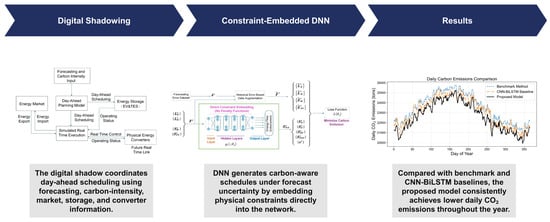
This paper proposes a DS-enabled deep learning framework for sustainable power-system scheduling under forecast uncertainty. The framework is designed to coordinate renewable generation, energy storage systems, and conventional energy-conversion devices within a carbon-aware smart-grid operation setting. The key idea is to embed hard physical constraints into the neural architecture so that feasibility is guaranteed for every inference, while optimizing a carbon-first objective that internalizes both scheduled and imbalance-driven emissions. The framework refines the device taxonomy into three categories. Memory devices such as EVs and TES are governed by SOC dynamics that couple decisions across time and provide storage flexibility for renewable integration. Non-memory fast devices, including transformers and CHP units, can change output instantaneously and are therefore constrained mainly by capacity limits. Non-memory ramp-limited devices, such as boilers or other slow thermal units, additionally face inter-temporal ramping constraints that limit the rate of change between consecutive time steps. Each device category is handled through a tailored transformation: fast devices are processed by direct normalization and scaling within admissible ranges; ramp-limited devices are adjusted using a ramp projection layer that enforces both upward and downward limits; and memory devices are mapped through a structured projection pipeline that includes net-zero energy alignment, instantaneous bounding, and SOC trajectory enforcement. Together, these procedures form a feasibility-by-design decoder that ensures all neural outputs comply with physical laws while remaining fully differentiable for end-to-end training.

Carbon optimization is handled by a carbon-intensity objective that aggregates (i) scheduled emissions computed with time-varying marginal carbon intensity and (ii) imbalance emissions priced with an “emergency” carbon factor to reflect the higher-carbon mix typically used to cover forecast deviations. This explicitly steers the scheduler toward profiles that not only plan low-carbon supply but also reduce exposure to carbon-heavy real-time corrections. Uncertainty is modeled statistically by sampling historical forecast-error patterns to build augmented training scenarios; the network thus learns a policy that is carbon-efficient in expectation without assuming parametric error distributions.

Extensive case studies on U.K. data show that the framework reduces annual CO₂ emissions by ∼3.96% relative to a forecast-driven baseline, with larger gains in high-demand winter months, while producing plans that are feasible at first pass and therefore directly executable by the DS. Ablations confirm that feasibility-by-design stabilizes training and removes the need for costly constraint repairs, and that the carbon-aware objective materially changes dispatch away from solutions that would be cost-attractive but emissions-intensive under imbalance.

Contributions

• A sustainable power-system scheduling framework is developed to coordinate renewable generation, grid imports, CHP units, boilers, EVs, and TES under forecast uncertainty.
• A feasibility-by-design neural decoder is proposed to embed hard operational constraints of energy storage devices, fast-response units, and ramp-limited devices directly into the learning architecture.
• A carbon-first objective is formulated to reduce both scheduled emissions and imbalance-driven emissions, supporting low-carbon smart-grid operation and renewable integration.
• A digital-shadow-assisted training and execution loop is established to learn from historical forecast-error patterns and generate feasible day-ahead schedules without post-hoc repair.
• An empirical evaluation based on U.K. data demonstrates consistent emission reductions, full schedule feasibility, and improved robustness compared with representative benchmark methods.

The remainder of this paper is organized as follows. Section 2 describes the system model and mathematical formulation of the integrated energy system, together with the proposed device taxonomy and constraint-embedding mechanism. Section 3 presents the proposed deep-learning-based scheduling framework, including the network architecture, uncertainty handling through data augmentation, and digital-shadow-assisted scheduling and adaptation. Section 4 provides the case studies and discusses the experimental results from multiple temporal perspectives, together with benchmark comparisons. Section 5 concludes the paper and discusses future research directions.

2. System Model

This section introduces the physical structure and mathematical formulation of the integrated energy system (IES) considered in this study. From the perspective of sustainable power systems, the IES represents a smart multi-energy infrastructure that coordinates renewable generation, conventional energy-conversion devices, and distributed energy storage to satisfy electricity and heat demands with reduced carbon emissions. The system couples multiple energy carriers, including electricity, heat, and distributed storage, following the foundational principles of the energy hub concept [21,22]. Understanding these interactions is essential before defining the scheduling problem and associated constraints.

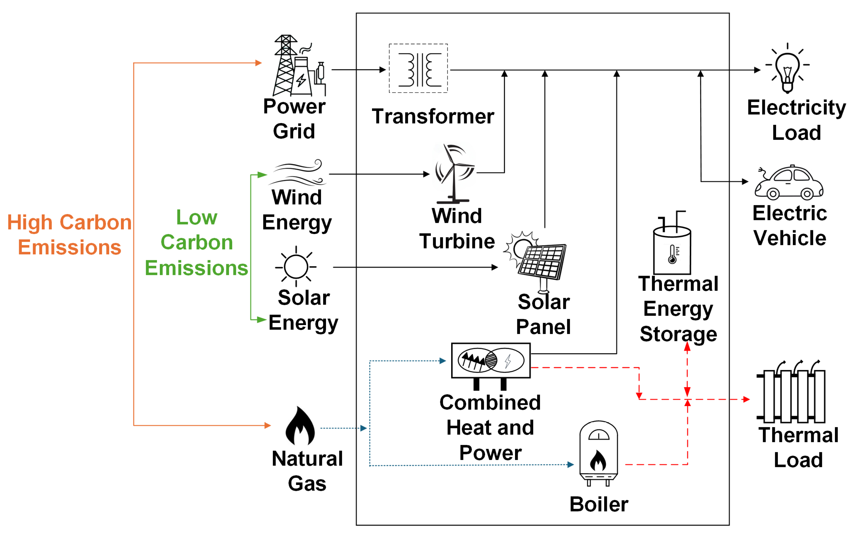
Figure 1 presents the overall architecture of the IES. Renewable energy resources such as wind turbines and photovoltaic arrays supply low-carbon electricity, while non-renewable units—including transformers, CHP systems, and boilers—provide supplemental electrical and thermal energy [23]. Distributed storage units, namely EVs and TES, introduce inter-temporal flexibility through their SOC dynamics [24,25]. The system must continuously satisfy both electrical demand $L_{\mathrm{elec}}^t$ and thermal demand $L_{\mathrm{heat}}^t$, which vary across the scheduling horizon. Compared with non-memory units (e.g., transformers, CHP), memory devices (EVs, TES) exhibit temporal coupling via SOC evolution, and boilers additionally experience ramp constraints, making coordinated scheduling essential.

2.1. Problem Formulation

We consider a day-ahead scheduling problem for an IES that couples electricity, heat, and distributed flexibility such as EVs and TES. The scheduling horizon is 24 h with hourly resolution, indexed by $t=1,\dots ,T$.

2.1.1. Decision Variables

At each time slot t, the scheduler determines:

• $S_E^t$: transformer electricity import (MW),
• $S_G^t$: CHP natural gas input (MW),
• $S_B^t$: boiler natural gas input (MW),
• $P_{\mathrm{EV}}^{\mathrm{ch},t},P_{\mathrm{EV}}^{\mathrm{dis},t}$: EV charging/discharging power (MW),
• $P_{\mathrm{TES}}^{\mathrm{ch},t},P_{\mathrm{TES}}^{\mathrm{dis},t}$: TES charging/discharging power (MW),
• $P_{\mathrm{PV},\mathrm{curt}}^t$: curtailed PV power caused by renewable overproduction, inverter clipping, or limited local absorption capacity (MW).

Dispatch factors $v_{\mathrm{CHP}}^t,v_B^t\in [0,1]$ allocate CHP and boiler inputs to electricity or heat outputs.

System Balance

At each t, the IES must satisfy both electrical and thermal demand, following standard multi-carrier energy balance principles [26]:

$$L_{\mathrm{elec}}^t=S_E^t+v_{\mathrm{CHP}}^t{S}_G^t+P_{\mathrm{EV}}^{\mathrm{dis},t}-P_{\mathrm{EV}}^{\mathrm{ch},t}+S_W^t+S_{\mathrm{PV}}^t-P_{\mathrm{PV},\mathrm{curt}}^t,$$

(1)

$$L_{\mathrm{heat}}^t=(1-v_{\mathrm{CHP}}^t)S_G^t+v_B^t{S}_B^t+P_{\mathrm{TES}}^{\mathrm{dis},t}-P_{\mathrm{TES}}^{\mathrm{ch},t}.$$

(2)

Here, $L_{\mathrm{elec}}^t$ and $L_{\mathrm{heat}}^t$ denote the predicted electricity and heat demands, while $S_W^t$ and $S_{\mathrm{PV}}^t$ denote the available wind and PV generation, respectively. The term $P_{\mathrm{PV},\mathrm{curt}}^t$ represents PV power that is curtailed when available PV generation exceeds the combined absorption capacity of local demand, storage devices, and admissible grid export or inverter limits. The utilized PV power is therefore defined as

$$\begin{array}{c}\hfill P_{\mathrm{PV},\mathrm{use}}^t=S_{\mathrm{PV}}^t-P_{\mathrm{PV},\mathrm{curt}}^t.\end{array}$$

(3)

The curtailment variable is bounded by

$$\begin{array}{c}\hfill 0\le P_{\mathrm{PV},\mathrm{curt}}^t\le S_{\mathrm{PV}}^t, \forall t.\end{array}$$

(4)

This formulation provides a physically admissible mechanism for handling severe midday PV overproduction. When EVs and TES are unavailable or fully charged and grid export or inverter capacity is insufficient, the surplus PV power is curtailed rather than being forced into infeasible charging, storage, or export decisions.

In this study, PV generation is represented at the scheduling level by the forecasted available PV power $S_{\mathrm{PV}}^t$ rather than by a detailed module-level electro-thermal model. When the PV profile is derived from irradiance data, a constant performance ratio assumption is adopted:

$$\begin{array}{c}\hfill S_{\mathrm{PV}}^t=P{R}_{\mathrm{PV}}{P}_{\mathrm{PV}}^{\mathrm{rated}}{\displaystyle \frac{G^t}{G^{\mathrm{STC}}}},\end{array}$$

(5)

where $P{R}_{\mathrm{PV}}$ is the constant PV performance ratio, $P_{\mathrm{PV}}^{\mathrm{rated}}$ is the rated PV capacity, $G^t$ is the incident solar irradiance at time t, and $G^{\mathrm{STC}}$ is the irradiance under standard test conditions. Temperature-dependent PV efficiency variation is not explicitly modeled in the present scheduling formulation. Instead, its aggregate effect is assumed to be reflected in the historical or forecasted PV generation data and in the PV forecast-error database used by the DS. This assumption is consistent with the system-level focus of this work, while component-level PV temperature modeling is left for future digital-shadow extensions.

Device Constraints

We refine the device taxonomy into three classes:

(i) Non-memory fast devices (transformer, CHP).

These devices do not involve inter-temporal states, so their decisions are bounded only by instantaneous capacities:

$$\begin{array}{cc}\hfill 0& \le S_E^t\le S_{\mathrm{TF}}^{\max }, \hfill \end{array}$$

(6)

$$\begin{array}{cc}\hfill 0& \le v_{\mathrm{CHP}}^t{S}_G^t\le S_{\mathrm{CHP}}^{\max }.\hfill \end{array}$$

(7)

Equation (6) ensures transformer imports do not exceed rated capacity. Equation (7) constrains the gas input allocated to the CHP. The corresponding CHP outputs are divided between electricity and heat according to $v_{\mathrm{CHP}}^t$.

(ii) Non-memory ramp-limited devices (boiler).

The boiler consumes natural gas $S_B^t$ to produce thermal energy. A dispatch factor $v_B^t\in [0,1]$ controls the effective output level. The operating constraints incorporate ramping limits to reflect thermal inertia [27]:

$$\begin{array}{cc}\hfill 0& \le v_B^t{S}_B^t\le S_B^{\max }, \hfill \end{array}$$

(8)

$$\begin{array}{cc}\hfill -R_B^{\mathrm{down}} & \le v_B^t{S}_B^t-v_B^{t-1}{S}_B^{t-1}\le R_B^{\mathrm{up}}, t>1,\hfill \end{array}$$

(9)

where $S_B^{\max }$ is the boiler capacity, and $R_B^{\mathrm{up}}$ and $R_B^{\mathrm{down}}$ denote the maximum upward and downward ramp rates.

(iii) Memory devices (EVs, TES).

Unlike non-memory units whose operating decisions affect only the current time slot, memory-type devices such as EVs and TES possess internal energy states that evolve over time. Their charging and discharging behaviors must therefore satisfy two sets of constraints: (i) instantaneous power limits, which prevent infeasible charging or discharging rates within a single period, and (ii) inter-temporal SOC dynamics, which ensure physically valid energy accumulation and depletion trajectories across the scheduling horizon.

(a) Instantaneous power limits.

At any time slot t, the charging or discharging power of each memory-type device must remain within its rated operating range [28].

(i) Contracted EV storage resource. It should be clarified that the EV subsystem considered in this study does not represent ordinary private EVs that follow daily commuting patterns. The mobility-related charging demand of ordinary EV users is treated as part of the electrical load $L_{\mathrm{elec}}^t$. In contrast, the EV variable in the proposed IES model represents a contracted EV storage resource that is connected to the charging node during a pre-agreed scheduling window and can be dispatched by the IES operator within that contractual period. To represent this assumption, a contractual availability indicator $A_{\mathrm{EV}}^{\mathrm{con},t}\in \{0,1\}$ is introduced, where $A_{\mathrm{EV}}^{\mathrm{con},t}=1$ indicates that the contracted EV resource is connected and dispatchable, while $A_{\mathrm{EV}}^{\mathrm{con},t}=0$ indicates that it is unavailable. The instantaneous EV charging and discharging power therefore satisfies

$$\begin{array}{c}\hfill -A_{\mathrm{EV}}^{\mathrm{con},t}{P}_{\mathrm{EV}}^{\max ,\mathrm{Ch}}\le P_{\mathrm{EV}}^t\le A_{\mathrm{EV}}^{\mathrm{con},t}{P}_{\mathrm{EV}}^{\max ,\mathrm{Dis}},\end{array}$$

(10)

where $P_{\mathrm{EV}}^t>0$ indicates discharging to the IES, and $P_{\mathrm{EV}}^t<0$ denotes charging from the IES. In the base-case contract considered in this study, the contracted EV resource remains connected throughout the 24-h scheduling horizon, i.e., $A_{\mathrm{EV}}^{\mathrm{con},t}=1$ for all $t=1,\dots ,T$. This contractual setting differs from a residential commuting EV profile and prevents misinterpreting the EV subsystem as unconstrained private mobility.

(ii) TES. For the thermal storage system, a similar bound is imposed:

$$\begin{array}{c}\hfill -P_{\mathrm{TES}}^{\max ,\mathrm{Ch}}\le P_{\mathrm{TES}}^t\le P_{\mathrm{TES}}^{\max ,\mathrm{Dis}},\end{array}$$

(11)

where $P_{\mathrm{TES}}^t>0$ corresponds to heat discharge to the IES, and $P_{\mathrm{TES}}^t<0$ represents heat charging or accumulation.

(b) SOC dynamics and trajectory constraints.

Beyond instantaneous power limits, the energy content of each memory-type device must evolve consistently with its charging and discharging operations. The SOC reflects the cumulative energy stored within the device and evolves across time according to charging/discharging decisions and associated efficiency factors. Separate formulations are provided for EVs and TES to capture their distinct physical behaviors [29].

(i) EV. The aggregated SOC of the EV fleet evolves according to

$$\begin{array}{c}\hfill SO{C}_{\mathrm{EV}}^t=SO{C}_{\mathrm{EV}}^{t-1}+{\eta }_{\mathrm{EV}}^{\mathrm{ch}}{P}_{\mathrm{EV}}^{\mathrm{ch},t}\Delta t-{\displaystyle \frac{1}{{\eta }_{\mathrm{EV}}^{\mathrm{dis}}}}{P}_{\mathrm{EV}}^{\mathrm{dis},t}\Delta t,\end{array}$$

(12)

where ${\eta }_{\mathrm{EV}}^{\mathrm{ch}}$ and ${\eta }_{\mathrm{EV}}^{\mathrm{dis}}$ denote the charging and discharging efficiencies, while $\Delta t$ represents the time-step duration. The SOC must remain within operational bounds:

$$\begin{array}{c}\hfill SO{C}_{\mathrm{EV}}^{\min }\le SO{C}_{\mathrm{EV}}^t\le SO{C}_{\mathrm{EV}}^{\max }, \forall t,\end{array}$$

(13)

where $SO{C}_{\mathrm{EV}}^{\min }$ and $SO{C}_{\mathrm{EV}}^{\max }$ denote minimum and maximum allowable storage levels. To maintain daily energy neutrality, a terminal consistency constraint is imposed:

$$\begin{array}{c}\hfill SO{C}_{\mathrm{EV}}^T=SO{C}_{\mathrm{EV}}^0.\end{array}$$

(14)

Here, the superscript T denotes the final time step of the scheduling horizon, while the superscript 0 represents the initial condition.

(ii) TES. The SOC of the TES unit evolves as typical thermal inertia models [30]:

$$\begin{array}{c}\hfill SO{C}_{\mathrm{TES}}^t=SO{C}_{\mathrm{TES}}^{t-1}+{\eta }_{\mathrm{TES}}^{\mathrm{ch}}{P}_{\mathrm{TES}}^{\mathrm{ch},t}\Delta t-{\displaystyle \frac{1}{{\eta }_{\mathrm{TES}}^{\mathrm{dis}}}}{P}_{\mathrm{TES}}^{\mathrm{dis},t}\Delta t,\end{array}$$

(15)

where $SO{C}_{\mathrm{TES}}^t$ denotes the state of charge of the TES at time step t, $P_{\mathrm{TES}}^{\mathrm{ch},t}$ and $P_{\mathrm{TES}}^{\mathrm{dis},t}$ represent the charging and discharging power, respectively, and ${\eta }_{\mathrm{TES}}^{\mathrm{ch}}$ and ${\eta }_{\mathrm{TES}}^{\mathrm{dis}}$ denote the corresponding charging and discharging efficiencies. $\Delta t$ is the duration of each time step. The SOC must remain within feasible bounds:

$$\begin{array}{c}\hfill SO{C}_{\mathrm{TES}}^{\min }\le SO{C}_{\mathrm{TES}}^t\le SO{C}_{\mathrm{TES}}^{\max }, \forall t,\end{array}$$

(16)

and a terminal neutrality condition ensures net-zero change over the horizon:

$$\begin{array}{c}\hfill SO{C}_{\mathrm{TES}}^T=SO{C}_{\mathrm{TES}}^0.\end{array}$$

(17)

Carbon Intensity Formulation

The overall carbon performance of the proposed scheduling framework is quantified through an aggregate carbon intensity index ${\mathrm{CI}}_{\mathrm{all}}$, which combines the scheduled emissions from day-ahead dispatch ${\mathrm{CI}}_{\mathrm{schedule}}$ and the additional emissions caused by real-time imbalances ${\mathrm{CI}}_{\mathrm{extra}}$.

$$\begin{array}{c}\hfill {\mathrm{CI}}_{\mathrm{all}}= {\mathrm{CI}}_{\mathrm{schedule}}+{\mathrm{CI}}_{\mathrm{extra}}. \end{array}$$

(18)

(a) Scheduled carbon intensity. The scheduled component ${\mathrm{CI}}_{\mathrm{schedule}}$ represents the emissions directly resulting from the planned day-ahead operation of energy-converting devices. At each time step, the scheduled emission rate is determined by the instantaneous carbon intensity of the energy sources used, reflecting the varying grid mix [31]. For the integrated energy system considered, the carbon contribution at time t is expressed as

$$\begin{array}{c}\hfill E_{\mathrm{schedule}}^t=\left(S_E^t+P_{\mathrm{CHP}}^t+P_{\mathrm{Boiler}}^t-P_{\mathrm{EV}}^t-P_{\mathrm{TES}}^t\right) {\mathrm{CI}}^t,\end{array}$$

(19)

where $S_E^t$, $P_{\mathrm{CHP}}^t$, and $P_{\mathrm{Boiler}}^t$ denote the scheduled electrical or thermal power supplied by the transformer, CHP, and boiler. The terms $P_{\mathrm{EV}}^t$ and $P_{\mathrm{TES}}^t$ represent the net power absorbed by EV and TES subsystems. Positive values indicate energy delivery to the grid or demand side, whereas negative values indicate charging or storage. Renewable generation is assumed carbon-free; thus, only conventional energy conversion contributes to ${\mathrm{CI}}_{\mathrm{schedule}}$. ${\mathrm{CI}}^t$ denotes the time-varying carbon intensity at time step t, reflecting the emission factor of the energy supply mix.

(b) Extra carbon intensity. The second component, ${\mathrm{CI}}_{\mathrm{extra}}$, captures additional emissions caused by real-time deviations between forecasted and actual system states. When forecast errors occur, the instantaneous electrical and thermal balances become

$$\begin{array}{cc}\hfill \Delta E^t& =L_{\mathrm{elec}}^t-\left(S_E^t+P_{\mathrm{CHP},\mathrm{E}}^t+S_W^t+S_{\mathrm{PV}}^t+P_{\mathrm{EV}}^t\right),\hfill \\ \hfill \Delta H^t& =L_{\mathrm{heat}}^t-\left(P_{\mathrm{CHP},\mathrm{H}}^t+P_{\mathrm{Boiler}}^t+P_{\mathrm{TES}}^t\right),\hfill \end{array}$$

(20)

where $L_E^t$ and $L_H^t$ denote the instantaneous electricity and heat demand, and the remaining terms represent the actual energy supplied by each device. Any residual mismatch must be met by fast real-time balancing actions, typically involving higher-emission resources [32].

To reflect this, imbalance-induced emissions at time t are modeled as

$$\begin{array}{c}\hfill E_{\mathrm{extra}}^t=\left(|\Delta E^t|+|\Delta H^t|\right) {\mathrm{CI}}_{\mathrm{emer}}^t,\end{array}$$

(21)

where ${\mathrm{CI}}_{\mathrm{emer}}^t$ denotes the market-determined real-time extra carbon-intensity cost associated with emergency balancing actions at time t. This term is not introduced as an arbitrary penalty coefficient. Instead, it is used to represent the carbon impact of real-time corrective actions required to compensate forecast-induced mismatches. This formulation follows the same operational logic as previous DT-based IES scheduling studies, where the total operating cost is decomposed into a day-ahead scheduled component and a real-time extra correction component caused by forecast errors. In the economic formulation, this extra component is determined by real-time electricity and gas market prices. In the present work, the same idea is extended to the carbon-emission domain: ${\mathrm{CI}}_{\mathrm{emer}}^t$ plays the role of a real-time extra carbon-intensity signal for imbalance-driven emissions.

When time-resolved market-based real-time extra carbon-intensity data are available, ${\mathrm{CI}}_{\mathrm{emer}}^t$ can be directly used in Equation (21). In the present case study, an aggregate market-informed value, denoted by ${\mathrm{CI}}_{\mathrm{emer}}$, is used:

$$\begin{array}{c}\hfill {\mathrm{CI}}_{\mathrm{emer}}={\displaystyle \frac{1}{T_{\mathrm{train}}}}\sum _{t\in {\mathcal{T}}_{\mathrm{train}}}{\mathrm{CI}}_{\mathrm{RT},\mathrm{extra}}^t,\end{array}$$

(22)

where ${\mathrm{CI}}_{\mathrm{RT},\mathrm{extra}}^t$ denotes the real-time extra carbon-intensity cost observed or estimated from balancing-market operation. Therefore, the selection of ${\mathrm{CI}}_{\mathrm{emer}}$ is market-informed rather than manually tuned. Since the real-time extra carbon-intensity signal may vary with balancing-market conditions, reserve dispatch, and system stress, a more comprehensive sensitivity analysis of ${\mathrm{CI}}_{\mathrm{emer}}$ will be included in future work together with real-time market data with higher temporal resolution.

(c) Total carbon emission objective. The total carbon-related cost is defined as

$$\begin{array}{c}\hfill E_{\mathrm{total}}^t=E_{\mathrm{schedule}}^t+E_{\mathrm{extra}}^t,\end{array}$$

(23)

and the day-ahead scheduling objective minimizes the cumulative emissions ${\sum }_{t=1}^T{E}_{\mathrm{total}}^t$ across the planning horizon [33]. This formulation ensures that both scheduled operations and forecast-induced imbalances are reflected in the carbon objective, encouraging schedules that minimize ${\mathrm{CI}}_{\mathrm{all}}$ by favoring low-carbon mixes and reducing reliance on emergency balancing resources.

Optimization Problem

The day-ahead scheduling problem aims to determine the optimal power and energy trajectories of all devices that minimize total carbon emissions while ensuring physical feasibility and operational balance across the 24-h horizon. The problem is formulated as

$$\begin{array}{cc}\hfill \underset{{\{S_E^t, S_G^t, S_B^t, P_{\mathrm{EV}}^t, P_{\mathrm{TES}}^t, P_{\mathrm{PV},\mathrm{curt}}^t\}}_{t=1}^T}{\min } & {\displaystyle \sum _{t=1}^T}{E}_{\mathrm{total}}^t\hfill \\ \hfill \mathrm{s}.\mathrm{t}. & (\mathrm{Equations} \left(1\right) \mathrm{and} (2\left)\right),\hfill \\ \hfill & (\mathrm{Equations} \left(6\right) \mathrm{and} (7\left)\right),\hfill \\ \hfill & (\mathrm{Equations} \left(8\right) \mathrm{and} (9\left)\right),\hfill \\ \hfill & (\mathrm{Equations} (10), (12)–(14\left)\right),\hfill \\ \hfill & (\mathrm{Equations} (11), (15)–(17\left)\right),\hfill \\ \hfill & (\mathrm{Equations} (18)–(23\left)\right),\hfill \\ \hfill & (\mathrm{Equations} \left(3\right) \mathrm{and} (4\left)\right).\hfill \end{array}$$

(24)

This formulation captures all device-level operational constraints, system-level balance requirements, and carbon-based objectives, ensuring that the resulting schedule is both physically feasible and carbon-aware.

The above formulation captures detailed physical and operational constraints of the IES, including capacity limits, ramp-rate restrictions, and inter-temporal SOC dynamics. However, directly incorporating these constraints into learning-based scheduling models remains challenging. Conventional approaches typically rely on penalty terms or post-hoc correction mechanisms, which do not guarantee feasibility and may lead to constraint violations during inference.

To address this issue, it is necessary to explicitly embed these constraints into the model structure. This motivates the constraint embedding mechanism introduced in Section 2.2, which ensures that all generated schedules satisfy physical constraints by construction.

2.2. Device Taxonomy and Constraint Embedding

To guarantee feasibility of the neural network outputs at inference, a feasibility-by-design decoder is developed to embed the physical constraints of Section 2.1 directly into the forward pass. This approach aligns with the emerging paradigm of constrained deep learning, where optimization requirements are integrated into the neural architecture rather than treated as soft penalties [17,18]. Each device category—non-memory fast, non-memory ramp-limited, and memory-type—is associated with a specific transformation rule that enforces capacity, inter-temporal, and ramping constraints by construction.

From a methodological perspective, the proposed decoder differs from generic constrained learning layers in both formulation and operation. Many existing end-to-end constrained learning methods introduce an optimization layer that projects a neural prediction onto a feasible set by solving a constrained problem during the forward pass. Such approaches are powerful and general, but the feasibility set is usually treated as a monolithic constraint region. In contrast, the proposed decoder decomposes the feasible scheduling set according to the physical taxonomy of IES devices. Let $\mathcal{F}$ denote the feasible set of all device schedules. Instead of learning an unconstrained mapping $g_{\theta }\left(F\right)$ and subsequently repairing it through a separate projection ${\mathrm{\Pi }}_{\mathcal{F}}(·)$, the proposed framework constructs a structured mapping

$$\begin{array}{c}\hfill g_{\theta }\left(F\right)={\mathcal{D}}_{\mathrm{mem}}\circ {\mathcal{D}}_{\mathrm{ramp}}\circ {\mathcal{D}}_{\mathrm{fast}}\left(h_{\theta }\left(F\right)\right),\end{array}$$

(25)

where $h_{\theta }(·)$ is the unconstrained neural representation, and ${\mathcal{D}}_{\mathrm{fast}}$, ${\mathcal{D}}_{\mathrm{ramp}}$, and ${\mathcal{D}}_{\mathrm{mem}}$ are device-specific constraint mappings for instantaneous-capacity devices, ramp-limited devices, and SOC-coupled memory devices, respectively. Each mapping is designed so that its output belongs to the corresponding physical feasible subset. Therefore, the final schedule satisfies

$$\begin{array}{c}\hfill g_{\theta }\left(F\right)\in \mathcal{F}, \forall F,\end{array}$$

(26)

by construction.

This formulation advances constrained deep learning for IES scheduling in three aspects. First, feasibility is embedded before schedule evaluation rather than added as a penalty after violation occurs. Second, the constraint treatment is device-structured: different physical mechanisms, such as capacity saturation, ramp-rate continuity, and SOC accumulation, are enforced by different analytical transformations. Third, the decoder avoids repeatedly solving a full constrained optimization problem at inference, making it suitable for repeated day-ahead scheduling and digital-shadow-assisted scenario evaluation. In this sense, the proposed feasibility-by-design philosophy provides an interpretable and computationally lightweight alternative to generic optimization-layer-based constraint enforcement for heterogeneous IES scheduling.

2.2.1. Non-Memory Fast Devices (Transformer, CHP)

For non-memory fast devices, such as the transformer and CHP unit, only instantaneous capacity limits are relevant (Equations (6) and (7)). These limits are embedded through direct normalization and scaling: the neural network output corresponding to each device is first mapped to $[0,1]$ via a bounded activation function and then scaled by the rated capacity. This ensures that every predicted dispatch point lies within the admissible operating range without post-processing.

In the neural decoder, the outputs corresponding to non-memory fast devices are processed through smooth bounded transformations to guarantee compliance with their instantaneous capacity limits. Two representative devices in this category are the transformer and the CHP unit.

• Transformer (electricity import).
  The raw neural output for transformer power, denoted $S_E^{\mathrm{raw},t}$, is normalized into the unit interval $[0,1]$ using a sigmoid activation:

  $${\tilde{S}}_E^t =\sigma \left(S_E^{\mathrm{raw},t}\right)={\displaystyle \frac{1}{1+e^{-S_E^{\mathrm{raw},t}}}}.$$

  (27)

  The normalized value is then scaled by the transformer’s rated capacity:

  $$S_E^t ={\tilde{S}}_E^t S_{\mathrm{TF}}^{\max }.$$

  (28)

  ensuring $0\le S_E^t\le S_{\mathrm{TF}}^{\max }$ at every time step, consistent with Equation (6).
• CHP unit (gas input and dispatch factor).
  For the CHP system, two variables must remain within feasible ranges: the normalized dispatch factor $v_{\mathrm{CHP}}^t\in [0,1]$ and the gas input $S_G^t$ bounded by its rated limit. The raw network outputs $v_{\mathrm{CHP}}^{\mathrm{raw},t}$ and $S_G^{\mathrm{raw},t}$ are mapped via sigmoid activations:

  $${\tilde{v}}_{\mathrm{CHP}}^t =\sigma \left(v_{\mathrm{CHP}}^{\mathrm{raw},t}\right),$$

  (29)

  $${\tilde{S}}_G^t =\sigma \left(S_G^{\mathrm{raw},t}\right).$$

  (30)

  The feasible values are then obtained by scaling:

  $$v_{\mathrm{CHP}}^t ={\tilde{v}}_{\mathrm{CHP}}^t,$$

  (31)

  $$S_G^t ={\tilde{S}}_G^t S_{\mathrm{CHP}}^{\max }.$$

  (32)

  ensuring that $0\le v_{\mathrm{CHP}}^t{S}_G^t\le S_{\mathrm{CHP}}^{\max }$, consistent with Equation (7).

Both the sigmoid activation and the scaling operations are smooth and differentiable, allowing gradient information to propagate through these mappings during training. The decoder thus enforces feasibility of transformer and CHP outputs by design, ensuring physically valid trajectories without post-hoc projection or penalty terms.

2.2.2. Non-Memory Ramp-Limited Devices (Boilers)

Boilers convert natural gas to thermal output, controlled by a dispatch factor $v_B^t\in [0,1]$. The instantaneous and ramping constraints are

$$0 \le v_B^t{S}_B^t\le S_B^{\max },$$

(33)

$$-R_B^{\mathrm{down}} \le \left(v_B^t{S}_B^t\right)-\left(v_B^{t-1}{S}_B^{t-1}\right)\le R_B^{\mathrm{up}}.$$

(34)

To enforce these constraints within the neural network output, a two-stage transformation is used. First, a box projection maps raw predictions into the admissible instantaneous range:

$${\tilde{P}}_B^t=S_B^{\max }·\sigma \left(x^{\mathrm{raw},t}\right).$$

(35)

where $x^{\mathrm{raw},t}$ is the unconstrained network output at time t and $\sigma (·)$ denotes the sigmoid activation. This ensures ${\tilde{P}}_B^t\in [0,S_B^{\max }]$ for all t.

Second, the sequence ${\left\{{\tilde{P}}_B^t\right\}}_{t=1}^T$ is passed through a Ramp Projection Layer (RPL) to enforce compliance with inter-temporal ramp-rate constraints. The RPL is defined as a deterministic projection operator that maps an unconstrained trajectory to the nearest feasible trajectory under ramp-rate constraints. This layer functions as a computationally efficient proximal operator, projecting the initial guess onto the feasible polytope [34].

• Forward sweep (up-ramp limit).
  Starting from the initial output $P_B^0$, the adjusted sequence $U^t$ enforces that the increase between consecutive steps does not exceed the up-ramp limit $R_B^{\mathrm{up}}$:

  $$U^1=\min ({\tilde{P}}_B^1, P_B^0+R_B^{\mathrm{up}}),$$

  (36)

  $$U^t=\min ({\tilde{P}}_B^t, U^{t-1}+R_B^{\mathrm{up}}), t=2,\dots ,T.$$

  (37)
• Backward sweep (down-ramp limit).
  Beginning from $t=T$, the sequence enforces that decreases between steps do not exceed the down-ramp limit $R_B^{\mathrm{down}}$:

  $$V^T=U^T,$$

  (38)

  $$V^t=\max (U^t, V^{t+1}-R_B^{\mathrm{down}}), t=T-1,\dots ,1.$$

  (39)
• Final clipping.
  The ramp-limited sequence is then clipped to respect instantaneous bounds:

  $$\begin{array}{c}\hfill P_B^t=\max \left(0, \min (V^t, S_B^{\max })\right), t=1,\dots ,T.\end{array}$$

  (40)

This procedure produces a feasible trajectory $\left\{P_B^t\right\}$ that satisfies both instantaneous capacity and ramp constraints. The RPL operates in linear time with respect to the horizon length and uses only min and max operations, making it computationally efficient. Since these operators are piecewise differentiable, gradients propagate through the layer during training, ensuring compatibility with end-to-end learning.

2.2.3. Memory Devices (EVs, TES)

Memory devices such as EVs and TES evolve according to SOC dynamics, making their feasible operating set more complex. Let $P_m^t$ denote the net charging ($P_m^t<0$) or discharging ($P_m^t>0$) power of memory device $m\in \{\mathrm{EV},\mathrm{TES}\}$. The power limits are

$$\begin{array}{c}\hfill -P_m^{\max ,\mathrm{Ch}}\le P_m^t\le P_m^{\max ,\mathrm{Dis}}.\end{array}$$

(41)

Their SOC evolves as

$$\begin{array}{c}\hfill SO{C}_m^t=SO{C}_m^{t-1}+{\eta }_m^{\mathrm{ch}}{P}_m^{\mathrm{ch},t}\Delta t-{\displaystyle \frac{1}{{\eta }_m^{\mathrm{dis}}}}{P}_m^{\mathrm{dis},t}\Delta t,\end{array}$$

(42)

subject to bounds

$$\begin{array}{c}\hfill SO{C}_m^{\min }\le SO{C}_m^t\le SO{C}_m^{\max }, \forall t,\end{array}$$

(43)

and terminal neutrality

$$\begin{array}{c}\hfill SO{C}_m^T=SO{C}_m^0.\end{array}$$

(44)

To embed these constraints into the neural decoder, structured transformations are applied separately for EVs and TES. This reflects the philosophy of physics-informed deep learning, where governing equations are embedded into the model structure [35]. Each transformation consists of three sequential stages—net-zero alignment, instantaneous bounding, and SOC trajectory enforcement—ensuring that both instantaneous and inter-temporal constraints are satisfied by design.

(i)

EV

The aggregated EV subsystem stores electrical energy and must satisfy both power limits and SOC dynamics. The raw neural outputs are transformed as follows.

• Mean offset removal (net-zero alignment).
  The raw sequence ${\left\{y_{\mathrm{EV}}^t\right\}}_{t=1}^T$ is centered to ensure the terminal neutrality requirement:

  $$\begin{array}{c}\hfill {\tilde{y}}_{\mathrm{EV}}^t=y_{\mathrm{EV}}^t-{\displaystyle \frac{1}{T}}{\displaystyle \sum _{\tau =1}^T}{y}_{\mathrm{EV}}^{\tau }.\end{array}$$

  (45)

  This guarantees ${\sum }_{t=1}^T{\tilde{y}}_{\mathrm{EV}}^t=0$.
• Flow rate bounding (instantaneous feasibility).
  The centered outputs are mapped into the admissible charging/discharging range using a sigmoid mapping:

  $$\begin{array}{c}\hfill {\widehat{P}}_{\mathrm{EV}}^t=-A_{\mathrm{EV}}^{\mathrm{con},t}{P}_{\mathrm{EV}}^{\max ,\mathrm{Ch}}+\sigma \left({\tilde{y}}_{\mathrm{EV}}^t\right)A_{\mathrm{EV}}^{\mathrm{con},t}\left(P_{\mathrm{EV}}^{\max ,\mathrm{Ch}}+P_{\mathrm{EV}}^{\max ,\mathrm{Dis}}\right).\end{array}$$

  (46)
• SOC trajectory enforcement (inter-temporal feasibility).
  SOC evolves as

  $$\begin{array}{cc}\hfill SO{C}_{\mathrm{EV}}^t=& SO{C}_{\mathrm{EV}}^{t-1}+{\eta }_{\mathrm{EV}}^{\mathrm{ch}}\max ({\widehat{P}}_{\mathrm{EV}}^t,0)\Delta t\hfill \\ \hfill & -{\displaystyle \frac{1}{{\eta }_{\mathrm{EV}}^{\mathrm{dis}}}}\max (-{\widehat{P}}_{\mathrm{EV}}^t,0)\Delta t.\hfill \end{array}$$

  (47)

  If SOC violates its bounds, a uniform scaling factor ${\alpha }_{\mathrm{EV}}\in (0,1]$ is applied:

  $$\begin{array}{c}\hfill P_{\mathrm{EV}}^t={\alpha }_{\mathrm{EV}}{\widehat{P}}_{\mathrm{EV}}^t, \forall t.\end{array}$$

  (48)

  The scaling factor is chosen such that SOC exactly reaches its nearest bound, guaranteeing feasibility.

(ii)

TES

The TES subsystem follows the same three-stage transformation but incorporates thermal efficiencies:

• Mean offset removal (net-zero alignment).

  $$\begin{array}{c}\hfill {\tilde{y}}_{\mathrm{TES}}^t=y_{\mathrm{TES}}^t-{\displaystyle \frac{1}{T}}{\displaystyle \sum _{\tau =1}^T}{y}_{\mathrm{TES}}^{\tau }.\end{array}$$

  (49)
• Flow rate bounding (instantaneous feasibility).

  $$\begin{array}{c}\hfill {\widehat{P}}_{\mathrm{TES}}^t=-P_{\mathrm{TES}}^{\max ,\mathrm{Ch}}+\sigma \left({\tilde{y}}_{\mathrm{TES}}^t\right)\left(P_{\mathrm{TES}}^{\max ,\mathrm{Ch}}+P_{\mathrm{TES}}^{\max ,\mathrm{Dis}}\right).\end{array}$$

  (50)
• SOC trajectory enforcement.

  $$\begin{array}{cc}\hfill SO{C}_{\mathrm{TES}}^t=& SO{C}_{\mathrm{TES}}^{t-1}+{\eta }_{\mathrm{TES}}^{\mathrm{ch}}\max ({\widehat{P}}_{\mathrm{TES}}^t,0)\Delta t\hfill \\ \hfill & -{\displaystyle \frac{1}{{\eta }_{\mathrm{TES}}^{\mathrm{dis}}}}\max (-{\widehat{P}}_{\mathrm{TES}}^t,0)\Delta t.\hfill \end{array}$$

  (51)
  If SOC violates bounds, a scaling factor ${\alpha }_{\mathrm{TES}}$ is applied:

  $$\begin{array}{c}\hfill P_{\mathrm{TES}}^t={\alpha }_{\mathrm{TES}}{\widehat{P}}_{\mathrm{TES}}^t, \forall t.\end{array}$$

  (52)

All transformations consist of smooth (sigmoid, affine) or piecewise-linear (uniform scaling) mappings, making them compatible with gradient-based training. As a result, the decoder guarantees feasibility of EV and TES trajectories by design, without the need for post-hoc projection or penalty-based constraint handling.

2.2.4. PV Curtailment as a Bounded Residual Variable

PV curtailment is treated differently from the controllable device schedules. It is not introduced as an additional independent neural-network output, because the DNN is designed to generate dispatch trajectories for controllable IES devices, including the transformer, CHP unit, boiler, EV, and TES. Instead, PV curtailment is computed as a bounded residual variable during the digital-shadow-based balance evaluation.

After the feasibility-by-design decoder has generated physically feasible trajectories for all controllable devices, the DS evaluates whether the available renewable generation exceeds the admissible absorption capability of the IES. The residual surplus before PV curtailment can be expressed as

$$\begin{array}{c}\hfill P_{\mathrm{sur}}^t=S_W^t+S_{\mathrm{PV}}^t+S_E^t+v_{\mathrm{CHP}}^t{S}_G^t+P_{\mathrm{EV}}^{\mathrm{dis},t}-P_{\mathrm{EV}}^{\mathrm{ch},t}-L_{\mathrm{elec}}^t.\end{array}$$

(53)

If explicit grid export is not considered, the admissible export capacity is set to zero. More generally, let $P_{\exp }^{\max }$ denote the export or inverter headroom available for surplus electricity. The PV curtailment residual is then computed as

$$\begin{array}{c}\hfill P_{\mathrm{PV},\mathrm{curt}}^t=\min \left[S_{\mathrm{PV}}^t,\max \left(0, P_{\mathrm{sur}}^t-P_{\exp }^{\max }\right)\right].\end{array}$$

(54)

This operation guarantees $0\le P_{\mathrm{PV},\mathrm{curt}}^t\le S_{\mathrm{PV}}^t$ and therefore prevents physically impossible use of surplus PV generation. In the present case study, explicit electricity export is not modeled, so $P_{\exp }^{\max }=0$. Consequently, when local demand, EV charging, TES operation, and other admissible absorption paths cannot accommodate available PV generation, the remaining PV surplus is clipped through $P_{\mathrm{PV},\mathrm{curt}}^t$. This residual treatment preserves the original neural output dimension while structurally preventing the decoder from relying on unavailable storage or export capacity during severe midday overproduction.

2.2.5. Concatenation of Constrained Outputs

After processing non-memory fast devices, non-memory ramp-limited devices, and memory devices separately, their feasible outputs are concatenated into a single scheduling vector. This final vector is guaranteed to satisfy all physical and operational constraints at each time step. By embedding these constraint-enforcing transformations directly into the neural network forward pass, the architecture intrinsically produces feasible schedules without the need for penalty-based corrections or post-hoc repair.

2.3. Digital Shadowing Integration

The DS serves as a data-informed virtual representation of the physical IES, supporting forecasting, day-ahead scheduling, and operational analysis. In contrast to a fully bidirectional Digital Twin, the DS considered in this work does not directly actuate physical devices or claim autonomous closed-loop control. Instead, it mirrors the physical system through forecasted operating conditions, historical forecast-error patterns, and periodically updated device-state information. This one-way data-to-model mapping allows forecast information to be translated into feasible scheduling strategies, while enabling post-scheduling evaluation of system feasibility and carbon performance under uncertainty.

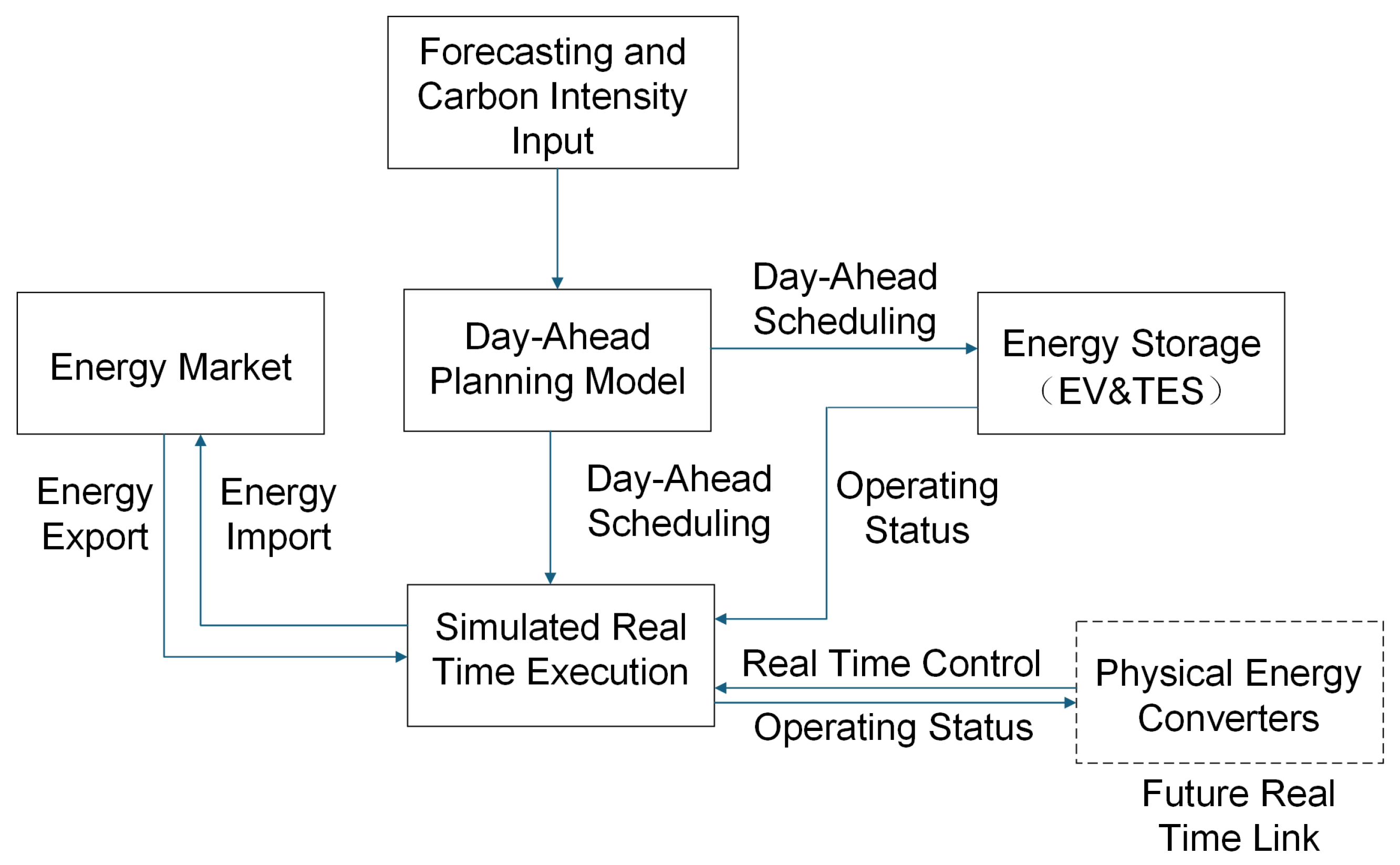
The DS framework, illustrated in Figure 2, is implemented at the system scheduling level. It receives day-ahead information on loads and renewable outputs,

$$\begin{array}{c}\hfill F^t=\{L_{\mathrm{elec}}^t, L_{\mathrm{heat}}^t, S_W^t, S_{\mathrm{PV}}^t\},\end{array}$$

(55)

where $L_{\mathrm{elec}}^t$ and $L_{\mathrm{heat}}^t$ denote the predicted electrical and thermal demands, while $S_W^t$ and $S_{\mathrm{PV}}^t$ denote the forecasted wind and photovoltaic generation available to the IES scheduler.

It should be clarified that the DS considered in this study is a scheduling-level digital shadow of the integrated energy system rather than a component-level physical digital shadow of each renewable device. In particular, $S_{PV}^t$ represents the forecasted AC-side PV power used for scheduling and uncertainty analysis. The present model does not dynamically synchronize internal PV module states such as cell temperature, soiling level, degradation state, or inverter operating point. These device-level effects are assumed to be reflected implicitly in the measured or forecasted PV generation profile and in the historical PV forecast-error database. Therefore, the role of the DS is to organize forecasted PV power, historical PV error patterns, load information, carbon-intensity signals, and device states into a unified virtual scheduling environment, rather than to provide a detailed electro-thermal digital shadow of the PV array itself.

These scheduling-level data streams serve as inputs to two complementary DS modules: the day-ahead scheduler and the real-time supervisory assessment module.

In the day-ahead stage, the DS generates an optimized dispatch plan for all devices, establishing baseline trajectories for both memory and non-memory units. The scheduled SOC paths of EVs and TES ensure future feasibility, while non-memory dispatch levels coordinate energy supply to anticipated demand.

In real-time operation, actual conditions typically deviate from forecasts. The DS supervises corrective actions by adjusting non-memory devices (e.g., transformers, CHP units) to compensate for deviations, while memory devices such as EVs and TES track their pre-scheduled SOC trajectories to preserve inter-temporal feasibility. Through this coordination, the DS balances fast-response flexibility with long-horizon stability, ensuring reliable operation under uncertainty.

An important feature of the DS is its closed-loop learning mechanism. Forecast errors observed during real-time execution are fed back into the forecasting module, improving prediction accuracy over time. This feedback loop enhances the robustness of subsequent scheduling cycles, enabling the DS to continually adapt to changes in load patterns, renewable variability, and operational conditions.

3. Proposed Deep Learning-Based Scheduling Method

3.1. Method Overview

The objective of the proposed method is to generate a feasible day-ahead schedule that minimizes total carbon emissions across the scheduling horizon while supporting sustainable power-system operation. The schedule includes multiple types of decision variables, such as energy exchanges with the external grid, charging and discharging decisions for energy storage devices (EVs and TES), and dispatch factors for non-memory units such as CHP systems and boilers. By jointly optimizing these decisions, the framework coordinates renewable integration, non-renewable generation, storage flexibility, and smart-grid-level digital control to satisfy both electricity and heat demands in a low-carbon and operationally feasible manner.

To capture the nonlinear mapping from forecasted conditions to device-level schedules, a deep neural network (DNN) is employed [36]. The DNN takes as input the day-ahead forecasts of electrical load, thermal load, and renewable generation, and outputs a complete dispatch plan over the 24-h horizon. Although advanced temporal architectures such as RNNs or Transformers could model inter-temporal dependencies explicitly, a fully connected feed-forward architecture is preferred due to its simplicity, scalability, and—most critically—its compatibility with constraint embedding. The feasibility-by-design decoder introduced in Section 2.2 integrates physical constraints directly into the forward pass, a task that is substantially easier to implement within a feed-forward structure.

Forecast uncertainty is addressed through data augmentation. Historical forecast error vectors are stored in a database, and each training sample is perturbed by drawing an error realization ${\delta }_t$. The resulting augmented scenario, ${\tilde{F}}_t=F_t+{\delta }_t$, exposes the DNN to a wide range of plausible realizations and encourages learning of robust scheduling policies that perform well in expectation. This reduces the reliance on high-carbon emergency balancing actions during real-time operation.

The entire framework is trained to minimize an expected carbon-emission objective. Unlike cost-centric formulations that only indirectly incentivize decarbonization, the proposed carbon-first objective directly aggregates scheduled emissions and imbalance-induced emissions, weighted by appropriate carbon intensity factors. By learning under this objective, the DNN generates feasible schedules that explicitly support decarbonization goals.

3.2. Neural Network Architecture

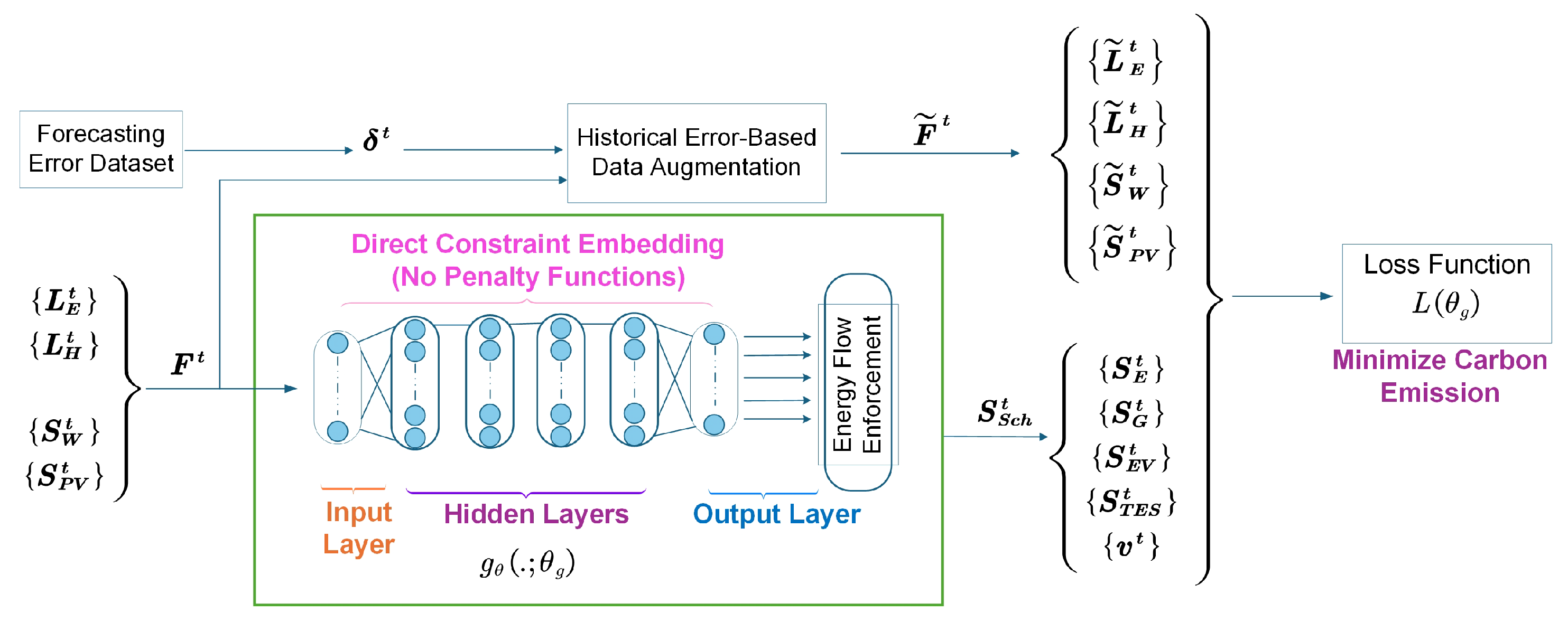
The proposed scheduling model is implemented as a fully connected DNN that maps forecast information into device-level operational decisions. The overall architecture, illustrated in Figure 3, is designed to balance representational power, training stability, and seamless integration with the constraint-embedding module.

The input layer processes forecast data across the 24-h horizon. For each time slot, five categories of features are included: electrical demand, thermal demand, wind generation forecast, photovoltaic generation forecast, and auxiliary temporal indicators such as time-of-day. Concatenated across all time steps, the resulting input dimension is 120, representing five feature types over a 24-h period.

The hidden representation is constructed using four fully connected layers with 360 neurons each. Each hidden layer incorporates a parametric rectified linear unit (PReLU) activation function [37], batch normalization [38], and a dropout layer with a rate of 0.3 for regularization [39]. This configuration provides sufficient capacity to model complex interactions between forecasts and optimal dispatch decisions while mitigating overfitting on augmented training scenarios.

The output layer produces 120 values corresponding to 24-h schedules for five device categories: transformer, CHP, boiler, EV, and TES. PV curtailment is not treated as an additional neural output. Instead, it is computed as a bounded residual variable during the DS balance evaluation, as defined in Equation (54). This preserves the 120-dimensional neural output while ensuring that severe PV overproduction is handled through physically admissible curtailment or inverter clipping. Instead of using these outputs directly, they are immediately processed by the feasibility-by-design decoder described in Section 2.2.   For non-memory fast devices (e.g., transformer and CHP), sigmoid-based scaling enforces instantaneous capacity limits. For memory devices such as EVs and TES, mean-offset corrections, clipping, and SOC trajectory scaling ensure net-zero energy alignment and SOC feasibility. For ramp-limited devices such as boilers, a ramp projection layer enforces inter-temporal ramp constraints. Embedding these transformations within the forward pass guarantees that every output schedule is physically feasible.

Through this architecture, the DNN produces complete day-ahead schedules without requiring penalty terms or post-hoc feasibility adjustments. Constraint embedding ensures that all outputs used in carbon-emission evaluation are intrinsically valid, and the differentiability of the constraint layers enables end-to-end learning of feasible and carbon-efficient dispatch strategies. In this way, the proposed model functions as a digital control component for sustainable smart-grid operation, linking renewable forecasts, energy storage flexibility, and carbon-aware scheduling decisions within a unified learning framework.

3.3. Data Augmentation for Uncertainty Handling

Forecast errors in load and renewable generation are unavoidable in practice, and schedules optimized solely for predicted trajectories may become infeasible or carbon-intensive during real operation. To account for this, the proposed framework incorporates a statistical data augmentation strategy that embeds uncertainty directly into the training process.

A database of historical relative forecast-error vectors is first constructed, containing multiplicative errors for electrical demand, thermal demand, wind generation, and photovoltaic (PV) generation. For a forecasted variable $x^t$, the historical relative error is defined as

$$\begin{array}{c}\hfill {\delta }_x^t={\displaystyle \frac{{\tilde{x}}^t-x^t}{x^t}},\end{array}$$

(56)

where $x^t$ denotes the day-ahead forecast and ${\tilde{x}}^t$ denotes the corresponding realized value. During training, an error vector is sampled from the historical error database and used to generate an augmented realization in a multiplicative form:

$$\begin{array}{c}\hfill {\tilde{x}}^t=\max \left(0, (1+{\delta }_x^t)x^t\right), x\in \{L_{\mathrm{elec}},L_{\mathrm{heat}},S_W\}.\end{array}$$

(57)

For PV generation, the relative forecast error is only evaluated during solar-available periods and is set to zero at night:

$$\begin{array}{c}\hfill {\delta }_{\mathrm{PV}}^t=\left\{\begin{array}{cc}{\displaystyle \frac{{\tilde{S}}_{\mathrm{PV}}^t-S_{\mathrm{PV}}^t}{S_{\mathrm{PV}}^t}}, \hfill & A_{\mathrm{PV}}^t=1, S_{\mathrm{PV}}^t>0,\hfill \\ 0, \hfill & A_{\mathrm{PV}}^t=0 \mathrm{or} S_{\mathrm{PV}}^t=0.\hfill \end{array}\right.\end{array}$$

(58)

Let $A_{\mathrm{PV}}^t\in \{0,1\}$ denote the solar-availability mask, where $A_{\mathrm{PV}}^t=1$ during daylight periods and $A_{\mathrm{PV}}^t=0$ during night-time periods. The augmented PV realization is therefore defined as

$$\begin{array}{c}\hfill {\tilde{S}}_{\mathrm{PV}}^t=A_{\mathrm{PV}}^t·\min \left[S_{\mathrm{PV},\max }^t,\max \left(0, (1+{\delta }_{\mathrm{PV}}^t)S_{\mathrm{PV}}^t\right)\right],\end{array}$$

(59)

where $S_{\mathrm{PV},\max }^t$ denotes the time-dependent upper envelope of physically available PV generation. This formulation prevents physically impossible PV realizations: when $A_{\mathrm{PV}}^t=0$ or $S_{\mathrm{PV}}^t=0$ at night, ${\tilde{S}}_{\mathrm{PV}}^t=0$ regardless of the sampled error term. During daylight periods, the non-negativity and upper-envelope clipping operations prevent negative PV output and PV generation exceeding the admissible solar envelope.

The complete augmented trajectory is denoted as

$$\begin{array}{c}\hfill {\tilde{F}}^t=\{{\tilde{L}}_{\mathrm{elec}}^t,{\tilde{L}}_{\mathrm{heat}}^t,{\tilde{S}}_W^t,{\tilde{S}}_{\mathrm{PV}}^t\}.\end{array}$$

(60)

The neural network receives the unperturbed forecast $F^t$ as input, while the augmented trajectory ${\tilde{F}}^t$ is used to compute the resulting carbon emissions. This exposes the model to historical forecast-error patterns while preserving the physical diurnal boundary of PV generation.

The learning objective is defined as the expectation of total carbon emissions with respect to the empirical distribution of forecast errors:

$$\begin{array}{c}\hfill \mathcal{L}\left(\theta \right)={\mathbb{E}}_{{\delta }^t}\left[E_{\mathrm{total}}\left({\tilde{F}}^t, g_{\theta }\left(F^t\right)\right)\right],\end{array}$$

(61)

where $g_{\theta }$ denotes the scheduling policy parameterized by the network weights $\theta$, and $E_{\mathrm{total}}$ is the carbon-emission model defined in (23). Optimizing this expected objective encourages the model to learn dispatch strategies that are robust in expectation, rather than overfitted to a single deterministic forecast [40].

This augmentation strategy provides two benefits. First, generalization is improved by exposing the neural scheduler to a wide range of historical error patterns, thereby reducing sensitivity to specific forecast scenarios. Second, the training process becomes aligned with the inherently stochastic nature of real-world operations, enabling the framework to generate carbon-efficient schedules that remain effective under both demand and renewable variability.

3.4. Day-Ahead Scheduling and Real-Time Adaptation

The final stage of the framework links the neural-network-based day-ahead scheduler with real-time operational data through the digital shadow (DS). This connection ensures that feasible schedules generated in advance remain valid under uncertainty, and that deviations from planned behavior can be monitored, corrected, and incorporated into subsequent training cycles.

In the day-ahead stage, the neural network receives the forecast input $F^t=\{L_{\mathrm{elec}}^t,L_{\mathrm{heat}}^t,S_W^t,S_{\mathrm{PV}}^t\}$ and produces device-level trajectories across the scheduling horizon. Because these outputs pass through the feasibility-by-design decoder described in Section 2.2, the resulting schedule satisfies all capacity, SOC, and ramping constraints by construction. The DS then archives this feasible plan and uses it as the reference trajectory for subsequent operation.

During real-time operation, actual system states ${\tilde{F}}^t$ differ from forecasts due to prediction errors. The DS continuously measures these deviations and computes the resulting imbalances that contribute to the extra-emission term. Fast-response non-memory devices, such as transformers and CHP units, are adjusted within their instantaneous capacities to compensate for imbalances. Memory devices such as EVs and TES continue to follow their pre-scheduled SOC trajectories to ensure long-term feasibility, while ramp-limited units such as boilers remain constrained by their ramp-rate limits as enforced by the ramp projection layer.

This division of operational responsibility balances robustness and stability: day-ahead schedules enforce feasible long-term trajectories for storage and ramp-limited devices, while real-time corrections are absorbed primarily by fast-response units. The DS closes the loop by recording deviations and feeding them back into the forecasting and training modules, thereby improving predictive accuracy and scheduling robustness over time.

Through this integration, the proposed method produces schedules that are feasible at first pass and robust to forecast uncertainty within the simulated DS environment, reducing the need for post-hoc correction in the scheduling layer.

4. Case Study and Results

4.1. Experimental Setup

The proposed scheduling framework is evaluated using a U.K. energy-system dataset covering the period from June 2023 to June 2024. The dataset includes paired forecasted and actual trajectories of electrical demand, PV generation, wind generation, thermal demand, and grid carbon intensity. Electrical demand, PV generation, and wind generation were collected from public U.K. settlement-period energy-system records, while the grid carbon-intensity data were obtained from the U.K. Carbon Intensity API developed by the National Energy System Operator (NESO, formerly National Grid ESO). Both forecasted and actual carbon-intensity values were used. Since measured heat-demand data were not available in the same format, the thermal-demand trajectory was generated from a normalized heat-load profile and scaled to match the IES case-study setting.

The raw data were originally available at 30-min settlement-period resolution, with 48 points per day. During dataset construction, the profiles were aligned and down-sampled to hourly resolution, resulting in a 24-h day-ahead scheduling horizon. The final model input contains 24-h forecasts of electrical demand, thermal demand, wind generation, PV generation, and time-related indicators, resulting in a 120-dimensional input vector. The model output contains 24-h schedules for five controllable device categories, including the transformer, CHP unit, boiler, EV storage, and TES.

Before training, abnormal or missing values were treated using variable-specific preprocessing. Isolated abnormal load and renewable-generation values were filled using adjacent settlement-period information. For PV generation, missing-data treatment was applied only within daylight periods to avoid introducing artificial night-time PV values. Carbon-intensity profiles outside the reasonable range were replaced using adjacent valid daily profiles. Forecast-error samples were then constructed from the relative differences between actual and forecasted trajectories and stored in an error database for uncertainty augmentation. After preprocessing and augmentation, the dataset contained 51,717 training samples and 357 evaluation samples. The training data were randomly divided into training, validation, and internal testing subsets with a ratio of 70%/20%/10%, while the final evaluation set was kept separate for reporting the results.

Table 1. Summary of the dataset and preprocessing procedure.

Item	Description
Region	United Kingdom
Study period	June 2023–June 2024
Raw resolution	30-min settlement-period data, 48 points/day
Scheduling resolution	Hourly, 24 time steps/day
Input variables	Electrical demand, thermal demand, wind generation, PV generation, and time indicators
Carbon-intensity data	Forecasted and actual values from the U.K. Carbon Intensity API developed by NESO, formerly National Grid ESO
Thermal demand	Generated from a normalized heat-load profile and scaled for the IES case study
Preprocessing	Data alignment, abnormal-value treatment, daylight-aware PV processing, and hourly down-sampling
Forecast-error database	Relative errors between actual and forecasted trajectories
Training samples	51,717 augmented daily samples
Evaluation samples	357 daily samples
Data split	70%/20%/10% training/validation/internal testing split

summarizes the dataset and preprocessing procedure.

In addition to the dataset preparation, the training configuration is reported to improve reproducibility. The proposed DNN was implemented in Python 3.12, using PyTorch 2.5.1 and trained with the AdamW optimizer. The learning rate was set to $1\times {10}^{-5}$, and the model was trained for 5000 epochs. Three batch-size settings, namely 1100, 1200, and 1300, were tested during training. The training, validation, and internal testing subsets followed a 70%/20%/10% random split. Training and validation losses were monitored every 100 epochs to assess convergence. The neural-network experiments were executed using CUDA acceleration when available, while the perfect-foresight optimization benchmark was solved in MATLAB R2025a using fmincon.

The detailed training settings are summarized in

Table 2. Summary of training settings.

Item	Setting
Implementation	Python/PyTorch
Optimizer	AdamW
Learning rate	$1\times {10}^{-5}$
Batch size	1200
Training epochs	5000
Data split	70%/20%/10% training/validation/internal testing
Convergence check	Training and validation losses monitored every 100 epochs
Benchmark solver	MATLAB fmincon

.

A forecast-driven day-ahead scheduler is adopted as the benchmark baseline. This baseline optimizes dispatch based solely on point forecasts, without explicit uncertainty modeling or carbon-aware penalties for real-time imbalances. As a result, deviations between forecasted and realized conditions are not represented in its objective, making it representative of common practice in deterministic IES scheduling.

In this case study, the EV subsystem is modeled as a contracted flexibility resource rather than as ordinary private EV mobility. Ordinary EV charging demand associated with daily travel behavior is included in the electrical load profile. The controllable EV resource represents vehicles or battery capacity contractually connected to the IES operator during the scheduling horizon. The base-case contract assumes that the EV resource is available for the full 24-h day-ahead scheduling period, so $A_{\mathrm{EV}}^{\mathrm{con},t}=1$ for all t. To ensure that the contract does not deplete the EV resource after the scheduling period, the terminal SOC condition $SO{C}_{\mathrm{EV}}^T=SO{C}_{\mathrm{EV}}^0$ is imposed. Therefore, the EV subsystem provides intra-day flexibility for carbon-aware scheduling while maintaining daily energy neutrality.

To quantify the theoretical limit of achievable performance, a perfect-foresight optimal solution is computed. In this setting, future realizations of demand, renewable generation, and carbon intensity are assumed to be known in advance. The resulting deterministic carbon-minimization problem is formulated as a constrained nonlinear program and solved using the fmincon solver in MATLAB. The perfect-foresight solution provides a lower bound on carbon emissions and serves as a reference for evaluating the proposed framework and the baseline.

4.2. Feasibility Verification

To quantitatively support the feasibility claim, all generated schedules are verified against the physical constraints defined in Section 2. For each testing day, the constraint residuals are calculated after the feasibility-by-design decoder. A schedule is considered feasible only if all capacity, power-limit, SOC-bound, and terminal consistency constraints are satisfied within a numerical tolerance of $ϵ={10}^{-3}$. The testing set contains 357 day-ahead schedules, corresponding to 8568 hourly operating points.

Table 3. Quantitative feasibility verification of generated schedules.

Constraint Category	Metric	Maximum Violation	Violation Rate
Transformer capacity	$0\le S_E^t\le S_{\mathrm{TF}}^{\max }$	0	0%
CHP capacity	$0\le P_{\mathrm{CHP}}^t\le S_{\mathrm{CHP}}^{\max }$	0	0%
Boiler capacity	$0\le P_B^t\le S_B^{\max }$	0	0%
EV power limit	$-P_{\mathrm{EV}}^{\max ,\mathrm{Ch}}\le P_{\mathrm{EV}}^t\le P_{\mathrm{EV}}^{\max ,\mathrm{Dis}}$	$1.50\times {10}^{-5}$	0%
EV SOC bounds	$SO{C}_{\mathrm{EV}}^{\min }\le SO{C}_{\mathrm{EV}}^t\le SO{C}_{\mathrm{EV}}^{\max }$	$4.80\times {10}^{-5}$	0%
EV terminal consistency	$|SO{C}_{\mathrm{EV}}^T-SO{C}_{\mathrm{EV}}^0|$	$1.87\times {10}^{-4}$	0%
TES power limit	$-P_{\mathrm{TES}}^{\max ,\mathrm{Ch}}\le P_{\mathrm{TES}}^t\le P_{\mathrm{TES}}^{\max ,\mathrm{Dis}}$	$3.10\times {10}^{-5}$	0%
TES SOC bounds	$SO{C}_{\mathrm{TES}}^{\min }\le SO{C}_{\mathrm{TES}}^t\le SO{C}_{\mathrm{TES}}^{\max }$	$1.14\times {10}^{-4}$	0%
TES terminal consistency	$|SO{C}_{\mathrm{TES}}^T-SO{C}_{\mathrm{TES}}^0|$	$5.76\times {10}^{-4}$	0%
Overall schedule feasibility	–	–	100%

reports the feasibility verification results over the complete testing set. The transformer, CHP, and boiler capacity constraints have zero maximum violation. The maximum EV and TES power-limit residuals are $1.50\times {10}^{-5}$ and $3.10\times {10}^{-5}$, respectively, while the maximum SOC-bound residuals are $4.80\times {10}^{-5}$ for EVs and $1.14\times {10}^{-4}$ for TES. The maximum terminal consistency residuals are $1.87\times {10}^{-4}$ and $5.76\times {10}^{-4}$ for EVs and TES, respectively. All these residuals are below the numerical tolerance, and no constraint violation is detected. Therefore, the overall schedule feasibility rate reaches 100%.

These results confirm that the proposed decoder enforces physical feasibility by construction and that the generated schedules do not require post-hoc repair before deployment in the DS environment.

4.3. Effectiveness of the Constraint-Embedded Decoder

To verify the effectiveness and necessity of the proposed feasibility-by-design decoder, an ablation study is conducted by comparing the full proposed model with a variant in which the constraint-embedded decoder is removed. In the ablated variant, the neural network output is processed only by simple clipping and conventional post-processing, without SOC-trajectory enforcement or ramp-constraint projection. Therefore, this variant represents a typical penalty/post-processing-based learning scheduler and is used to examine whether explicit constraint embedding is necessary for physically executable scheduling.

Table 4. Ablation study on the constraint-embedded decoder.

Model Variant	Feasibility	Infeasible Samples	Total Carbon Objective
Full proposed model	$100.0\%\pm 0.0\%$	$0/357$	$(2.425\pm 0.047)\times {10}^9$
Without constraint-embedded decoder	$0.0\%\pm 0.0\%$	$357/357$	$(1.812\pm 0.228)\times {10}^9$

summarizes the results over five random seeds on the 357-sample testing set. The full proposed model achieves 100% feasibility for all testing samples, with no infeasible schedules observed. In contrast, removing the constraint-embedded decoder results in 0% feasibility, with all 357 testing samples violating at least one physical constraint. The largest violations occur in the SOC-related constraints of the EV and TES subsystems, confirming that simple clipping cannot correctly handle inter-temporal storage dynamics.

It should be noted that the ablated model without the decoder produces a lower numerical carbon objective. However, this value is not physically meaningful because it is obtained from infeasible schedules that cannot be deployed in practice. In other words, the apparent emission reduction is achieved by violating operational constraints rather than by producing a realizable low-carbon dispatch. By contrast, the full proposed model maintains complete feasibility while optimizing the carbon objective, demonstrating that the feasibility-by-design decoder is an essential architectural component rather than a cosmetic post-processing step.

4.4. Robustness Under Extreme Forecast Errors

To further evaluate the robustness of the proposed framework under degraded forecast quality, additional simulations are conducted under different forecast-error levels. In this experiment, the full proposed model is tested under multiplicative Gaussian forecast noise levels of 0%, 5%, 10%, 20%, and 30%. The noise is applied only to the physical forecast variables, including electrical demand, thermal demand, wind generation, and PV generation, while the carbon-intensity input is kept unchanged. The actual realization used for emission evaluation is also unchanged. Therefore, this experiment isolates the impact of forecast degradation on scheduling performance rather than changing the physical system or carbon-intensity profile.

For each forecast-error level, five independent runs are conducted using different random seeds.

Table 5. Robustness analysis under different forecast-error levels.

Forecast Error	Total Emission Index ($\times {\mathbf{10}}^{\mathbf{9}}$)	Scheduled Emission Index ($\times {\mathbf{10}}^{\mathbf{9}}$)	Imbalance Emission Index ($\times {\mathbf{10}}^{\mathbf{9}}$)	Increase (%)	Feasibility (%)
0%	$2.425\pm 0.047$	$1.540\pm 0.007$	$0.884\pm 0.042$	–	$100.0\pm 0.0$
5%	$2.566\pm 0.056$	$1.540\pm 0.007$	$1.027\pm 0.052$	5.8	$100.0\pm 0.0$
10%	$2.879\pm 0.056$	$1.537\pm 0.005$	$1.342\pm 0.051$	18.7	$100.0\pm 0.0$
20%	$3.592\pm 0.073$	$1.522\pm 0.006$	$2.070\pm 0.071$	48.1	$100.0\pm 0.0$
30%	$4.304\pm 0.138$	$1.510\pm 0.015$	$2.794\pm 0.134$	77.5	$100.0\pm 0.0$

reports the mean and standard deviation of total emission index, scheduled emission index, imbalance emission index, and feasibility rate. As the forecast-error level increases from 0% to 30%, the total emission index increases from $2.425\pm 0.047$ to $4.304\pm 0.138$, corresponding to a 77.5% increase relative to the no-additional-noise case. This increase is mainly caused by the growth of imbalance-related emissions, which increase from $0.884\pm 0.042$ to $2.794\pm 0.134$. In contrast, the scheduled emission component remains comparatively stable, indicating that severe forecast errors mainly affect the real-time correction burden rather than the nominal day-ahead schedule.

Importantly, the proposed framework maintains a 100% feasibility rate under all tested forecast-error levels. The maximum SOC and capacity violations remain at the numerical tolerance level, confirming that the feasibility-by-design decoder continues to enforce physical constraints even when the forecast input is severely degraded. These results demonstrate that forecast errors primarily degrade carbon performance through increased imbalance emissions, while operational feasibility remains protected by the constraint-embedded neural decoder.

4.5. Economic Indicators and Carbon–Cost Extension

Although the primary objective of this work is carbon-aware scheduling, economic performance is also an important factor for practical engineering deployment. Therefore, the proposed carbon-first framework can be naturally extended to include operating-cost indicators. The total operating cost of a generated schedule can be expressed as

$$\begin{array}{c}\hfill C_{\mathrm{op}}={\displaystyle \sum _{t=1}^T}\left(c_{\mathrm{grid}}^t{S}_E^t+c_{\mathrm{gas}}{S}_G^t+c_{\mathrm{gas}}{S}_B^t+c_{\mathrm{EV}}^{\mathrm{deg}}\left|P_{\mathrm{EV}}^t\right|+c_{\mathrm{TES}}^{\mathrm{op}}\left|P_{\mathrm{TES}}^t\right|\right)\Delta t,\end{array}$$

(62)

where $c_{\mathrm{grid}}^t$ is the time-varying electricity purchase price, $c_{\mathrm{gas}}$ is the natural-gas price, $c_{\mathrm{EV}}^{\mathrm{deg}}$ denotes the EV battery degradation cost coefficient, and $c_{\mathrm{TES}}^{\mathrm{op}}$ denotes the TES operation-related cost coefficient. This metric provides a direct way to evaluate whether a low-carbon schedule introduces an excessive economic burden.

A carbon–cost multi-objective extension can then be formulated as

$$\begin{array}{c}\hfill J_{\mathrm{CE}}={\omega }_C{\displaystyle \frac{E_{{\mathrm{CO}}_2}}{E_{{\mathrm{CO}}_2}^{\mathrm{base}}}}+{\omega }_K{\displaystyle \frac{C_{\mathrm{op}}}{C_{\mathrm{op}}^{\mathrm{base}}}}, {\omega }_C+{\omega }_K=1,\end{array}$$

(63)

where $E_{{\mathrm{CO}}_2}^{\mathrm{base}}$ and $C_{\mathrm{op}}^{\mathrm{base}}$ denote the carbon emission and operating cost of a reference baseline, respectively. The weights ${\omega }_C$ and ${\omega }_K$ allow system operators to adjust the relative importance of carbon reduction and economic performance. When ${\omega }_C$ is larger, the scheduler prioritizes emission reduction; when ${\omega }_K$ is larger, the scheduler gives more emphasis to operating-cost reduction.

The present study focuses on the carbon-first case because its central aim is to evaluate whether a feasibility-by-design neural scheduler can directly reduce scheduled and imbalance-driven emissions under forecast uncertainty. However, Equations (62) and (63) show that the same framework can be extended to practical carbon–cost decision support without changing the proposed constraint-embedded decoder. In this extension, the decoder continues to guarantee physical feasibility, while the objective function can be adjusted to reflect different operator preferences regarding carbon emissions, cost, reliability, and system risk.

4.6. Daily Performance Analysis

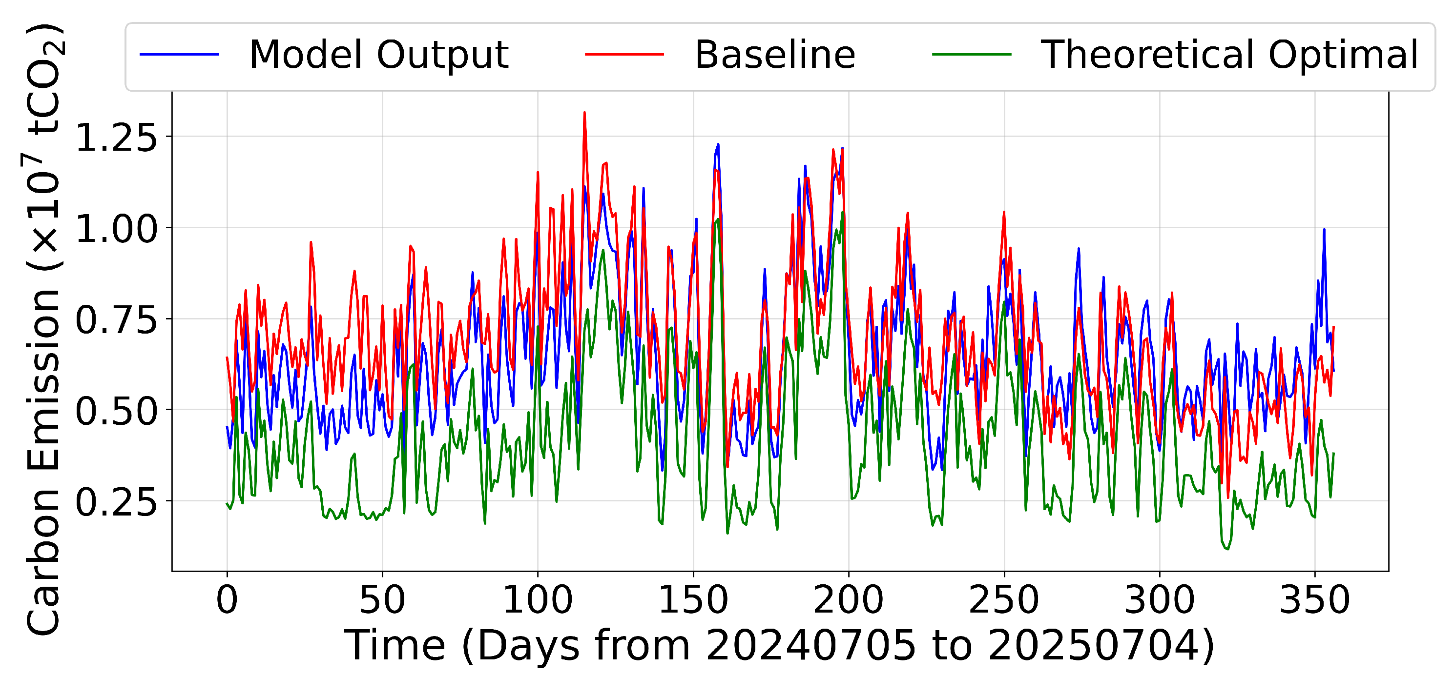
Figure 4 reports the daily carbon emissions produced by the proposed method, the forecast-driven baseline, and the theoretical optimum across the testing horizon. The proposed framework consistently outperforms the baseline, achieving an average emission reduction of approximately 4.0%. This indicates that the feasibility-by-design decoder and carbon-aware objective successfully shift operational decisions toward lower-emission trajectories while maintaining physical feasibility.

When compared with the perfect-foresight optimum, the proposed model exhibits a mean gap of $2.35\times {10}^6$ tCO₂, corresponding to an average relative distance of 71.0%. This discrepancy primarily reflects forecast uncertainty and device constraints that limit the extent to which flexibility can be exploited. Normalizing performance within the interval defined by the baseline–optimum range shows that the proposed model achieves a relative score of 0.975, demonstrating that it moves the schedule toward the theoretical low-carbon optimum while still operating under realistic forecast uncertainty and device constraints.

Seasonal patterns are apparent in the daily trajectories. During winter months, where both demand levels and renewable variability are higher, emissions increase for all methods. Nonetheless, the proposed model maintains a consistent margin over the baseline, suggesting that uncertainty-aware training improves robustness under highly variable conditions. Occasional peaks in the daily emission profile indicate opportunities for further enhancements, such as rolling-horizon re-optimization or improved short-term forecasting. Even so, the smoother trajectory produced by the proposed approach suggests that fewer aggressive corrective actions are required in real time.

4.7. Statistical Significance Analysis

To further support the reported emission-reduction performance, a day-level paired statistical analysis is conducted over the full testing year. For each testing day, the daily CO₂ emissions of the forecast-driven baseline and the proposed method are compared using the same demand, renewable-generation, and carbon-intensity conditions. This paired setting directly evaluates whether the daily reduction achieved by the proposed framework is statistically consistent rather than being driven by a small number of favorable days.

Let $E_d^{\mathrm{base}}$ and $E_d^{\mathrm{prop}}$ denote the daily CO₂ emissions of the forecast-driven baseline and the proposed method on testing day d, respectively. The daily relative emission reduction is calculated as

$$\begin{array}{c}\hfill r_d={\displaystyle \frac{E_d^{\mathrm{base}}-E_d^{\mathrm{prop}}}{E_d^{\mathrm{base}}}}\times 100\%.\end{array}$$

(64)

The mean reduction, standard deviation, and 95% confidence interval are then computed across all testing days. In addition, a paired t-test is applied to the daily emission pairs $\{E_d^{\mathrm{base}},E_d^{\mathrm{prop}}\}$, and a Wilcoxon signed-rank test is also reported as a non-parametric robustness check.

Table 6. Statistical significance analysis of daily CO₂ emission reduction.

Metric	Value	Description
Testing days	365	Number of paired daily samples
Baseline annual emissions	8.603 Mt CO2	Forecast-driven baseline
Proposed annual emissions	8.250 Mt CO2	Proposed framework
Annual emission reduction	4.10%	Annual total reduction
Mean daily reduction	4.10%	Average daily relative reduction
Standard deviation	1.63%	Daily relative reduction variability
95% confidence interval	3.94–4.27%	Confidence interval of daily reduction
Paired t-test	$p=1.00\times {10}^{-155}$	Parametric significance test
Wilcoxon signed-rank test	$p=1.00\times {10}^{-62}$	Non-parametric robustness check

summarizes the statistical results. Across 365 testing days, the proposed method reduces daily CO₂ emissions by 4.10% on average, with a standard deviation of 1.63%. The 95% confidence interval is 3.94%–4.27%, which does not include zero. The paired t-test gives $p=1.00\times {10}^{-155}$, and the Wilcoxon signed-rank test gives $p=1.00\times {10}^{-62}$. These results indicate that the emission reduction is statistically significant at the 5% level. At the annual scale, the total emissions are 8.603 Mt CO₂ for the forecast-driven baseline and 8.250 Mt CO₂ for the proposed method, corresponding to an annual reduction of 4.10%.

4.8. Monthly Aggregated Results

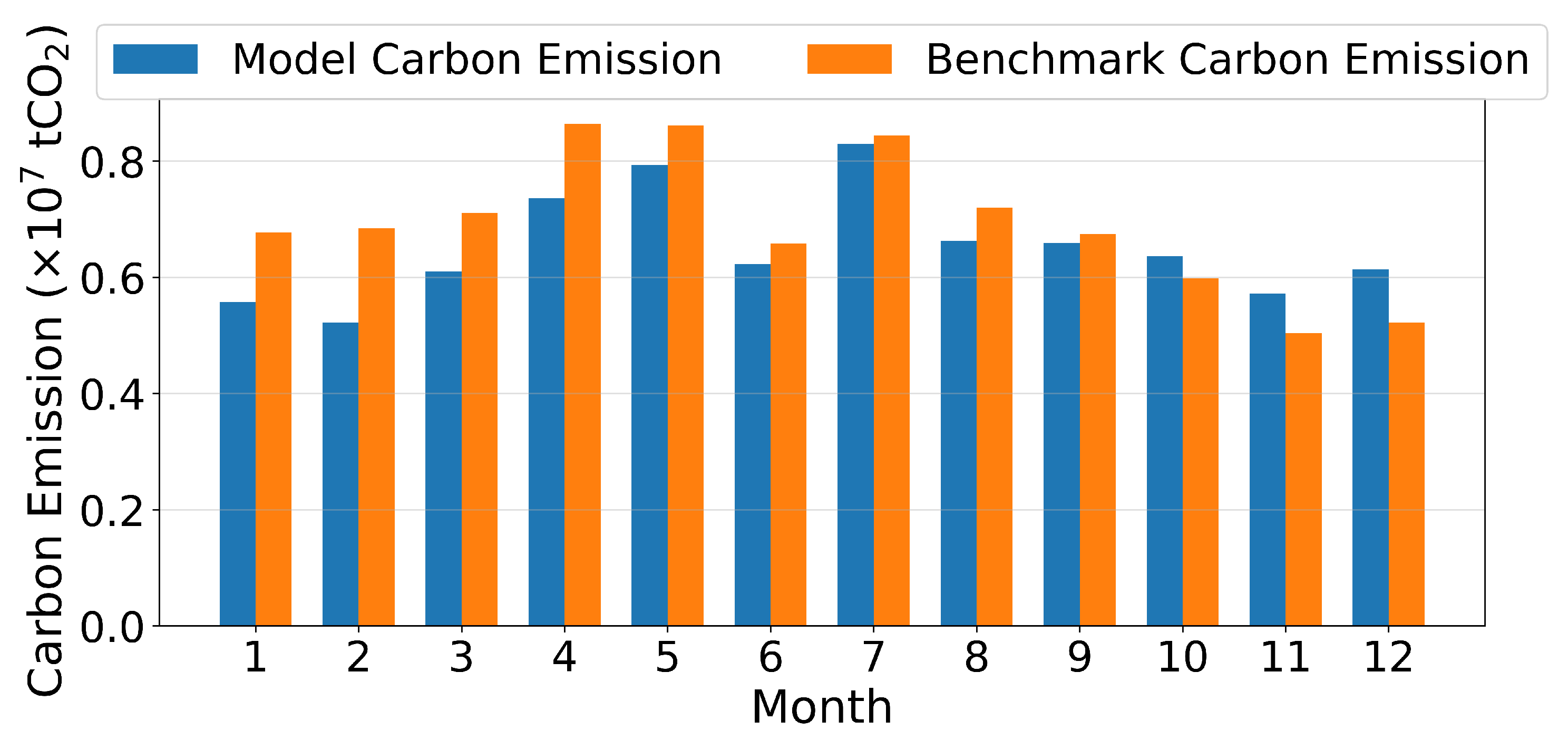
To evaluate long-term performance and seasonal trends, Figure 5 compares the monthly aggregated carbon emissions of the proposed framework against the forecast-driven baseline. Across all twelve months, the proposed method achieves consistent reductions, with improvements ranging from approximately 2% to over 6%. The average monthly reduction aligns with the daily analysis, yielding an overall decrease of around 4.0% relative to the baseline.

Seasonal differences are clearly observable. During high-demand winter months (January, February, and December), the framework achieves the largest reductions. In these periods, both the system load and marginal carbon intensity tend to be elevated, increasing the value of flexibility from EVs and TES. The proposed model allocates storage and dispatchable resources more effectively, reducing reliance on high-carbon imports and smoothing peak-emission episodes. In contrast, the reductions are somewhat smaller during spring and early summer (April–June), when renewable availability is higher and overall system demand is lower, thereby reducing the marginal benefit of flexibility.

Overall, the monthly results confirm that the proposed method delivers sustained emission reductions over longer temporal horizons. The consistent advantage observed across all months highlights the robustness of the feasibility-by-design decoder and the carbon-aware objective across diverse seasonal conditions.

4.9. Seasonal Dispatch Comparison

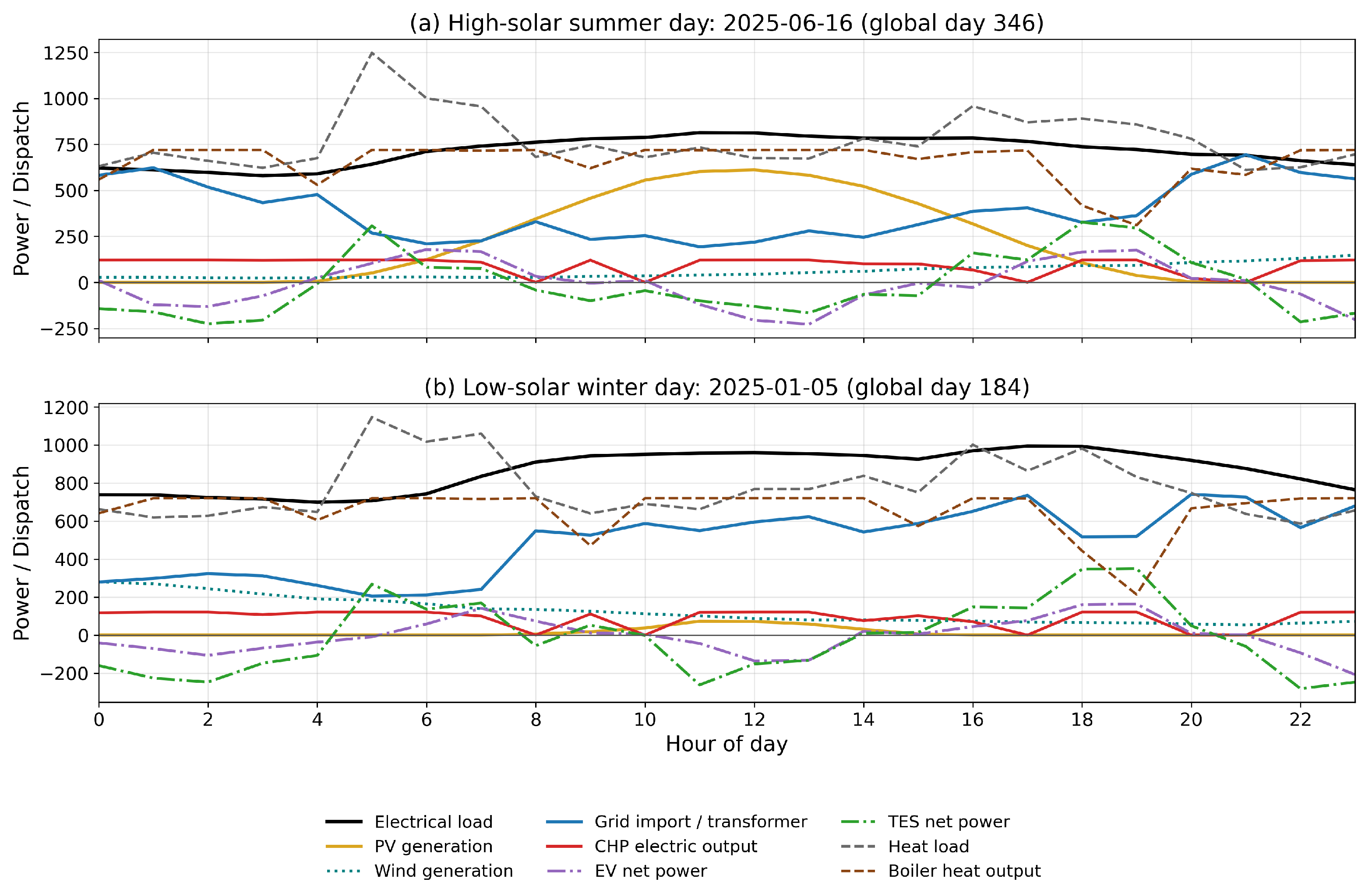
To provide direct visual evidence of the seasonal dispatch behaviour of the proposed framework, a representative 24-h comparison is conducted between a high-solar summer day and a low-solar winter day. The selected summer day is 16 June 2025, with a total daily PV generation of 5176.45 MWh and a total electrical load of 17,111.87 MWh. The selected winter day is 5 January 2025, with a total daily PV generation of 299.62 MWh and a total electrical load of 20,733.67 MWh.

Figure 6 compares the hourly dispatch schedules generated by the proposed framework under these two seasonal conditions. In the high-solar summer case, the scheduler makes greater use of renewable generation and coordinates grid import, CHP/boiler output, EV operation, and TES operation to accommodate the higher midday PV availability. In the low-solar winter case, the reduced PV contribution and higher electrical demand lead to greater reliance on dispatchable resources and grid imports.

This comparison shows that the proposed neural scheduler adapts its dispatch pattern according to seasonal renewable availability and demand variation. The summer case highlights the coordination of renewable generation and flexible storage during high-PV periods, whereas the winter case demonstrates the importance of carbon-aware allocation among grid imports, CHP, boiler output, EV flexibility, and TES operation under lower PV availability and higher demand.

4.10. Fine-Grained Temporal Analysis

To provide a more detailed understanding of temporal behavior, additional comparisons are conducted at daily and hourly resolutions. These analyses highlight how the proposed model reshapes operational decisions not only over months or days but also within individual hours.

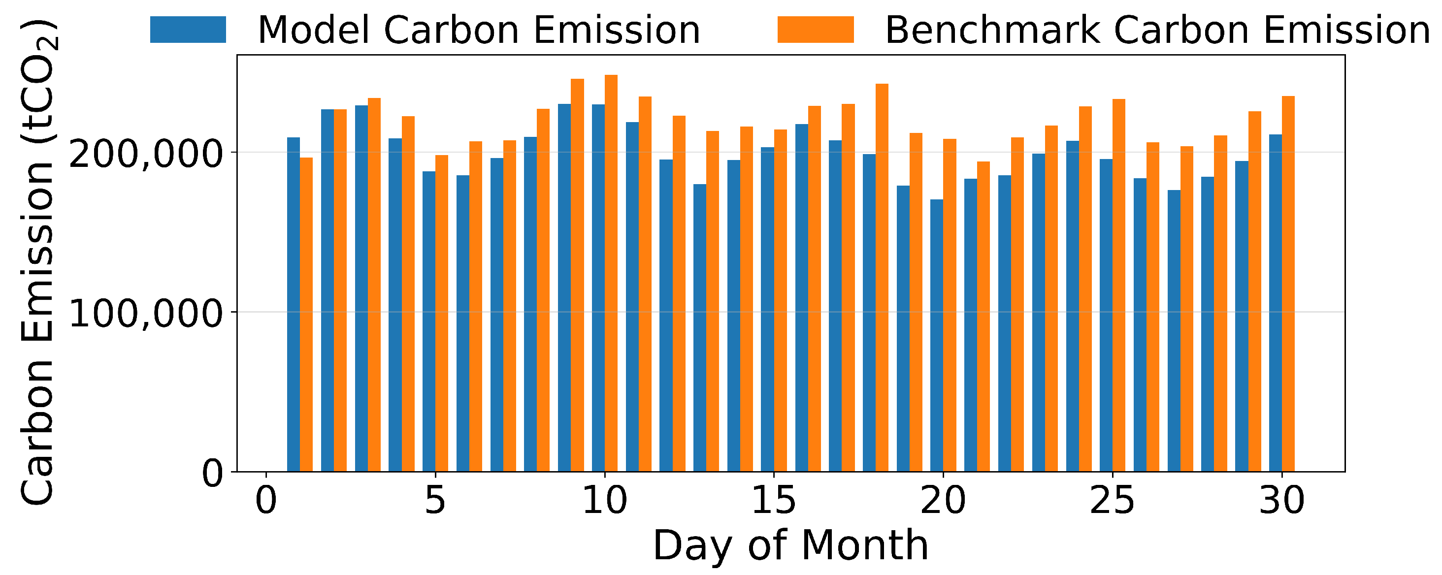
Figure 7 reports the daily carbon emissions within a representative month. The proposed framework exhibits lower emissions than the baseline on nearly all days, with reductions of several percent on typical days. This demonstrates that the advantages observed at annual and monthly scales also persist under shorter-term variability, indicating that the feasibility-by-design decoder responds robustly to fluctuations in demand and renewable availability.

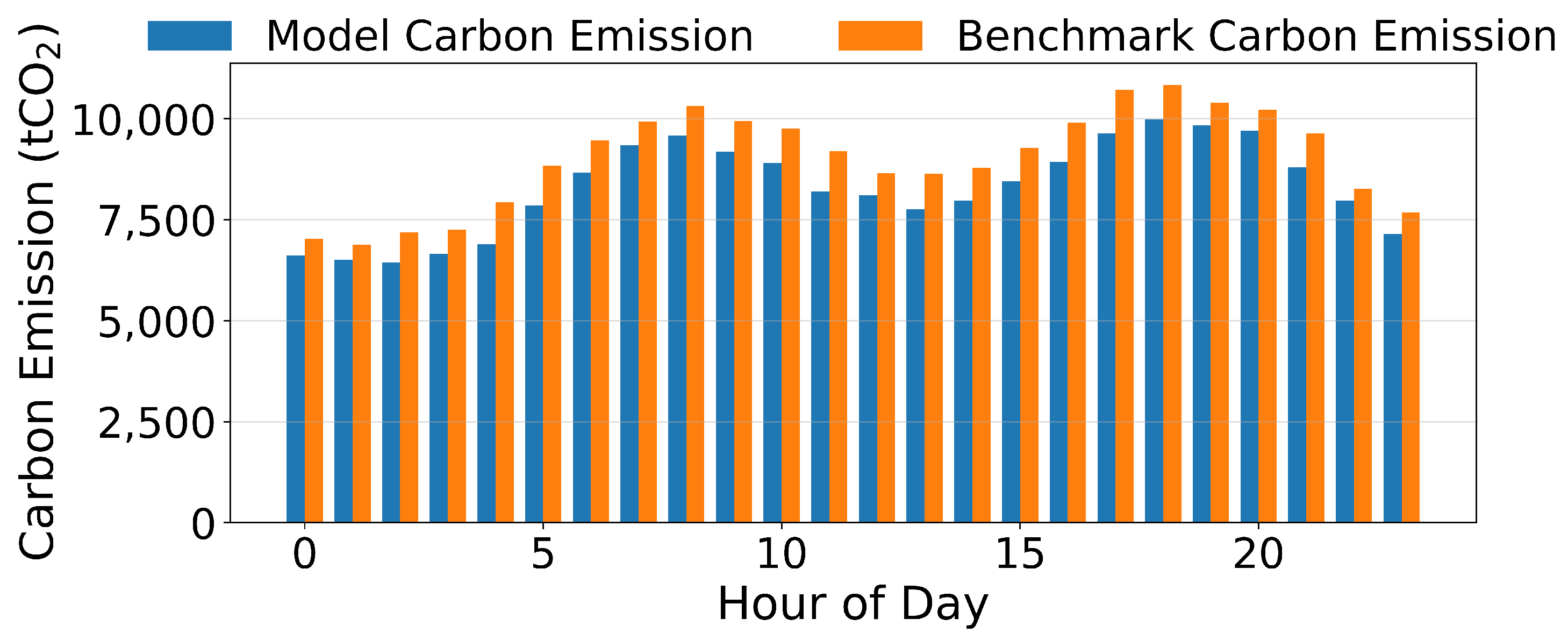
A further breakdown at the hourly level is shown in Figure 8 for a representative day. Both the baseline and the proposed model display the expected diurnal structure, with emissions peaking during evening load surges. However, the proposed model consistently schedules lower hourly emissions throughout the day, with the greatest reductions occurring during peak hours. This indicates that the carbon-aware objective does not merely shift energy temporally but actively reshapes dispatch patterns to avoid high-carbon periods when possible.

Taken together, the fine-grained analyses demonstrate that the proposed framework delivers improvements at every temporal scale—annual, monthly, daily, and hourly. The consistency of these reductions underscores the robustness and practical value of integrating constraint embedding with a carbon-aware objective in data-driven scheduling.

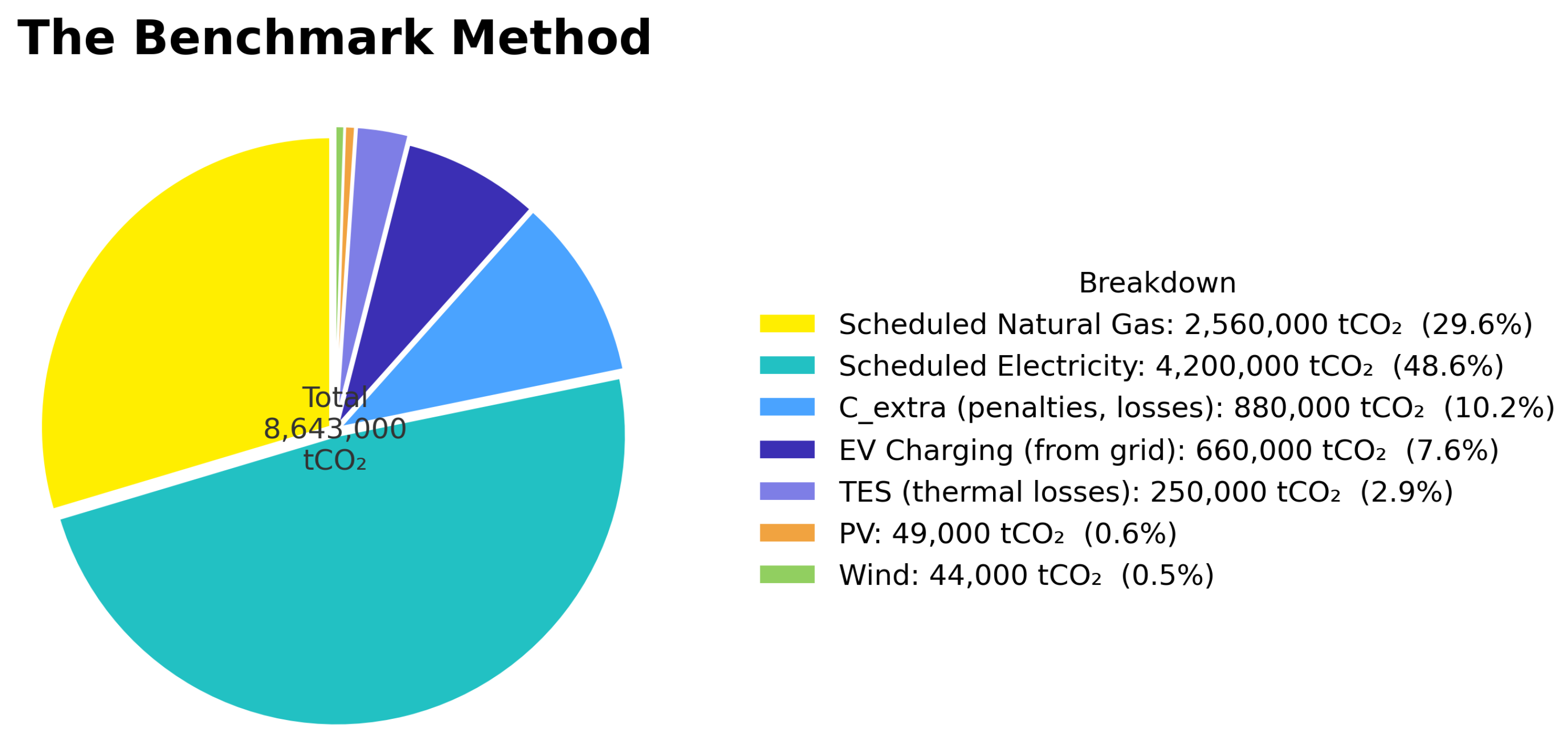
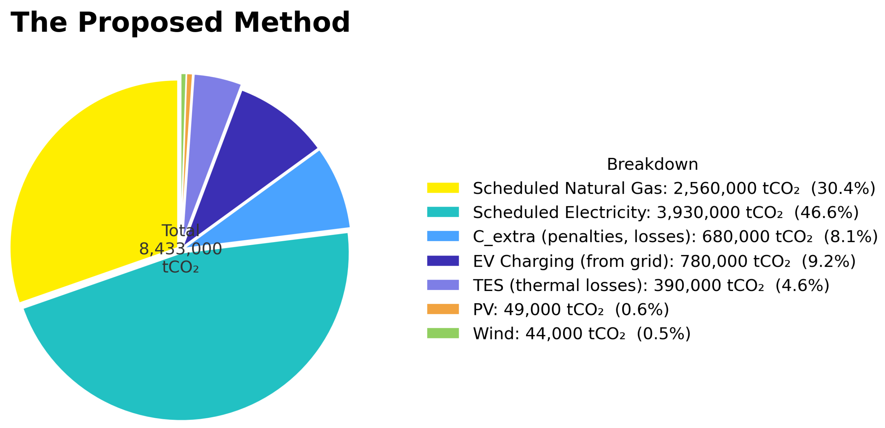
4.11. Emission Source Breakdown

To better understand how the proposed framework achieves carbon reductions, Figure 9 and Figure 10 present the composition of total emissions by source for both the benchmark and the proposed method. This decomposition highlights how the carbon-aware objective and embedded constraints reshape dispatch behavior and utilization of flexible resources.

In the benchmark case (Figure 9), scheduled electricity imports dominate the emission profile, contributing 4.20 million tCO₂ (48.6%), followed by scheduled natural gas use at 2.56 million tCO₂ (29.6%). Additional mismatch-driven penalties account for 0.88 million tCO₂ (10.2%), reflecting substantial real-time deviations from the day-ahead plan. EV charging from the grid and TES thermal losses contribute 7.6% and 2.9%, respectively. Overall, the emission distribution indicates heavy dependence on high-carbon electricity and significant penalties due to forecast-induced imbalances.

By contrast, the proposed framework generates a different emission profile (Figure 10). Emissions from scheduled electricity decrease to 3.93 million tCO₂ (46.6%), and mismatch-related emissions $E_{\mathrm{extra}}$ fall markedly to 0.68 million tCO₂ (8.1%), indicating that the day-ahead schedules generated by the feasibility-by-design decoder are more consistent with real-time system conditions. At the same time, the shares associated with EV charging (9.2%) and TES thermal losses (4.6%) increase, reflecting enhanced utilization of flexible storage devices to mitigate variability and reduce dependence on the grid during high-carbon periods. These changes in operational behavior reduce total emissions from 8.64 to 8.29 million tCO₂.

Overall, the breakdown reveals a shift in scheduling priorities. The benchmark relies predominantly on direct electricity imports and incurs significant penalties from real-time deviations, while the proposed method strategically leverages EVs and TES as flexibility buffers. This reallocation reduces both scheduled and mismatch-driven emissions, demonstrating the effectiveness of the carbon-aware objective and constraint-embedded neural architecture.

4.12. Discussion

The results demonstrate the effectiveness of embedding device-level constraints and carbon-aware objectives within a deep learning framework for sustainable power-system scheduling. Across daily, monthly, and fine-grained temporal analyses, the proposed method consistently outperforms the forecast-driven baseline, achieving an average reduction of approximately 4.0% in total carbon emissions. These improvements are achieved without post-hoc feasibility repair, confirming that the feasibility-by-design decoder successfully aligns neural outputs with physical operating requirements while optimizing against time-varying carbon intensity. From a smart-grid operation perspective, the framework improves the coordination of renewable generation, energy storage flexibility, and conventional dispatchable devices under forecast uncertainty.

Despite these gains, a substantial gap remains relative to the theoretical optimum. On average, the proposed schedules exhibit a difference of $2.35\times {10}^6$ tCO₂ from the ideal benchmark (approximately 71% above the optimal level). In normalized terms, the model occupies a relative position of 0.975 within the baseline–optimum interval. This indicates meaningful improvement over conventional scheduling but also highlights the challenges posed by forecast uncertainty and strict device constraints. Ramping limits and SOC bounds restrict the full exploitation of flexibility, particularly during high-demand and high-carbon-intensity periods.

Temporal analysis further suggests that the model performs most effectively under moderate operating conditions, while winter peaks remain more challenging. The larger improvements observed in high-carbon winter months indicate that the carbon-aware objective successfully prioritizes the use of flexibility when it is most valuable. However, residual emission peaks imply that additional adaptation mechanisms—such as rolling-horizon updates, probabilistic forecasts, or hybrid model-based and data-driven scheduling—could narrow the remaining gap to the theoretical optimum.

Overall, the discussion highlights that while the proposed methodology delivers consistent carbon reductions and guaranteed feasibility, its performance is ultimately bounded by prediction accuracy and physical limitations. Addressing these factors represents a promising direction for future development and deployment of carbon-conscious scheduling tools.

From a sustainability perspective, the proposed framework contributes to the low-carbon energy transition by improving the operational use of renewable generation and energy storage resources. The reduction in mismatch-related emissions suggests that digital-shadow-assisted scheduling can reduce reliance on high-carbon emergency balancing actions, which is particularly important for future smart grids with high renewable penetration. Therefore, the proposed method provides not only a technical scheduling tool but also a practical decision-support framework for sustainable power-system operation, renewable integration, and carbon-emission reduction.

4.13. Comparison with a Representative CNN–BiLSTM Scheduling Model

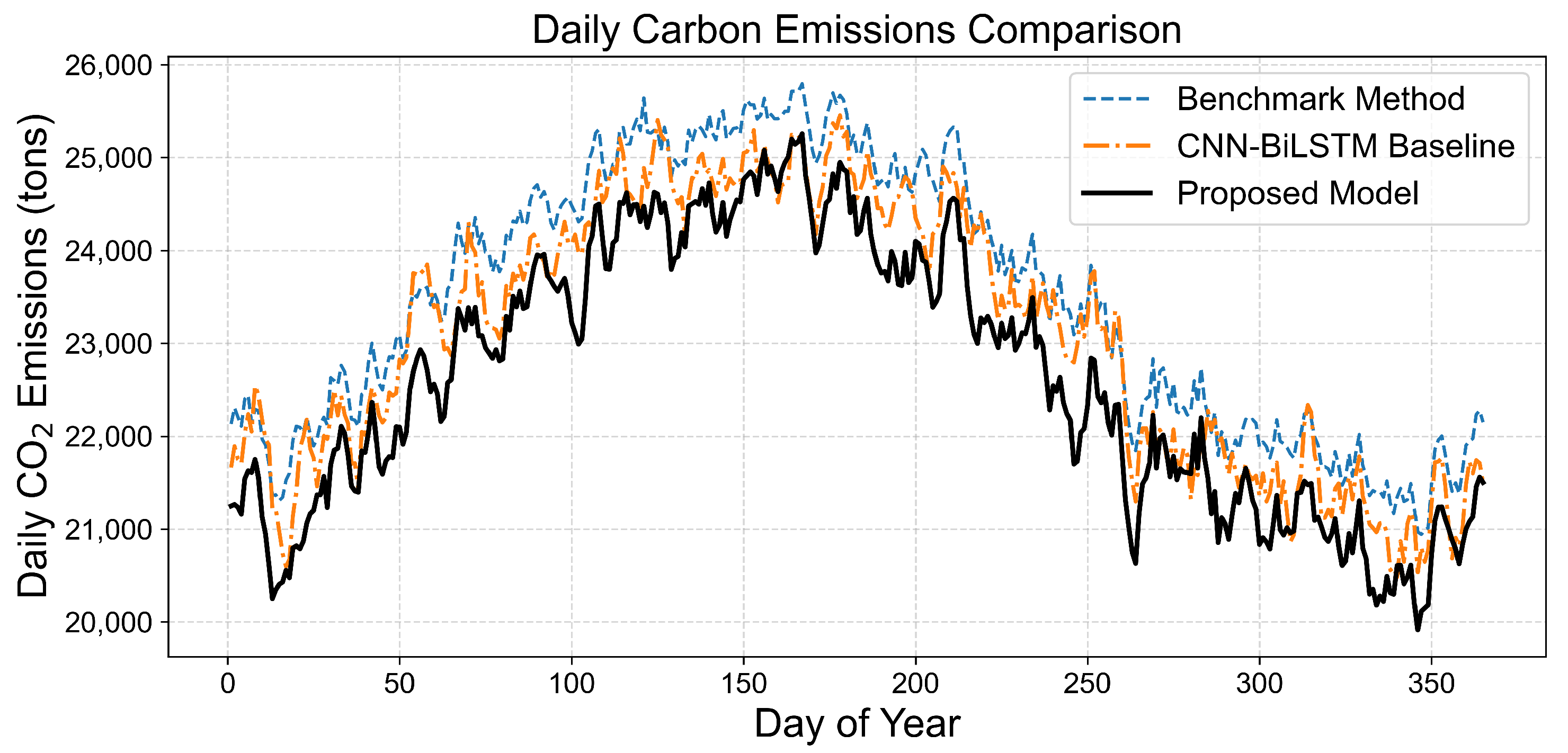
To benchmark the proposed framework against an established deep learning approach, a representative CNN–BiLSTM-based scheduling model [41] is reimplemented and evaluated under identical experimental conditions. The baseline combines convolutional layers for spatial feature extraction with bidirectional LSTMs for temporal modeling, and is trained using supervised learning to minimize the mean-squared error between predicted and optimization-derived schedules. Physical constraints are enforced through post-processing procedures such as power clipping and balance correction. For a fair comparison, the CNN–BiLSTM model is trained and tested using the same data split, input variables, forecast-error augmentation strategy, and carbon-emission evaluation environment as the proposed framework. The benchmark model follows the conventional learning-based scheduling pipeline reported in the literature: it first predicts device-level schedules and then applies external post-processing steps, including power clipping, balance correction, and SOC/ramp-feasibility adjustment, to reduce physical violations. It should be noted that the proposed feasibility-by-design decoder is not attached to the CNN–BiLSTM baseline. This choice is intentional because the decoder is the main methodological contribution of this paper; adding it to the CNN–BiLSTM model would create a hybrid “CNN–BiLSTM + proposed decoder” ablation rather than an independent literature baseline. Therefore, the comparison in this section should be interpreted as a framework-level comparison between a representative post-processing-based deep learning scheduler and the proposed constraint-embedded carbon-aware scheduler, rather than as a claim that the feed-forward neural architecture alone is superior to CNN–BiLSTM.

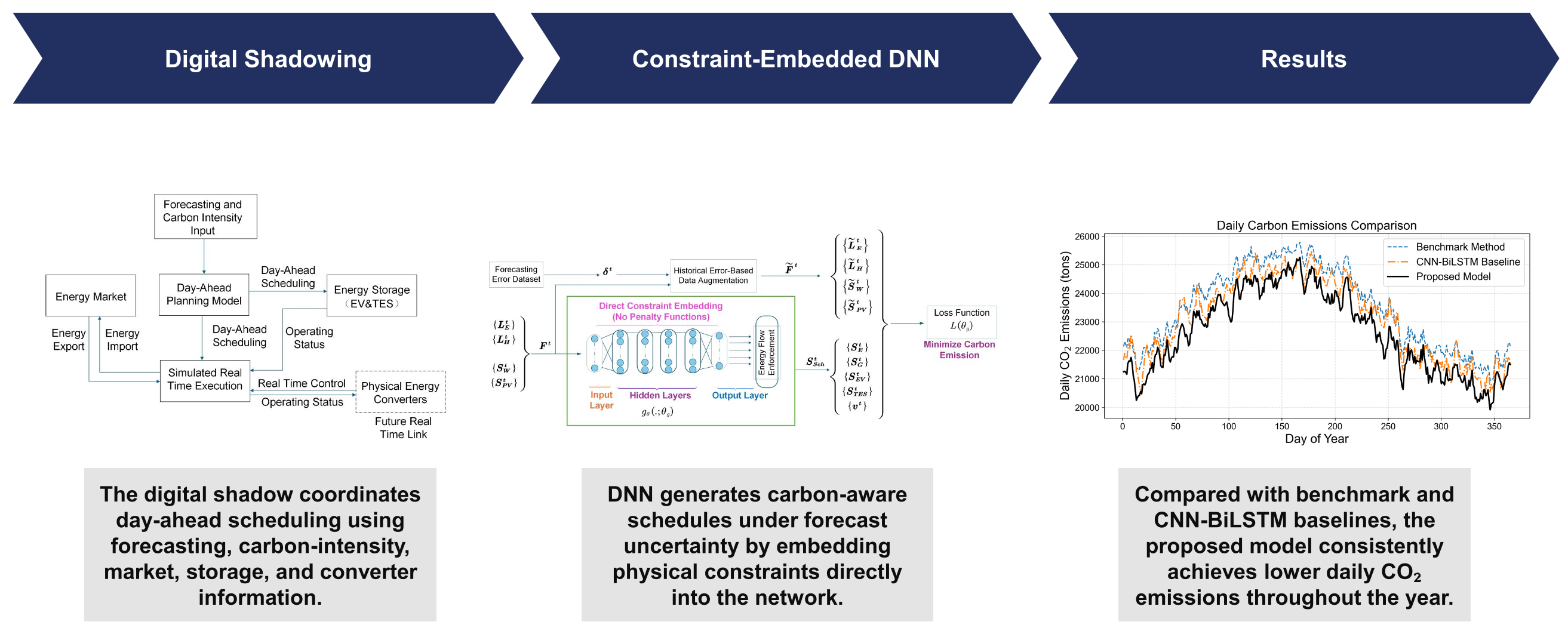
Figure 11 presents daily emission profiles for the CNN–BiLSTM baseline, the forecast-driven reference, and the proposed model. The CNN–BiLSTM achieves modest carbon reductions relative to the forecast-based strategy (average improvement ∼1.6%), indicating that temporal feature extraction is beneficial for data-driven scheduling. However, its performance remains lower than that of the proposed framework. This difference should be attributed not only to the neural architecture but also to the overall scheduling design, including the embedded feasibility mechanism and the carbon-first objective. The CNN–BiLSTM baseline relies on external repair after prediction and may still require correction when SOC or ramping constraints are violated, whereas the proposed framework incorporates these constraints into the forward pass and therefore produces feasible schedules without post-hoc repair.

Table 7. Annual carbon performance comparison.

Model	Feasibility	CO2 (Mt)	Gap to Opt. (Mt)
Forecast-based	85.3%	8.64	+2.57
CNN–BiLSTM	91.2%	8.50	+2.43
Proposed	100%	8.29	+2.21

summarizes annual performance. Although the CNN–BiLSTM baseline benefits from improved representation learning, its lack of embedded constraint handling and absence of a carbon-centric objective limit its efficacy in carbon-critical environments. The proposed model achieves lower emissions, 100% feasibility, and smoother daily operation, confirming the benefits of integrating constraint embedding and carbon-aware optimization into the scheduling pipeline.

4.14. Computational Complexity and Inference Efficiency

The computational efficiency of the proposed framework is important for repeated day-ahead scheduling and digital-shadow-assisted scenario evaluation. Unlike traditional optimization-based schedulers, which solve a constrained nonlinear programming problem for each new forecast realization, the proposed method generates a complete 24-h schedule through a single neural-network forward evaluation followed by deterministic constraint-embedding operations.

For the fully connected neural network used in this study, the input dimension is 120, the output dimension is 120, and four hidden layers with 360 neurons are used. Therefore, the dominant computational cost of one forward evaluation is the matrix multiplication cost of the dense layers:

$$\begin{array}{cc}\hfill {\mathcal{C}}_{\mathrm{DNN}} & =120\times 360+3\times 360\times 360+360\times 120\hfill \\ \hfill & =4.752\times {10}^5\hfill \end{array}$$

(65)

multiply–accumulate operations, excluding lower-order activation and normalization operations. The feasibility-by-design decoder introduces only linear-time operations with respect to the scheduling horizon. Specifically, capacity scaling for non-memory fast devices, forward–backward ramp projection for ramp-limited devices, and SOC-trajectory enforcement for memory devices all scale as $\mathcal{O}\left(T\right)$, where $T=24$ in the day-ahead case. Hence, the total inference complexity can be expressed as

$$\begin{array}{c}\hfill {\mathcal{C}}_{\mathrm{proposed}}=\mathcal{O}\left({\displaystyle \sum _{\mathsf{\ell }=1}^{L-1}}{n}_{\mathsf{\ell }}{n}_{\mathsf{\ell }+1}\right)+\mathcal{O}\left(T\right),\end{array}$$

(66)

where $n_{\mathsf{\ell }}$ denotes the number of neurons in layer ℓ. Since T is small in hourly day-ahead scheduling, the decoder overhead is negligible compared with the dense-layer computation.

To further quantify practical efficiency, runtime tests were conducted on the CPU platform used in this study. The testing set contains 357 daily scheduling samples. Each runtime result was measured over 30 repeated runs after five warm-up runs. Under single-day evaluation, which is closest to practical day-ahead scheduling, the trained neural scheduler required $1.471\pm 0.043$ ms per day-ahead schedule. Under batch evaluation of the complete testing set, the average time decreased to $0.079\pm 0.044$ ms per day-ahead schedule. These values include the end-to-end neural scheduling and carbon-evaluation procedure implemented in the testing function, rather than only the pure neural-network forward pass.

In contrast, the perfect-foresight benchmark solved by fmincon requires iterative constrained optimization over all device variables and constraints for each scheduling instance. Its runtime depends on the number of decision variables, active constraints, nonlinear constraint evaluations, stopping tolerances, and the initial solution. Therefore, although fmincon provides a useful lower-bound benchmark, it is more suitable for offline performance assessment than for repeated scenario evaluation. The proposed trained model has a fixed and predictable evaluation cost after training, making it more suitable for repeated day-ahead scheduling and digital-shadow-assisted scenario analysis.

4.15. Practical Implementation and Validation Limitations

The present study focuses on simulation-based validation of the proposed digital-shadow-enabled scheduling framework. The case studies are conducted using U.K. energy-system data, time-varying carbon-intensity signals, historical forecast-error patterns, and explicit physical constraints for transformers, CHP units, boilers, EVs, and TES. Therefore, the results demonstrate the algorithmic feasibility, carbon-reduction potential, and constraint-satisfaction capability of the proposed framework under realistic data-driven operating conditions.

However, it should be acknowledged that the current validation does not include a real-world pilot deployment or hardware-in-the-loop (HIL) experiment. In an actual implementation, the proposed scheduler would need to be integrated with a supervisory energy management system, smart meters or SCADA measurements, device-level controllers, and communication interfaces. The DS would receive forecasted loads, renewable generation, carbon-intensity signals, and device states, generate a feasible day-ahead schedule, and then monitor real-time deviations during operation. Fast-response devices would compensate short-term imbalances, while EVs and TES would follow their scheduled SOC trajectories unless a supervisory controller updates the schedule.

The absence of HIL validation means that communication delay, measurement noise, controller response time, actuator dynamics, and cyber-physical implementation constraints are not explicitly evaluated in this work. Therefore, the proposed framework should be interpreted as a scheduling-layer decision support method validated in a realistic simulation environment, rather than as a fully deployed real-time control system. Future work will implement the method in a hardware-in-the-loop platform or a pilot-scale IES testbed to evaluate its performance under real communication, measurement, and device-control conditions.

5. Conclusions

This paper proposed a digital-shadow-enabled deep learning framework for carbon-aware scheduling of sustainable power systems with renewable generation and distributed energy storage. The central contribution lies in the development of a feasibility-by-design neural decoder that embeds device-level physical constraints directly into the network architecture. By differentiating devices into memory devices, non-memory fast devices, and non-memory ramp-limited devices, and by enforcing tailored constraint mappings for each category, the framework guarantees that all network outputs satisfy capacity limits, ramp-rate restrictions, and SOC dynamics without relying on penalty terms or post-hoc corrections. This design enables fully differentiable training while ensuring that every generated schedule is physically valid within the modeled DS scheduling environment.

A second contribution is the integration of a carbon-first objective that jointly accounts for scheduled emissions and imbalance-driven emissions caused by forecast deviations. Coupled with digital-shadow-based data augmentation, the framework learns scheduling policies that remain effective under demand and renewable-generation uncertainty, reducing dependence on high-carbon emergency balancing actions. This aligns the learning objective directly with sustainable power-system operation and low-carbon smart-grid development, in contrast to traditional cost-minimization formulations that may only indirectly support decarbonization.

Case studies using U.K. data demonstrate consistent reductions in annual CO₂ emissions—approximately 4.0% relative to a forecast-driven baseline—with larger gains observed during high-demand periods. The proposed method also achieves 100% schedule feasibility, confirming the practical value of embedding storage, ramping, and capacity constraints directly into the learning architecture. Although a gap remains relative to the theoretical perfect-foresight optimum, the difference is largely attributable to forecast uncertainty and physical constraints on device flexibility.

Future work may focus on extending the framework with rolling-horizon scheduling, higher-resolution probabilistic forecasts, and hybrid model-based/learning-based architectures to further reduce the gap to optimal performance. In addition, component-level renewable models, such as temperature-dependent PV efficiency, soiling effects, inverter clipping characteristics, and degradation-aware PV digital shadows, could be incorporated to improve the physical fidelity of solar-generation representation. Incorporating economic signals alongside carbon metrics may also enable multi-objective scheduling that accounts for cost, emissions, reliability, and system risk simultaneously.

In addition, although the emergency carbon factor used in this work is treated as a market-informed real-time extra carbon-intensity cost, future work will further investigate its temporal variability and conduct a dedicated sensitivity analysis using higher-resolution balancing-market carbon data.

From the perspective of future storage integration, the proposed DS framework could be extended to include degradation-aware and material-informed storage models. For instance, advanced battery and supercapacitor materials, including MXenes, MOF-derived electrodes, phase-engineered nanomaterials, and emerging two-dimensional materials, may change the effective storage capacity, charge and discharge rate limits, round-trip efficiency, and degradation behavior of EV and stationary storage systems. Operando characterization and data-driven battery diagnostics could further provide real-time information on state of health, capacity fading, internal resistance, and safety margins. Incorporating these material- and health-aware parameters into the DS would allow the scheduler to move beyond fixed storage constraints and adapt its decisions according to the actual condition of storage assets. This represents a promising direction for linking next-generation energy-storage materials with real-time adaptive scheduling and emerging AI-based energy management.

Furthermore, future work will explore the integration of emerging AI techniques to support real-time adaptive scheduling within the DS framework. For example, Bayesian neural networks and probabilistic deep learning can be used to quantify forecast and decision uncertainty, while transformer-based temporal models may improve the representation of long-range dependencies in renewable generation, load demand, carbon intensity, and EV availability. Physics-informed learning and hybrid model-based/data-driven approaches could further combine operational constraints with data-driven prediction, enabling the scheduler to update dispatch decisions dynamically as new measurements become available. These extensions would strengthen the practical applicability of the proposed framework for adaptive, uncertainty-aware, and low-carbon smart-grid operation.

Overall, the proposed framework provides a scalable and operationally robust pathway toward sustainable power-system scheduling, demonstrating the importance of combining renewable integration, energy storage flexibility, physical feasibility, uncertainty awareness, and carbon-centric optimization within modern smart-grid control architectures.