Conformal Predictions for Visual Animal Identification

Abstract

Neural network-based visual identification of animals has significant potential for livestock farming and herd management. Real farm environments rarely provide controlled visual conditions for high-quality dataset collection, which often leads to reduced model performance on out-of-distribution inputs and makes confidence estimation essential for reliable application. This work introduces a conformal prediction framework for animal identification based on pretrained neural network embeddings (ResNet-50 and Swin Transformer), enabling the generation of prediction sets with formal confidence guarantees. By calibrating a nonconformity score derived from cosine distances in the embedding space, the method ensures that the true identity is included in the prediction set at a user-defined confidence level. Three nonconformity scoring functions are evaluated to determine which produces the most compact prediction sets. Experiments on cow and goat datasets demonstrate that the framework achieves empirical coverage close to the target confidence levels across different embedding models. The ratio-based nonconformity measure consistently outperforms others, reducing mean set sizes by up to 79% compared to alternative measures. Swin-T embeddings outperform ResNet-50 by up to 14 percentage points in singleton prediction rate. The proposed framework preserves formal validity guarantees, improving robustness and interpretability in practical livestock applications where standard identification methods return only the nearest match without reliability estimates.

1. Introduction

Identification of individual animals is a critical task in agriculture, wildlife monitoring, and biodiversity conservation. In the livestock sector, accurate identification supports disease control, breeding management, and traceability of animal products [1]. Individual identification plays a crucial role in modern livestock systems, with cattle and goats representing key species of interest, and with ear tags and RFID being the most widely used methods [2]. However, these traditional methods are physically invasive, susceptible to loss or fraud, and prone to errors [3,4]. These limitations motivate the development of non-invasive visual identification systems based on computer vision techniques.

Recent advances in deep learning have enabled embedding-based approaches in which images are mapped into a feature space and biometric identification of animals is performed using similarity measures. Deep learning models, particularly convolutional neural networks (CNNs), have demonstrated strong performance in recognizing a wide range of species, including livestock such as sheep, pigs, and cattle as well as various wildlife species [5,6], and have shown effectiveness in target detection through adaptive feature fusion approaches [7]. These models learn discriminative visual representations directly from images, allowing them to capture subtle differences in appearance and reliably distinguish between individual animals [8]. Advances in deep learning, particularly metric learning approaches using pretrained neural networks, have revolutionized automated identification by learning embedding spaces where images of the same individual are clustered closely together [9]. Pretrained embedding models have become one of the main approaches in animal identification pipelines due to their efficiency and scalability, leveraging representations learned on large-scale datasets like ImageNet [10].

Despite these capabilities, one critical limitation remains: these models typically return only the nearest neighbor in the learned embedding space, without assessing the uncertainty or confidence of their predictions. This poses a risk in high-stakes agricultural applications, where poor image quality, occlusion, or minimal inter-individual visual differences can lead to incorrect identifications [11,12]. Recent research has explored the incorporation of uncertainty estimation into identification models [13,14,15]. While conformal prediction has been applied to metric spaces and retrieval settings [16,17,18], its application to closed-set identification with gallery-probe partitioning presents distinct challenges. This motivates the need for methods that provide reliable uncertainty quantification in identification tasks. In practical livestock environments, images are often captured under unconstrained conditions, which can introduce distribution shifts between training and deployment data and degrade model performance. In such scenarios, incorrect identification without an associated measure of uncertainty may lead to errors in downstream applications such as herd management, traceability, and health monitoring. To address this need, we investigate the use of conformal prediction for animal identification, aiming to provide uncertainty estimates with theoretical coverage guarantees under appropriate assumptions. Conformal prediction is a distribution-free framework that constructs prediction sets with finite-sample coverage guarantees [19]. Conformal prediction can be systematically applied to identification tasks to provide formal coverage guarantees, rather than seeking to outperform alternative uncertainty quantification methods in raw accuracy. The statistical guarantees require exchangeability of the results, which is weaker than independently and identically distributed (i.i.d.) samples required for the construction of traditional confidence intervals [20]. By defining a nonconformity score based on embedding distances and calibrating it using retained data, this method adds a universal layer of uncertainty quantification to existing identification systems. The approach is evaluated on foreground-only variants of two animal identification datasets (cattle and goats), demonstrating that the constructed conformal prediction sets attain the coverage guarantees.

The contribution of this work is threefold: (1) introducing a conformal prediction framework for animal identification using pretrained neural network embeddings; (2) evaluating three nonconformity scoring functions (ratio, min, mean) to determine which produces the tightest prediction sets at valid coverage levels; and (3) demonstrating empirically that the framework maintains valid coverage guarantees across different embedding models (ResNet-50, Swin-T) and datasets (cattle, goats). While conformal prediction has previously been applied to classification problems [19], nearest-neighbor settings in metric spaces [16,21], and retrieval tasks [17,22], we demonstrate how conformal prediction can be applied to the identification setting, where the goal is to determine which individual from a known gallery corresponds to a query image. Unlike standard classification with a fixed label space, identification requires prediction sets over embedding distances where the label space for calibration and evaluation are disjoint. This work bridges conformal prediction with metric-learning-based identification by providing a principled nonconformity scoring framework and empirically validating coverage guarantees on animal identification datasets.

2. Materials and Methods

Two pretrained neural network architectures serve as feature extractors: ResNet-50 [23] and Swin-T [24], both mapping images $\mathcal{X}$ to d-dimensional normalized embeddings without task-specific fine-tuning. For ResNet-50, $d=2048$, and for Swin-T, $d=768$. The model parameters remain frozen throughout the conformal prediction pipeline. These architectures leverage transfer learning, wherein representations learned on large-scale source datasets (ImageNet) [25] are repurposed for downstream tasks without requiring additional training. This is achieved by removing the last classification layer in each of the networks. ResNet-50 employs residual connections with 50 layers of depth, while Swin-T utilizes a hierarchical Vision Transformer with shifted window attention.

2.1. Datasets

Let $\mathcal{X}$ be the space of images of animals and $\mathcal{Y}$ be the space of labels for these animals. The experiments partition the label space $\mathcal{Y}$ in two disjoint sets for calibration ${\mathcal{Y}}^{\mathrm{cal}}$ and for testing ${\mathcal{Y}}^{\mathrm{test}}$. The images that correspond to this partition are collected in a calibration dataset ${\mathcal{D}}^{\mathrm{cal}}=\{(x_i,y_i):y_i\in {\mathcal{Y}}^{\mathrm{cal}}\}$ and a test set ${\mathcal{D}}^{\mathrm{test}}=\{(x_i,y_i):y_i\in {\mathcal{Y}}^{\mathrm{test}}\}$. In addition, ${\mathcal{D}}^{\mathrm{cal}}$ and ${\mathcal{D}}^{\mathrm{test}}$ are each split into two disjoint subset: a query dataset with one example from each individual and a gallery dataset with reference images, each associated with a known identity. In summary, each animal dataset has four disjoint sets, ${\mathcal{D}}_{\mathrm{query}}^{\mathrm{cal}}$, ${\mathcal{D}}_{\mathrm{gallery}}^{\mathrm{cal}}$, ${\mathcal{D}}_{\mathrm{query}}^{\mathrm{test}}$, and ${\mathcal{D}}_{\mathrm{gallery}}^{\mathrm{test}}$, related by:

$$\begin{array}{cc}\hfill {\mathcal{D}}^{\mathrm{cal}}& ={\mathcal{D}}_{\mathrm{query}}^{\mathrm{cal}}\cup {\mathcal{D}}_{\mathrm{gallery}}^{\mathrm{cal}}\hfill \\ \hfill {\mathcal{D}}^{\mathrm{test}}& ={\mathcal{D}}_{\mathrm{query}}^{\mathrm{test}}\cup {\mathcal{D}}_{\mathrm{gallery}}^{\mathrm{test}}\hfill \end{array}$$

The calibration set serves to estimate the distribution of nonconformity scores under the true labeling function, while the test set evaluates the finite-sample coverage properties of the constructed prediction sets. The calibration set size $n=|{\mathcal{Y}}^{\mathrm{cal}}|$ is selected to approximately 50% of the individual animals in each of the datasets. The label space $\mathcal{Y}$ is enumerated in a fixed ordering: $1,2,\dots ,K$. For each test example, the prediction set is constructed by evaluating all candidate labels in ${\mathcal{Y}}^{\mathrm{test}}$ against the embedding space.

Exchangeability is a fundamental assumption in conformal prediction requiring that the joint distribution of data points is invariant to permutations. Under the standard statistical assumption that both images and labels are independently and identically distributed (i.i.d.), the exchangeability condition follows naturally [26]. The i.i.d. assumption on the images is sufficient to guarantee exchangeability, though this assumption could potentially be loosened in future work to handle more general dependent data structures. The split of the individual labels in ${\mathcal{Y}}^{\mathrm{cal}}$ and ${\mathcal{Y}}^{\mathrm{test}}$ is done by drawing them at random. Since both splits are random draws from the same underlying population, the calibration examples and test examples are exchangeable at the individual level, satisfying the assumptions required for the split conformal prediction framework. Importantly, although calibration and test label sets are disjoint, both are sampled from the same underlying population of individuals. The conformal procedure relies on exchangeability of query examples rather than overlap of label identities. Under this assumption, the distribution of nonconformity scores is expected to be similar across the calibration and test splits, which supports the application of split conformal prediction in this identification setting.

Unlike standard classification where any sample can appear in either split, identification requires that each identity resides entirely in one set or the other. If an identity’s images were split across calibration and test, the test query embedding would be compared against reference embeddings from the same identity present in the calibration set, violating the exchangeability assumption. Splitting at the identity level ensures that test queries correspond to genuinely unseen identities, mirroring the real-world deployment scenario where the system must identify animals not previously seen during calibration.

The cow dataset was collected as part of the research in [3,4]. It is newly partitioned into calibration and test sets, each containing 55 unique identities. The calibration set comprises 55 test images (one per individual) and 229 reference images, yielding an average of approximately 4.2 reference images per individual. The test set contains 183 reference images and 55 test images, averaging approximately 3.3 reference images per individual.

The goat identification dataset was collected and annotated by the authors as part of the current research. It contains 576 images, from which 303 images were retained after deduplication. The dataset is partitioned into a calibration set ${\mathcal{D}}^{\mathrm{cal}}$ and a test set ${\mathcal{D}}^{\mathrm{test}}$, each containing 36 distinct animals. The calibration set comprises 113 reference images in ${\mathcal{D}}_{\mathrm{gallery}}^{\mathrm{cal}}$, while the test set contains 118 reference images in ${\mathcal{D}}_{\mathrm{gallery}}^{\mathrm{test}}$. For both sets, ${\mathcal{D}}_{\mathrm{query}}^{\mathrm{cal}}$ and ${\mathcal{D}}_{\mathrm{query}}^{\mathrm{test}}$, 36 test images (one per animal) are used to evaluate the prediction sets.

For both the cow and goat datasets, near-duplicate images were identified and removed using perceptual hashing (pHash) with a threshold of 10, as described in [4].

To ensure that identification relies exclusively on animal-specific features rather than contextual background information, a foreground-only variant of the images is generated. Annotation and segmentation were performed using the computer vision platform Roboflow Pro (version October 2025) [27], where veterinarians manually annotated pixel-accurate masks for two classes: foreground (the animal) and background (the surrounding environment) [4]. The foreground-only variants of the cow and goat datasets were exported in COCO format [28] for the next steps of the evaluation pipeline.

The foreground-only variant of the images was constructed by replacing all background pixels with independently sampled white noise, effectively removing environmental cues while preserving the original animal appearance. This ensures that the embedding model can only encode animal-specific features (coat patterns, body shape, facial features, etc.) without relying on spurious correlations with farm infrastructure, lighting, or surrounding objects [3,4].

2.2. Nonconformity Scoring Function

The nonconformity measure quantifies how atypical a given embedding is for a hypothesized label. Three scoring functions are evaluated for each model and dataset.

For a query point $(x,y)$ in ${\mathcal{D}}_{\mathrm{query}}^{\mathrm{cal}}$ or ${\mathcal{D}}_{\mathrm{query}}^{\mathrm{test}}$, the algorithm computes a non-conformity score against the respective gallery dataset: ${\mathcal{D}}_{\mathrm{gallery}}^{\mathrm{cal}}$ or ${\mathcal{D}}_{\mathrm{gallery}}^{\mathrm{test}}$. For brevity, the type test or cal of the dataset is replaced with * in this section. In the following formulas, * can be replaced with either cal or test consistently across the whole formula. For example, in Equation (1), ${non}_{\mathrm{ratio}}^{*}$ can be either ${non}_{\mathrm{ratio}}^{\mathrm{cal}}$ or ${non}_{\mathrm{ratio}}^{\mathrm{test}}$, and the same substituted value for * is used inside the formula.

The first function is most commonly used in classification settings for conformal prediction [29]. It computes a nearest-neighbor ratio between same labels and different labels in embedding space:

$${non}_{\mathrm{ratio}}^{*}(x,y)={\displaystyle \frac{{min}_{z_i\in {\mathcal{I}}_y^{*}}d(z,z_i)}{{min}_{z_i\in {\mathcal{I}}_{\neg y}^{*}}d(z,z_i)}}$$

(1)

where $z=f\left(x\right)$ is the query embedding, $z_i=f\left(x_i\right)$ are reference embeddings,

$${\mathcal{I}}_y^{*}=\{z_i=f\left(x_i\right):(x_i,y_i)\in {\mathcal{D}}_{\mathrm{gallery}}^{*},y_i=y\}$$

are same-class embeddings from the gallery,

$${\mathcal{I}}_{\neg y}^{*}=\{z_i=f\left(x_i\right):(x_i,y_i)\in {\mathcal{D}}_{\mathrm{gallery}}^{*},y_i\ne y\}$$

are different-class embeddings from the gallery, and $d(u,v)=1-{\displaystyle \frac{u·v}{\parallel u\parallel \parallel v\parallel }}$ is the cosine distance. This ratio form ensures scale-invariance and balances numerator and denominator magnitudes.

The second function measures conformity through absolute distance to same-class examples only:

$${non}_{\min }^{*}(x,y)=\underset{z_i\in {\mathcal{I}}_y^{*}}{min}d(z,z_i)$$

(2)

This simpler scoring is more sensitive to fine-grained embedding structure but loses the comparative signal of how close the embedding is to alternative classes.

The third function uses mean distance to same-class examples:

$${non}_{\mathrm{mean}}^{*}(x,y)={\displaystyle \frac{\frac{1}{|{\mathcal{I}}_y^{*}|}{\sum }_{z_i\in {\mathcal{I}}_y^{*}}d(z,z_i)}{{min}_{z_i\in {\mathcal{I}}_{\neg y}^{*}}d(z,z_i)}}$$

(3)

The mean provides less variance than the minimum but still divides by the nearest competitor, maintaining comparative sensitivity.

All three functions share important properties. Values $non(x,y)<1$ indicate the image x lies closer (in cosine distance in the embedding space) to gallery examples of class y, suggesting conformity with label y. Conversely, $non(x,y)\gg 1$ flags atypicality: the embedding is unexpectedly different from class y, as it might be far from any other example of y or suspiciously close to alternatives (for ${non}_{\mathrm{ratio}}^{*}$ and ${non}_{\mathrm{mean}}^{*}$). When no same-class calibration examples exist for a label, the score is undefined; in practice, such labels receive maximal nonconformity to exclude them from the prediction set. The computational cost scales linearly with calibration set size n, as a single pass identifies the nearest same-class and different-class examples, enabling practical deployment with large calibration sets.

2.3. Calibration and Threshold Computation

Split conformal prediction requires calibrating the nonconformity measure to achieve a desired coverage level. Given a target confidence level $q\in [0,1]$, calibration proceeds by computing nonconformity scores for all calibration examples using their true labels:

$$s_i={non}^{\mathrm{cal}}(x_i,y_i),(x_i,y_i)\in {\mathcal{D}}_{\mathrm{query}}^{\mathrm{cal}}$$

(4)

where the nonconformity calculation uses the calibration gallery ${\mathcal{D}}_{\mathrm{gallery}}^{\mathrm{cal}}$.

These scores collectively approximate the distribution of nonconformity under correct labeling. The calibration threshold ${\widehat{q}}_q$ is computed as the q-quantile of the calibration scores:

$${\widehat{q}}_q=Q_q\left(\{s_1,\dots ,s_n\}\right)$$

(5)

where $Q_q$ denotes the q-quantile. Multiple thresholds are computed for a grid of confidence levels $q\in \{0.0,0.1,0.2,\dots ,1.0\}$ to characterize the coverage–set size tradeoff. For each confidence level q, the corresponding threshold ${\widehat{q}}_q$ is the q-quantile of calibration scores; empirical coverage at this threshold should be approximately q if the exchangeability condition holds [19].

2.4. Prediction Set Construction

For a test point $x_{\mathrm{test}}$ with embedding $z_{\mathrm{test}}=f\left(x_{\mathrm{test}}\right)$, the prediction set is constructed by evaluating conformity with each candidate label in the test label space:

$${\widehat{C}}_q\left(x_{\mathrm{test}}\right)=\{y\in {\mathcal{Y}}^{\mathrm{test}}:{non}^{\mathrm{test}}(x_{\mathrm{test}},y)\le {\widehat{q}}_q\}$$

(6)

where the gallery embeddings in the nonconformity calculation are ${\mathcal{D}}_{\mathrm{gallery}}^{\mathrm{test}}$.

All labels in ${\mathcal{Y}}^{\mathrm{test}}$ are checked in Equation (6), but only those y are included in the prediction set for which the nonconformity score falls below the calibrated threshold ${\widehat{q}}_q$. This condition ensures that a label is included whenever the test point’s embedding exhibits typicality scores consistent with the calibration distribution. The empty set may arise if no candidate label achieves sufficient conformity; such cases are valid under conformal prediction but indicate a highly uncertain or out-of-distribution test example.

The prediction set size $|{\widehat{C}}_q\left(x_{\mathrm{test}}\right)|$ varies per test example, with smaller sets indicating higher model confidence and larger sets indicating greater uncertainty. Average set size across the test set serves as a measure of prediction efficiency.

The split conformal prediction framework provides distribution-free coverage guarantees that hold without assumptions on the feature extractor or data distribution. Under the i.i.d. assumption, the split conformal procedure approximately satisfies the marginal coverage guarantee [26,30]:

$$P(y_i\in {\widehat{C}}_q\left(x_i\right))\ge q,(x_i,y_i)\in {\mathcal{D}}_{\mathrm{query}}^{\mathrm{test}}$$

where probability is taken over the population, from which the data points $(x,y)$ are drawn. This guarantee holds for any feature extractor, regardless of its accuracy or representation quality. When nonconformity scores are almost surely distinct, coverage is additionally bounded above by $q+{\displaystyle \frac{1}{n+1}}$ [31], providing a tight interval on the true coverage level. The lower bound ensures that the true label is included in the prediction set with probability at least q; the upper bound prevents overly conservative coverage in finite samples. The application of conditional coverage guarantees (probability of coverage given specific test features) in identification is a subject of future research, as it requires stronger assumptions than exchangeability.

3. Results

The experiments follow the standard conformal prediction workflow described in [19]: the label space is randomly partitioned into calibration and test sets, and the procedure is repeated 10 times with different random splits to demonstrate robustness of the coverage guarantees. Following the conformal prediction literature, mean ± standard deviation is reported across the 10 runs. While the calibration set sizes are small ($n=36$ for goat, $n=55$ for cow), the small data regime is particularly valuable in applications such as livestock monitoring where collecting large labeled datasets is expensive and time-consuming. We demonstrate the validity of the theoretical guarantees across confidence levels ranging from 0.0 to 1.0 in steps of 0.1 ($q\in \{0.0,0.1,0.2,\dots ,1.0\}$), with detailed results at the two operational levels $q=0.9$ and $q=0.8$ presented in

Table 1. Complete experimental results for the cow dataset. Coverage and set size statistics are computed over 10 independent runs with different calibration/test splits; mean ± standard deviation is reported.

Model	Nonconformity	Coverage		Set Size
		@90%	@80%	@90%	@80%
ResNet-50	non_mean	0.911 ± 0.049	0.803 ± 0.054	13.67 ± 4.14	5.91 ± 1.46
ResNet-50	non_min	0.923 ± 0.030	0.795 ± 0.059	17.01 ± 3.89	8.96 ± 2.35
ResNet-50	non_ratio	0.915 ± 0.020	0.782 ± 0.079	9.09 ± 1.97	3.00 ± 1.78
Swin-T	non_mean	0.897 ± 0.036	0.824 ± 0.058	11.64 ± 5.01	3.98 ± 2.23
Swin-T	non_min	0.911 ± 0.037	0.821 ± 0.068	15.67 ± 3.58	8.87 ± 3.01
Swin-T	non_ratio	0.890 ± 0.043	0.795 ± 0.062	6.52 ± 3.06	1.84 ± 1.02

and

Table 2. Complete experimental results for the goat dataset. Coverage and set size statistics are computed over 10 independent runs with different calibration/test splits; mean ± standard deviation is reported.

Model	Nonconformity	Coverage		Set Size
		@90%	@80%	@90%	@80%
ResNet-50	non_mean	0.925 ± 0.037	0.814 ± 0.067	4.78 ± 1.79	1.91 ± 0.54
ResNet-50	non_min	0.847 ± 0.084	0.775 ± 0.086	9.72 ± 6.64	5.86 ± 2.22
ResNet-50	non_ratio	0.919 ± 0.042	0.858 ± 0.098	1.98 ± 0.56	1.16 ± 0.28
Swin-T	non_mean	0.917 ± 0.070	0.817 ± 0.094	1.84 ± 0.83	1.09 ± 0.28
Swin-T	non_min	0.850 ± 0.070	0.756 ± 0.070	6.71 ± 5.62	3.46 ± 1.29
Swin-T	non_ratio	0.942 ± 0.036	0.789 ± 0.099	1.45 ± 0.51	0.80 ± 0.11

.

Let $n=|{\mathcal{D}}_{\mathrm{query}}^{\mathrm{cal}}|$ denote the number of calibration queries and $m=|{\mathcal{D}}_{\mathrm{query}}^{\mathrm{test}}|$ the number of test queries. Under the null hypothesis that the conformal predictor has marginal coverage q, the number of correctly covered test examples K follows a beta-binomial distribution ([26], Section 3.2 of [19]):

$$K\sim \mathrm{BetaBinom}(m,l,n+1-l),$$

(7)

where $l=\lfloor (n+1)(1-q)\rfloor$. The empirical coverage is then $C=K/m$. This distribution quantifies the uncertainty in the empirical coverage estimate; for the goat dataset ($n=36$, $m=36$), the standard deviation is approximately $5.4\%$, meaning observed coverage between 72 and 86% is consistent with the expected coverage under the theoretical model.

Table 1 and Table 2 present the complete experimental results for the cow and goat datasets, respectively, showing coverage and set size statistics at both $q=0.9$ and $q=0.8$ confidence levels. The results confirm that the conformal prediction framework maintains valid coverage across all settings, with empirical coverage typically exceeding the target level. The ${non}_{\mathrm{ratio}}$ measure consistently produces the tightest prediction sets while maintaining valid coverage, particularly for the goat dataset where set sizes remain small (mean $\le 2.0$ at $q=0.9$).

The figures and visualizations in this section show results from the first run, while the coverage and set size statistics in the tables are averaged across all 10 runs. The results check the theoretical guarantees and the practicality of the method described in the previous section over 12 different settings: for each of the three nonconformity functions, we apply it to two animal datasets (cow and goat) and two embedding models (ResNet-50 and Swin-T). For the theoretical guarantees, we check that Equation (6) holds empirically. For the practical aspect, the best settings for nonconformity measure and embedding model are reported as measured by the number of singleton prediction sets and average prediction set size.

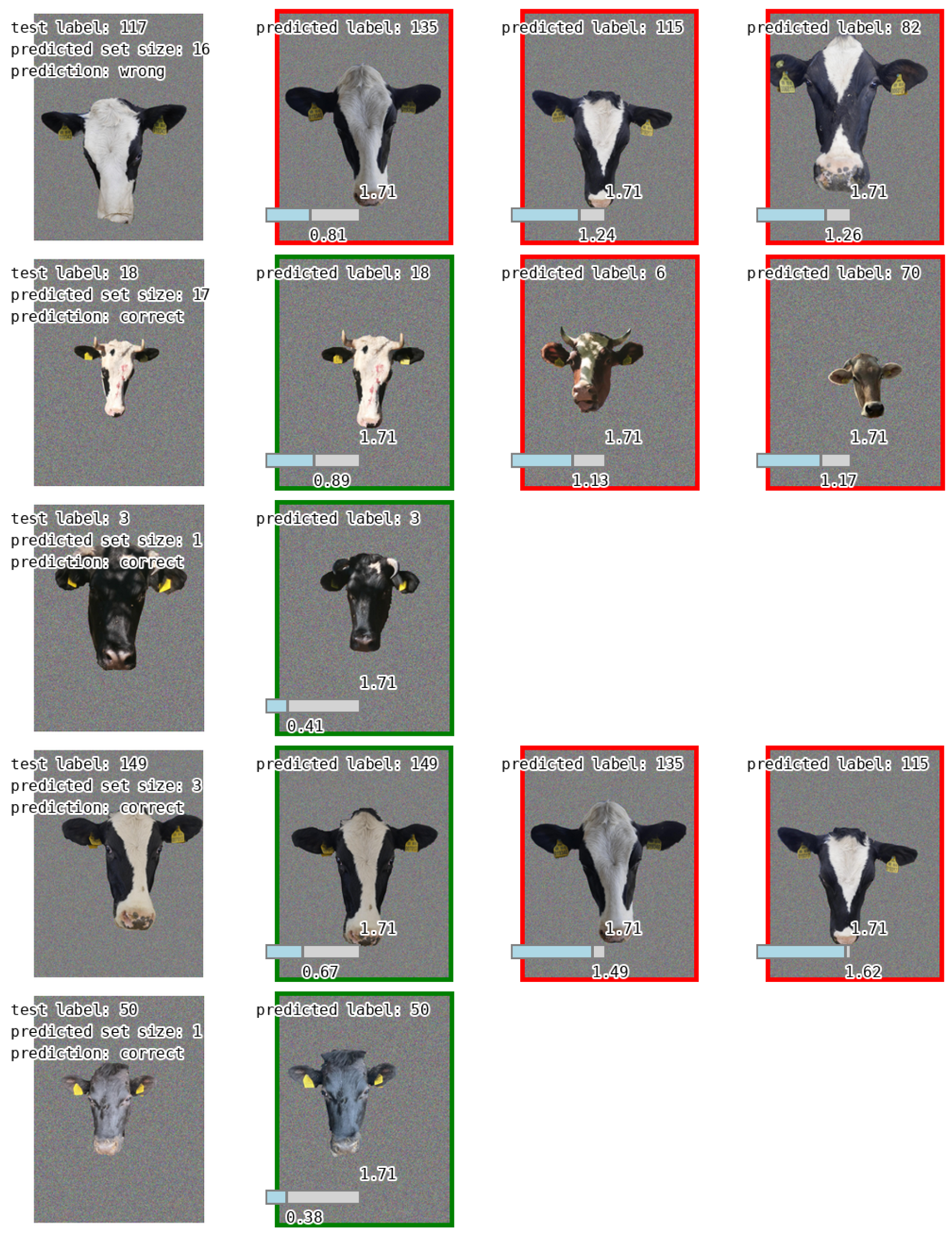
A practical illustration of the framework is the grid visualization in Figure 1. It shows conformal prediction sets for the cow dataset using ResNet-50 embeddings with the ${non}_{\mathrm{ratio}}$ scoring function at $q=0.8$. The prediction sets vary considerably in size: some test images yield singleton sets (containing only the true label), while others include multiple labels. Notably, approximately 18 out of 62 test images (29%) receive singleton prediction sets at this confidence level, indicating high embedding quality for those individuals. However, several test images exhibit large prediction sets spanning 20+ labels, suggesting ambiguity in the embedding space for those individuals. The wrong predictions with low nonconformity on the first and fourth rows display similar visual characteristics of the animals.

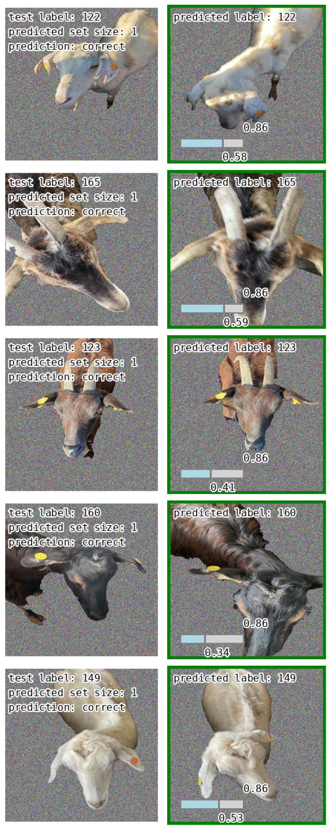
Similarly, Figure 2 shows the goat dataset with Swin-T embeddings and the same nonconformity function ${non}_{\mathrm{ratio}}$. Here, the embedding space provides much better separation—approximately 31 out of 36 test images (86%) receive singleton prediction sets at confidence level $q=0.8$, demonstrating the Swin-T model’s strong discriminative capability for this dataset. The few non-singleton sets typically contain only 2–3 labels, indicating minor ambiguity rather than systematic confusion.

The bar beneath each reference image visualizes the nonconformity score for that candidate label. The gray portion represents the quantile threshold ${\widehat{q}}_q$ (specifically ${\widehat{q}}_{0.8}$ for confidence level $q=0.8$) derived from the calibration set—this is the maximum score allowed for a label to be included in the prediction set at the chosen confidence level. The blue portion shows the actual nonconformity score for that specific label, relative to ${\widehat{q}}_q$. When the blue bar is shorter than the gray bar, the score is below the threshold and the label is included in the prediction set. The numeric value displayed below the bar shows the exact nonconformity score value, while ${\widehat{q}}_q$ is shown above the bar.

Each grid contains test images in the first column, annotated with the true label (test label), the size of the prediction set (predicted set size), and whether the true label is correctly included in the set (prediction: “correct” if the true label is in the prediction set, “wrong” otherwise). The subsequent columns display the predicted labels sorted by their nonconformity scores in ascending order, with a green frame indicating labels that match the true label and a red frame indicating incorrect predictions.

To interpret these grids, one should examine test images where the nonconformity scores for the correct class are substantially lower than the threshold (short blue bars), indicating high conformity. Conversely, test images where the correct class has a score near or above the threshold, or where incorrect classes exhibit notably lower scores, reveal cases of potential confusion or ambiguity in the embedding space.

Having examined individual prediction sets, the next aspect to consider is whether the conformal prediction framework achieves its theoretical calibration guarantees across different confidence levels.

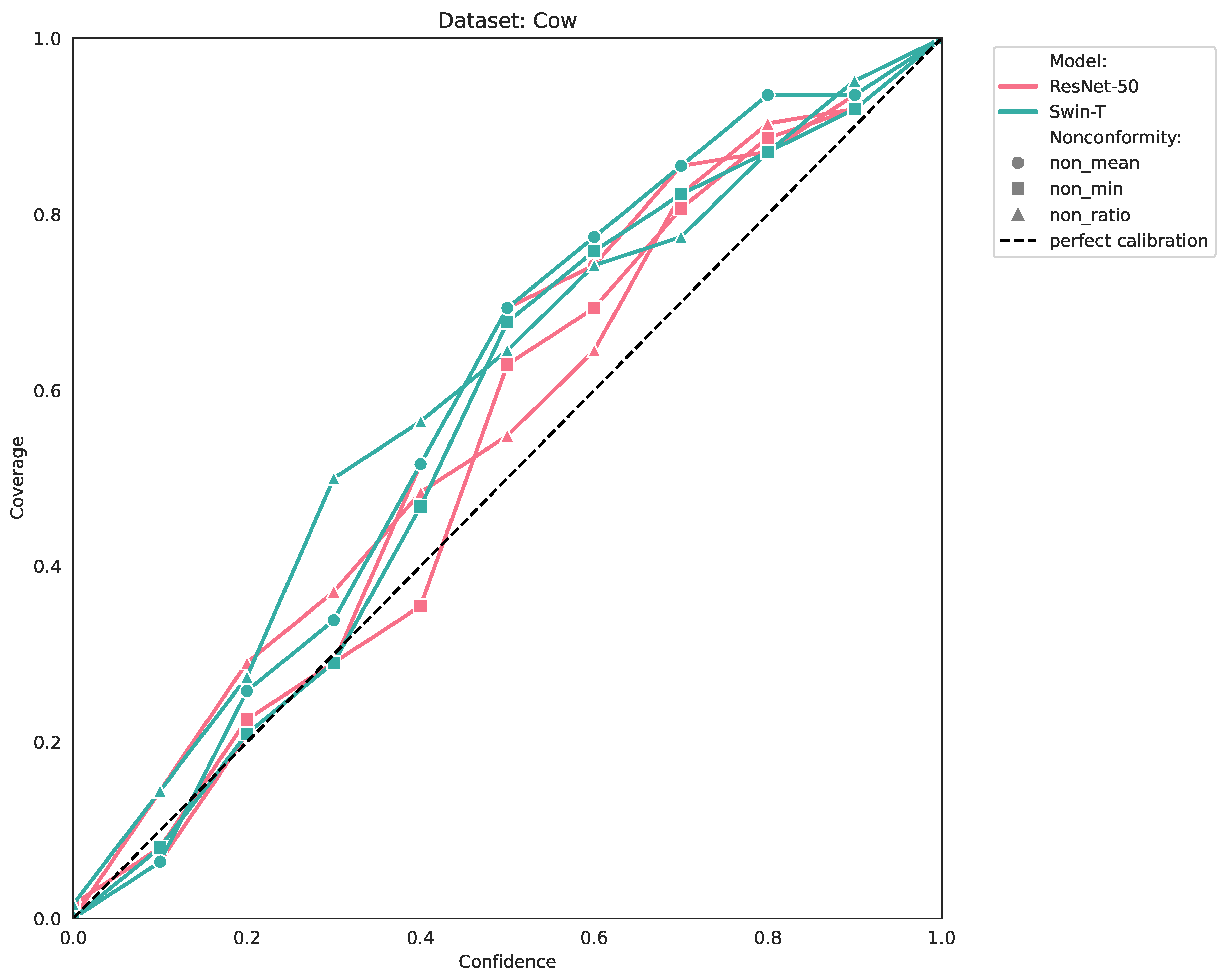
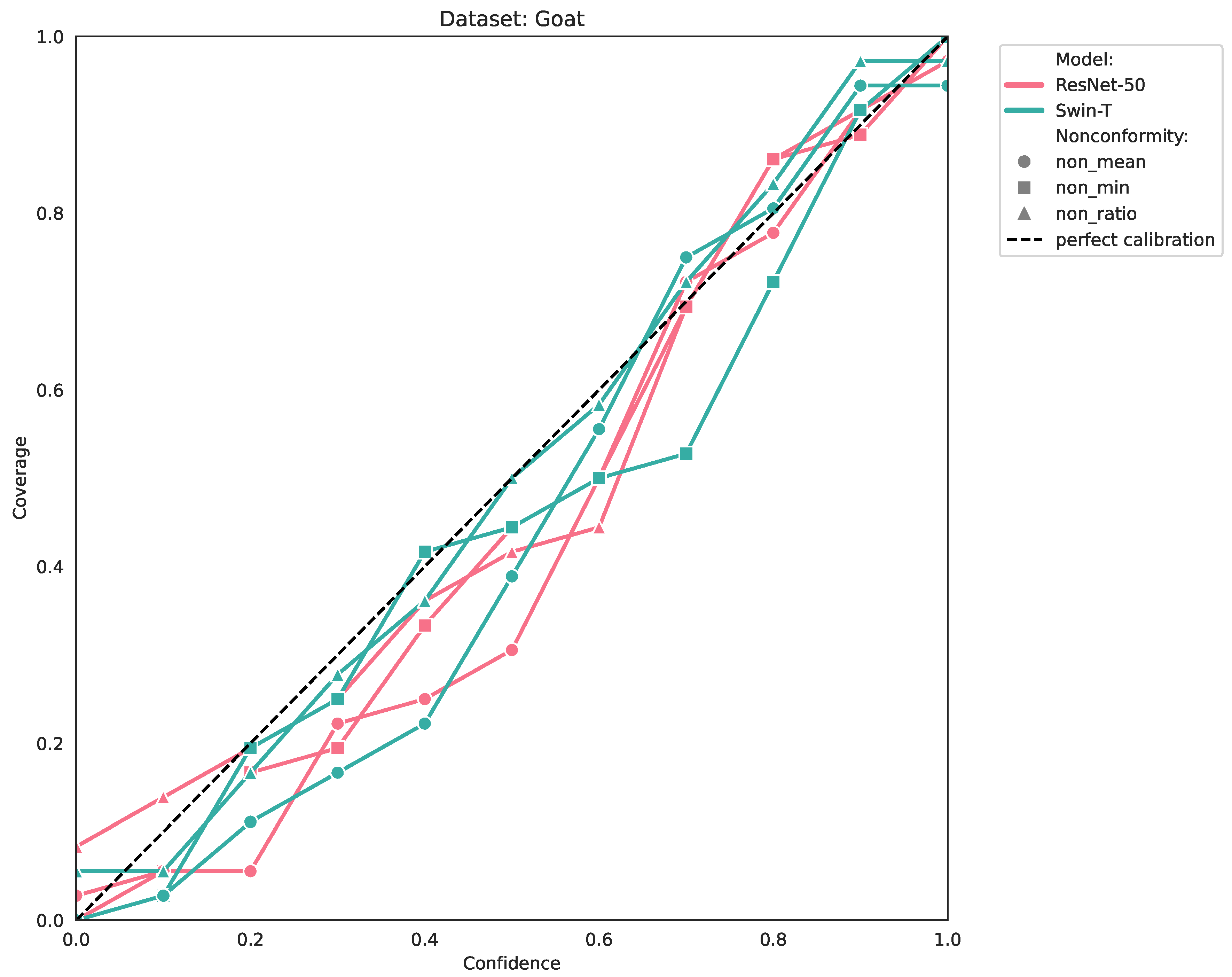
The coverage plots illustrate the calibration properties of the conformal prediction method across different confidence levels. In conformal prediction, calibration refers to the relationship between the user-specified confidence level (the desired probability that the true label is included in the prediction set) and the empirical coverage achieved on test data.

For the cow dataset (Figure 3), coverage at $q=0.8$ ranges from approximately 78% to 82% depending on the nonconformity measure, showing slight under-coverage (the predictor is slightly liberal). The ${non}_{\mathrm{ratio}}$ measure with ResNet-50 achieves 78.2% ± 7.9% coverage, while Swin-T with the same measure yields 79.5% ± 6.2%. The coverage is generally close to the desired level, with the gap narrowing at higher confidence levels.

The goat dataset (Figure 4) exhibits coverage at $q=0.8$, ranging from 76% to 86% depending on the model and nonconformity measure. The ${non}_{\mathrm{ratio}}$ measure with ResNet-50 achieves 85.8% ± 9.8% coverage, while Swin-T with the same measure reaches 78.9% ± 9.9%. The goat dataset shows more variation across nonconformity measures and across runs (standard deviations of 7–10 percentage points), with ${non}_{\mathrm{ratio}}$ producing the smallest prediction sets while maintaining valid coverage. The calibration curves are generally close to the diagonal, indicating reasonable calibration, though with some under-coverage at intermediate confidence levels for certain measure–architecture combinations. This variation is consistent with known finite-sample properties of split conformal prediction.

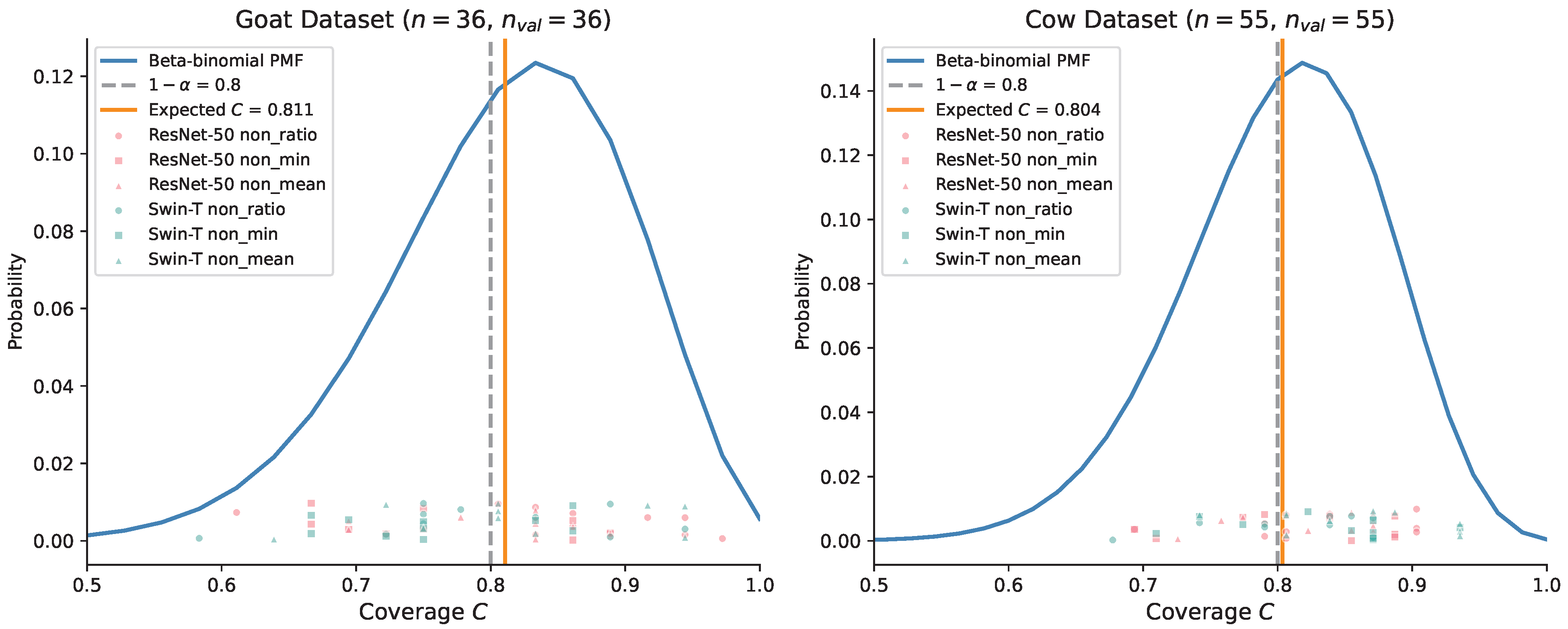
Figure 5 illustrates the theoretical beta-binomial distribution (Equation (7)) of coverage estimates for both datasets. The distribution is centered around the expected coverage (81.1% for goat, 87.3% for cow) but exhibits substantial spread due to finite sample sizes. The narrower distribution for the cow dataset reflects its larger calibration set size ($n=55$ versus $n=36$).

Note that the smaller size of the goat dataset leads to higher variance across runs, hence the standard deviations reported in Table 2. Although the datasets are relatively small, the use of repeated random splits and reporting of variability provides a more robust assessment of the conformal framework. This is particularly relevant under realistic small-data conditions typical in livestock applications. Future work with larger datasets would yield more stable estimates. This reflects the primary focus of the present study on controlled evaluation of conformal prediction in livestock identification settings rather than on benchmarking against large-scale public re-identification datasets.

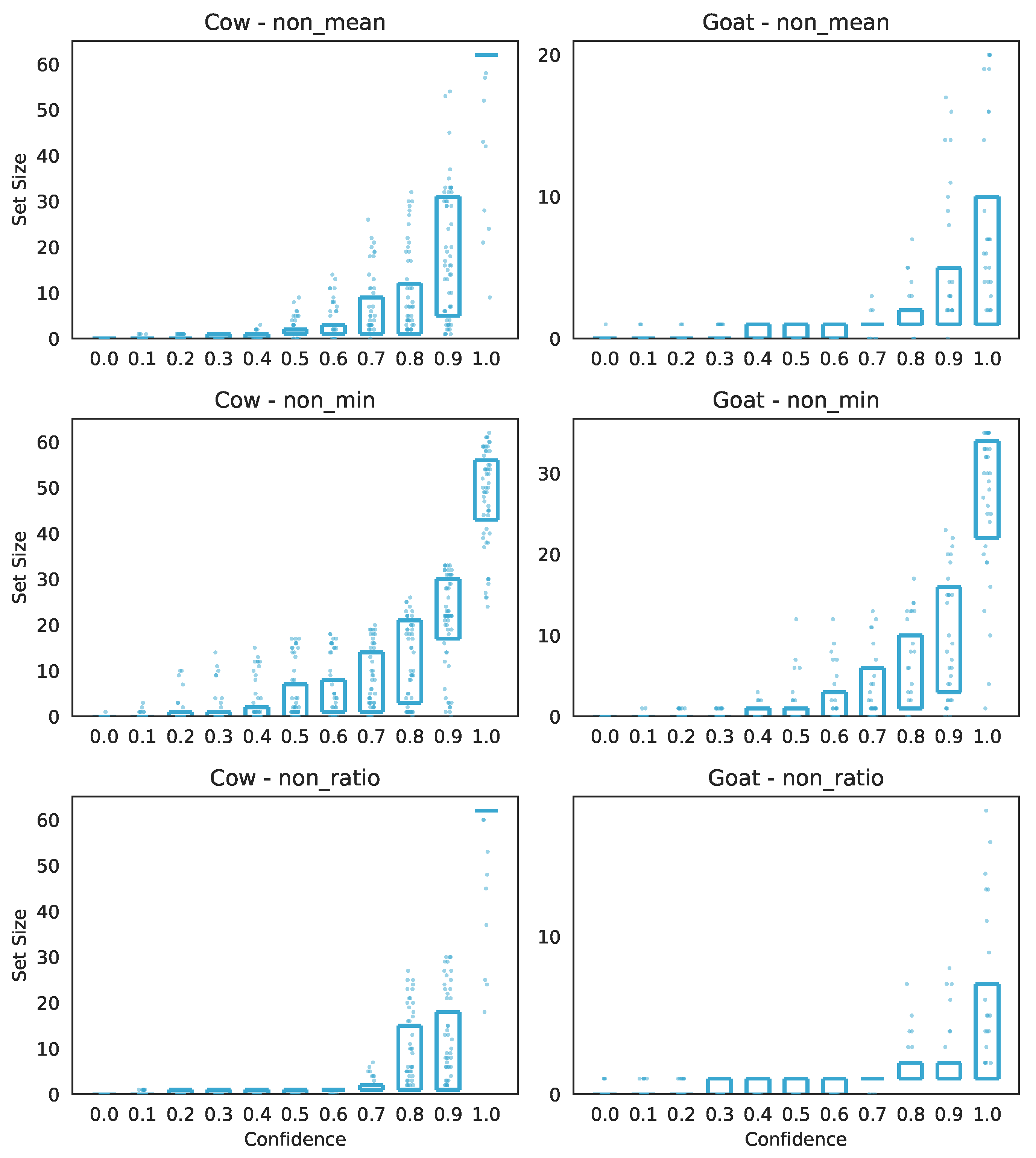
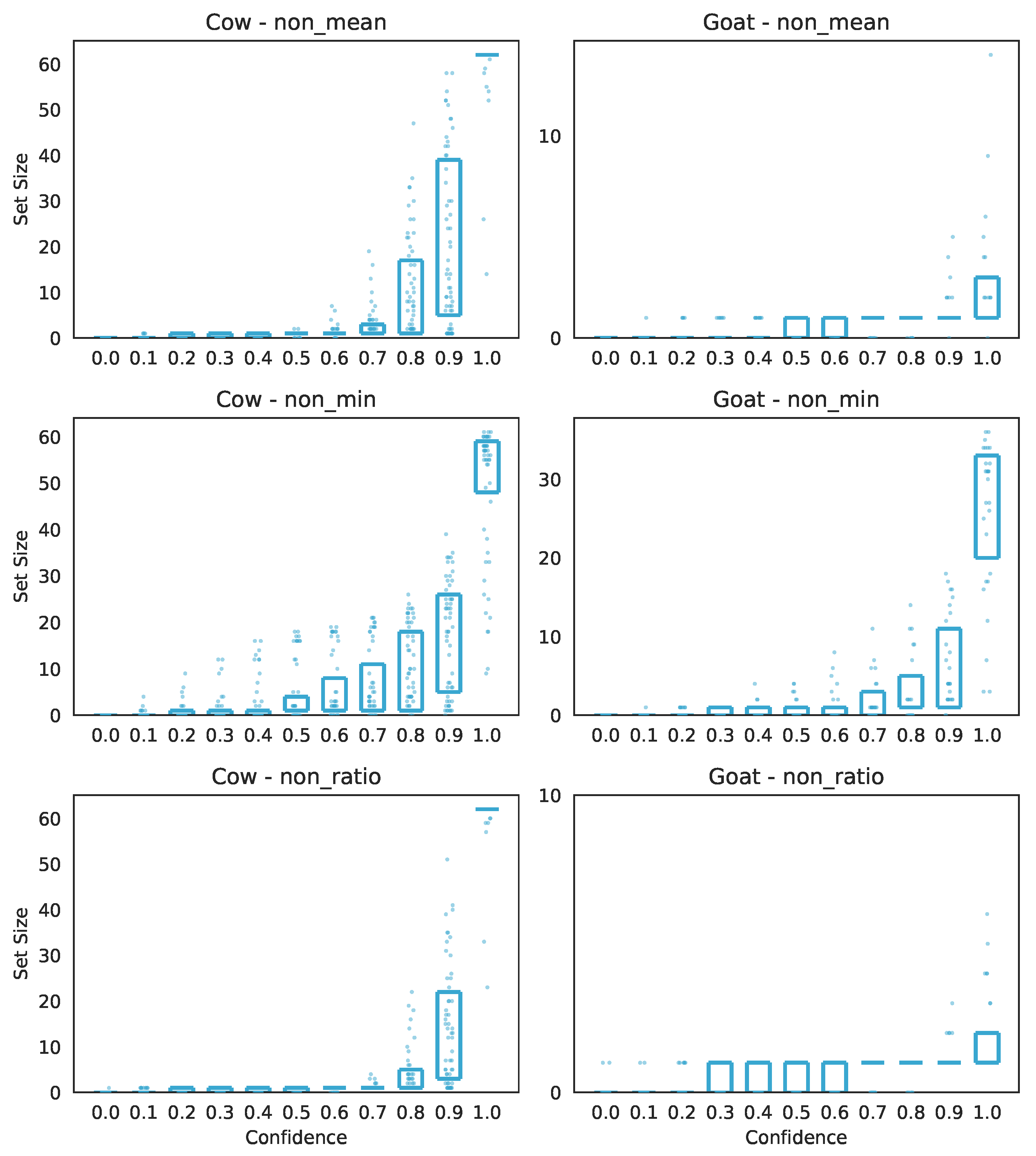
The set size distribution plots (Figure 6 and Figure 7) characterize the granularity of conformal prediction sets across different confidence levels for the ResNet-50 and Swin-T models, respectively. At $q=0.8$, the cow dataset shows a wide variance in prediction set sizes, with on average 37.2 ± 9.9 singleton sets for ResNet-50 and 45.6 ± 8.2 for Swin-T (with ${non}_{\mathrm{ratio}}$), with mean set sizes of 3.00 ± 1.78 and 1.84 ± 1.02, respectively. In contrast, the goat dataset exhibits much tighter prediction sets at the same confidence level, with on average 29.4 ± 2.9 singletons out of 36 test images for ResNet-50 and 28.9 ± 3.8 for Swin-T with ${non}_{\mathrm{ratio}}$, and mean set sizes under 1.2. The ${non}_{\min }$ measure produces larger and more variable set sizes compared to ${non}_{\mathrm{ratio}}$ for both datasets and models, reflecting its sensitivity to nearest-neighbor distances without the comparative normalization. The ${non}_{\mathrm{mean}}$ measure shows intermediate behavior, providing a balance between set compactness and coverage.

Figure 6 and Figure 7 aid the analysis of prediction set sizes. For the cow dataset with ResNet-50, it is evident from the first plot in the last row of Figure 6 that ${non}_{\mathrm{ratio}}$ gives the most confident predictions. The mean set size evolves as follows: at $q=0.0$, all prediction sets are empty (mean = 0.00) because the threshold corresponds to the minimum nonconformity score on the calibration dataset, which very few labels can satisfy. As q increases to 0.1–0.5, the mean set size grows gradually from 0.15 to 0.63, with singleton sets (containing exactly one label) becoming predominant. At $q=0.5$, 39 out of 62 test images receive singleton sets. The inflection point occurs between $q=0.6$ and $q=0.7$, where the rate of mean set size increase jumps from 2.10 per 0.1 increment to 8.06 per 0.1 increment. The most dramatic expansion happens at $q=0.8$, where the mean set size jumps to 7.90 with a rate of 62.58 per 0.1 increment, and the standard deviation reaches 8.27—indicating extreme heterogeneity in prediction set sizes across test images. By $q=0.9$, the mean reaches 10.35, and at $q=1.0$, the mean set size approaches the full label space (58.97 out of 62 possible labels), as the threshold becomes the maximum calibration score.

Equivalent patterns emerge when examining the Swin-T model, though with notably different scale characteristics, as shown in Figure 7.

The inflection point analysis in

Table 3. Inflection point analysis for the foreground-only variants: confidence level q where mean set size first exceeds 3 labels.

Dataset	Model	Measure	Inflection q
Cow	ResNet-50	${non}_{\mathrm{ratio}}$	0.9
Cow	ResNet-50	${non}_{\min }$	0.6
Cow	ResNet-50	${non}_{\mathrm{mean}}$	0.7
Cow	Swin-T	${non}_{\mathrm{ratio}}$	0.9
Cow	Swin-T	${non}_{\min }$	0.6
Cow	Swin-T	${non}_{\mathrm{mean}}$	0.8
Goat	ResNet-50	${non}_{\mathrm{ratio}}$	1.0
Goat	ResNet-50	${non}_{\min }$	0.7
Goat	ResNet-50	${non}_{\mathrm{mean}}$	0.9
Goat	Swin-T	${non}_{\mathrm{ratio}}$	1.0
Goat	Swin-T	${non}_{\min }$	0.8
Goat	Swin-T	${non}_{\mathrm{mean}}$	1.0

reveals when the dramatic set size expansion begins for each configuration. A later inflection point indicates more robust embeddings where uncertainty remains controlled at higher confidence levels.

The results show that the ratio-based nonconformity score produces the most efficient prediction sets while maintaining empirical coverage close to the desired confidence level across both datasets and embedding models.

4. Discussion

We note that alternative uncertainty estimation approaches such as distance thresholding and Bayesian methods (e.g., MC dropout) are commonly used. The goal of this work is not to outperform such methods in accuracy but to demonstrate that conformal prediction provides a complementary framework with formal coverage guarantees. Beyond the coverage guarantees, analyzing prediction set sizes provides insights into the practical behavior of the conformal prediction framework.

This non-monotonic behavior in variance is particularly informative: at low confidence levels ($q<0.5$), most prediction sets are either empty or singletons, reflecting that the threshold is so strict that only the most confident labels pass. At intermediate confidence ($q\approx 0.5$–0.7), a sweet spot emerges where approximately 70–85% of test images receive singleton sets while maintaining valid coverage. Beyond this sweet spot ($q>0.8$), the prediction sets explode in size as the threshold admits increasingly atypical labels, eventually encompassing nearly all candidates at $q=1.0$. Qualitative inspection indicates that larger prediction sets typically arise for visually similar individuals or low-quality images (e.g., occlusion, motion blur). These cases highlight the sensitivity of embedding-based identification to fine-grained visual similarity and suggest that conformal prediction appropriately reflects ambiguity in such scenarios.

The experiments indicate that moderate confidence levels often provide the most useful operational trade-off. Very high confidence levels substantially increase the size of the prediction sets, particularly for more challenging datasets such as cattle. The improved performance on the goat dataset may be related to greater visual variability across individuals, which can facilitate discrimination in embedding space. The cow dataset appears to contain more visually similar subjects. Consequently, in practical livestock monitoring systems, confidence levels may be selected based on the acceptable balance between decision certainty and operational efficiency. In practical deployment, segmentation can be automated using pretrained instance segmentation models (e.g., Mask R-CNN or YOLO-based segmentation), eliminating the need for manual annotation.

A notable feature of conformal prediction is the ability to identify uncertain or out-of-distribution examples through credibility. The credibility of an example x is defined as the smallest q for which the prediction set is not empty. The rationale behind this definition is that the model prefers to make a known wrong prediction (the empty set) instead of adding any labels that appear too distant. If the confidence for such a known wrong prediction is high, then none of the known labels are better than this at that confidence level [29]. Although credibility analysis was not applied in the current experiments, extending the framework to report credibility scores should be straightforward.

The dataset difficulty fundamentally shapes this trend. For the goat dataset, the identification task proves substantially easier: at $q=0.8$, the mean set size is only 1.16 ± 0.28 for ResNet-50 (versus 3.00 ± 1.78 for cow), with approximately 82% singleton sets on average. The inflection point is far less dramatic—the set size increases smoothly from near 0 at $q=0.0$ to around 1–2 at high confidence levels, never experiencing the explosive growth observed for cow identification. This indicates that both models provide excellent separation for goat individuals.

The choice of nonconformity measure substantially modulates the trend. At $q=0.8$, comparing the three measures for cow with ResNet-50: ${non}_{\mathrm{ratio}}$ yields mean = 3.00 ± 1.78 with 37.2 ± 9.9 singletons, ${non}_{\mathrm{mean}}$ yields mean = 5.91 ± 1.46 with 23.0 ± 4.4 singletons, while ${non}_{\min }$ produces mean = 8.96 ± 2.35 with only 12.9 ± 2.0 singletons—nearly double the average set size of ${non}_{\mathrm{ratio}}$. The ${non}_{\min }$ measure exhibits higher variance at every confidence level because it lacks the comparative normalization that ${non}_{\mathrm{ratio}}$ and ${non}_{\mathrm{mean}}$ provide via the denominator (distance to nearest competitor). This confirms that ratio-based measures offer superior efficiency for this identification task.

The feature extractor also influences the trend shape. Swin-T achieves approximately 74% singleton sets at $q=0.8$ for cow (versus 60% for ResNet-50, averaged over 10 runs), with a mean set size of 1.84 ± 1.02 (versus 3.00 ± 1.78). The Swin-T inflection point is also delayed—the dramatic expansion begins at $q=0.9$ for ${non}_{\mathrm{ratio}}$—indicating that Swin-T embeddings provide more consistent separation across individuals, pushing the uncertainty threshold further toward the maximum calibration score.

Based on the results from the previous section, the optimal configuration for conformal prediction in animal identification is Swin-T with ${non}_{\mathrm{ratio}}$: it achieves the highest singleton rates (80–90% on average), lowest mean set sizes (0.80 ± 0.11), and maintains valid coverage above 80%. For practitioners requiring the tightest prediction sets, targeting $q=0.7$ with Swin-T and ${non}_{\mathrm{ratio}}$ provides an excellent trade-off, yielding 56–86% singleton sets while maintaining 77–82% empirical coverage.

The split conformal prediction framework assumes a fixed calibration set from which thresholds are computed once before deployment. Several practical extensions could address this limitation in future work. Online conformal prediction methods [32] could enable dynamic calibration as new animals enter the system, though the online setting requires validation. Similarly, approximate nearest-neighbor search with FAISS [33] could improve computational efficiency for large-scale deployment but has not been tested. The credibility score conceptually enables anomaly alerting in farm settings, but this application requires experimental evaluation. These directions are mentioned as potential improvements rather than claims supported by the present experiments.

5. Conclusions

This paper demonstrates the practical application of conformal prediction to animal identification using pretrained neural network embeddings. Experiments on cow and goat datasets with ResNet-50 and Swin-T show empirical coverage behavior consistent with the conformal prediction framework; the ${non}_{\mathrm{ratio}}$ measure consistently produces the smallest prediction sets while maintaining valid coverage, and Swin-T achieves tighter prediction sets (80–90% singletons on average at $q=0.8$) than ResNet-50 (60–80% singletons on average).

The conformal framework provides a principled mechanism for uncertainty quantification in identification tasks, producing candidate sets rather than single labels. This is particularly valuable in agricultural settings: when the prediction set contains multiple candidates, it can be presented to a farmer or veterinarian for final decision-making; high-confidence cases (singleton sets) can be automatically processed; and uncertain cases can be flagged for manual review. The distribution-free coverage guarantees ensure reliable performance without requiring assumptions about the underlying data distribution.

Limitations of the proposed method include the requirement for a separate calibration set and the provision of marginal (rather than conditional) coverage guarantees. Prediction set size can be substantial for challenging datasets.

Several directions could strengthen this work: extending to online conformal prediction for dynamic farm environments, investigating conditional coverage guarantees for specific subgroups, and exploring adaptive methods that adjust based on test example characteristics.