Article

Analysis of the Impact of Doppler Frequency Shift on Phase Noise in Space-Borne Gravitational Wave Detection


1
MOE Key Laboratory of TianQin Mission, TianQin Research Center for Gravitational Physics, School of Physics and Astronomy, Sun Yat-sen University (Zhuhai Campus), Zhuhai 519082, China
2
School of Electronics and Communication Engineering, Sun Yat-sen University, Shenzhen 518000, China
*
Author to whom correspondence should be addressed.
Technologies 2026, 14(3), 160; https://doi.org/10.3390/technologies14030160
Submission received: 27 January 2026 / Revised: 24 February 2026 / Accepted: 3 March 2026 / Published: 4 March 2026
(This article belongs to the Section Information and Communication Technologies)

Abstract

Space gravitational wave detection is performed via a laser interferometry system across hundreds of thousands to millions of kilometers for picometer-level displacement measurement, using phasemeters to read gravitational wave-induced displacement changes. A critical yet unresolved challenge is the coupling of Doppler frequency shift—resulting from relative satellite motion—into the phase measurements, as well as its consequent impact. To address this, we analyzed the Doppler effect principle, built a laser interferometry signal model, and obtained signal frequency ranges via orbit simulation. We then conducted time- and frequency-domain analyses of the phasemeter, theoretically deriving steady-state phase errors to clarify how Doppler shift affects phasemeter noise. A hardware system was constructed for verification, showing that phase noise curves rise significantly at a 100 Hz/s Doppler shift rate, and increasing phasemeter bandwidth increases low-frequency phase noise. This study provides a theoretical and experimental basis for phasemeter parameter optimization and ground experiments of phasemeters in space gravitational wave detection.

1. Introduction

In 1915, Einstein proposed the theory of general relativity and predicted the existence of gravitational waves based on it [1]. However, at that time, the existence of gravitational waves had not yet been confirmed, and doubts were expressed about their physical authenticity. The first direct detection of gravitational waves occurred in 2015, when the first gravitational wave event, GW150914, was detected by the Laser Interferometer Gravitational Wave Observatory (LIGO) in the United States. However, it caused a strain equivalent to an atomic-scale displacement over the Earth’s diameter for accuracy and clarity, making the detection of gravitational waves very difficult. Due to the extremely weak interaction between gravitational waves and matter, gravitational waves propagate almost without attenuation in the universe [2]. By detecting gravitational waves, we can gain a better understanding of the properties of black holes [3] and neutron stars [4], the structure of the universe [5], and even the properties of gravity itself [6].
The design purpose of the TianQin Project [7] is to achieve gravitational wave detection in the frequency range of 0.1 mHz–1 Hz. To this end, TianQin plans to deploy three identical satellites around 100,000 km in Earth’s orbit around 2035 to form an equilateral triangular constellation with an arm length of 170,000 km, therefore building a space gravitational wave observatory. TianQin will adopt a “3 + 3” mode, which means a three-month rest and three-month detection mode, detecting gravitational waves in an orbit without lunar shadows for six months each year [8]. The normal direction of the TianQin satellite’s orbital plane is selected to point towards RX J0806.3 + 1527. By using responsive intersatellite laser interferometry measurement technology, the phase changes in laser propagation between test masses are accurately measured to obtain information on the changes in laser path length, thereby achieving the purpose of measuring gravitational waves. The TianQin Plan requires that the displacement measurement noise within the measurement frequency band should not exceed 1 pm/ Hz [9], and the phase noise allocated to the phasemeter should not exceed 1 μ rad / Hz .
Such stringent accuracy requirements make traditional phase measurement techniques, including zero-crossing phase detection [10], correlation function method [11], and in-phase/quadrature (I/Q) demodulation [12], inadequate. To address this, Ware et al. [13] proposed a novel Phase Measurement System (PMS), also known as a phasemeter, in 2006. This system employs a Digital Phase Locked Loop (DPLL) to directly track the frequency variations in the input signal. However, analog frequency division tests have shown that the performance of the PMS is limited by the jitter noise of the Analog-to-Digital Converter (ADC), which can significantly degrade performance at high input frequencies. Subsequently, Gerberding et al. [14] proposed an accurate ADPLL model and implemented a multi-channel PMS on a Field-Programmable Gate Array (FPGA). As a digital circuit, the ADPLL exhibits low sensitivity to power supply noise, substrate noise, and parasitic effects, which are factors that typically affect the performance of phase-locked loops. Furthermore, the digital architecture offers high scalability on FPGAs. This architecture meets the requirements for multi-channel, high-speed, and high-precision PMS in space-borne gravitational wave detection. The ADPLL-based phasemeter system has now passed performance verification under LISA conditions [15] and has been successfully applied to the Laser Ranging Interferometer (LRI) of the Grace follow-up mission [16].
The orbit of the TianQin constellation is actually unstable, and there is relative motion between the satellites [17]. Relative motion introduces a Doppler shift. When the Doppler shift varies widely, the carrier frequency of the beat signal will inevitably fluctuate widely as well. To prevent the laser beat frequency from exceeding the receiving range of the optical detector, LISA has implemented a laser frequency offset plan for such situations [18]. LISA studied the update cycle of the delay-locked loop and the time error caused by the Doppler effect [19]. Theoretical analysis shows that the Doppler effect has little impact on the locking and tracking of pseudo-code in the delay-locked loop. In the TianQin project, Zheng Lu investigated the impact of the Doppler effect on time interferometry [20]. The TDI algorithm cannot eliminate the Doppler effect and can only filter out frequencies below 10−4 Hz through a high-pass filter. Huang Xiangqing discussed that Doppler frequency shift can affect sampling jitter noise [21]. In the Taiji project, Minghui Du discussed high-fidelity simulations of space-borne gravitational wave antenna under the influence of a Doppler shift between SCs within ±5 MHz [22].
In general, due to the stringent requirements for phase measurement accuracy in space gravitational wave detection, ignoring the impact of Doppler frequency shift variations on phase noise in the phasemeter may well lead to the failure of space-borne gravitational wave detection missions. Therefore, this paper first models the laser interferometric displacement measurement signal affected by the Doppler effect and simulates the Doppler frequency shift experienced by satellites through software. Subsequently, we explore the impact mechanism from both time-domain and frequency-domain perspectives. The theoretical analysis shows that Doppler frequency shift leads to steady-state phase errors, which in turn affect phase noise. Finally, the conclusion that Doppler frequency shift affects phase noise is confirmed through hardware experiments.

2. Modeling and Simulation of Laser Interferometric Displacement Measurement Signal Under Doppler Frequency Shift

2.1. Doppler Frequency Shift Principle

Due to the relative motion of inter-satellite orbits, the two satellites have a relative velocity in the direction of the line of sight. Therefore, when the laser is transmitted from the transmitting end to the receiving end, under the Doppler effect of special relativity, the frequency at the receiving end f R and the frequency at the transmitting end f T can be expressed as:
f R = f T c v c + v = k f T
In the formula, c represents the speed of light, v denotes the relative velocity in the line-of-sight direction between two satellites, v > 0 indicates that the two satellites are moving away from each other, and k represents the Doppler coefficient.
The Doppler shift f D can be expressed as:
f D = f T f R = ( 1 k ) f T v c f T ,
since v c , the first-order Taylor expansion approximation is valid, yields f D v c f T .
Assuming the time-domain signal at the transmitting end x T ( t ) and the frequency-domain signal is X T ( f T ) , the frequency-domain signal at the receiving end is X R ( f R ) ; thus, we have:
t = t k ,
X R ( f R ) = F [ x ( t ) ] = k X T ( k f T ) = k X T ( f T + f D )
From the above formula, it can be seen that the time of the signal at the receiving end becomes 1 k times that at the transmitting end in the time domain, while in the frequency domain, it shifts leftward by f D as a whole and its amplitude is enlarged to k times that at the receiving end.

2.2. Laser Interferometric Displacement Measurement Signal Modeling

The schematic diagram of laser interferometric displacement measurement is shown in Figure 1, from which it can be seen that two satellites (Satellite 1 and Satellite 2) are equipped with independent laser sources (Laser 1 and Laser 2), respectively. In measurement mode, the lasers on Satellite 1 and Satellite 2 emit laser light, which is modulated by an electro-optic modulator (EOM) to modulate clock noise and pseudo-code phase for subsequent ground TDI processing, resulting in laser S 1 and laser S 2 . The laser is detected by the quadrant photodetector (QPD), conducted using Signal Conditioning Electronics (SCEs), and then enters the Analog-to-Digital Converter (ADC) for subsequent laser phase measurements.
Laser S 1 and laser S 2 can be expressed in a formula:
S 1 = E e i [ 2 π f 1 t + m s b cos ( 2 π f M 1 t + ϕ U S O 1 ) + m p r n p 1 ( t ) ] ,
S 2 = E e i [ 2 π f 2 t + m s b cos ( 2 π f M 2 t + ϕ U S O 2 ) + m p r n p 2 ( t ) ]
In the formula, f 1 and f 2 represent the initial frequency of the laser, f M 1 and f M 2 represent the clock noise frequency, ϕ U S O 1 and ϕ U S O 2 represents the initial phase of ultra-stable oscillator, E represents the amplitude emitted by the laser, m s b represents the modulation index of the side frequency, m p r n represents the phase modulation depth of the pseudo-code, and p 1 ( t ) and p 2 ( t ) denote the pseudo-code information.
Laser S 1 propagates through Satellite 1’s optical bench, is expanded by Satellite 1’s telescope and sent to Satellite 2, received by Satellite 2’s telescope, reflected by the test mass (TM) on Satellite 2, and interferes with Laser 2 through the optical bench. The propagated lasers are denoted as S 1 and S 2 , φ 1 and φ 2 indicating the phase changes caused by the laser passing through different distances, where E S is received light amplitude, and E L O is local satellite light amplitude. So the lasers can be expressed as:
S 1 = E S e i [ 2 π f 1 t + φ 1 + m p r n p 1 ( t ) ] e i [ m s b cos ( f M 1 t + ϕ U S O 1 ) ] ,
S 2 = E L O e i [ 2 π f 2 t + φ 2 + m p r n p 2 ( t ) ] e i [ m s b cos ( 2 π f M 2 t + ϕ U S O 2 ) ]
The interference of signals with the same vibration direction is equivalent to the superposition of two waves, so:
S 12 = S 1 + S 2 ,
and the signal power can be expressed as:
P = S 12 S 12 *
The beat signal consists of one main beat signal and upper and lower clock sideband signals. After considering the Doppler shift, the main beat signal frequency and clock sideband frequencies both add 1 times the Doppler shift, because the laser signal only passes through one arm-length path. If considering laser 2 after weak light phase-locking propagating to Satellite 1 for beating, 2 times the Doppler shift needs to be added. Let Δ f = f 1 f 2 , φ 12 = φ 1 φ 2 , Δ f M = f M 1 f M 2 , f D = k f 1 f 1 = k f M 1 f M 1 , φ u p = φ 12 + m p r n p ( k t ) p ( t ) + ( φ U S O 1 φ U S O 2 ) , φ d o w n = φ 12 + m p r n p ( k t ) p ( t ) ( φ U S O 1 φ U S O 2 ) ; then, the beat signal can be modeled as:
P = P S + P L O + 2 P S P L O J 0 2 ( m s b ) cos 2 π ( Δ f + 2 f D ) t + φ 12 + m p r n p 1 ( k t ) p 2 ( t ) + 2 P S P L O J 1 2 ( m s b ) cos 2 π ( Δ f + 2 f D + Δ f M ) t + φ u p + 2 P S P L O J 1 2 ( m s b ) cos 2 π ( Δ f + 2 f D + Δ f M ) t + φ d o w n

2.3. TianQin Satellite Doppler Shift Simulation Analysis

The TianQin constellation orbit consists of three satellites with orbital radii of approximately 100,000 km, forming an equilateral triangle. The six orbital elements of the three satellites are shown in Table 1.
This study employs STK (Satellite Tool Kit) for satellite orbit simulation. The parameters are shown in Table 1. The STK step is 600 s, and the time span is 22 May 2034 to 22 May 2039, i.e., the satellite’s five-year operational life. And after sensitivity analysis (see Appendix A), it was found that a step size of 600 s is feasible.
For SC1, SC2 and SC3, the HPOP (High-Precision Orbit Propagator) model is selected here, incorporating gravitational perturbations from all planets in the solar system. STK considers orbital perturbations comprehensively; in STK’s HPOP, a complete set of high-fidelity dynamical models is used. The arm length between two satellites is calculated as:
L = r 1 r 2 ,
where L is the arm length between the two satellites and r 1 , r 2 represent the position coordinates of Satellite 1 and Satellite 2 in the J2000 coordinate system. The relative velocity in the line-of-sight direction is calculated as:
v 12 = L ˙ = e ^ 12 ( r ˙ 2 r ˙ 1 ) ,
e ^ 12 = ( r 1 r 2 ) L ,
where e ^ represents the unit vector. Additionally, ν is the laser frequency and the Doppler shift can be expressed as:
f D = v 12 c ν
Then, calculate the relative acceleration in the direction of the line of sight, as this data determines the rate of change in Doppler shift:
a 12 = L ¨ = e ^ 12 ( r ¨ 2 r ¨ 1 ) + 1 L ( r ˙ 2 r ˙ 2 L ˙ 2 ) ,
r a t e 12 = a 12 c υ
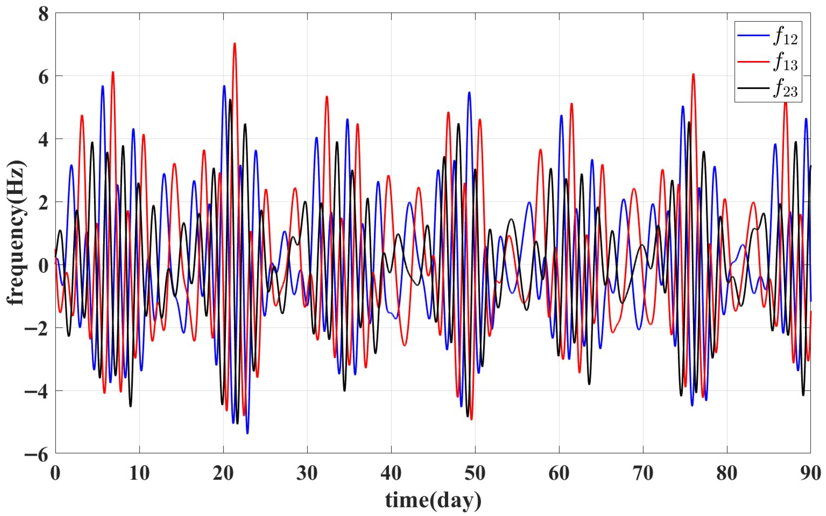
Through the STK simulation model results, as shown in Figure 2, within 90 days of satellite operation, considering double Doppler shift, the three groups of Doppler shifts between SC1, SC2, and SC3 pairs show a maximum Doppler shift range of −6 to 8 MHz. TianQin’s initial carrier center frequency is 10 MHz; considering the Doppler shift, the carrier center frequency fluctuates in the 4–18 MHz range, and considering 1 MHz upper and lower sidebands, TianQin’s beat signal frequency distribution range is 3–19 MHz.
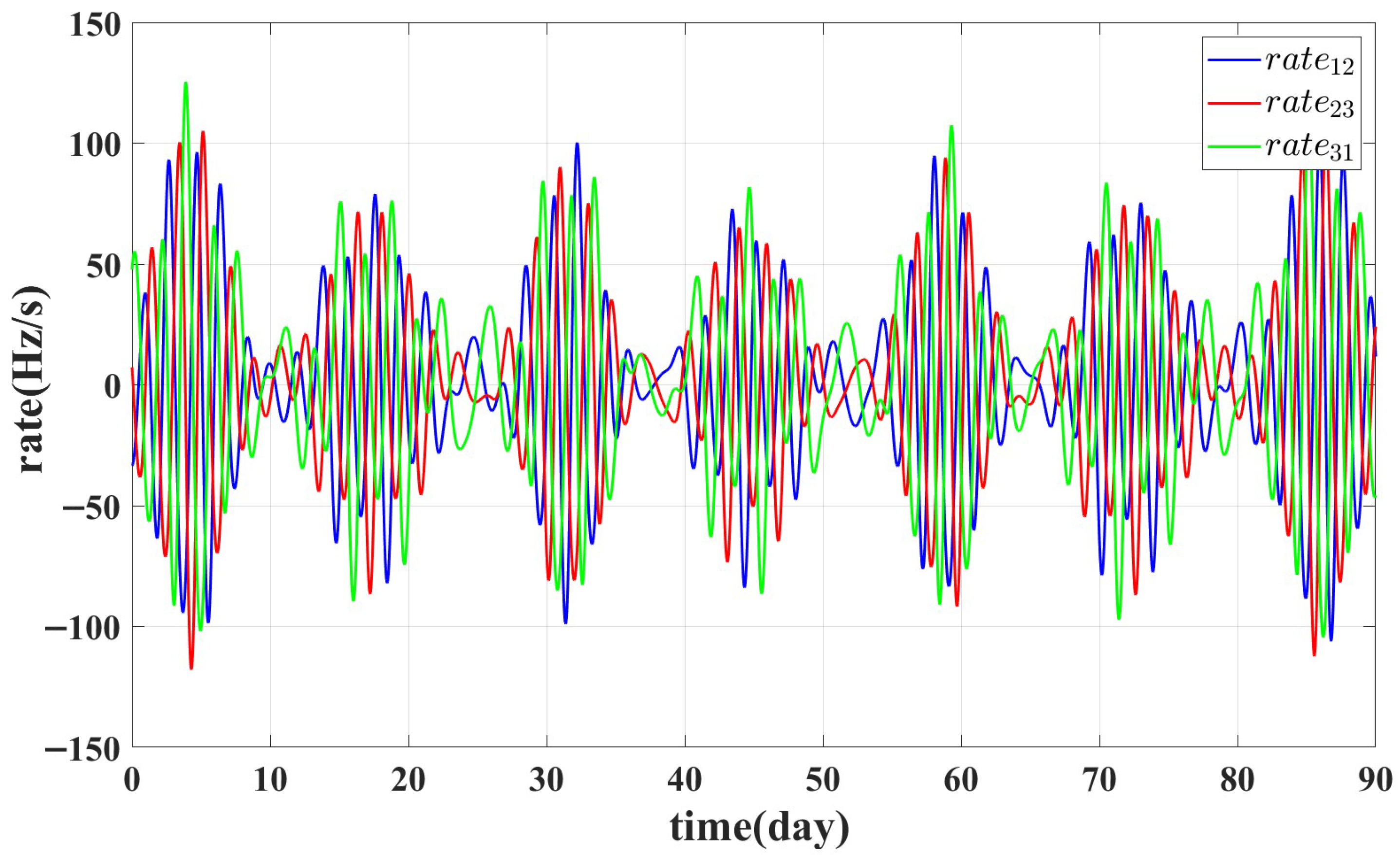
According to Formulas (16) and (17), we can simulate and obtain the Doppler shift rate results as shown in Figure 3; it can be observed that during the 90-day observation period of the satellite, the maximum rate is around 100 Hz/s.

3. Analysis of the Influence Mechanism of Doppler Shift on Phasemeter Noise

3.1. Time-Domain Analysis of Phasemeter System

The laser reflected back after weak light phase-locking from the far end interferes with the local satellite to form a beat, received by a quadrant photodetector (QPD), and the obtained main beat signal serves as the input to the phasemeter.
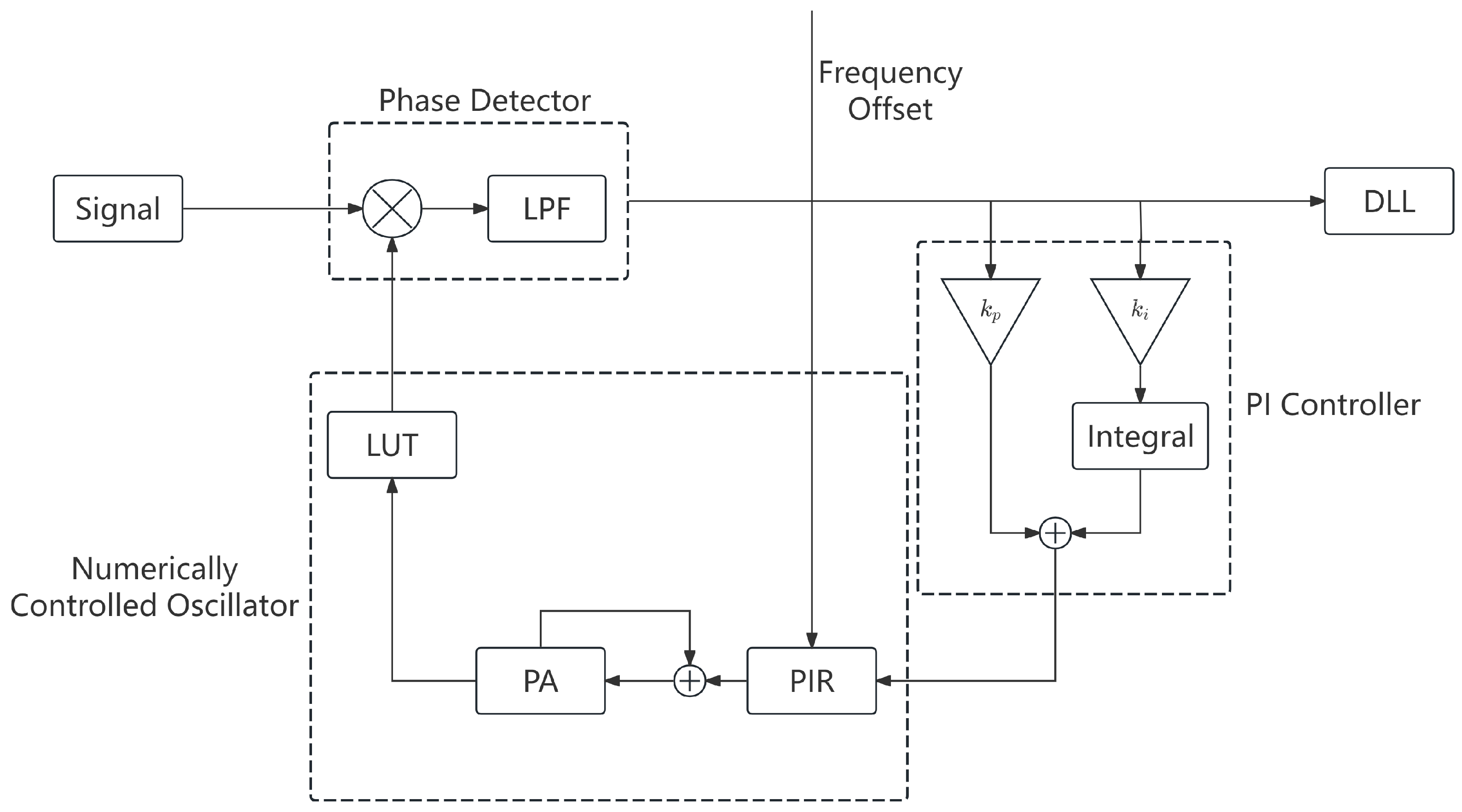
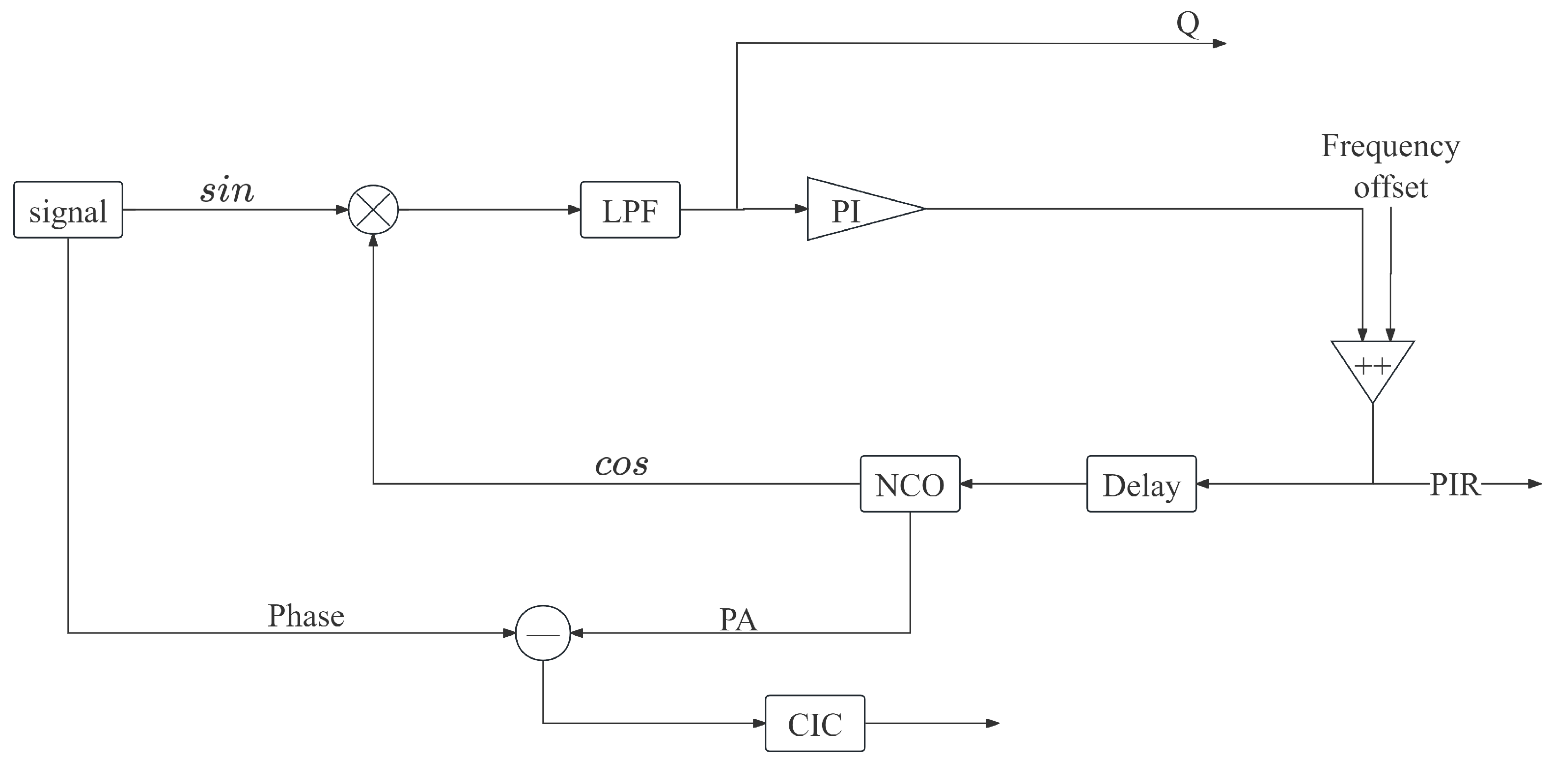
The phasemeter model can be represented as shown in Figure 4 above, mainly consisting of a phase detector, numerically controlled oscillator (NCO), and loop filter. The phase detector includes a multiplier and a low-pass filter (LPF); the loop filter is a PI loop controller, adjusting loop parameters to adjust loop bandwidth. The NCO includes a phase increment register (PIR), phase accumulator (PA), and cosine lookup table (LUT). We usually use the FFT module to calculate the frequency offset value and input it into PIR. Its purpose is to accurately track the beat signal from the ADC. The phasemeter’s main role is to read out the phase of the beat signal and output the Q-path signal as input for the subsequent DLL for absolute distance measurement.
From Formula (11), where A represents the main beat amplitude, denoting t as t , we get:
s i ( t ) = A cos 2 π ( Δ f + f D ) t + φ 12 + m p r n p 1 ( k t ) p 2 ( t ) ,
where f D represents all Doppler shifts.
Here, k is very close to 1, so approximate it as 1, denote 2 π ( Δ f + f D ) as ω i , and denote m p r n p 1 ( k t ) p 2 ( t ) as φ p r n ( t ) ; then, the equation becomes:
s i ( t ) = A cos ω i t + φ 12 + φ p r n ( t )
The phase can be expressed as:
θ i ( t ) = ω i t + φ 12 + φ p r n ( t )
The phase detector has two input signals: one is the main beat signal and the other is the quadrature reference signal output by the NCO. The initial NCO output is the sine value of the reference frequency ω c determined by the frequency offset:
s c ( t ) = sin ( ω c t )
After the multiplier, the signal is:
s m ( t ) = s i ( t ) s c ( t ) = A cos ω i t + φ 12 + φ prn ( t ) sin ( ω c t ) = A 2 [ sin ω i t + φ 12 + φ prn ( t ) + ω c t sin ω i t + φ 12 + φ prn ( t ) ω c t ]
The initial reference signal frequency of the NCO is determined by the frequency offset. To enable quick locking, the frequency offset is generally set close to the input signal frequency. Since the LPF passband is designed at 1 MHz, signal frequencies above 1 MHz are filtered out, and lower frequency parts are retained, so the signal after the LPF can be written as:
s L P F ( t ) = A 2 sin ( ω i t + φ 12 + φ p r n ( t ) ω c t )
The phase detector output serves as input to the loop filter, so the loop filter output can be written as:
s PI ( t ) = A 2 k p ( ω i ω c ) t + φ 12 + φ prn ( t ) + k i 0 t A 2 ( ω i ω c ) t + φ 12 + φ prn ( t ) d t
The reference frequency can follow changes in input frequency and displacement phase, but not pseudo-code phase changes:
ω i t + φ 12 = ω c t
Under very small scales, sin x = x , so the phase detector output:
s L P F ( t ) = A 2 ( ω i t + φ 12 + φ p r n ( t ) ω c t ) = A 2 φ p r n ( t )
The phase detector output, i.e., Q-path signal output, can be written as:
s Q ( t ) = s L P F ( t ) = A 2 φ p r n ( t )
The Q-path signal output by the phasemeter restores the pseudo-code information, serving as input for the subsequent delay-locked loop to extract ranging information.
Another important piece of information is the PA output in the NCO, which serves to extract gravitational wave information, so the phasemeter has very high requirements for phase noise in the PA output, which must be below 1 μ rad / Hz in order to detect gravitational wave information. The time-domain expression of the PA signal is:
s P A ( t ) = 0 t θ i ( t ) d t

3.2. Frequency-Domain Analysis of Phasemeter System

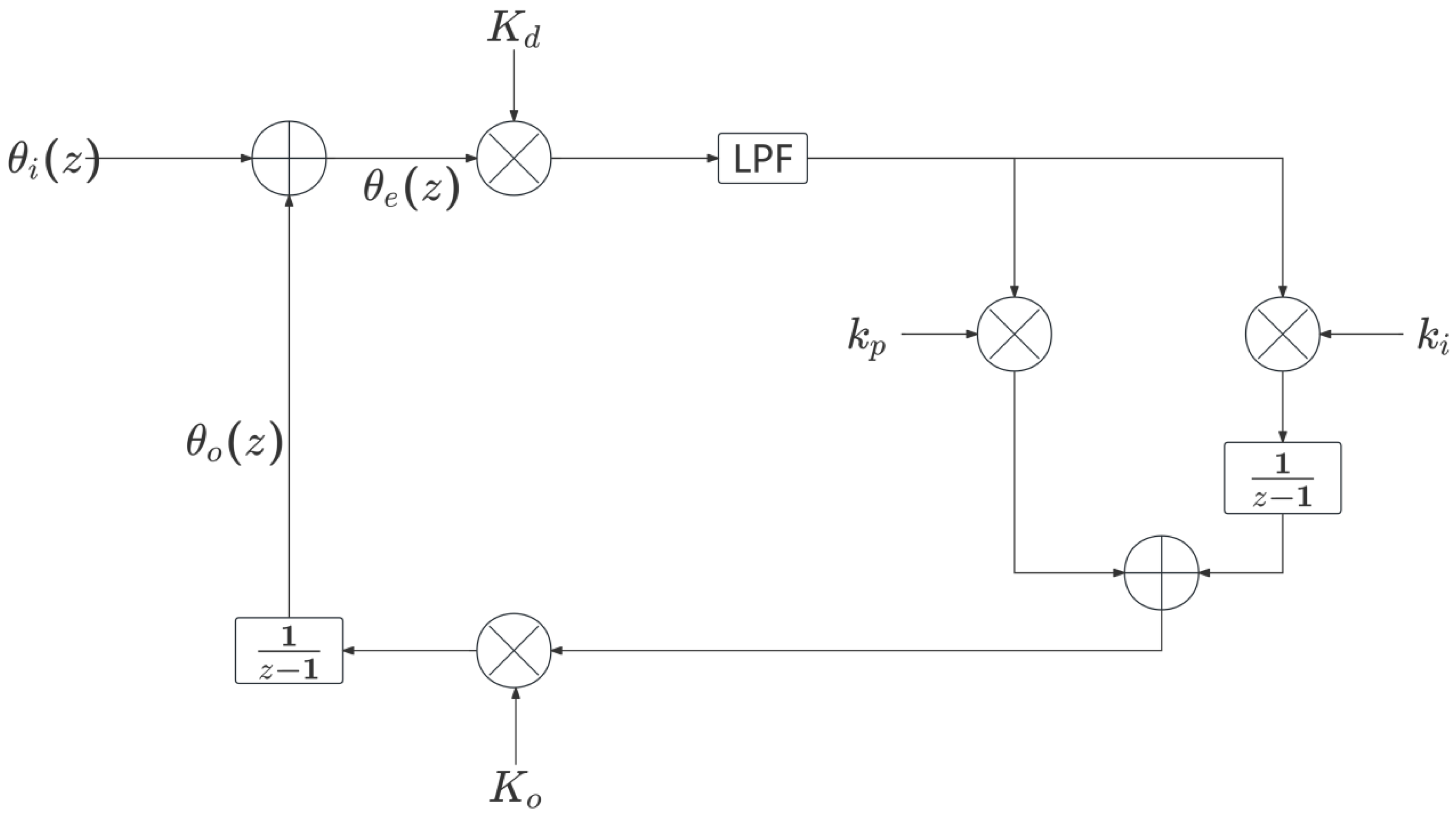
For frequency-domain analysis of the phasemeter system, consider its phase transfer function in Figure 5. Here, the phase detector acts as a subtractor for phases, the LPF filters the phase, serving as input to the PI controller to control the NCO’s frequency control word; ultimately, the NCO outputs a value close to the input phase for phase detection.

3.2.1. Digital Phase Detector (DPD)

There are three logical implementations for digital phase detectors: the XOR gate phase detector, the frequency-phase detector, and the edge-triggered phase detector. It is simply represented here as a multiplier. Its role is to multiply the in-phase and quadrature signals from the lookup table with the input signal to separate amplitude and phase information. The digital phase detector gain does not consider the LPF, so the gain value depends on the multiplier’s multiplication coefficient and the effective bandwidth of input and feedback signals, i.e., the amplitude of digital signals A / 2 .
F P D = 1 2 K m U i U 0
The phase detector gain is generally expressed as F P D , unit [V/rad], its value determined by the bit width of the two signals, generally a constant.

3.2.2. Low-Pass Filter (LPF)

The main role of the LPF in DPLL is to filter out high-frequency components in the quadrature signal, leaving low-frequency signals. Since the phasemeter is best modeled as a linear time-invariant system, a finite impulse response filter (FIR) is used for low-pass filtering before entering the PI controller. The LPF transfer function can be expressed as F L P F ( z ) :
F L P F ( z ) = n = 0 N 1 h ( n ) z n ,
where h ( n ) is the unit impulse response, with N taps. z n indicates signal delay by n sampling periods.

3.2.3. PI Controller

The PI controller used here is a first-order proportional–integral controller, its transfer function expressed as F P I ( z ) :
F P I ( z ) = k p + k i z 1

3.2.4. Numerically Controlled Oscillator (NCO)

The phasemeter’s NCO includes PIR, PA, and LUT. The increment register causes a delay z D , where D is the number of delayed clock cycles, determined by the number of registers. The phase accumulator can be simply expressed as a forward Euler accumulation process. The lookup table pre-stores discrete amplitude values of sine waveforms, directly indexed by phase value; the transfer function does not involve this nonlinear part, but the input to the NCO is the frequency control signal and the NCO’s frequency control sensitivity K o , unit [ rad / ( s · V ) ]:
K o = 2 π f c l k 2 B N C O ,
where f c l k is clock frequency and B N C O is phase accumulation word bit width. Therefore,
F N C O ( z ) = z D ( 1 z 1 ) 2 π f c l k 2 B N C O

3.2.5. Open-Loop Transfer Function

The open-loop transfer function of the phasemeter describes the transfer characteristics from the system input signal to a specific node (usually loop filter output or voltage-controlled oscillator input) in the open-loop state without feedback. In phase-locked loop systems, the open-loop transfer function is a key tool for analyzing and designing system performance. Generally, the open-loop transfer function can be calculated by breaking the phase-locked loop feedback path and considering the forward channel (including the phase detector, loop filter, and NCO, in part or in their entirety) transfer function. Considering the phasemeter needs appropriate bit width changes, C represents the bit width of the input and output changes in each link in the open-loop transfer function, and the gain caused by this shift is denoted as 2 C ; the open-loop transfer function is denoted G D P L L ( z ) :
G DPLL ( z ) = F PD F PLF F PI F NCO = 1 2 K m U i U 0 n = 0 N 1 h ( n ) z n k p + k i z 1 z D 1 z 1 2 π f clk 2 B NCO · 2 C

3.2.6. Closed-Loop Transfer Function

The closed-loop transfer function of the phasemeter describes the response characteristics of the phase-locked loop system to input signals. The closed-loop transfer function is usually expressed as H D P L L ( z ) :
H D P L L ( z ) = θ o u t ( z ) θ i n ( z ) = G D P L L ( z ) 1 + G D P L L ( z )

3.2.7. Error Transfer Function

The error transfer function of the phasemeter (DPLL) describes the error phase relationship between the input signal and the system output signal. The error transfer function is a key component in phase-locked loop analysis, helping understand how the phase-locked loop tracks input signal phase changes and reduces error. According to the feedback system equation, the error transfer function is usually expressed as:
E D P L L ( z ) = 1 H D P L L ( z ) = 1 1 + G D P L L ( z )

3.3. Steady-State Phase Error

The frequency ramp excitation signal occurring at zero time can be expressed as:
θ i ( n ) = 1 2 Δ ω ˙ n 2 u ( n ) ,
where Δ ω ˙ is the frequency ramp excitation amplitude and u ( n ) is the unit step sequence. So, its Z-transform can be expressed as:
θ i ( z ) = Δ ω ˙ z ( z + 1 ) 2 ( z 1 ) 3
Under such excitation, according to the previous error signal transfer function, considering the stable situation, the LPF transfer function approximates 1; ignoring the shift, the steady-state phase error final value of the error signal is:
lim n θ e ( n ) = lim z 1 ( z 1 ) E DPLL ( z ) θ i ( z ) = Δ ω ˙ k i F PD K o
Since the phasemeter system sampling rate is 100 MHz, the calculation error between continuous and discrete domains is small. The Laplace transform standard form for a second-order phase-locked loop is:
H ( s ) = K k p s + K k i s 2 + K k p s + K k i = 2 ξ ω n s + ω n 2 s 2 + 2 ξ ω n s + ω n 2 ,
where K is the loop gain, ω n is the natural angular frequency, and ξ is the damping coefficient. Obtain:
lim n θ e ( n ) = Δ ω ˙ ω n 2
When the bandwidth of the phasemeter is designed to be 100 kHz, which is the natural angular frequency, the maximum rate of change in Doppler frequency shift is approximately 100 Hz/s. Therefore, the steady-state phase error is:
lim n θ e ( n ) 1.59 × 10 9 rad 1 × 10 6 rad
Theoretical analysis shows that the steady-state phase error meets the requirement of 1 μ rad / Hz . However, in practical situations, experimental results often require consideration of multiple factors, which are far more complex than theoretical analysis. Therefore, in the following sections, this article will verify the correctness of the theory through experiments.

4. Hardware Experiments and Analysis

4.1. Experimental System Design

This paper mainly uses an FPGA (Field-Programmable Gate Array) for circuit design and experiments. FPGA is a semi-custom integrated circuit that can define its internal logic functions through hardware description languages (Verilog) or graphical tools, enabling flexible configuration from simple combinational logic to complex system-on-chip. Unlike ASIC’s “one-time customization,” FPGA logic functions can be erased and reconfigured multiple times after the factory, combining hardware high performance and software programmability, a core device for “rapid prototyping verification” and “small-batch applications” in digital system design.
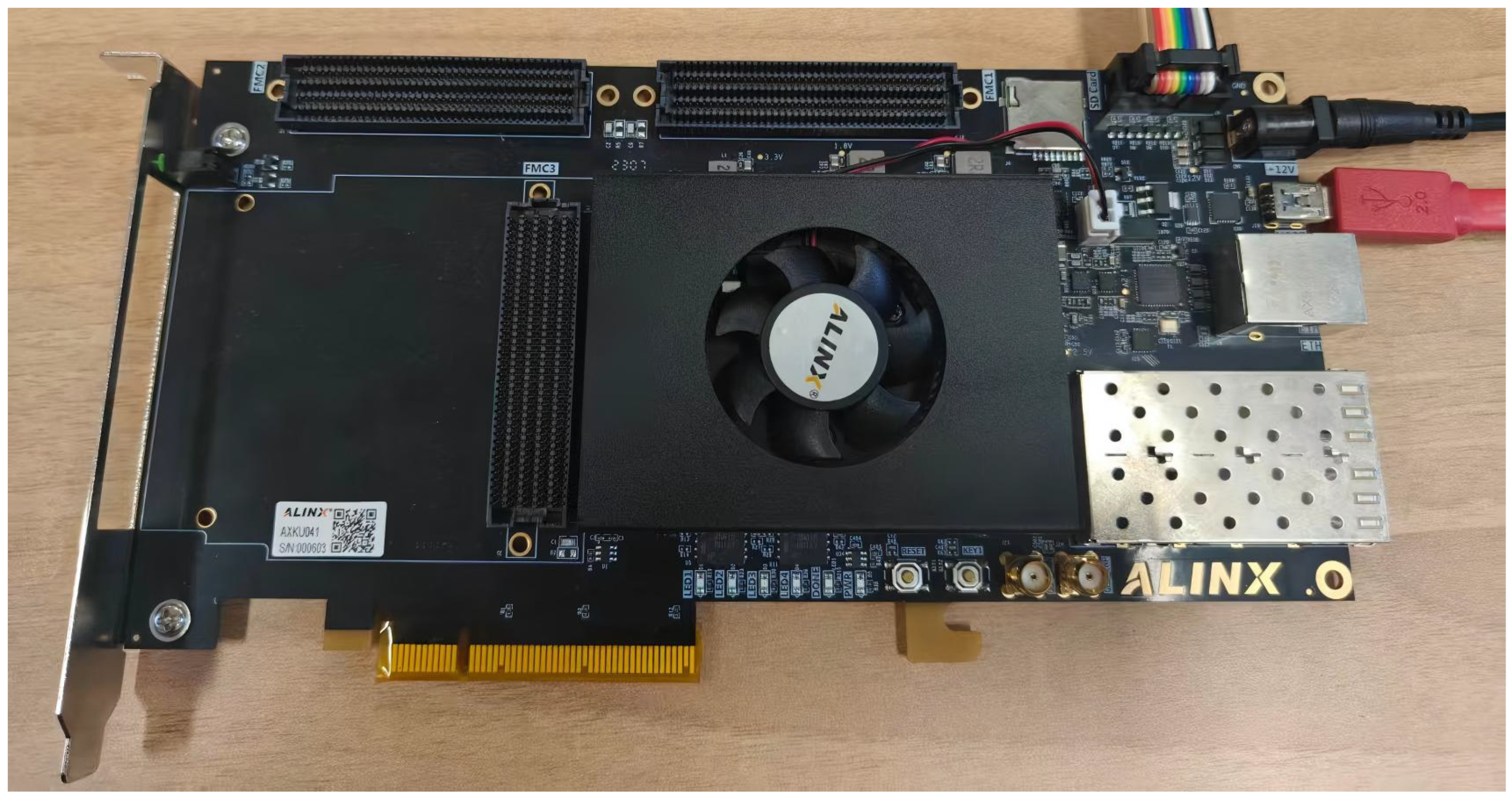
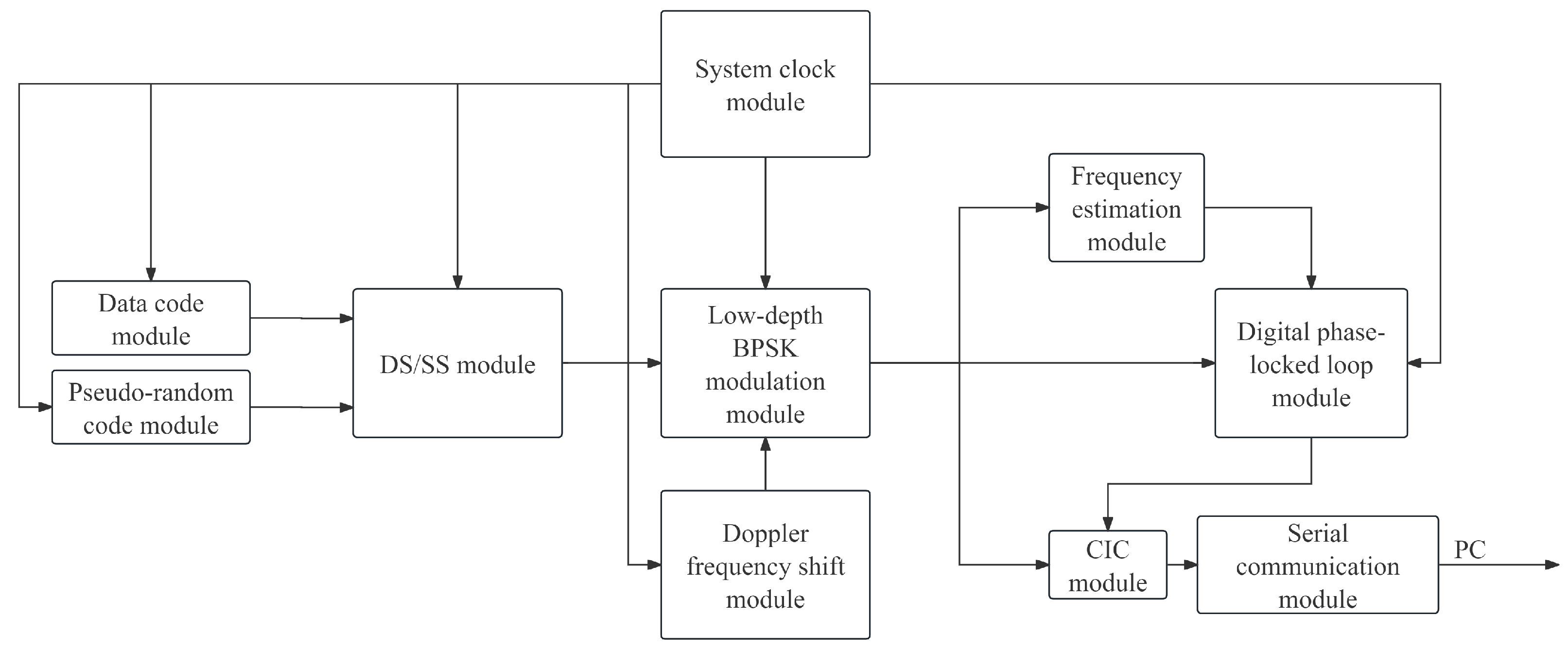
The FPGA chip in Figure 6 is an xcku040-ffva1156-2-i. The hardware is programmed through Vivado 2023.2 software. It has a designed system clock module, data code module, pseudorandom code module, DS/SS module, low-depth BPSK modulation module, phasemeter module, CIC module, and serial communication module. Finally, the serial communication module is used for post-processing the input data. The schematic diagram of the FPGA experiment is shown in Figure 7.
The system clock module mainly generates a 100 MHz single-ended clock from a 200 MHz differential clock, used as a 100 MHz sampling rate. To maintain synchronous clock domains, the system clock module is uniformly connected to each module as a clock signal.
The data code module and the pseudorandom code module mainly generate data codes and pseudorandom codes as data transmission carriers and perform XOR and spread spectrum in the DS/SS module to form communication ranging codes.
The Doppler shift module mainly simulates the generation of Doppler shift data between satellites, with a Doppler shift rate of 100 Hz/s, fed as an input to the low-depth BPSK modulation module as part of its carrier frequency.
The low-depth BPSK modulation module’s role is to modulate the input signal to the carrier frequency and carrier phase, where the Doppler shift is modulated to the carrier frequency through the frequency control word, and the communication ranging code is modulated to the carrier phase through the phase control word, and phase-modulated to bipolar code, i.e., communication ranging code 1 corresponds to 1, 0 to −1. Frequency control word and phase control word bit widths are both designed as 45-bit data.
The frequency control word sets a digital encoding value for the output signal frequency by controlling the phase accumulator step, which determines the phase change rate per unit time (i.e., frequency). The output signal frequency is determined by K, the system clock frequency is f c l k , and the accumulator bit number is N:
f o u t = K f c l k 2 N
To ensure signal frequency is within the hardware’s effective output range, the K range is 0 to 2 N 1 . The phase control word sets the digital encoding value for the output signal phase offset by adding a fixed offset to the base phase of the phase accumulator output, adjusting the signal’s initial phase or real-time phase. Basic formula for phase offset:
Δ ϕ = P 2 π 2 M ,
where P is the phase control word and M is the phase control word bit width. The phase offset unit is [rad].
The frequency estimation module mainly performs frequency estimation on the low-depth BPSK modulation module-simulated laser interferometry displacement signal, mainly using FFT on signal sampling points for frequency estimation. Since higher FFT frequency resolution consumes more hardware resources, the computation length used is 4096 and the frequency resolution is 24.41 kHz.
Simultaneously, the low-depth BPSK modulation module signal is input to the phasemeter module, which reads the input signal phase information and the error signal in the phasemeter.
As shown in Figure 4, the s i n signal output by the low-depth BPSK modulation module is directly used for phase detection with the c o s signal output by the NCO in the phasemeter module. It should be noted that the laser interferometric displacement measurement signal discussed earlier was a c o s signal. Here, in order to facilitate the removal of the negative sign in the Q-channel signal output for comparison with the original communication ranging code, the signal is changed to s i n for phase detection with the quadrature signal.
The signal after the phase detection through the LPF is output as a Q-path signal for subsequent delay-locked loop pseudocode ranging. The communication ranging code can be compared with the Q-path signal for consistency through a hardware experiment. The other path directly inputs the PI controller to control the NCO output frequency, where the PI controller output needs an additional initial frequency to avoid too large a difference with the input signal frequency, leading to the phasemeter being unable to lock. In FPGA, high-order cascaded integrator comb (CIC) filters are commonly used as anti-aliasing filters [23]. PA in NCO outputs an absolute phase and enters the CIC module for filtering the absolute phase, as shown in Figure 8. The CIC filter frequency is set to 10 Hz, fully retaining the gravitational wave band information.
Its transfer function and amplitude-frequency response are:
H 3 r d ( z ) = ( 1 z D 1 z ) 3 ,
H 3 r d ( e j ω ) = sin ( ω D / 2 ) sin ( ω / 2 ) 3
The CIC module output data enters the serial communication module using the UART protocol. The UART (Universal Asynchronous Receiver/Transmitter) is an asynchronous serial communication protocol that is widely used for short-distance data transmission between devices; it is key to realizing hardware logic serialization and parallelization conversion of data, and no clock signal synchronization is needed (asynchronous communication).

4.2. Communication Ranging Signal Verification

The error signal, i.e., Q-path output signal, outputs a communication ranging code for subsequent pseudocode ranging. Here, the low-depth BPSK modulation module has an initial frequency of 10 MHz. The Doppler shift is modulated to a carrier frequency. The Doppler shift rate is 100 Hz/s using a 0.1 rad modulation index to modulate the communication ranging code to the carrier phase, i.e.,
u i ( t ) = sin 2 π ( f 0 + f D ) t + 0.1 p r n ( t )
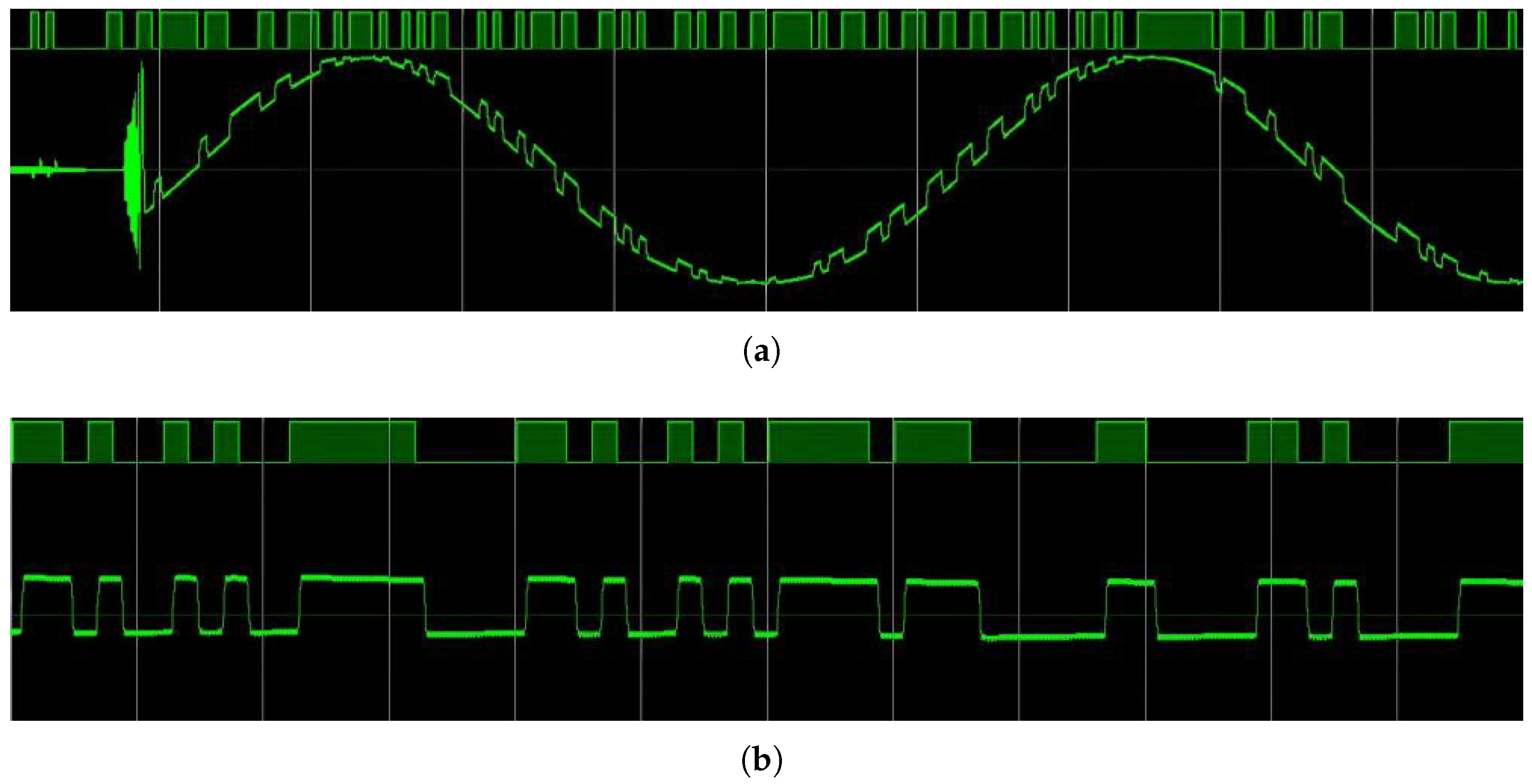
Here, no addition of ϕ d ( t ) from laser interferometry displaces the measurement model because the time integral of the Doppler shift is the displacement phase, and the experiment considers the initial displacement phase to be 0. Due to FFT and steady-state error limitations, we mainly discuss the impact of the kHz-level phasemeter bandwidth on the communication ranging signal. We input the low-depth BPSK modulation module’s output signal to the phasemeter module for communication ranging code demodulation, and obtain a Q-path signal time-domain diagram:
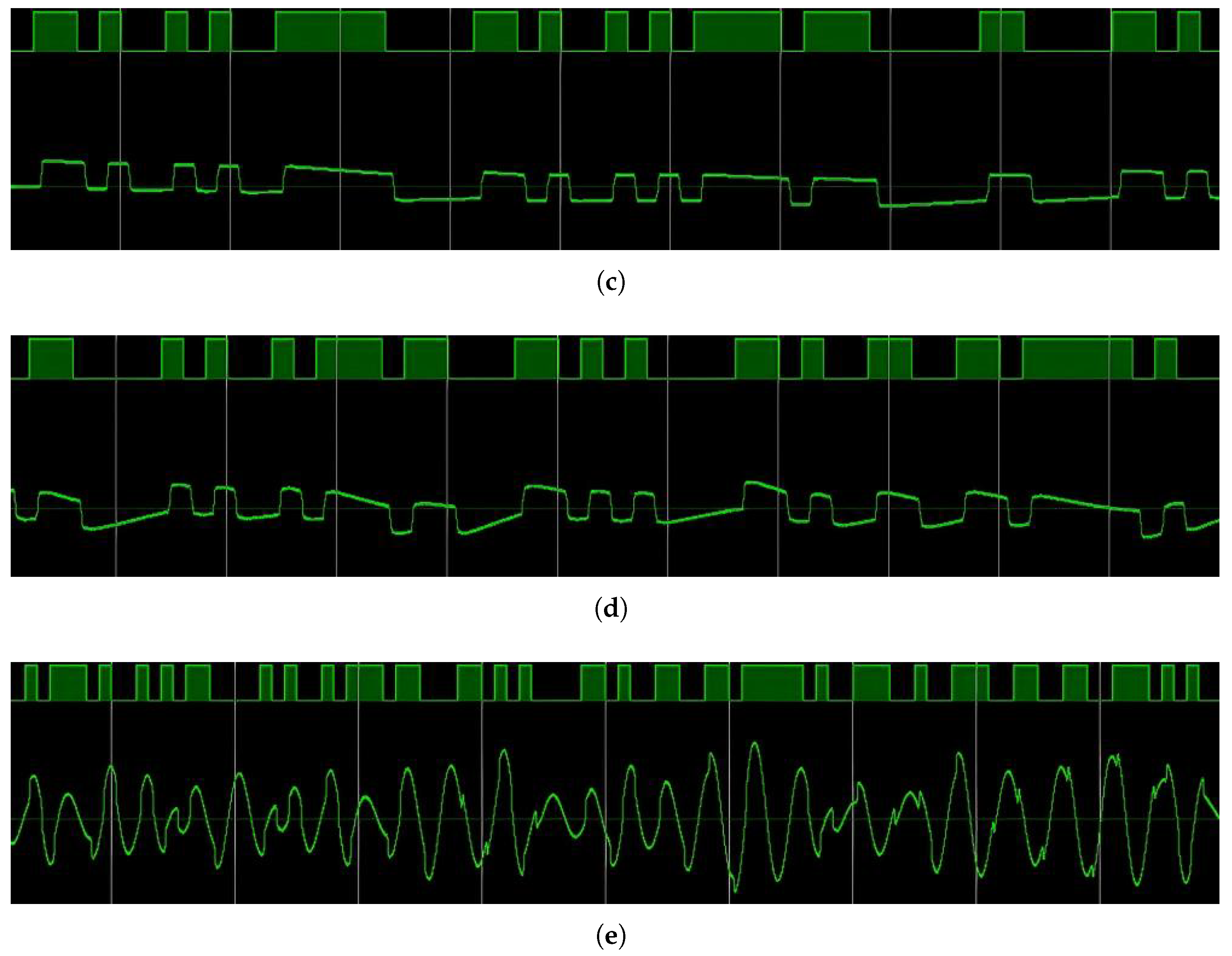
By comparing communication ranging signal time-domain diagrams under different bandwidths in Figure 9, under a 6.25 kHz bandwidth, the signal cannot lock quickly, and always has an oscillation interval. Such a communication ranging signal cannot satisfy subsequent DLL ranging. Under 1600 kHz bandwidth, too much noise enters, and the signal cannot correspond to the source code, making it unable to demodulate the communication ranging code.
For 25 kHz, 100 kHz, and 400 kHz phasemeter bandwidths, the LPF output Q-path signal is consistent with the communication ranging code source waveform. The output is positive when the source code is 1 and negative when it is 0. The LPF output is very close to 0, also indicating from the side that the phasemeter has a locked input signal and completed the demodulation of the communication ranging code.
So, below, we mainly discuss the phase noise performance of 25 kHz, 100 kHz, and 400 kHz phasemeter bandwidths.

4.3. Phasemeter Background Measurement

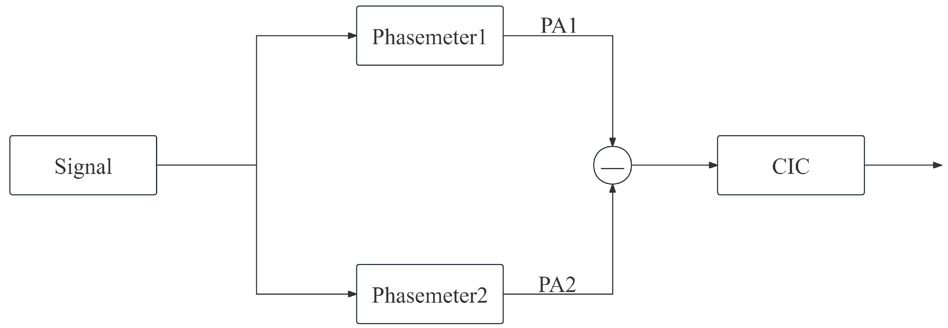
The phasemeter’s background noise, i.e., the phase noise, refers to the random phase fluctuations generated by the phasemeter itself at specific frequency offsets. In this paper, the phase noise amplitude spectral density units are [ rad / Hz ]. As can be seen in Figure 10, the phasemeter background noise is measured through differential phase measurements, separating the instrument’s own noise contribution.
The input signal is passed through two identically designed phasemeters in the NCO phase to measure the difference. Then, the signal is input to the CIC for decimation filtering. Finally, it is input to the serial module of the PC for data post-processing. Finally, we calculate its amplitude spectral density. The calculation formula as follows:
Δ θ ( t ) = S P A 1 ( t ) S P A 2 ( t ) 2
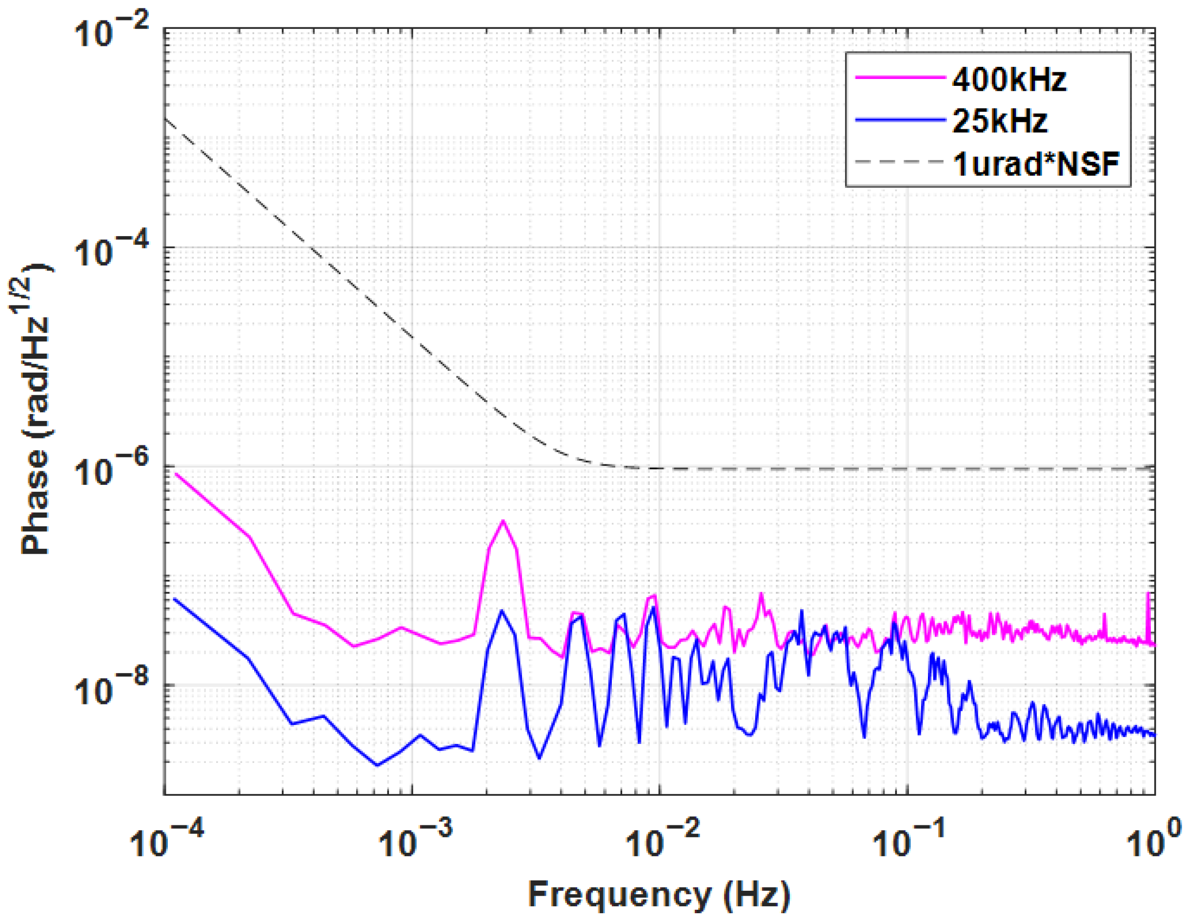
As can be seen in Figure 11, for phasemeter bandwidths 25 kHz and 400 kHz, phasemeter backgrounds both satisfy the 1 μ rad / Hz requirement. The 400 kHz phasemeter bandwidth is due to more white noise and spurious noise entering, so the phase noise curve is higher than 25 kHz bandwidth, but the system background noise also meets the phase noise requirements.

4.4. Influence of Doppler Shift on Phase Noise

First, consider the carrier signal without a Doppler shift, i.e., no Doppler shift added in the low-depth BPSK modulation module, which maintains the initial frequency of 10 MHz, i.e.,
u i ( t ) = sin 2 π f 0 t + 0.1 p r n ( t )
The signal is input to the phasemeter to extract the phase noise and obtain the phase noise result. Additionally, consider the Doppler shift data, i.e., the input signal:
u i ( t ) = sin 2 π ( f 0 + f D ) t + 0.1 p r n ( t )
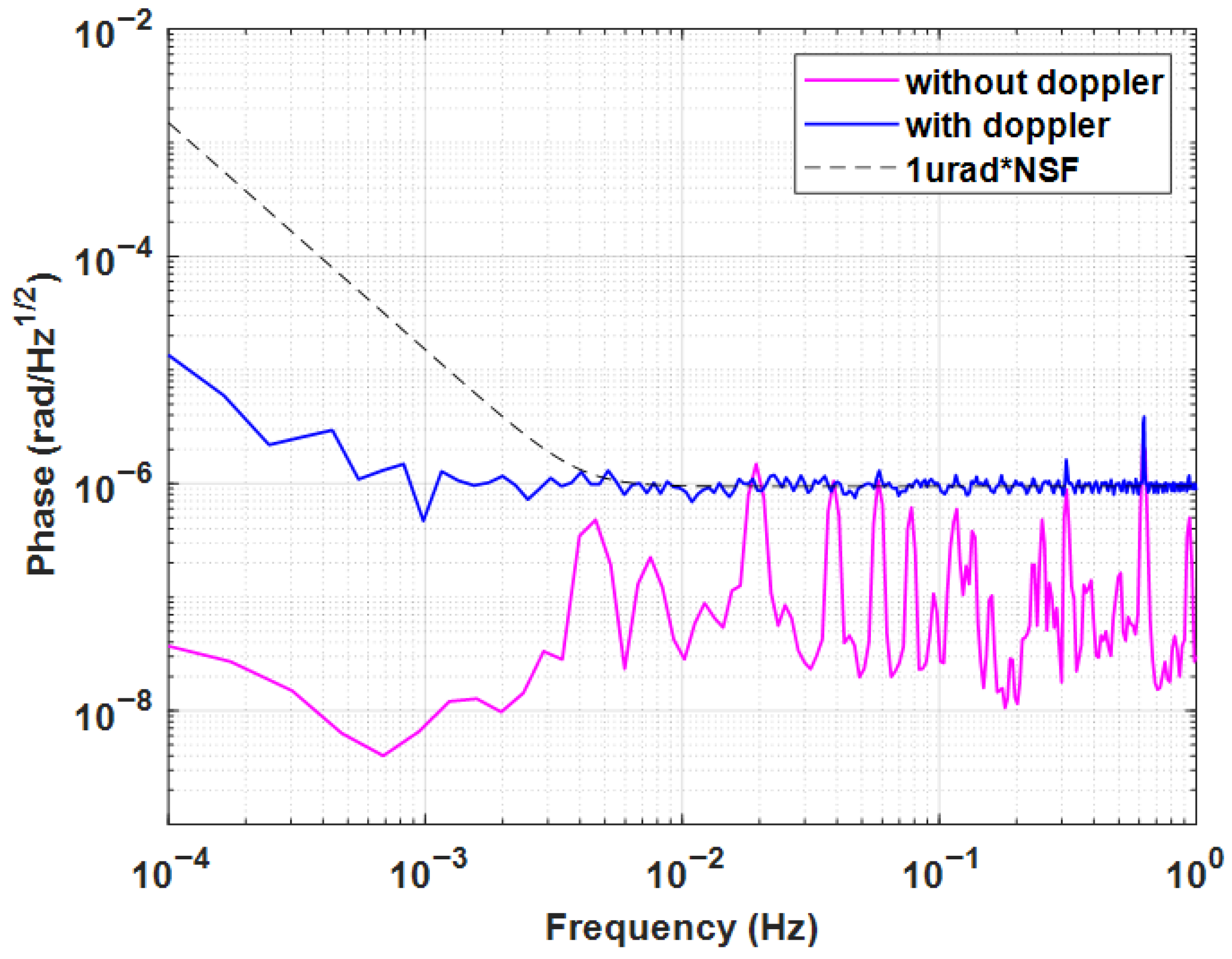
Obtain the phase noise with and without a Doppler shift under a 10 MHz carrier initial frequency, as shown in Figure 12.
The calculation formula is as follows:
Δ θ ( t ) = θ ( t ) S P A ( t )
As can be seen in Figure 13, the phase noise measurement method mainly measures the differences between the NCO output phase and the input signal phase, obtaining the amplitude spectral density. This phase noise reflects the phasemeter’s precise tracking and measurement ability for dynamic signals.
We compared phase noise curve diagrams after the phasemeter system for signals with and without varying Doppler shift under a 25 kHz bandwidth. As can be seen in Figure 13, a 100 Hz/s varying Doppler shift indeed elevates the phase noise curve due to the steady-state error, because under the 25 kHz bandwidth, the larger steady-state error makes the system unable to fully track the Doppler shift signal, and the pseudocode signal leads to an increase in phase noise.

4.5. Phase Noise Under Different Bandwidths

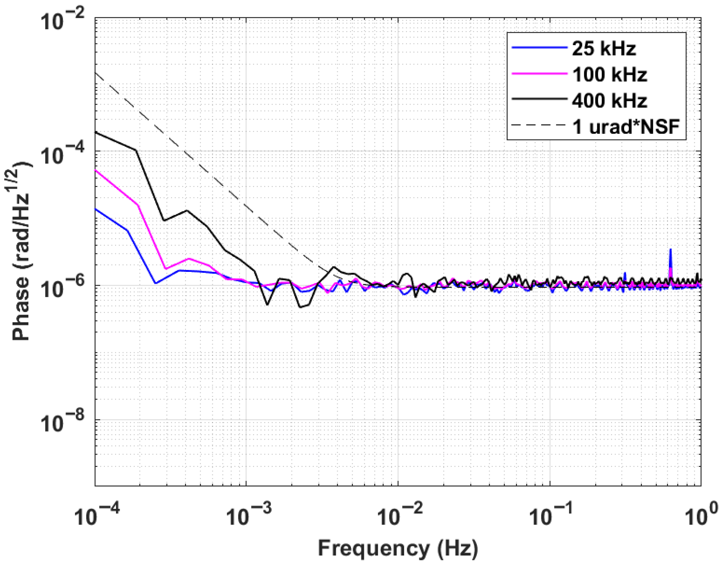
Here, we mainly discuss the phase noise performance of 25 kHz, 100 kHz, and 400 kHz phasemeter bandwidths. From Figure 14, a larger phasemeter bandwidth leads to a low-frequency band noise curve elevation, and the high-frequency band has no obvious difference. The 25 kHz bandwidth phase noise performs best, in which the system phase noise meets the 1 μ rad / Hz requirement.

5. Conclusions

The magnitude of steady-state phase error is mainly determined by two key factors: the rate of change in the Doppler shift and the operating bandwidth of the phasemeter. Specifically, when the rate of change in Doppler shift is low, its contribution to system phase noise is relatively weak, resulting in a low overall steady-state phase error. Meanwhile, the bandwidth setting of the phasemeter also significantly affects the distribution and magnitude of phase noise; a wider bandwidth makes the system more sensitive to rapid phase fluctuations, enhancing dynamic signal tracking capability but also introducing more noise.
Further analysis shows obvious differences in phase noise performance under different bandwidth conditions. When the phasemeter bandwidth is larger, in the low-frequency range, the phase noise curve exhibits a steeper rise; in contrast, in the high-frequency region, phase noise curves under different bandwidth settings show no significant differences, maintaining consistent change trends. This phenomenon indicates that bandwidth choice has a significant impact on low-frequency phase noise—a larger bandwidth leads to a higher low-frequency phase noise—while its influence on high-frequency phase noise is relatively limited.
The background phase noise performance of the designed phasemeter fully meets the system’s technical indicators. Bandwidth setting has a significant impact on communication ranging code signal performance: larger bandwidth improves the system’s tracking ability for dynamic signals, more effectively responding to rapidly changing signal features; however, increasing bandwidth also leads to a corresponding increase in low-frequency phase noise, negatively affecting system precision. On the other hand, varying Doppler shift directly affects the system’s steady-state phase error, and an increase in steady-state phase error further contributes to phase noise, forming a cumulative effect. Under typical operating conditions with a system bandwidth of 25 kHz and a Doppler shift rate of 100 Hz/s, comprehensive testing and verification demonstrate that the system’s phase noise level still strictly meets design requirements, demonstrating good stability and adaptability.
In summary, based on simulation and experimental data, considering the impact of bandwidth on tracking capability and steady-state error on phase noise, this article suggests using a phasemeter with a bandwidth of 25 kHz to 100 kHz in phase measurement.

Author Contributions

Conceptualization, Z.Y.; methodology, Z.X.; software, Z.X.; validation, Z.Y. and H.D.; formal analysis, Z.X.; investigation, Z.X.; resources, Z.Y.; data curation, Z.X.; writing—original draft preparation, Z.X.; writing—review and editing, Z.Y.; visualization, Z.X.; supervision, Z.Y.; project administration, Z.Y.; funding acquisition, K.L. All authors have read and agreed to the published version of the manuscript.

Funding

This research was funded by the National Key R&D Program of China (grant no. 2023YFC2205501) and Fundamental Research Funds for the Central Universities, Sun Yat-sen University.

Institutional Review Board Statement

Not applicable.

Informed Consent Statement

Not applicable.

Data Availability Statement

The original contributions presented in this study are included in the article; further inquiries can be directed to the corresponding author.

Conflicts of Interest

The authors declare no conflicts of interest.

Abbreviations

The following abbreviations are used in this manuscript:
ADCAnalog-to-Digital Converter
BPSKBinary Phase Shift Keying
CICCascaded Integrator Comb
DLLDelay-Locked Loop
DPLLDigital Phase Locked Loop
DS/SSDirect Sequence/Spread Spectrum
EOMElectro-Optic Modulator
FIRFinite Impulse Response
FPGAField-Programmable Gate Array
GWGravitational Wave
HPOPHigh-Precision Orbit Propagator
LIGOLaser Interferometer Gravitational Wave Observatory
LPFLow-Pass Filter
LUTLook-Up Table
NCONumerically Controlled Oscillator
PAPhase Accumulator
PIProportional–Integral
PMSPhase Measurement System
QPDQuadrant Photodetector
SCESignal Conditioning Electronics
STKSatellite Tool Kit
TDITime-Delay Interferometry
TMTest Mass
UARTUniversal Asynchronous Receiver/Transmitter
USOUltra-Stable Oscillator

Appendix A

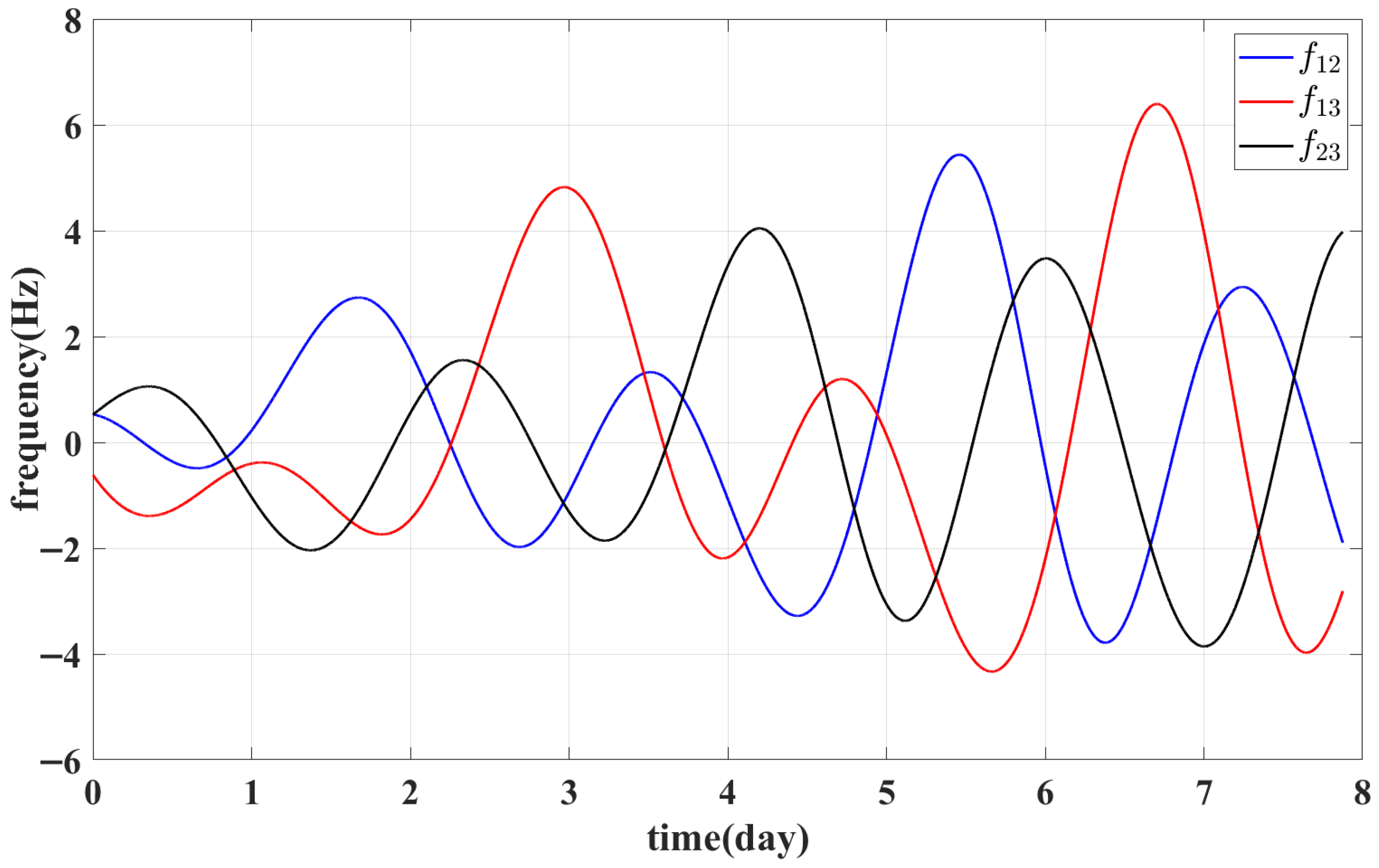
It should be noted that the orbital propagation was performed with a step size of 600 s. To verify that this granularity does not introduce significant errors in the Doppler shift estimation, we conducted a sensitivity test by reducing the step size to 1/60 of the original value. The simulation results are shown in Figure A1.
Figure A1. The 8-day simulation of Doppler shift between TianQin satellites. The step size is 10 s.
Technologies 14 00160 g0a1
It can be seen from the figure that there is no significant difference between the results with a step size of 10 s and 600 s. This is because the period of a satellite’s orbit around the Earth is a few days, so the Doppler frequency shift does not undergo a sudden change in just a few hundred seconds, and the rate of change in the Doppler frequency shift is the same.

References

  1. Einstein, A. Approximative integration of the field equations of gravitation. Sitzungsber. Preuss. Akad. Wiss. Berl. (Math. Phys.) 1916, 1916, 688–696. [Google Scholar]
  2. Sathyaprakash, B.S.; Schutz, B.F. Physics, astrophysics and cosmology with gravitational waves. Living Rev. Relativ. 2009, 12, 2. [Google Scholar] [CrossRef] [PubMed]
  3. Abbott, B.P.; Abbott, R.; Abbott, T.; Acernese, F.; Ackley, K.; Adams, C.; Adams, T.; Addesso, P.; Adhikari, R.X.; Adya, V.B.; et al. GW170814: A three-detector observation of gravitational waves from a binary black hole coalescence. Phys. Rev. Lett. 2017, 119, 141101. [Google Scholar] [CrossRef] [PubMed]
  4. Mooley, K.; Nakar, E.; Hotokezaka, K.; Hallinan, G.; Corsi, A.; Frail, D.; Horesh, A.; Murphy, T.; Lenc, E.; Kaplan, D.; et al. A mildly relativistic wide-angle outflow in the neutron-star merger event GW170817. Nature 2018, 554, 207–210. [Google Scholar] [CrossRef] [PubMed]
  5. Liang, Z.C.; Hu, Y.M.; Jiang, Y.; Cheng, J.; Zhang, J.d.; Mei, J. Science with the TianQin Observatory: Preliminary results on stochastic gravitational-wave background. Phys. Rev. D 2022, 105, 022001. [Google Scholar] [CrossRef]
  6. Abbott, R.; Abbott, T.D.; Abraham, S.; Acernese, F.; Ackley, K.; Adams, A.; Adams, C.; Adhikari, R.; Adya, V.; Affeldt, C.; et al. Observation of gravitational waves from two neutron star–black hole coalescences. Astrophys. J. Lett. 2021, 915, L5. [Google Scholar] [CrossRef]
  7. Luo, J.; Chen, L.S.; Duan, H.Z.; Gong, Y.G.; Hu, S.; Ji, J.; Liu, Q.; Mei, J.; Milyukov, V.; Sazhin, M.; et al. TianQin: A space-borne gravitational wave detector. Class. Quantum Gravity 2016, 33, 035010. [Google Scholar] [CrossRef]
  8. Ye, B.; Zhang, X.; Ding, Y.; Meng, Y. Eclipse avoidance in TianQin orbit selection. Phys. Rev. D 2021, 103, 042007. [Google Scholar] [CrossRef]
  9. Luo, J.; Bai, S.; Bai, Y.; Cai, L.; Dang, H.; Dong, Q.; Duan, H.Z.; Du, Y.; Fan, L.; Fu, X.; et al. Progress of the TianQin project. Class. Quantum Gravity 2025, 42, 173001. [Google Scholar] [CrossRef]
  10. Chen, Z.; Li, Z. Robust precise time difference estimation based on digital zero-crossing detection algorithm. IEEE Trans. Instrum. Meas. 2016, 65, 1739–1748. [Google Scholar] [CrossRef]
  11. Liang, Y.R.; Duan, H.Z.; Yeh, H.C.; Luo, J. Fundamental limits on the digital phase measurement method based on cross-correlation analysis. Rev. Sci. Instrum. 2012, 83, 095110. [Google Scholar] [CrossRef]
  12. Heinzel, G.; Wand, V.; Garcia, A.; Jennrich, O.; Braxmaier, C.; Robertson, D.; Middleton, K.; Hoyland, D.; Rüdiger, A.; Schilling, R.; et al. The LTP interferometer and phasemeter. Class. Quantum Gravity 2004, 21, S581. [Google Scholar] [CrossRef][Green Version]
  13. Ware, B.; Folkner, W.; Shaddock, D.; Spero, R.; Halverson, P.; Harris, I.; Rogstad, T. Phase measurement system for inter-spacecraft laser metrology. In Proceedings of the Sixth Annual NASA Earth Science Technology Conference, College Park, MD, USA, 27–29 June 2006. [Google Scholar]
  14. Gerberding, O.; Sheard, B.; Bykov, I.; Kullmann, J.; Delgado, J.J.E.; Danzmann, K.; Heinzel, G. Phasemeter core for intersatellite laser heterodyne interferometry: Modelling, simulations and experiments. Class. Quantum Gravity 2013, 30, 235029. [Google Scholar] [CrossRef]
  15. Schwarze, T.S.; Fernández Barranco, G.; Penkert, D.; Kaufer, M.; Gerberding, O.; Heinzel, G. Picometer-stable hexagonal optical bench to verify LISA phase extraction linearity and precision. Phys. Rev. Lett. 2019, 122, 081104. [Google Scholar] [CrossRef] [PubMed]
  16. Abich, K.; Abramovici, A.; Amparan, B.; Baatzsch, A.; Okihiro, B.B.; Barr, D.C.; Bize, M.P.; Bogan, C.; Braxmaier, C.; Burke, M.J.; et al. In-orbit performance of the GRACE follow-on laser ranging interferometer. Phys. Rev. Lett. 2019, 123, 031101. [Google Scholar] [CrossRef]
  17. Zhang, X.; Luo, C.; Jiao, L.; Ye, B.; Yuan, H.; Cai, L.; Gu, D.; Mei, J.; Luo, J. Effect of Earth-Moon’s gravity on TianQin’s range acceleration noise. Phys. Rev. D 2021, 103, 062001. [Google Scholar] [CrossRef]
  18. Bayle, J.B.; Bonga, B.; Caprini, C.; Doneva, D.; Muratore, M.; Petiteau, A.; Rossi, E.; Shao, L. Overview and progress on the Laser Interferometer Space Antenna mission. Nat. Astron. 2022, 6, 1334–1338. [Google Scholar] [CrossRef]
  19. Esteban Delgado, J.J. Laser Ranging and Data Communication for the Laser Interferometer Space Antenna. Ph.D. Thesis, Universidad de Granada, Granada, Spain, 2012. [Google Scholar]
  20. Zheng, L.; Yang, S.; Zhang, X. Doppler effect in TianQin time-delay interferometry. Phys. Rev. D 2023, 108, 022001. [Google Scholar] [CrossRef]
  21. Huang, X.; Wang, G.; Yang, M.; Yang, Z.; Cai, C.; Ming, M.; Zhang, J.; Yang, S.; Tu, L.; Duan, H.; et al. Study on picometer-level laser interferometer readout system in TianQin project. Opt. Laser Technol. 2023, 161, 109185. [Google Scholar] [CrossRef]
  22. Du, M.; Wang, P.; Luo, Z.; Han, W.B.; Zhang, X.; Chen, X.; Cao, Z.; Fan, X.; Wang, H.; Peng, X.; et al. Towards Realistic Detection Pipelines of Taiji: New Challenges in Data Analysis and High-Fidelity Simulations of Space-Borne Gravitational Wave Antenna. arXiv 2025, arXiv:2505.16500. [Google Scholar] [CrossRef]
  23. Yang, R.; Liu, H.; Luo, Z. Optimization Design of Decimation Filter for the Phasemeter in the Space Gravitational Wave Detection. IEEE Trans. Instrum. Meas. 2024, 73, 7006508. [Google Scholar] [CrossRef]
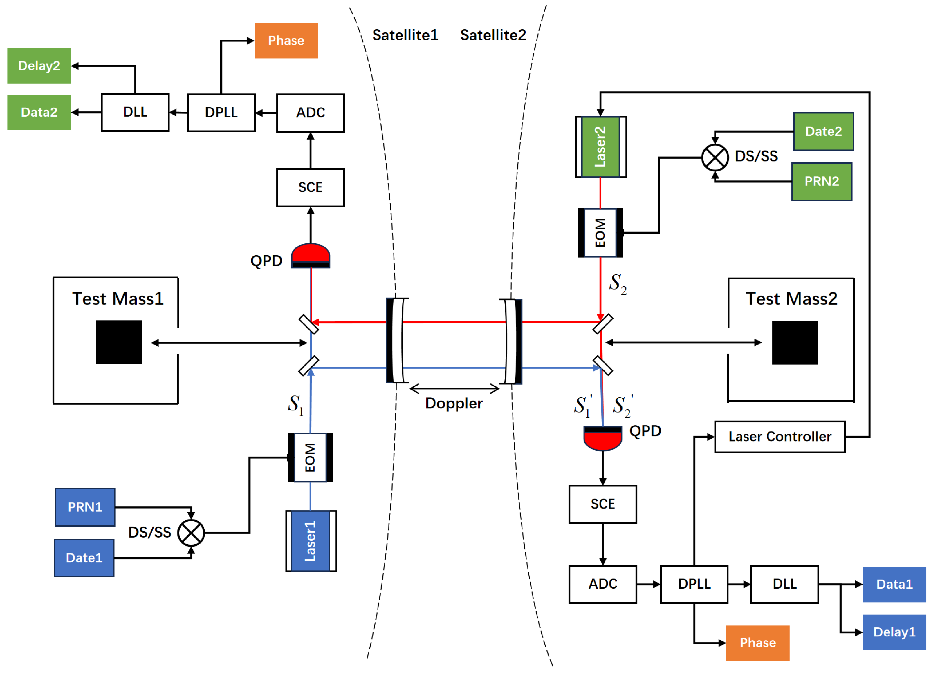
Figure 1. Schematic of inter-satellite laser interferometry system for gravitational wave detection, including laser sources, modulators, telescopes, detectors, and phasemeter modules.
Technologies 14 00160 g001
Figure 2. The 90-day simulation of Doppler shift between TianQin satellites, reaching ±8 MHz peak. Round-trip double Doppler shift approximately ranges from −6 to 8 MHz. Units: MHz.
Technologies 14 00160 g002
Figure 3. The 90-day simulation of Doppler shift rate of change, peaking at ±100 Hz/s, directly affecting phasemeter tracking performance. Units: Hz/s.
Technologies 14 00160 g003
Figure 4. Block diagram of a digital phasemeter for space gravitational wave detection, including a phase detector, PI controller, and NCO for phase tracking.
Technologies 14 00160 g004
Figure 5. Phase transfer function model of the phasemeter system, analyzing stability and tracking performance with key modules: detector, filter, PI controller, and NCO.
Technologies 14 00160 g005
Figure 6. Photo of AXKU041 development board (Xilinx Kintex UltraScale) used for phasemeter hardware implementation and Doppler simulation experiments.
Technologies 14 00160 g006
Figure 7. Block diagram of the FPGA-based experimental system for phasemeter performance verification, including clock, data generation, Doppler simulation, modulation, and communication modules.
Technologies 14 00160 g007
Figure 8. Structure of CIC filter for phase data decimation, reducing sampling rate from 100 MHz to 10 Hz while preserving gravitational wave frequency components.
Technologies 14 00160 g008
Figure 9. Time-domain communication ranging signals showing at different phasemeter bandwidths: (a) 6.25 kHz (unlocked); (b) 25 kHz (stable tracking); (c) 100 kHz (stable tracking); (d) 400 kHz (stable tracking); (e) 1600 kHz (excessive noise).
Technologies 14 00160 g009aTechnologies 14 00160 g009b
Figure 10. Schematic of differential phase measurement for phasemeter background noise isolation using two identical phasemeters.
Technologies 14 00160 g010
Figure 11. Phasemeter background noise at 25 kHz and 400 kHz bandwidths, both meeting requirements with slightly higher noise at 400 kHz. The NSF (Noise Shape Function) shown in the figures represents the allocated noise budget for the interferometric phase measurement in the TianQin mission. The “*” means a multiplication sign.
Technologies 14 00160 g011
Figure 12. Schematic of the phase noise measurement using the BPSK-modulated input signals.
Technologies 14 00160 g012
Figure 13. Phase noise comparison with/without 100 Hz/s Doppler shift at 25 kHz bandwidth. Doppler shift elevates low-frequency noise but remains within specifications. The “*” means a multiplication sign.
Technologies 14 00160 g013
Figure 14. Phase noise comparison at 25/100/400 kHz bandwidths. Larger bandwidth increases low-frequency noise, but all configurations meet the requirement. The “*” means a multiplication sign.
Technologies 14 00160 g014
Table 1. The initial elements of a set of optimized TianQin orbits in the J2000-based Earth-centered ecliptic coordinates at the epoch 22 May 2034 12:00:00 UTC [17].
Satellitea (km)ei (°)
SC1100,926.1584590.00030094.774822
SC2100,940.7890230.00001994.782183
SC3100,938.0564120.00041194.785623
SatelliteΩ (°)ω (°)ν (°)
SC1209.4330090.98087084.729131
SC2209.430454205.692143359.976125
SC3209.4382260.061831325.619846
Disclaimer/Publisher’s Note: The statements, opinions and data contained in all publications are solely those of the individual author(s) and contributor(s) and not of MDPI and/or the editor(s). MDPI and/or the editor(s) disclaim responsibility for any injury to people or property resulting from any ideas, methods, instructions or products referred to in the content.