Article

Enhancing Safe Exploration Through Subgoal Guidance

1
Moscow Independent Research Institute of Artificial Intelligence, Moscow 141701, Russia
2
Cognitive AI Systems Lab, Moscow 117312, Russia
*
Author to whom correspondence should be addressed.
Technologies 2026, 14(3), 146; https://doi.org/10.3390/technologies14030146
Submission received: 22 January 2026 / Revised: 21 February 2026 / Accepted: 26 February 2026 / Published: 28 February 2026
(This article belongs to the Section Information and Communication Technologies)

Abstract

Reinforcement learning is a widely used approach for autonomous navigation, but it often struggles to reach distant, long-horizon goals under safety constraints. The primary reason for this suboptimal performance is that safety requirements significantly degrade exploration capabilities during training, limiting the agent’s ability to discover feasible long-horizon policies. To address this issue, we introduce SG-Safe, a novel learning-based method that decomposes complex navigation tasks into smaller sub-problems using intermediate goals while respecting cumulative safety constraints. Our approach employs two coupled policies: a subgoal policy that generates intermediate subgoals, and a safe policy that leverages these subgoals to guide exploration toward the final objective. This hierarchical structure improves exploration without compromising safety and remains effective even under partial observability. We evaluate our method on autonomous vehicle navigation in simulation and using the Safety Gym benchmark. The experimental results demonstrate a strong safety–performance trade-off under partial observability. On Safety Gym, SG-Safe achieves an average success rate of 0.87 with a collision rate of 0.03, improving over the best end-to-end learning-based safe RL baseline (SR 0.40, CR 0.05). On POLAMP, SG-Safe attains SR 0.90 with CR 0.03, while the best single-policy safe RL baseline reaches at most SR ≤ 0.36 under the same observation settings. Moreover, on POLAMP, SG-Safe also surpasses the planning-based Lyapunov-RRT baseline that has access to full environment information, achieving higher success (SR 0.90 vs. 0.34) and a lower collision rate (CR 0.03 vs. 0.51), while eliminating online planning at deployment (PT = 0 s vs. ≈10–30 s per episode).

1. Introduction

Deep Reinforcement Learning (RL) has shown significant success in autonomous navigation [1], but its real-world application remains challenged by the safe exploration problem—learning efficiently while avoiding hazardous behaviors during training [2,3].
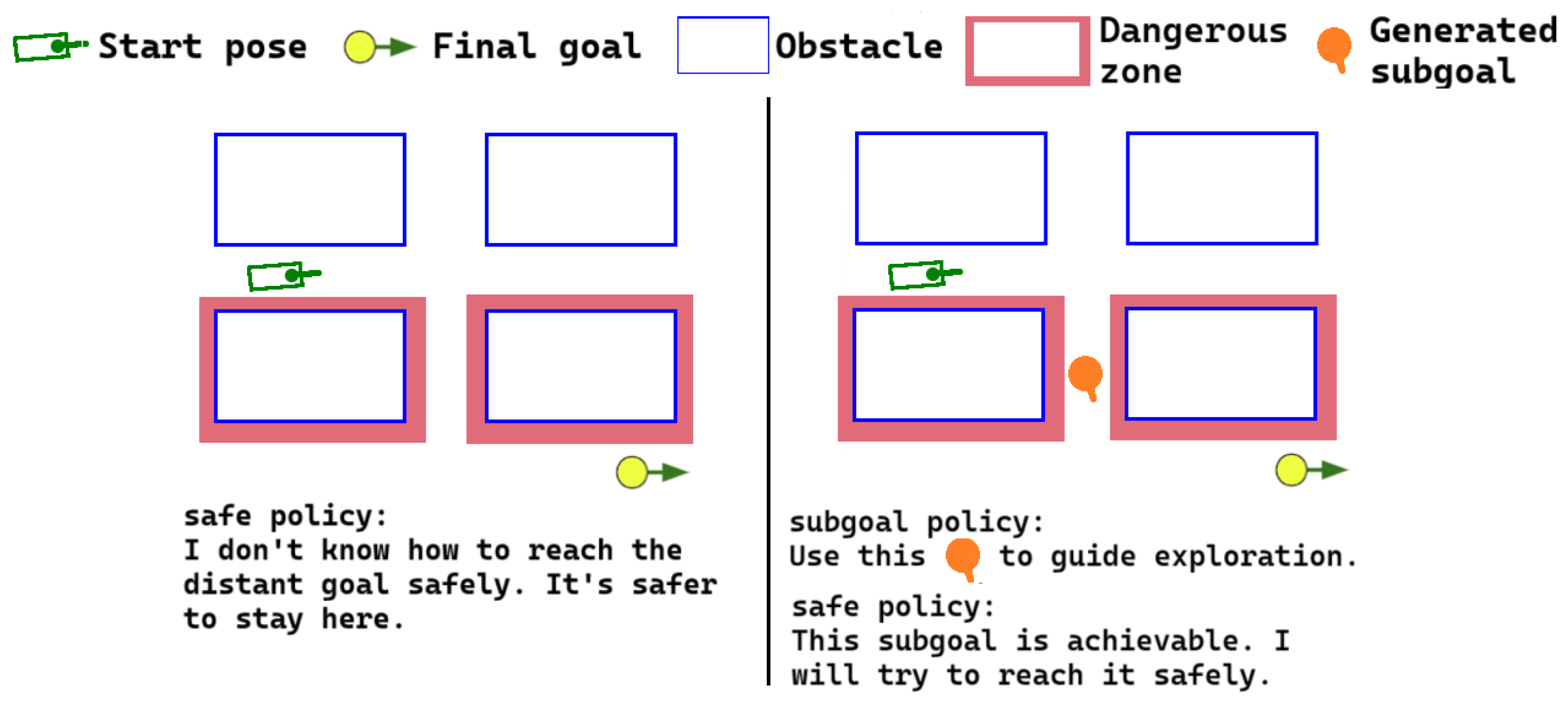
The Constrained Markov Decision Process (CMDP) is a standard framework for Safe RL, extending Markov decision processes with safety constraints [4]. While Lagrangian methods transform CMDPs into unconstrained problems via Lagrange multipliers [5], these approaches fundamentally limit exploration. Agents become overly conservative, avoiding potentially rewarding behaviors that might involve temporary constraint violations (Figure 1), creating a fundamental exploration–safety trade-off [6].
The problem intensifies in long-horizon navigation tasks that require extended sequences of actions, such as maneuvering around obstacles or navigating tight warehouse spaces. Solving such tasks requires extensive exploration, which inevitably leads to a high rate of safety constraint violations. Faced with this dilemma, conventional Safe RL agents often learn overly conservative behaviors, preferring to remain stationary rather than attempt to solve the task [7,8]. Thus, current Safe RL methods face two fundamental challenges: (1) the inability to solve long-horizon tasks due to insufficient exploration capabilities, and (2) the difficulty of adhering to safety constraints during the extensive exploration required for such tasks [9].
Few existing works attempt to combine Safe RL with Hierarchical Reinforcement Learning (HRL), a standard paradigm for solving long-horizon tasks due to its ability to facilitate extensive exploration through temporal abstraction. In contrast, other common techniques for tackling long horizons, such as curriculum learning or expert demonstrations, often demand significant engineering effort for reward shaping and scheduling or require additional human oversight. However, existing Safe HRL methods suffer from significant limitations: (1) they lack generalizability as they require additional environmental knowledge such as full observability or explicit cost function information; (2) they exhibit safety vulnerabilities at one of their hierarchical levels, either generating hazardous subgoals for the controller to pursue or employing a low-level controller unaware of safety constraints; and (3) they introduce substantial computational overhead during inference due to complex hierarchical planning mechanisms. For instance, Lyapunov RRT [10] combines an RRT* planner with a Lyapunov-based controller but requires full environment observability for planning, limiting its practical applicability. Moreover, its low-level controller operates solely based on robot kinematics, without incorporating any safety awareness, creating critical vulnerabilities during execution. Similarly, SafetyLayer + HiRO [9] integrates a learnable subgoal policy with a safety filter, but it suffers from generating subgoals in potentially dangerous regions that must be pursued by the controller. This approach also requires explicit cost function information and introduces computational overhead during subgoal generation, alongside complex optimization for action replacement. Other approaches [11,12,13] incorporate classical planners like A* with manually tuned safety penalties but intentionally avoid formal CMDP formulations. These methods consequently face significant reward engineering challenges and require extensive reward function tuning.
To address these gaps, we propose SG-Safe, a hierarchical CMDP method that enhances safe exploration through subgoal guidance. Unlike existing approaches, SG-Safe operates under partial observability without requiring explicit cost function knowledge. Our architecture employs dual policies during training: a subgoal policy for exploration guidance and a safe policy for constraint satisfaction. Crucially, during inference, only the safe policy is used, eliminating computational overhead while maintaining long-horizon task capability. This ensures efficient exploration during training, with safe, efficient deployment.
Our experimental results show that SG-Safe achieves a strong safety–performance trade-off among end-to-end learning-based Safe RL baselines under partial observability on the Safety Gym and POLAMP benchmarks. Additionally, on the POLAMP benchmark, SG-Safe outperforms planning-based baselines such as L-RRT and Lyapunov RRT that rely on privileged/full-state information, demonstrating strong performance in complex long-horizon corridor navigation under partial observability, while avoiding online planning overhead at deployment.
Our contribution is as follows:
  • We propose the integration of a subgoal policy to enhance the exploration ability of safe policies.
  • We show that the SG-Safe algorithm, operating under partial observability, outperforms the Lyapunov RRT algorithm (which relies on complete state information) in long-horizon tasks within the POLAMP environment [14], while achieving 10× faster inference.
  • We demonstrate that SG-Safe achieves strong results among end-to-end learning-based Safe RL baselines under partial observability on the Safety Gym and POLAMP benchmarks.

2. Related Work

2.1. Safe Reinforcement Learning

Safe RL addresses the challenge of maximizing rewards while adhering to safety constraints, typically framed as a CMDP [15,16]. Existing approaches fall into two main categories.
Optimization-based methods incorporate safety as an additional objective within the policy optimization process. Techniques such as Lagrangian methods [7] and constrained policy optimization [17] train critics to estimate cumulative cost, modifying the actor’s objective to balance reward and safety. While these approaches offer good generalization and require no explicit dynamics model, they lack strict safety guarantees during action execution. Despite their generality, constrained optimization methods (CMDP/Lagrangian) can be challenged by dual optimization instability and insufficient exploration, which become particularly severe in sparse-reward, long-horizon navigation tasks.
Control-theoretic methods employ safety filters to modify potentially unsafe actions. These include safety layers [18] that solve quadratic programming problems to find the nearest safe action, as well as control barrier functions (CBFs) [19] that provide formal safety guarantees through Lyapunov-like constraints. While offering stronger safety assurances, these methods typically require known dynamics models or cost functions and incur computational overhead from online optimization. Shielding methods [20,21] represent another approach that monitors and rejects unsafe actions, although they often remain limited to discrete action spaces.
Shielding and Black-Box Safe Exploration: A complementary line of work enforces safety via runtime intervention (shielding), where unsafe actions are filtered or corrected online. Many shielding approaches construct the shield from formal specifications such as linear temporal logic (LTL) or related logical formalisms, which typically require handcrafted rules, differentiable safety models, or privileged environment knowledge, limiting applicability in black-box settings. More recently, black-box post-shielding methods such as ADVICE [22] learn a safety discriminator from trajectories using contrastive representation learning and apply a non-parametric action filter during execution, without requiring a dynamics model or handcrafted safety rules, at the cost of additional inference-time filtering overhead.

2.2. Hierarchical Reinforcement Learning

Hierarchical Reinforcement Learning (HRL) addresses long-horizon tasks through temporal abstraction and task decomposition [23]. By introducing higher-level policies that set subgoals for lower-level controllers, HRL methods enhance exploration and mitigate credit assignment problems in complex environments.
Key challenges in HRL include non-stationarity from evolving lower-level policies and subgoal feasibility. Methods address these through off-policy corrections [24], adjacency-based subgoal generation [25], and lookahead planning [26]. Some approaches [9] employ a hierarchical structure exclusively during training to accelerate learning, while maintaining a flat policy during execution.

2.3. Hierarchical Safe Reinforcement Learning

The integration of hierarchical learning with safety constraints remains underexplored. Lyapunov RRT [10] combines RRT* planning with neural Lyapunov functions to generate safe trajectories, but it requires full environmental knowledge. Another approach integrates SafetyLayer with HIRO [9], using a differentiable cost function to generate intermediate subgoals that must be strictly achieved by the controller. This method suffers from computational overhead during inference due to per-action optimization and requires exact subgoal attainment.
In contrast, our approach differs in several key respects: (1) we operate under partial observability without requiring full state information; (2) our safety constraints are applied only during training rather than inference, eliminating inference-time optimization/shielding overhead; and (3) our safe policy dynamically balances exploration and safety constraints without requiring exact subgoal attainment. This approach maintains safety while reducing inference-time computational demands and improving exploration in long-horizon navigation tasks. This directly contrasts with prior Safe HRL methods that typically either rely on privileged/full-state information (e.g., planning-based HRL) or enforce safety at inference time via online shielding/filtering with explicit cost models. What is novel in SG-Safe is the combination of POMDP operation with training-time safety penalties and subgoal-guided learning, while inference uses only the learned safe low-level policy (Table 1).
Overall, prior safe decision-making methods can be grouped into (i) optimization-based CMDP methods that learn a policy with cost critics (typically without formal deployment guarantees), (ii) runtime filtering/shielding methods (CBF/safety layer/MPC) that can provide stronger guarantees but require models and incur online optimization, and (iii) planning-based approaches that rely on privileged state information. SG-Safe belongs to group (i) but addresses long-horizon exploration under partial observability by subgoal-guided training while discarding the hierarchy at inference.

3. Problem Statement

We are interested in RL algorithms for navigation problems that take safety constraints into account. To this end, we model our problem as a CMDP, where the agent is required to produce a sequence of actions that transitions it from the start state to the goal while avoiding obstacles and ensuring a specified level of safety.
Formally, a CMDP can be represented as a tuple ( S , A , P , R , C i ,   d i , γ ) , i ( 1 , , K ) where S is the state space, A is the action space, P is the state-transition model, R is the reward function, C i is the i-th constraint cost function, and γ is the discounting factor. Additionally, we consider a goal-conditioned setting of the CMDP with the goal space G S . During learning, at each time step, the agent, being in state s t S with a given goal g t G , takes action a t A and receives a reward r t = R ( s t , a t , s t + 1 , g t ) and costs c i = C i ( s t , a t , s t + 1 , g t ) . The goal is to learn a policy, i.e., the mapping from the states to the distributions of actions, π : S P ( A ) . The policy should maximize the expected return J ( π ) from the start state s t while satisfying the discounted cost with cost limit d i through the discounted costs C i ( π ) under policy π :
J ( π ) = E τ π [ t = 0 T γ t r t ( s t , a t , s t + 1 , g t ) ]
C i ( π ) = E τ π [ t = 0 T γ t c i ( s t , a t , s t + 1 , g t ) ]
where τ = ( s 0 , a 0 , s 1 , a 1 , ) denotes a trajectory. The objective of the CMDP for the policy π is to find
π * = arg max π Π J ( π ) , s . t . C i ( π ) d i , i

4. Method

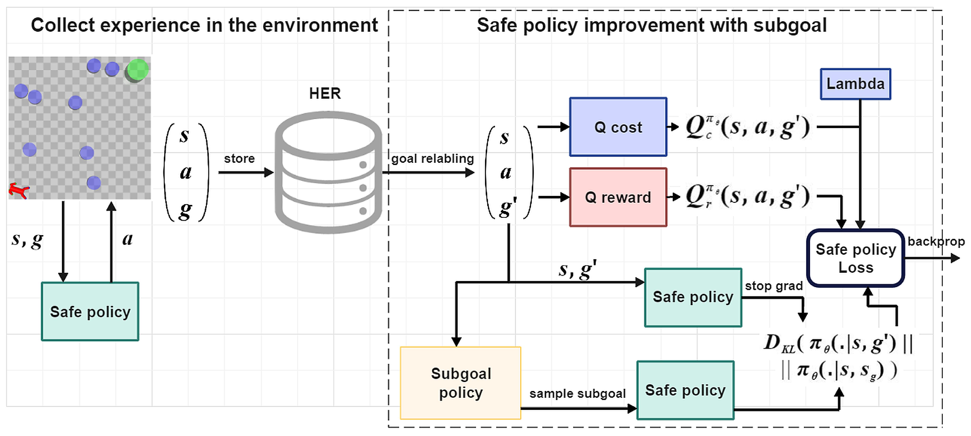
We propose SG-Safe, a method that combines a subgoal policy and a safe policy to solve constrained long-horizon tasks. The subgoal policy decomposes the task by proposing intermediate subgoals, improving exploration by guiding the low-level behavior toward feasible and informative states. The safe policy is trained under a Lagrangian objective to maximize task return while discouraging safety violations. As shown in Figure 2, SG-Safe alternates between two main procedures: (i) collecting experience with the safe policy and storing trajectories in a Hindsight Experience Replay (HER) buffer [27], and (ii) updating the safe policy using subgoals generated from replayed transitions to improve learning efficiency in sparse-reward, long-horizon settings.

4.1. Safe Policy

One of the most common approaches to addressing CMDPs is the Lagrangian method, often combined with the off-policy gradient algorithm SAC [28]. The Lagrangian method reduces the CMDP problem to an unconstrained optimization problem using Lagrange multipliers λ i (safety weights). These multipliers penalize constraint violations by measuring the discrepancy between the cost limit d i and the discounted expected cost C i ( π ) . Without loss of generality, we consider a single Lagrangian multiplier λ i = λ , cost limit d i = d , and discounted cost c = C i ( π ) = C ( π ) throughout this work. The soft Q-functions Q r π θ (reward) and Q c π θ (cost) are trained to minimize the soft Bellman residuals:
( Q r π θ ( s t , a t ) ( r t ( s t , a t ) + γ Q r π θ ( s t + 1 , a t + 1 ) α ent log π ( a t + 1 | s t + 1 ) ) ) 2
( Q c π θ ( s t , a t ) ( c ( s t , a t ) + γ Q c π θ ( s t + 1 , a t + 1 ) α ent log π ( a t + 1 | s t + 1 ) ) ) 2
where a t + 1 π ( a t + 1 | s t + 1 ) . The policy is optimized by minimizing the following Lagrangian objective:
L ( θ , λ ) = E α ent log π θ ( a t | s t ) Q r π θ ( s t , a t ) + λ Q c π θ ( s t , a t ) .
The Lagrange multiplier λ is learned adaptively by minimizing the following loss:
J s ( λ ) = E λ Q c π θ ( s t , a t ) d .
This update rule decreases the safety weight λ when the constraint is satisfied (i.e., Q c π θ ( s t , a t ) d ) and increases λ when the constraint is violated, thereby placing greater emphasis on safety.
We implement both reward and cost critics with twin Q-networks, i.e.,  { Q r , 1 , Q r , 2 } and { Q c , 1 , Q c , 2 } . For the Bellman targets, we use the minimum over the corresponding target critics to mitigate overestimation, and we maintain target networks for all critics updated by Polyak averaging with coefficient ( τ = 0.005). The next action a t + 1 is sampled from the current policy π θ , and the target value includes the standard SAC entropy term α ent log π θ ( a t + 1 s t + 1 ) . The entropy temperature α ent = 0.1 is treated as a fixed hyperparameter.

4.2. Subgoal Policy

The subgoal policy facilitates long-horizon task learning by generating intermediate subgoals between initial and goal states. Our approach builds on the RIS framework [8], which consists of two key components: a subgoal policy and a low-level policy. The imaged subgoal policy generates feasible subgoals that guide the low-level policy, while maintaining consistency with the agent’s state distribution through KL-divergence constraints.
The subgoal policy π H minimizes the maximum discounted steps to the subgoal or final goal, where V π θ represents the standard value function estimating the expected discounted reward. Specifically, ψ π θ ( s g | s , g ) = max ( | V π θ ( s , s g ) | , | V π θ ( s g , g ) | ) is minimized under a KL-constraint relative to the state distribution p s :
π H = arg max E [ A π k H ( s g | s , g ) ] , s . t . D KL ( π H ( · | s , g ) p s ( · ) ) ϵ
where the advantage function is defined as A π k H ( s g | s , g ) = E ψ π θ ( s | s , g ) ψ π θ ( s g | s , g ) , measuring the expected improvement in step reduction when updating the subgoal policy.
To train the low-level policy, a subgoal s g is sampled from π H for each transition. The low-level policy is then optimized to maximize the Q-value while minimizing the KL-divergence between the goal-conditioned and subgoal-conditioned action distributions:
π θ = arg max E Q r π θ ( s , a , g ) α D KL ( π θ ( · | s , g ) π θ ( · | s , s g ) ) .
This approach guides the low-level policy toward subgoals while maintaining alignment with the overall task objective.

4.3. Safe Policy with Subgoals

SG-Safe combines subgoal generation with constrained policy optimization to address safe exploration in long-horizon tasks. The safe policy autonomously balances task execution and exploration through adaptive subgoal guidance, dynamically adjusting its behavior based on environmental constraints and safety requirements. During training, subgoals guide exploration; during execution, only the trained safe policy is deployed.
The modified safe policy objective incorporates both task rewards and safety constraints:
J ( π θ ) = E ( s , g ) D E a π θ ( · | s , g ) [ Q r π θ ( s , a , g ) λ Q c π θ ( s , a , g ) α D K L π θ ( · | s , g ) π θ ( · | s , s g ) ] .
where Q r π θ maximizes the task reward, Q c π θ penalizes safety violations, and the KL-divergence term guides the policy toward generated subgoals, where D is the HER replay buffer.
The pseudocode of our approach is provided in Algorithm 1. Initially, experience is collected in the environment using only the safe policy ( π θ ( . | s , g ) ) and stored in a HER buffer. To improve convergence in sparse reward settings, we employ a HER buffer, which relabels failed episodes with achieved goals to provide more frequent learning signals. This approach significantly enhances sample efficiency and learning stability. Additional details about the relabeling strategy are provided in the Appendix E. Next, by sampling batches from the HER replay buffer, the reward and cost critics ( Q r π θ , Q c π θ ) are updated, along with both the safe policy and the subgoal policy ( π H ). Our experimental results demonstrated that, using an ensemble of two cost critics Q c π θ with min aggregation, selecting the minimum cost value between them provides the optimal balance between safety and performance. The subgoal policy generates the complete state vector as subgoal s g S , eliminating the need for manual goal space engineering required in other subgoal-based approaches [24,25,29]. This design choice justifies our adoption of RIS as the subgoal policy framework. Furthermore, the subgoals serve as regularization for the safe policy, enabling it to adaptively balance between environment exploration and safety maintenance.
Algorithm 1 SG-Safe
  1:
Initialize HER replay buffer D
  2:
Initialize Q r π θ , Q c π θ , π θ , λ , π H
  3:
for  k = 1 , 2 ,  do
  4:
     Collect experience in D using π θ in the environment
  5:
     Sample batch ( s t , a t , r t , c t , s t + 1 , g ) D
  6:
     Sample batch of subgoal candidates s g D
  7:
     Update Q r π θ , Q c π θ using soft Bellman residuals (Policy Evaluation)
  8:
     Update λ using Equation (7) (Multiplier Optimization)
  9:
     Update π H using Equation (8) (Subgoal Policy Improvement)
10:
     Update π θ using Equation (10) (Safe Policy Improvement with Subgoals)
11:
end for
The safe policy is implemented using an adapted version of SAC-Lagrangian. This approach enables the use of arbitrary cost functions without requiring their explicit specification or prior knowledge of the robot model, distinguishing it from other Safe RL methods (control barrier function, shielding, safety layer-based) that often depend on explicit dynamics modeling [18,19,20,21].

5. Experiments

In this section, we address the following research questions (RQs) through comprehensive experiments:
RQ1 (Safe Exploration Improvement): Does subgoal policy utilization in SG-Safe improve the safe exploration and task performance of the safe policy?
RQ2 (Comparison with Prior-Dependent Baselines): How does SG-Safe perform against methods requiring full environment observability or additional domain knowledge (e.g., Lyapunov-RRT), particularly in terms of task performance and inference-time efficiency?
RQ3 (Comparison with Baselines): How does SG-Safe compare against state-of-the-art Safe RL methods in terms of safety–performance trade-off?
RQ4 (Component Analysis): How do key hyperparameters (number of safety critics, algorithm parameters) affect the safety–performance trade-off in SG-Safe?
The experiments were conducted on the NVIDIA TITAN RTX. The average training time for the Safety Gym benchmark was 25 h, while for the POLAMP benchmark it was 48 h.

5.1. Environments

We evaluate our method on a series of challenging simulated navigation tasks designed to test long-horizon planning and safety constraint adherence under partial observability. Our primary benchmarks are based on the Safety Gym benchmark [6], extended with custom maps and task configurations to increase difficulty and facilitate a clearer analysis of safety–performance trade-offs. Additionally, we introduce the POLAMP [14] benchmark, featuring a kinematic agent navigating through narrow, cluttered corridors with precise turn constraints, presenting a more complex and realistic challenge for safe navigation algorithms.

5.1.1. Safety Gym Benchmark

Safety Gym is a standard testbed for Safe RL [6]. We employ its core robotic agents: the Point (differential drive), Car (Ackermann steering), Doggo (quadruped), and Sweeps (holonomic) platforms. Each agent receives proprioceptive state information (joint positions, velocities) and exteroceptive lidar-like observations detecting proximity to static hazards and goal locations. The observation space is goal-conditioned, concatenating the current agent state with the target goal vector. The task was considered to be solved if the agent reached the goal state with the Euclidean error ϵ ρ 0.3 m with no collisions. The reward is based on the Euclidean distance to the goal, and a cost (MTSC) of 1 is incurred for entering a hazardous zone.

5.1.2. POLAMP Benchmark

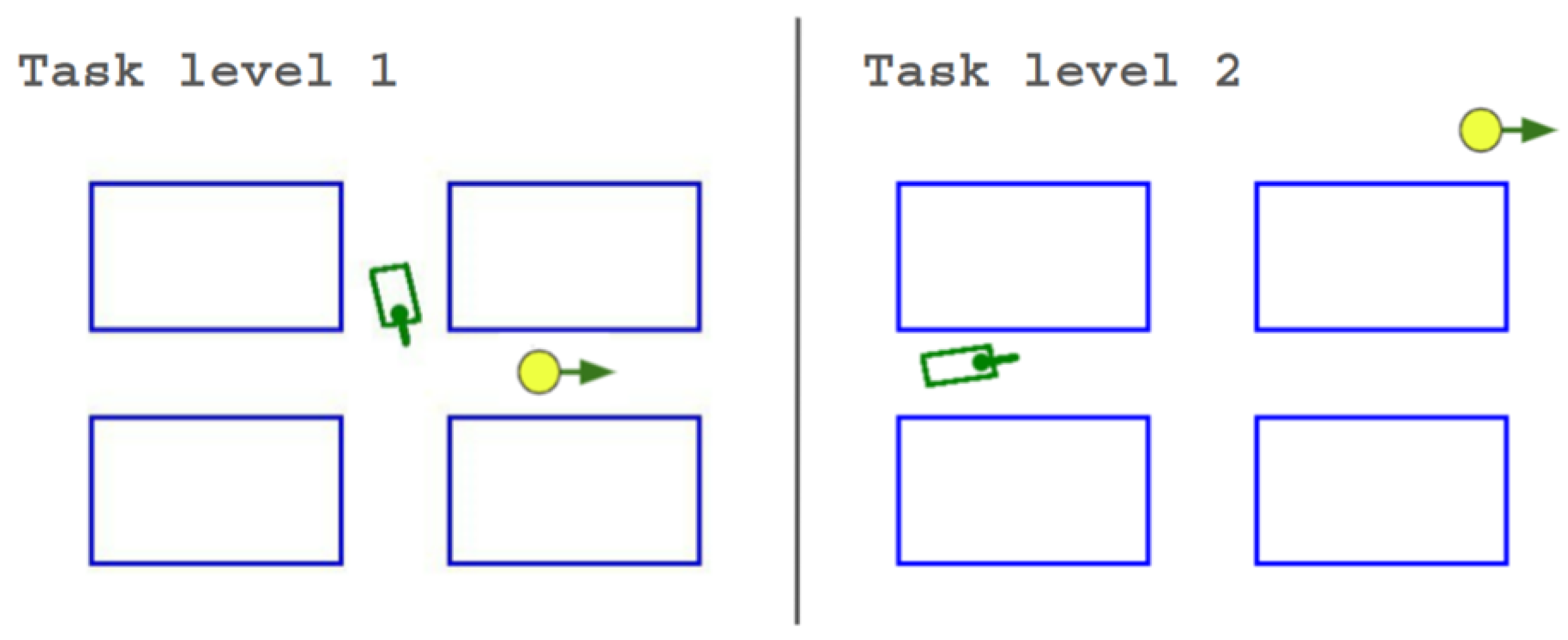
The POLAMP benchmark [14] features an autonomous vehicle with a kinematic bicycle model navigating environments with static obstacles (Figure 1). The agent is controlled through continuous linear acceleration and rotational velocity actions ( a t , ω t ) . Its observation space combines a 39-beam lidar scan (360° coverage, max range 10 m) with the robot’s internal state ( x , y , θ , v , γ ) . We assume a deterministic simulation without actuation noise. The reward is shaped by the Euclidean distance to the goal, while a cost (MTSC) is assigned for approaching any wall closer than 0.3 m. The benchmark includes two custom-developed datasets of increasing complexity: Level 1 and Level 2. Both datasets comprise 96 unique tasks. Additional dataset details and visualizations are provided in the Appendix B.

5.2. Evaluation Metrics

We evaluate all methods using three key metrics:
Success Rate (SR): The fraction of episodes successfully completed (higher is better).
Collision Rate (CR): The fraction of episodes terminated due to a collision with hazardous zones or obstacles (lower is better).
Mean Time Safe Cost (MTSC, t): C ( π ) , the average number of time steps the agent remains in proximity to hazardous zones or obstacles (lower is better).
These metrics collectively capture the trade-off between task performance and safety considerations, enabling comprehensive comparison across different approaches.

5.3. Baselines

We evaluate SG-Safe against comprehensive baselines across both environments, using a consistent set of hyperparameters. The only exception is the encoder module, which is exclusively employed for the POLAMP environment due to its higher-dimensional state space.
Safety Gym Benchmark: SAC, SAC-LAG, CPO [30], and Lyapunov RRT (L-RRT) [10]. All methods represent end-to-end RL policies except for L-RRT, which combines RRT* planner [31] with Lyapunov neural policy and assumes full observability. We maintain identical learning configurations except for CPO, which uses dense rewards from [6] instead of sparse rewards. We used a fixed entropy coefficient of α ent = 0.1 for the SAC policy and safety constraint limit d = 3.0 with Lagrangian initialization λ 0 = 0.5 .
POLAMP Benchmark: SAC, SAC-RBCF [19], SAC-LAG, SAC-NCMP [32], ADVICE [22], L-RRT, and classical RRT with Dubins steering [33]. SAC-RBCF employs quadratic programming to compute safe actions, while SAC-NCMP implements chance-constrained MDP with risk-bound Δ = 0.3 , sampling N action noises from N ( 0 , 1 ) per step to estimate the constraint violation probability N v / N . L-RRT was co-trained in obstacle-free environments with full state observation ( x , y , θ , v , δ ) and evaluated using geometric RRT* [10] with the following parameters: N max = 18,000 iterations, s t e p search = 0.1 , and  s t e p max = 5 . Each of the 96 tasks across difficulty levels 1–2 was executed 5 times to ensure statistical significance. ADVICE is a post-shielding approach: it learns a contrastive latent model of transitions to separate safe vs. unsafe regions and then applies an online non-parametric filter to replace actions predicted to be unsafe.
All learning-based methods share identical training configurations across both benchmarks. Specifically, CPO—being the simplest constrained RL baseline with limited empirical robustness—is included only in the Safety Gym benchmark, where tasks are lower-dimensional and easier; in the higher-dimensional and more dynamic POLAMP tasks, CPO consistently fails to learn meaningful policies. For the POLAMP benchmark, we additionally include the shielding-based baseline SAC-RBCF, which relies on access to robot dynamics for online quadratic-program safety filtering. This allows us to compare our method against the family of safety-filtering approaches that require privileged information unavailable to standard RL agents.

5.4. RQ1: Safe Exploration Improvement

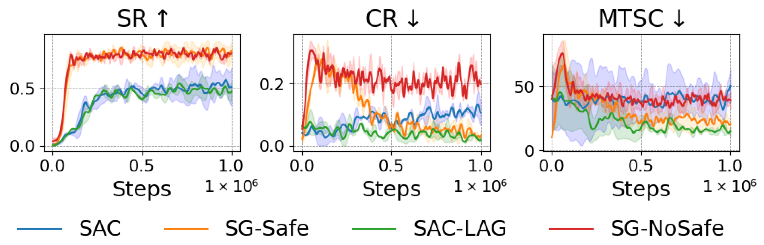
We conducted several experiments to evaluate how subgoal generation influences safe policy performance. We compared SG-Safe against three baselines: SAC, SAC-Lagrangian (SAC-LAG), and SG-NoSafe (see Figure 3). SG-NoSafe represents the original RIS method without safety constraints, using a subgoal influence parameter α = 0.05 , and was included to explicitly demonstrate the impact of the safety policy. While both SAC-LAG and SG-Safe incorporate safety constraints during training, SG-Safe and SG-NoSafe additionally utilize a subgoal policy to address long-horizon tasks.
The experiments on the Safety Gym benchmark (Figure 3) reveal that incorporating subgoal policy in SG-Safe increases success rates by up to 0.40 while maintaining safety levels comparable to those of SAC-Lagrangian. This indicates that SG-Safe successfully balances exploration through subgoals with safety constraints, thereby enhancing safe exploration. Similar trends can be observed in Table 2 and Table 3. Particularly, in the POLAMP environment (Dataset 2, Table 3), SAC-LAG fails completely (success rate 0) due to getting stuck in local optima, while the subgoal mechanism in SG-Safe enables escape from these local minima, achieving the best performance among the evaluated end-to-end learning-based Safe RL baselines under partial observability (SR = 0.84) while preserving safety constraints.

5.5. RQ2: Comparison with Prior-Dependent Baselines

We compare SG-Safe with prior-dependent methods that require privileged environmental information, focusing on L-RRT, which assumes full observability and uses online RRT* planning. As shown in Table 2, SG-Safe achieves a lower cumulative safety cost while operating under partial observability. Although L-RRT can produce collision-free geometric paths, it often yields longer trajectories with higher exposure to constrained regions. Moreover, its Lyapunov tracking controller is not inherently obstacle-aware, which can increase risk even when the planned path is nominally safe.
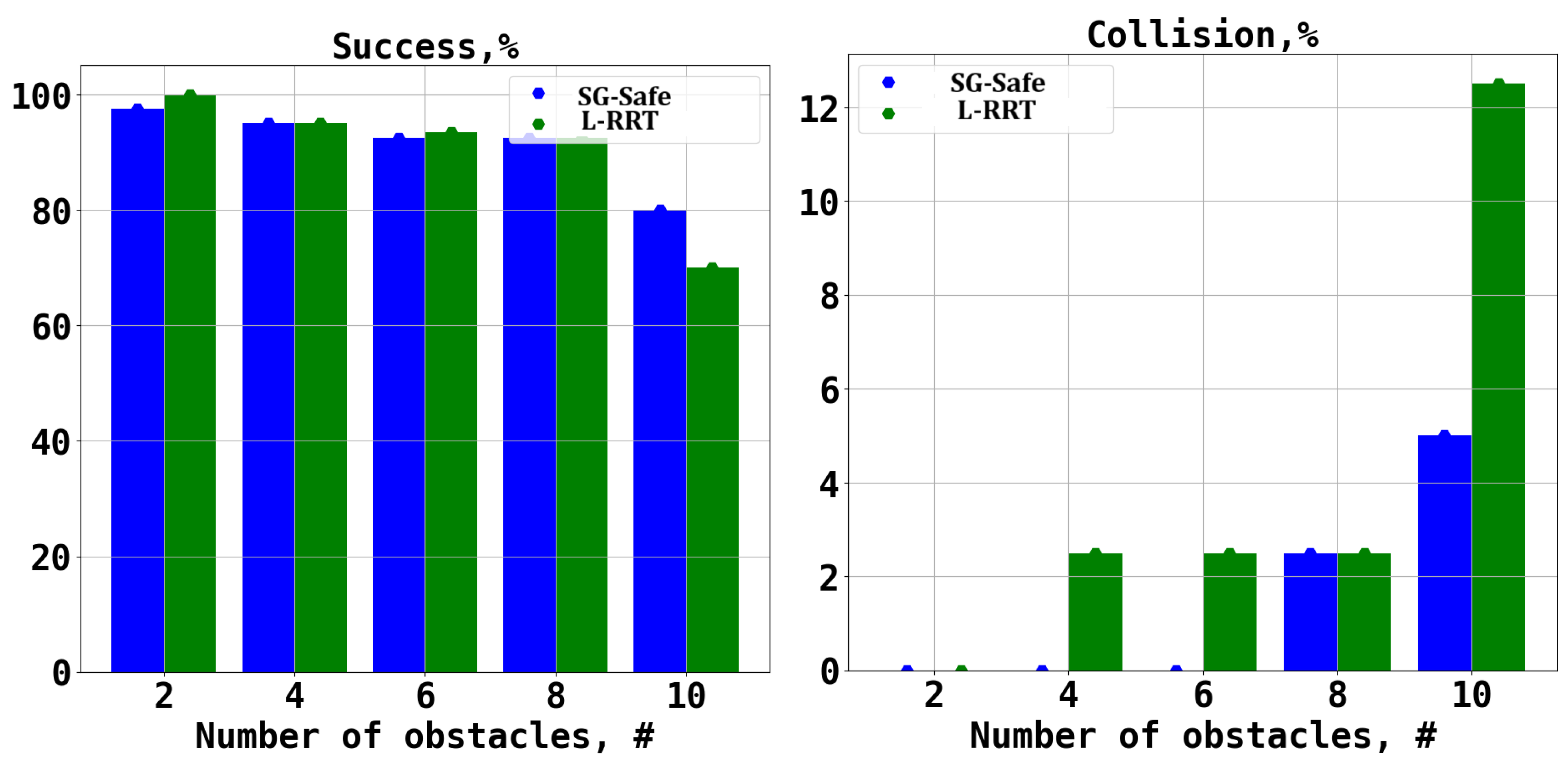
We further analyze scalability by increasing the obstacle density ( N o b s = 2 –10). Figure 4 shows that SG-Safe remains robust, producing zero collisions up to 6 obstacles and outperforming L-RRT, which fails already at 4 obstacles. The gap widens in more complex settings (8–10 obstacles), where SG-Safe maintains higher success due to embedded obstacle awareness and adaptive safety behavior, while L-RRT struggles to find feasible geometric paths through narrow safe zones.
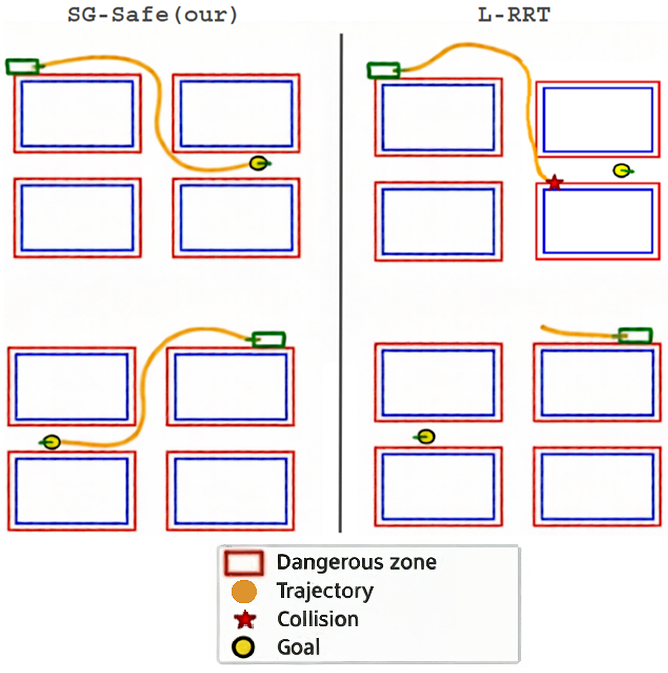
Finally, Table 4 highlights complementary strengths of planning baselines. RRT with Dubins steering can achieve higher success rates but generates trajectories that pass dangerously close to obstacles and supports only kinematic controls ( v , γ ) . L-RRT additionally suffers from kinematic infeasibility in narrow corridors: small regions of attraction require tracking precision beyond the controller’s capability. In contrast, SG-Safe avoids online planning overhead, achieving ∼10× faster inference while keeping competitive success rates, and it attains better time-to-reach (TTR) by directly producing kinodynamically feasible actions ( a , ω ) rather than suboptimal sampled trajectories. Figure A3 illustrates typical corridor failures of L-RRT: planned waypoints can be infeasible to track, leading to collisions or halting when the safety shield blocks the next action, whereas SG-Safe makes consistent safe progress under partial observability without relying on online planning.
SG-Safe incurs additional training-time computation because it optimizes an extra subgoal policy (Equation (8)) alongside the standard safe actor–critic updates using replay batches; this overhead is confined to training and does not affect deployment. At inference time, we discard the subgoal policy and execute only the learned safe low-level policy, so the per-step computation is a single-actor forward pass, comparable to SAC-LAG. In contrast, planning-based baselines additionally incur online planning and tracking costs (e.g., non-zero planning time in Table 4), which our method avoids at deployment.

5.6. RQ3: Comparison with Baselines

5.6.1. Safety Gym Benchmark

Table 2 summarizes performance on Safety Gym. Among learning-based methods, SG-Safe achieves the lowest average collision rate (CR = 0.03) while maintaining a high success rate (SR = 0.87). SAC-LAG attains a slightly lower MTSC, but this is mainly due to overly conservative behavior (the policy often remains stationary), which reduces exposure to hazards at the cost of poor task completion. In contrast, SG-Safe preserves goal-directed behavior and reduces collisions by stopping at safe distances near hazards. We also observe that SG-Safe can outperform SG-NoSafe on some tasks (e.g., Point and Doggo), suggesting that explicitly optimizing safety can improve exploration efficiency by discouraging unsafe detours and repeated recoveries from violations.

5.6.2. POLAMP Benchmark

Results on POLAMP are reported in Table 3 and Table 4. At Level 2, SG-Safe substantially outperforms single-policy Safe RL baselines in terms of success rate (SR = 0.897 vs. 0–0.363) while keeping safety costs low, indicating that the hierarchical structure is critical for long-horizon navigation. We additionally include ADVICE as a prior Safe RL baseline; however, ADVICE (DDPG without HER-style goal relabeling) performs poorly in POLAMP due to the long-horizon sparse-reward setting, yielding near-zero SR. This supports the importance of HER-style relabeling for goal-conditioned navigation, which we therefore adopt in all SAC-based baselines for a fair and stable comparison. In particular, methods based on online filtering or stronger modeling assumptions (e.g., SAC-RCBF) are limited by computational overhead and/or reliance on explicit robot/cost models, whereas cost-penalized single-policy methods (SAC-LAG, SAC) fail to solve Level 2 tasks due to insufficient exploration under constraints.
Variance across seeds mainly comes from stochastic neural network initialization and minibatch/replay sampling in off-policy training (as well as exploration noise). In Safety Gym, additional variance is introduced by randomized initial configurations (goal/hazard placements), while POLAMP is largely deterministic and, thus, seed variance is dominated by optimization stochasticity.
Overall, SG-Safe achieves the best safety–performance trade-off across both benchmarks among end-to-end RL methods, while remaining applicable under the partial-observability and limited-information setting considered in this work.

5.7. RQ4: Component Analysis

5.7.1. Cost Critic Architecture Analysis

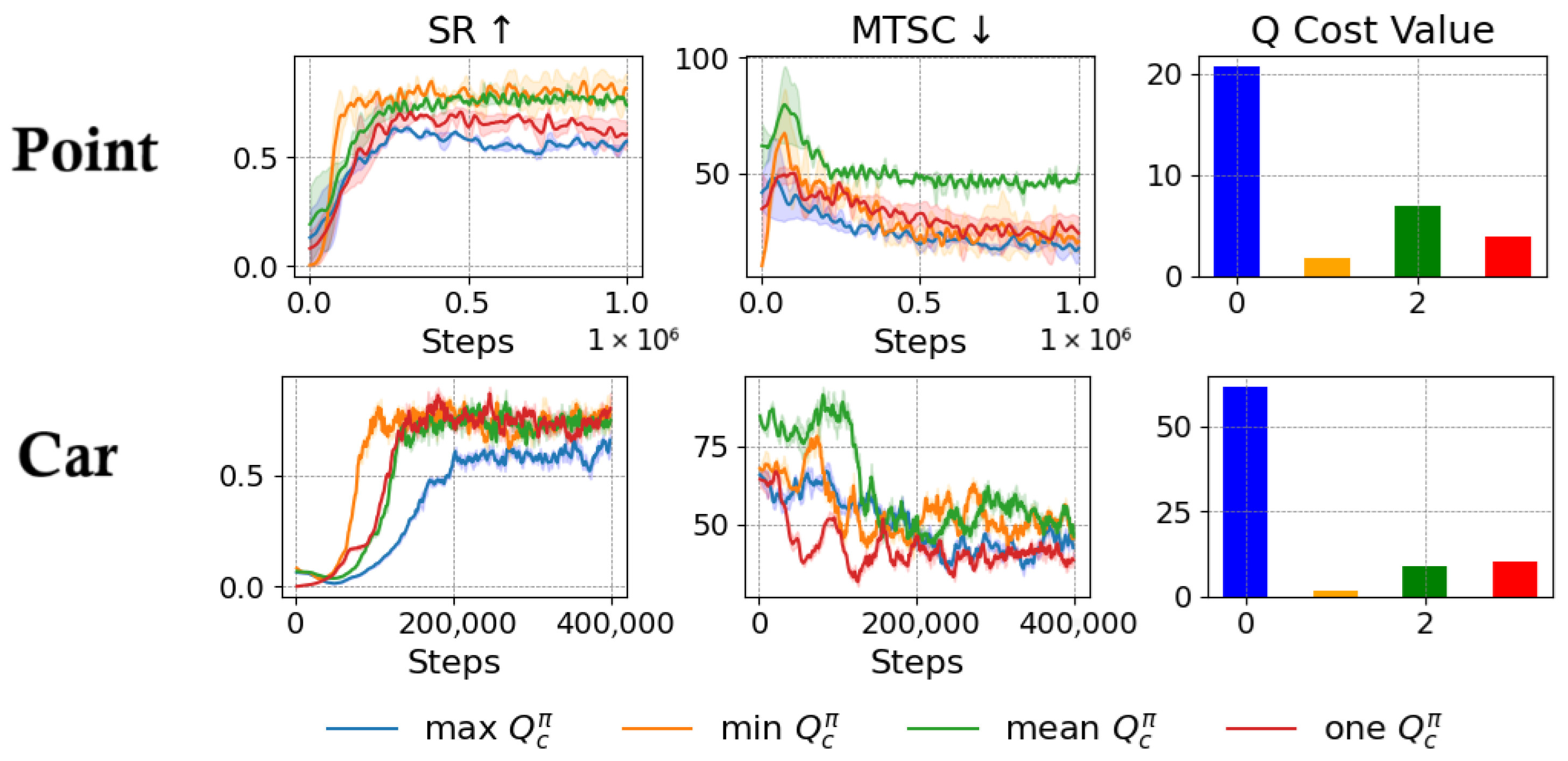
We investigated the SG-Safe algorithm with both single- and dual-cost-critic architectures ( Q c π θ ). To verify the robustness of our results across different configurations, we conducted experiments in the Safety Gym environment using two robots: Point and Car. While the existing literature presents implementations utilizing both single [34] and dual critics [5], the comparative analysis of these architectures remains unexplored.
The results illustrated in Figure 5 demonstrate that employing a single cost critic leads to overestimation of cumulative costs C ( π ) , resulting in a more conservative algorithm that prioritizes safety at the expense of task performance. A similar risk-averse behavior is observed when selecting the maximum value between dual Q-cost critics, where elevated cost estimates drive the policy toward more cautious decisions. Conversely, using two critics and selecting the minimum value produces a less constrained algorithm with improved performance, albeit with reduced overall safety.
Based on our analysis, we adopt the dual-critic architecture with minimum value selection as the default configuration for SG-Safe, as it ensures that the algorithm remains within the prescribed cost limit d while maintaining competitive task performance. This architectural choice represents a significant contribution to the Safe RL methodology, providing empirical guidance for critic architecture selection in constrained Reinforcement Learning problems.

5.7.2. Hyperparameter Sensitivity Analysis

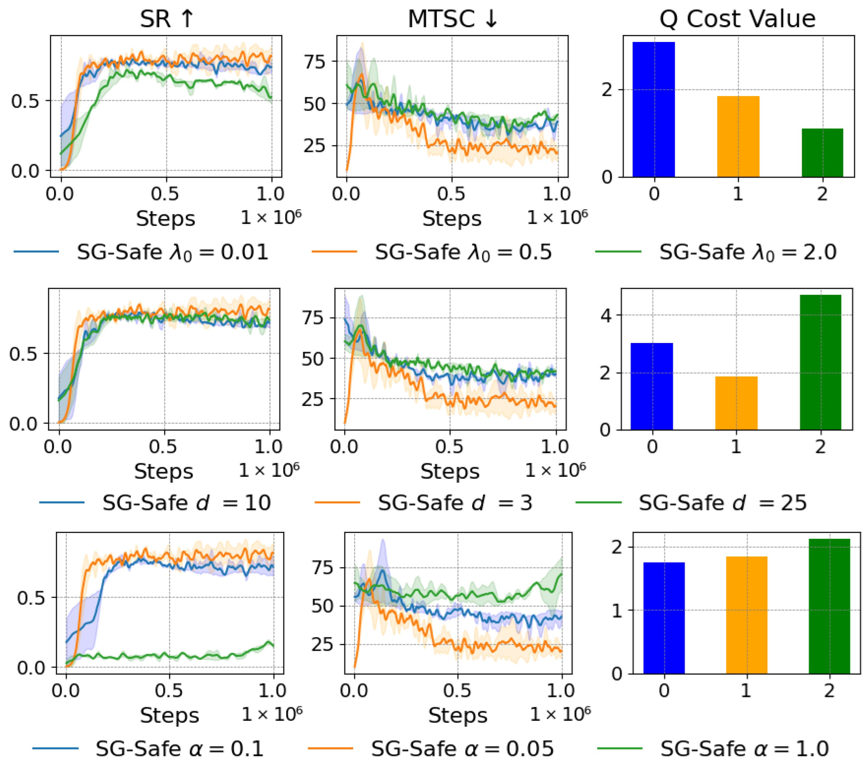
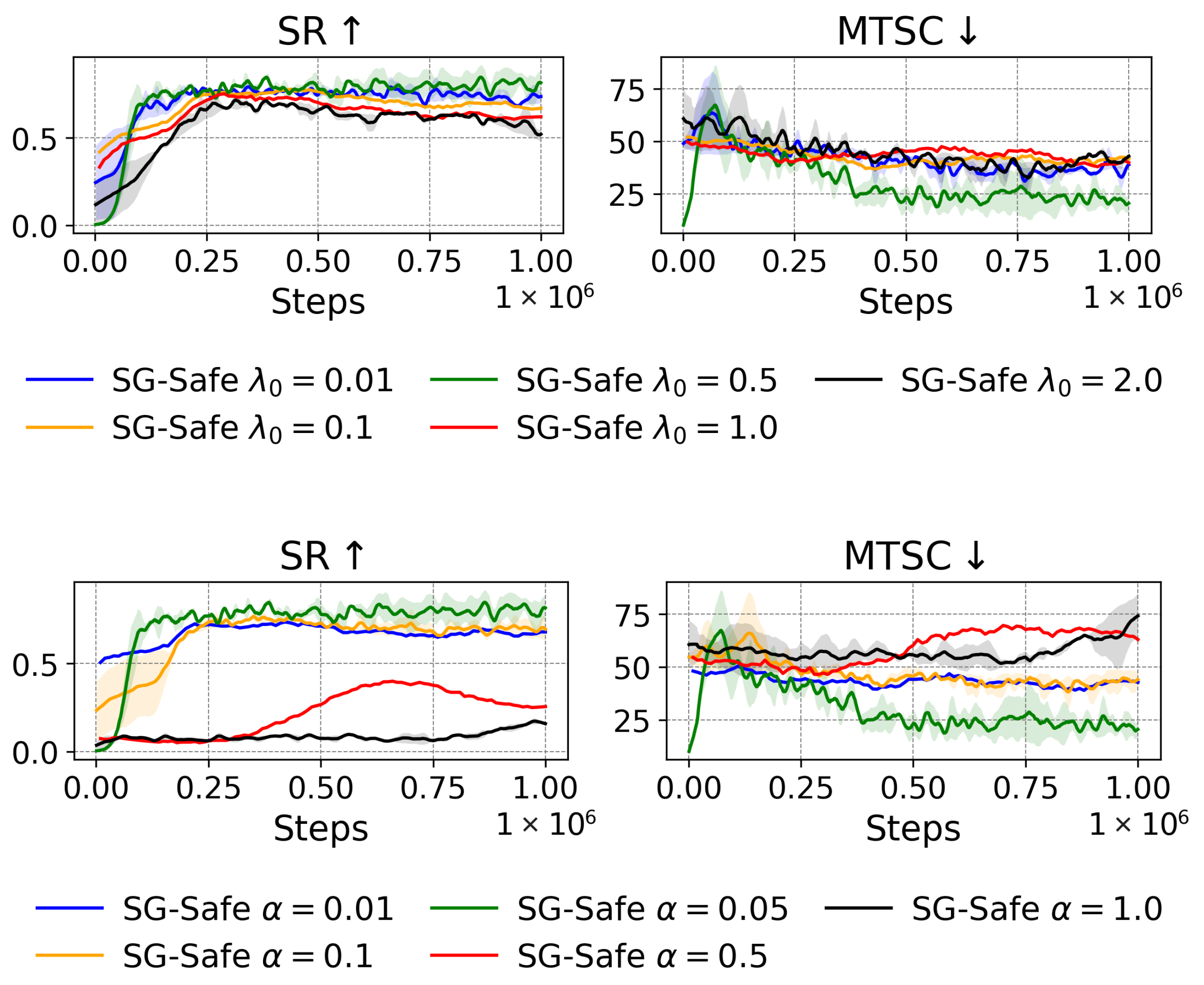
We conducted additional hyperparameter ablation studies (Figure 6) examining three key parameters: α (subgoal policy influence weight), initial λ 0 (safety coefficient), and cost limit d (maximum episode cost).
The analysis reveals that α = 1.0 causes complete learning failure (success rate: 0.2) due to three factors: (1) poor initial subgoal predictions during early training, (2) existence of solvable tasks requiring no subgoals, and (3) forced adherence to inaccurate subgoals leading to local optima. Additional ablation studies visualizing the effects of safe subgoals on learning are provided in the Appendix D.
Key Component Analysis Findings:
  • Cost Critics: Dual critics with min selection provide optimal safety–performance balance.
  • Subgoal Influence ( α ): Lower values ( α < 1.0 ) prevent learning collapse.
  • Safety Coefficient ( λ 0 ): Moderate initialization enables effective constraint learning.
  • Cost Limit (d): Tighter constraints improve safety but reduce task performance.

6. Discussion

SG-Safe shows strong empirical safety–performance trade-offs on Safety Gym and POLAMP, but several limitations and scalability aspects should be noted.
First, SG-Safe is based on SAC-Lagrangian optimization and enforces constraints in expectation during training; it does not provide formal deployment-time guarantees (worst-case or probabilistic). Under partial observability, unknown dynamics, and function approximation, such guarantees would require additional assumptions (e.g., certified state estimation, bounded/known dynamics, or conservative model uncertainty). Therefore, residual risk may appear under distribution shift, out-of-distribution observations, or strong perception noise. In contrast, methods such as CBF/SafetyLayer can provide formal guarantees under stronger modeling assumptions.
Second, SG-Safe assumes that training data covers safety-critical scenarios; changes in dynamics, sensing, or safety definitions at deployment can degrade safety.
Third, we observed several practical failure modes. (i) Sensitivity to Subgoal Influence α : Overly large α can over-constrain the low-level policy early in training and lead to learning collapse (see the α sweep in Figure 6/Appendix E), because subgoals are inaccurate before the safe policy has learned meaningful behavior. (ii) Potential Over-Reliance on Subgoals: If the subgoal policy is misaligned, the low-level policy may become overly cautious or stall in narrow passages (a common failure pattern in the hardest POLAMP Level-2 layouts; Table 3). Remedies: In our experiments, stable performance was obtained with small α ; more generally, we recommend (a) a warm-up/annealing schedule for α , (b) confidence-gated or advantage-gated subgoal guidance (disable KL guidance when it degrades the critic-estimated objective), and (c) subgoal dropout to reduce dependence on the high-level module. For additional robustness, noise augmentation during training improves deployment under noisy observations (Appendix C), and future work could incorporate lightweight feasibility checks (e.g., kinematic consistency filters) or short-horizon rollouts to reject clearly infeasible subgoals before applying subgoal guidance.
Regarding scalability, inference cost is a single-actor forward pass and scales similarly to standard actor–critic methods with state/action dimensionality. For higher-dimensional observations (e.g., images), SG-Safe can be applied by replacing the MLP encoder with a vision backbone. Subgoals can be generated in the learned latent space, so the hierarchical mechanism remains unchanged. For multiple safety constraints, a standard Lagrangian extension applies by training one cost critic per constraint and optimizing a vector of multipliers.
Future work could include uncertainty-aware modeling and hybrid designs that combine training-time-constrained optimization with lightweight runtime monitoring, as well as model-based components (e.g., short-horizon rollouts in latent space) to improve long-horizon planning under complex constraints while keeping deployment overhead low.

7. Conclusions

We proposed SG-Safe, a hierarchical RL method that enhances safe exploration in long-horizon navigation through subgoal guidance. Unlike existing approaches, SG-Safe operates without full observability or explicit cost function knowledge, and it relies on a single policy during inference for computational efficiency.
Across Safety Gym and POLAMP, SG-Safe consistently achieves a strong safety–performance trade-off compared to evaluated end-to-end Safe RL baselines under partial observability, while maintaining substantially lower inference costs than planning-based methods in our setup.
Future work will focus on simplifying the architecture and exploring Sim-to-Real transfer.

Author Contributions

Conceptualization, G.G. and A.P.; methodology, G.G.; software, G.G.; formal analysis, G.G.; investigation, G.G.; writing—original draft preparation, G.G.; writing—review and editing, G.G. and A.P.; supervision, A.P. All authors have read and agreed to the published version of the manuscript.

Funding

The study was supported by the Ministry of Economic Development of the Russian Federation (agreement No. 139-15-2025-013, dated 20 June 2025, IGK 000000C313925P4B0002).

Institutional Review Board Statement

Not applicable.

Informed Consent Statement

Not applicable.

Data Availability Statement

The source code supporting the findings of this study is available at https://github.com/Gricha1/SPEIS, accessed on 8 February 2026.

Conflicts of Interest

The authors declare no conflicts of interest.

Appendix A. Safety Gym Benchmark Configuration

The Safety Gym environment utilizes a procedurally generated 4 m × 4 m arena containing eight circular hazard obstacles. Both obstacle placements and task configurations (start and goal states) are randomly regenerated at the start of each episode. Task generation ensures collision-free initialization by verifying that the robot’s inflated bounding volume does not intersect with any hazards in both the start and goal configurations. This problem formulation follows the established benchmark setup described in [10].
We evaluated our method using four distinct robotic platforms available in Safety Gym, each with different kinematic properties and complexity levels:
  • Point: A simple differential drive robot with 2D navigation capabilities.
  • Car: An Ackermann-steering vehicle with realistic turning constraints.
  • Doggo: A quadruped robot with complex leg coordination requirements.
  • Sweeps: A holonomic platform with omnidirectional movement capabilities.
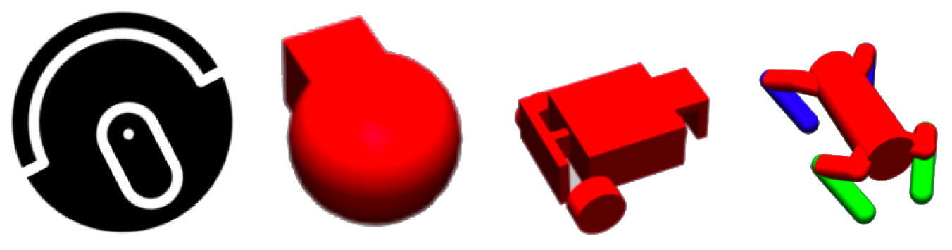
The detailed specifications of each robot’s observation and action space dimensions are provided in Table A1, while visual representations of each platform are shown in Figure A1. All agents receive proprioceptive state information (joint positions, velocities) and exteroceptive lidar-like observations detecting proximity to static hazards and goal locations. The observation space is goal-conditioned, concatenating the current agent state with the target goal vector.
The reward structure incorporates both time penalties and success incentives: Agents receive a constant penalty of r t = 1 for each time step, encouraging efficient navigation. Additionally, they obtain a substantial success bonus of r s u c c e s s = 10 upon reaching the goal (defined as Euclidean distance e p 0.3 m). Episode termination occurs immediately if the agent enters any hazard zone, at which point the agent additionally receives a collision penalty of r = 100 .
The cost function implements safety constraints through zone-based penalties: agents receive a unit cost ( c = 1 ) when entering the buffer zone surrounding hazards, which represents the safety margin where proximity to danger is penalized. We set the safety constraint threshold (cost limit) to d = 3.0 across all Safety Gym experiments. This buffer zone typically extends beyond the actual hazard boundary to promote conservative navigation behavior, consistent with the safety constraints formulation in [10].
Figure A1. Robot embodiments from Safety Gym: Sweeps, Point, Car, and Doggo.
Technologies 14 00146 g0a1
Table A1. Action and state space dimensions across POLAMP and Safety Gym benchmarks.
BenchmarkRobotAction DimState Dim
POLAMPVehicle288
Safety GymPoint228
Safety GymCar242
Safety GymDoggo12108
Safety GymSweeps24

Appendix B. POLAMP Benchmark

The POLAMP benchmark utilizes a static 40 m × 40 m environment featuring challenging narrow corridors. The agent receives a reward of −1 for every step and a penalty of −100 for colliding with an obstacle, which also terminates the episode. In the POLAMP benchmark, we set the safety constraint threshold (cost limit) to d = 3.0 . Additionally, we impose an immediate constraint cost as c i ( s i , a i , g i ) = l m i n r s a f e t y , where r s a f e t y = 0.3 m is the safety radius and l m i n is the minimum current lidar signal (or the minimum distance to obstacles for environments without lidars).
We set the safety radius to r s a f e t y = 0.3 m as a conservative clearance margin consistent with the POLAMP benchmark convention and the vehicle footprint/partial-observability uncertainty. Changing r s a f e t y simply tightens or relaxes the constraint (larger values are more conservative, typically lowering SR and increasing TTR while reducing collision risk, and smaller values do the opposite).
We developed two distinct datasets with varying complexity levels to evaluate navigation capabilities under different constraints.
Level 1 comprises simpler navigation tasks requiring at most one directional change within corridor constraints, with start–goal distances ranging from 10 to 20 m. Level 2 presents substantially more complex challenges, requiring agents to execute two precise turns in narrow corridors to reach destinations spaced 20–30 m apart.
The dataset generation employed systematic pattern-based sampling: 30 distinct path configurations for Level 1 and 12 more challenging patterns for Level 2. Each dataset contains 96 unique tasks with specifically designed start–goal state pairs that ensure kinematic feasibility while testing navigation precision. Representative examples of both difficulty levels are illustrated in Figure A2.
Figure A2. Dataset navigation patterns. The vehicle’s initial position and orientation are shown as a green rectangle, with the goal position indicated by a yellow circle. (Left): Representative Level 1 pattern requiring at most one directional change. (Right): Representative Level 2 pattern requiring two precise turns in narrow corridors.
Technologies 14 00146 g0a2
Figure A3. Comparison of navigation trajectories generated by SG-Safe (ours) and L-RRT on the POLAMP benchmark.
Technologies 14 00146 g0a3

Appendix C. Robustness to Observation and Action Noise

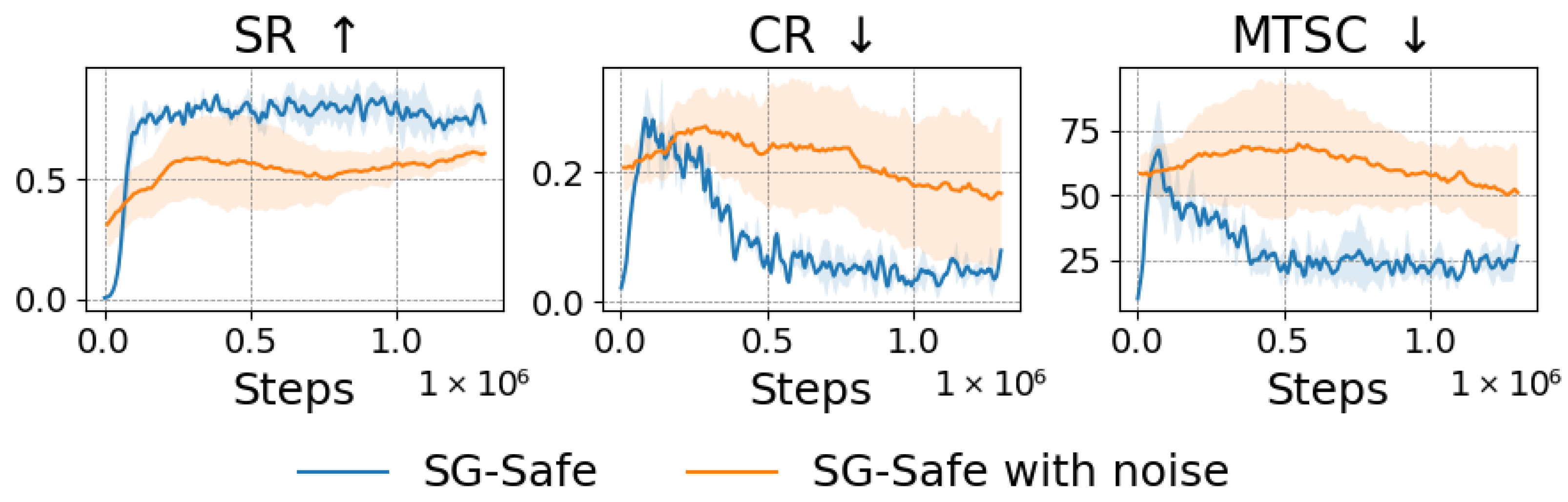
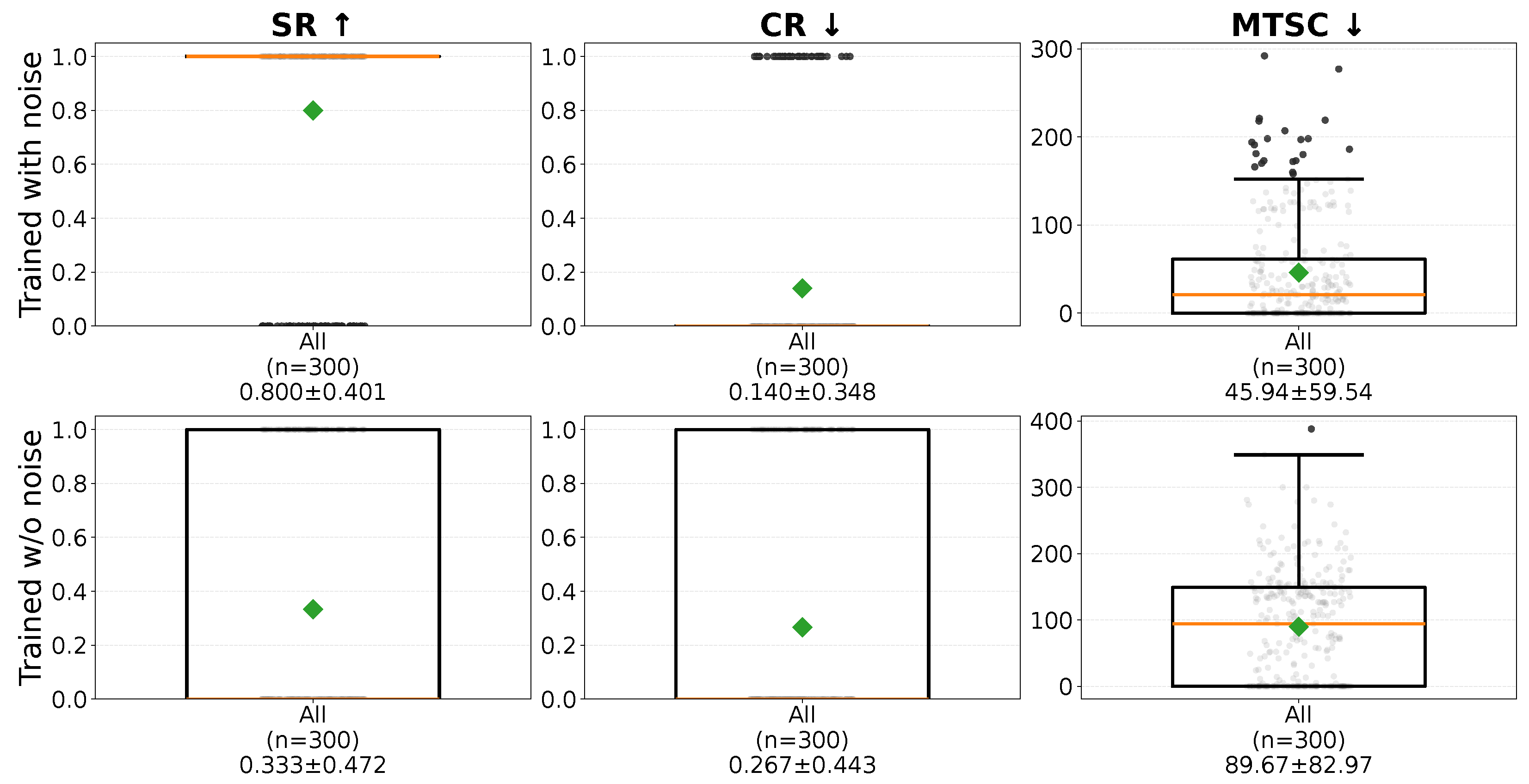
To evaluate robustness under realistic sensing and actuation disturbances, we tested SG-Safe in a setting where both observations and actions were corrupted by noise at execution time. We trained SG-Safe on the Safety Gym Point environment with zero-mean Gaussian noise ( σ = 0.1 ) applied to both observations and actions during experience collection. We compared (i) SG-Safe trained without noise (standard training) and evaluated under noisy observations/actions, and (ii) SG-Safe trained with noise augmentation, where we injected the same type of noise into observations and actions during training (data augmentation). Figure A4 shows the corresponding learning curves (training without noise vs. with noise augmentation). Table A2 reports the mean ± std over multiple seeds under the noisy evaluation setting, demonstrating that noise-augmented training substantially improves stability and safety–efficiency. Figure A5 further visualizes the per-episode metric distributions as box plots (pooled over all episodes), highlighting that noise augmentation consistently shifts the distributions toward higher success and lower collisions/cost.
Table A2. Noise robustness under noisy evaluation (observation and action noise applied at execution). “Trained without noise” denotes a policy trained in the clean setting but evaluated under noise. “Trained with noise augmentation” injects the same type of noise into observations/actions during training. Results are reported as the mean ± std across five seeds.
SG-Safe Training SettingSR↑CR↓MTSC↓
Trained with noise augmentation 0.78 ± 0.03 0.13 ± 0.03 47.80 ± 3.60
Trained without noise (tested with noise) 0.34 ± 0.03 0.22 ± 0.02 83.00 ± 13.59
Figure A4. Training curves under (left) clean training and (right) noise-augmented training. Both were evaluated with observation/action noise during experience collection.
Technologies 14 00146 g0a4
Figure A5. Noise robustness under noisy execution. Box plots show the distribution of per-episode metrics over all evaluation rollouts (All: n = 300 , pooled across 3 seeds × 100 tasks). Green diamonds indicate the mean; darker points denote outliers; Orange line inside each box indicates the median (1.5 × IQR). Top row: trained with noise augmentation. Bottom row: trained without noise (tested with noise).
Technologies 14 00146 g0a5

Appendix D. Ablation Experiments/Safety Subgoals

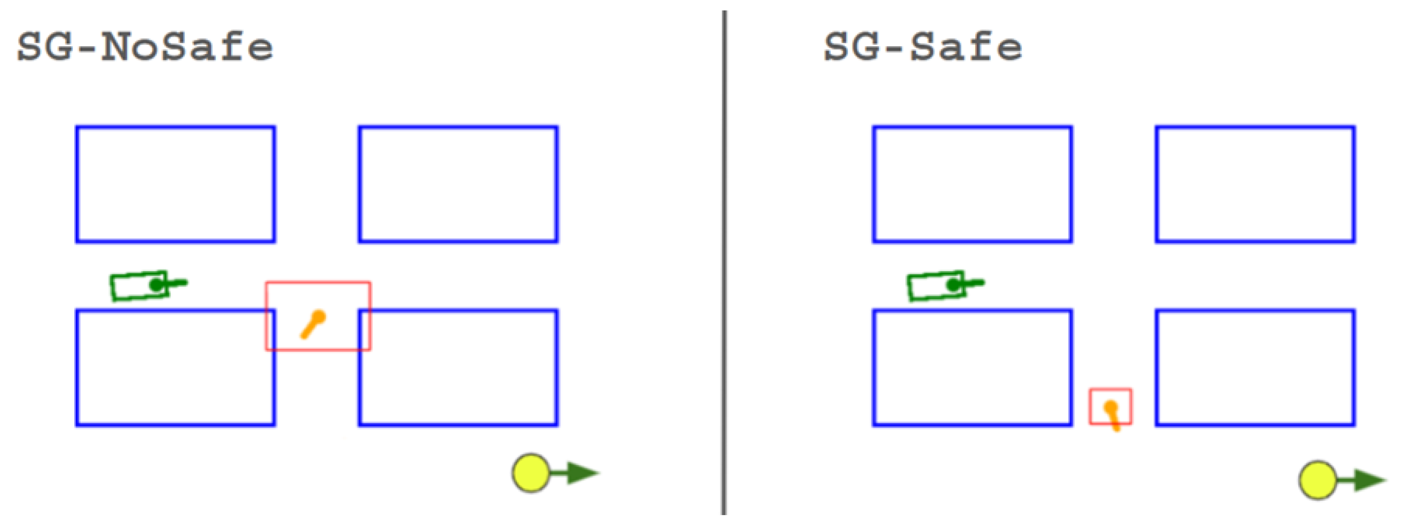
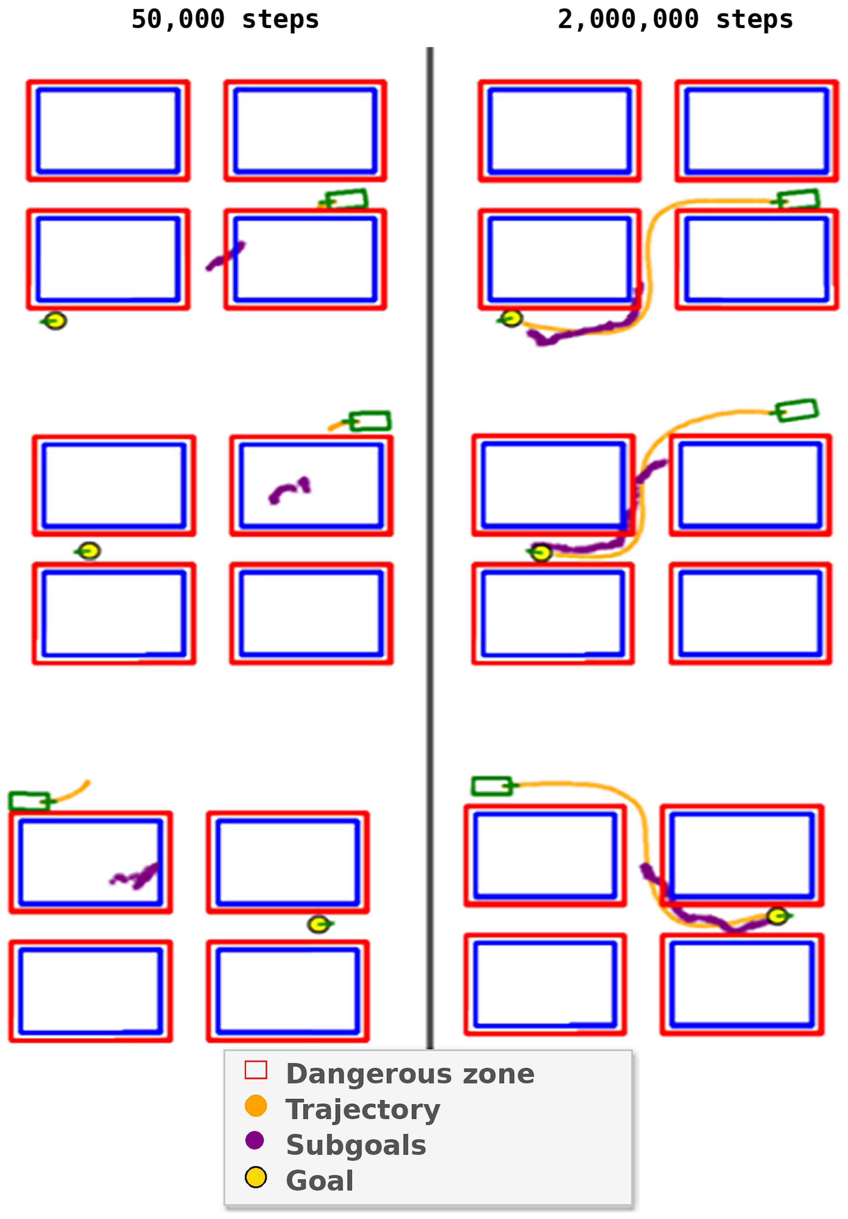
We observed that the subgoal policy becomes safer over training. Figure A6 and Figure A7 show that subgoal samples shift away from hazardous regions from early training to convergence. This behavior emerges because the subgoal policy is trained by KL-divergence minimization toward the agent’s state visitation distribution: as the low-level safe policy improves constraint satisfaction, the visitation distribution shifts toward safer regions, and the subgoal policy co-adapts accordingly, without explicit safety supervision at the subgoal level.
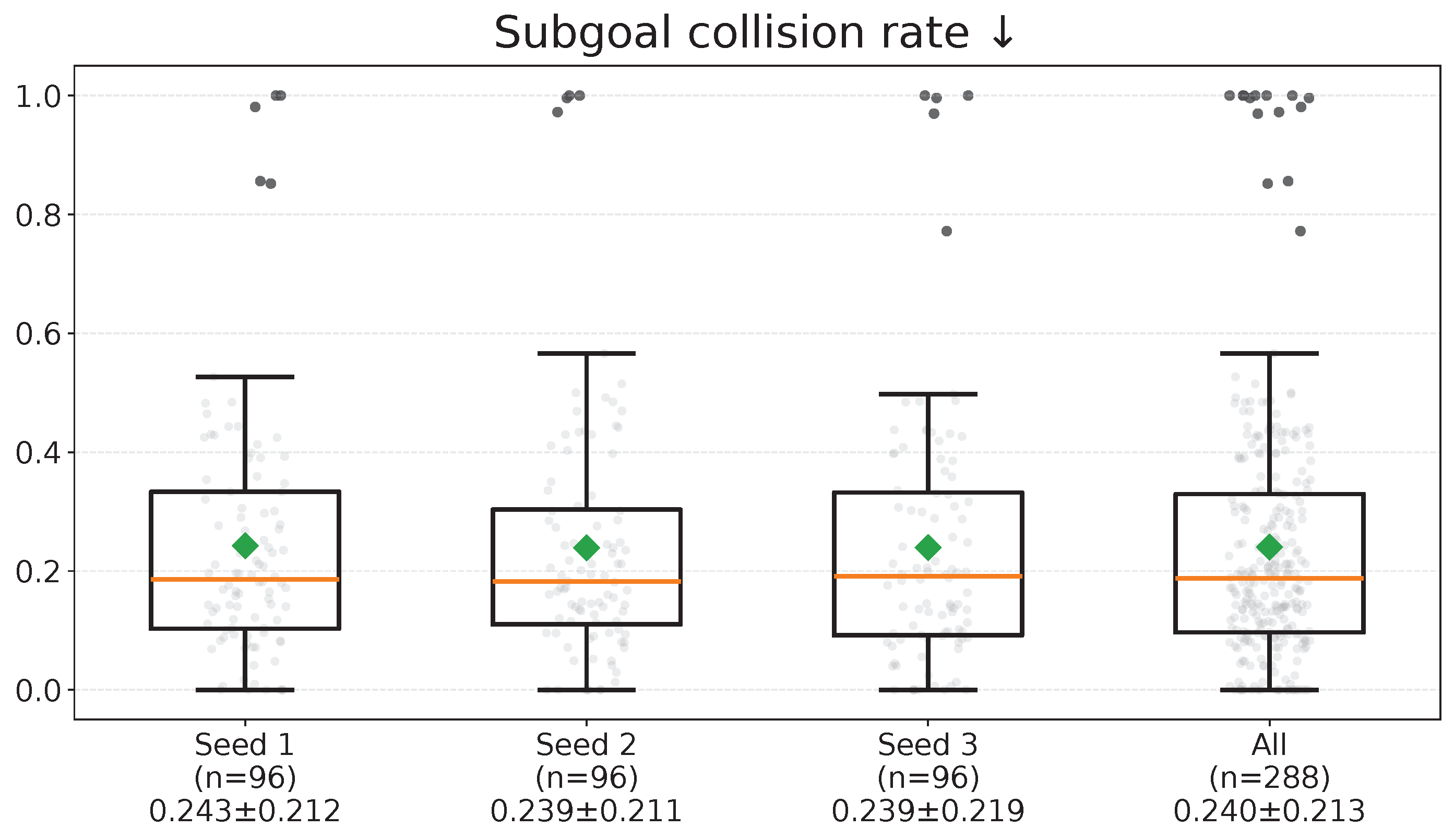
To quantify this effect, we measured the subgoal collision rate (i.e., fraction of generated subgoals located inside or within the safety margin of hazardous regions). As summarized in Table A3, across three seeds, the collision rate decreased from an early-training mean of 0.63 (values: 0.80, 0.53, 0.55) to 0.23 at convergence (values: 0.243, 0.239, 0.239), corresponding to an approximately 2.7× reduction in unsafe subgoal proposals. This quantitatively supports the qualitative visualization shown in Figure A6.
Figure A6. Comparison of subgoal generation between SG-NoSafe (Left) and SG-Safe (Right). Orange arrows indicate mean subgoal positions (x,y coordinates), with rectangles representing standard deviation regions, yellow—goal, green—agent, blue—obstacles. SG-Safe generates safer subgoals with lower positional variance due to safety constraints.
Technologies 14 00146 g0a6
Importantly, we do not claim that this is an intrinsic or guaranteed property of the method. Rather, it is an empirical phenomenon that arises when (i) the low-level policy successfully learns safe behavior and (ii) the KL-based alignment term is used. Under significantly different reward or cost definitions, or if the safe policy fails to learn meaningful constraint satisfaction, this effect may weaken or disappear.
We also empirically observed cases where the subgoal policy proposes states that are safe but dynamically infeasible or lead to local dead ends. In SG-Safe, subgoals are treated as soft guidance rather than hard constraints. The goal-conditioned policy is not required to exactly reach the subgoal; instead, the KL term only biases the policy distribution. In practice, this allows the policy to deviate from unhelpful subgoals while still optimizing the reward–cost trade-off. Such cases occur mainly in early training and become less frequent as the subgoal distribution aligns with feasible safe trajectories.
These results provide quantitative interpretability of the subgoal policy and support the claim that subgoals become safer during training in our setting, while clearly framing this as an empirical observation rather than a formal guarantee.
Table A3. Subgoal collision rate of SG-Safe at early training (50k steps) and at the end of training (2M steps), aggregated over 3 seeds (lower is better).
Early (50k)End (2M)
Mean ± Std (across seeds)0.627 ± 0.1500.240 ± 0.002
To further characterize variability beyond the seed-averaged summary in Table A3, we additionally report the episode-level distribution of the subgoal collision rate at convergence. Figure A8 shows box plots over the 96 evaluation tasks for each seed (total 288 episodes), as well as the pooled distribution across all seeds. The box indicates the interquartile range (IQR) with the median, whiskers extend to 1.5×IQR, and markers denote the mean; semi-transparent dots show individual episode values. This visualization confirms that the reduction in unsafe subgoal proposals is consistent across tasks and seeds, rather than being driven by a small subset of episodes.
Figure A7. Evolution of subgoal policy during SG-Safe training. (Left): Subgoals sampled at early training (50k steps). (Right): Subgoals after convergence (2M steps). Purple markers denote generated subgoals, orange curves show the executed trajectories, red rectangles indicate hazardous regions, and the yellow marker denotes the final goal. Over training, the subgoal distribution shifts away from hazards and becomes better aligned with safe trajectory visitation. Green marker denotes the agent position.
Technologies 14 00146 g0a7
Figure A8. Episode-level distribution of the subgoal collision rate at convergence (2M steps). We show per-seed distributions over 96 evaluation tasks (box plots) and the pooled distribution across all seeds (All). Boxes denote IQR with median; whiskers extend to 1.5×IQR; green diamonds denote the mean; dots are individual episodes, diamonds; orange line inside each box indicates the median.
Technologies 14 00146 g0a8

Appendix E. Training Details

Quick-Start and Environment Configuration Summary

  • Code and Branches:
Our implementation is publicly available at https://github.com/Gricha1/SPEIS (accessed on 8 February 2026). We provide two entry points matching the two benchmarks used in this paper: (i) SAFETY_GYM branch for Safety Gym experiments, and (ii) the POLAMP branch (default) for POLAMP experiments.
  • Quick-Start (High-Level):
  • # 1) Get code
    git clone https://github.com/Gricha1/SPEIS.git
    cd~SPEIS
  • # 2) Select benchmark
    git checkout SAFETY_GYM        # Safety Gym experiments
    # OR keep default branch        # POLAMP~experiments
  • # 3) Install dependencies (see repository README/requirements)
    # (create conda/venv, then install requirements)
  • # 4) Run training/evaluation
    # Use the provided training/eval entrypoints in the repository README.
    # Recommended: run 3--5 seeds and report mean ± std for SR/CR/MTSC.
  • Subgoal Visualization (Built-in):
To support qualitative inspection of the subgoal policy, our implementation already logs and visualizes sampled subgoals during training/validation runs (together with the executed trajectory and hazardous regions). In particular, enabling trajectory plotting (e.g., via the provided validation/training scripts) produces per-episode PNG frames that overlay sampled subgoals; we also provide a helper utility (utilite_video_generator.py) to convert the saved frames into a single video/figure artifact for convenient inspection and reproduction of Figure A3-style visualizations.
For policy training in SG-Safe, we employ the HER buffer [27] to address sparse reward challenges. HER leverages the insight that even when the original goal is not achieved, other goals might have been reached during episode rollouts. This enables the creation of virtual transitions through goal relabeling, where the original goal is replaced with alternative goals sampled from the replay buffer. We adopt the goal relabeling strategy from the original HER implementation:
  • 20% of transitions retain their original goals;
  • 40% use randomly sampled states from other trajectories in the replay buffer;
  • 40% use future states from the same trajectory.
We further analyzed the sensitivity of SG-Safe to hyperparameter choices using a broader sweep in Safety Gym (Point). This study is intended to address whether the method admits robust default settings, and to identify failure modes that practitioners should avoid. Unless stated otherwise, each configuration was evaluated over multiple random seeds, and we report both success (SR) and safety-related metrics (MTSC/cost statistics).
Figure A9. Extended hyperparameter sweep for SG-Safe in Safety Gym (Point). Each curve corresponds to a different hyperparameter configuration; shaded regions indicate variation across seeds. The figure complements Figure 6 by covering a wider range of settings and highlighting both stable regions and failure modes.
Technologies 14 00146 g0a9
  • Observed Stability Patterns: Across the sweep, SG-Safe exhibits a relatively stable operating region where performance and safety trade-offs change smoothly with hyperparameters, suggesting that the method is not overly brittle. The most sensitive parameter is the subgoal influence weight α : very large values can over-constrain the low-level policy early in training, effectively forcing it to follow inaccurate subgoals and resulting in convergence to poor local solutions or learning collapse. This failure mode is consistent with the degradation observed at α = 1.0 in Figure 6.
  • Recommended Default Ranges: Based on the sweep results, we recommend using moderate subgoal influence ( α 1 ) and moderate λ 0 initialization, while tuning the cost limit d according to the desired safety strictness. In our benchmarks, these defaults generalize across Safety Gym and POLAMP without requiring environment-specific redesign of the algorithmic components. We emphasize that tighter d reliably improves safety at the expense of task completion, whereas overly aggressive α is the primary cause of instability.
  • Seed-Level Robustness: We also observed that, within the stable hyperparameter region, performance differences across seeds were substantially smaller than the gaps between stable versus unstable regimes. Therefore, the main practical guidance is to avoid extreme subgoal forcing and to use moderate safety multiplier initialization; once within this region, SG-Safe behaves predictably across random seeds and task variants.
The complete hyperparameter configurations for both the Safety Gym and POLAMP environments are provided in Table A4, including environment-specific adjustments and optimization parameters.
Table A4. Complete hyperparameter configurations for both Safety Gym and POLAMP environments, including environment-specific adjustments and optimization parameters.
HyperparameterPOLAMPSafetyGym
Encoder Parameters
Learning rate 0.0001
Batch size2048
Embedding dim256
Hidden dim128
ϵ k 1.0
δ 0.2
Subgoal Policy (High-Level SAC) Parameters
Actor learning rate 0.0001 0.0001
Reward critic learning rate 0.001 0.001
N critics (reward)22
Hidden dim256256
α 0.05 0.05
ϵ 0.05 0.05
N ensemble2020
clip v 150 150
Batch size20482048
Soft update rate 0.005 0.005
γ 0.99 0.99
Safe Policy (Low-Level SAC) Parameters
Actor learning rate 0.0001 0.0001
Reward critic learning rate 0.001 0.001
Cost critic learning rate 0.001 0.001
N critics (reward, cost)22
Hidden dim256256
Batch size20482048
Soft update rate 0.005 0.005
λ i n i t 0.5 0.5
λ Learning rate 0.0005 0.0005
λ Update freq10001000
Cost limit 3.0 3.0

References

  1. Zhu, Z.; Zhao, H. A survey of deep rl and il for autonomous driving policy learning. IEEE Trans. Intell. Transp. Syst. 2021, 23, 14043–14065. [Google Scholar] [CrossRef] [Scilit]
  2. Ha, S.; Xu, P.; Tan, Z.; Levine, S.; Tan, J. Learning to walk in the real world with minimal human effort. arXiv 2020, arXiv:2002.08550. [Google Scholar] [CrossRef] [Scilit]
  3. Gu, S.; Yang, L.; Du, Y.; Chen, G.; Walter, F.; Wang, J.; Knoll, A. A Review of Safe Reinforcement Learning: Methods, Theories and Applications. IEEE Trans. Pattern Anal. Mach. Intell. 2024, 46, 11216–11235. [Google Scholar] [CrossRef] [Scilit] [PubMed]
  4. Altman, E. Constrained Markov Decision Processes; CRC Press: Boca Raton, FL, USA, 1999; Volume 7. [Google Scholar]
  5. Chow, Y.; Ghavamzadeh, M.; Janson, L.; Pavone, M. Risk-constrained reinforcement learning with percentile risk criteria. J. Mach. Learn. Res. 2017, 18, 6070–6120. [Google Scholar]
  6. Ray, A.; Achiam, J.; Amodei, D. Benchmarking safe exploration in deep reinforcement learning. arXiv 2019, arXiv:1910.01708. [Google Scholar]
  7. Yang, Q.; Simão, T.D.; Tindemans, S.H.; Spaan, M.T. WCSAC: Worst-case soft actor critic for safety-constrained reinforcement learning. In Proceedings of the AAAI Conference on Artificial Intelligence, Virtual, 2–9 February 2021; Volume 35, pp. 10639–10646. [Google Scholar]
  8. Chane-Sane, E.; Schmid, C.; Laptev, I. Goal-conditioned reinforcement learning with imagined subgoals. In Proceedings of the International Conference on Machine Learning, PMLR, Virtual, 18–24 July 2021; pp. 1430–1440. [Google Scholar]
  9. Roza, F.S.; Rasheed, H.; Roscher, K.; Ning, X.; Günnemann, S. Safe Robot Navigation Using Constrained Hierarchical Reinforcement Learning. In Proceedings of the 2022 21st IEEE International Conference on Machine Learning and Applications (ICMLA), Nassau, Bahamas, 12–14 December 2022; pp. 737–742. [Google Scholar]
  10. Xiong, Z.; Eapper, J.; Qureshi, A.H.; Jagannathan, S. Model-free neural lyapunov control for safe robot navigation. In Proceedings of the 2022 IEEE/RSJ International Conference on Intelligent Robots and Systems (IROS), Kyoto, Japan, 23–27 October 2022; pp. 5572–5579. [Google Scholar]
  11. De Heuvel, J.; Shi, W.; Zeng, X.; Bennewitz, M. Subgoal-driven navigation in dynamic environments using attention-based deep reinforcement learning. In Proceedings of the 2023 21st International Conference on Advanced Robotics (ICAR), Abu Dhabi, United Arab Emirates, 5–8 December 2023; pp. 79–85. [Google Scholar]
  12. Zhu, W.; Hayashibe, M. A hierarchical deep reinforcement learning framework with high efficiency and generalization for fast and safe navigation. IEEE Trans. Ind. Electron. 2022, 70, 4962–4971. [Google Scholar] [CrossRef] [Scilit]
  13. Karimpanal, T.G.; Rana, S.; Gupta, S.; Tran, T.; Venkatesh, S. Learning transferable domain priors for safe exploration in reinforcement learning. In Proceedings of the 2020 International Joint Conference on Neural Networks (IJCNN), Glasgow, UK, 19–24 July 2020; pp. 1–10. [Google Scholar]
  14. Angulo, B.; Panov, A.; Yakovlev, K. Policy Optimization to Learn Adaptive Motion Primitives in Path Planning with Dynamic Obstacles. IEEE Robot. Autom. Lett. 2022, 8, 824–831. [Google Scholar] [CrossRef] [Scilit]
  15. Gu, S.; Yang, L.; Du, Y.; Chen, G.; Walter, F.; Wang, J.; Yang, Y.; Knoll, A. A review of safe reinforcement learning: Methods, theory and applications. arXiv 2022, arXiv:2205.10330. [Google Scholar] [CrossRef] [Scilit] [PubMed]
  16. Liu, Y.; Halev, A.; Liu, X. Policy learning with constraints in model-free reinforcement learning: A survey. In Proceedings of the The 30th International Joint Conference on Artificial Intelligence (IJCAI), Virtual, 19–26 August 2021; pp. 4508–4515. [Google Scholar]
  17. Zanger, M.A.; Daaboul, K.; Zöllner, J.M. Safe continuous control with constrained model-based policy optimization. In Proceedings of the 2021 IEEE/RSJ International Conference on Intelligent Robots and Systems (IROS), Prague, Czech Republic, 27 September–1 October 2021; pp. 3512–3519. [Google Scholar]
  18. Dalal, G.; Dvijotham, K.; Vecerik, M.; Hester, T.; Paduraru, C.; Tassa, Y. Safe exploration in continuous action spaces. arXiv 2018, arXiv:1801.08757. [Google Scholar] [CrossRef] [Scilit]
  19. Emam, Y.; Notomista, G.; Glotfelter, P.; Kira, Z.; Egerstedt, M. Safe reinforcement learning using robust control barrier functions. arXiv 2022, arXiv:2110.05415. [Google Scholar] [CrossRef] [Scilit]
  20. Hunt, N.; Fulton, N.; Magliacane, S.; Hoang, T.N.; Das, S.; Solar-Lezama, A. Verifiably safe exploration for end-to-end reinforcement learning. In Proceedings of the 24th International Conference on Hybrid Systems: Computation and Control, Nashville, TN, USA, 19–21 May 2021; pp. 1–11. [Google Scholar]
  21. Yang, W.C.; Marra, G.; Rens, G.; De Raedt, L. Safe Reinforcement Learning via Probabilistic Logic Shields. In Proceedings of the Thirty-Second International Joint Conference on Artificial Intelligence, IJCAI-23; Elkind, E., Ed.; International Joint Conferences on Artificial Intelligence Organization: Palo Alto, CA, USA, 2023; pp. 5739–5749. [Google Scholar]
  22. Bethell, D.; Gerasimou, S.; Calinescu, R.; Imrie, C. Safe reinforcement learning in black-box environments via adaptive shielding. arXiv 2024, arXiv:2405.18180. [Google Scholar] [CrossRef] [Scilit]
  23. Levy, A.; Platt, R.; Saenko, K. Hierarchical actor-critic. arXiv 2017, arXiv:1712.00948. [Google Scholar]
  24. Nachum, O.; Gu, S.S.; Lee, H.; Levine, S. Data-efficient hierarchical reinforcement learning. Adv. Neural Inf. Process. Syst. 2018, 31, 3307–3317. [Google Scholar]
  25. Zhang, T.; Guo, S.; Tan, T.; Hu, X.; Chen, F. Generating adjacency-constrained subgoals in hierarchical reinforcement learning. Adv. Neural Inf. Process. Syst. 2020, 33, 21579–21590. [Google Scholar]
  26. Gürtler, N.; Büchler, D.; Martius, G. Hierarchical reinforcement learning with timed subgoals. Adv. Neural Inf. Process. Syst. 2021, 34, 21732–21743. [Google Scholar]
  27. Andrychowicz, M.; Wolski, F.; Ray, A.; Schneider, J.; Fong, R.; Welinder, P.; McGrew, B.; Tobin, J.; Pieter Abbeel, O.; Zaremba, W. Hindsight experience replay. Adv. Neural Inf. Process. Syst. 2017, 30, 5055–5065. [Google Scholar]
  28. Haarnoja, T.; Zhou, A.; Abbeel, P.; Levine, S. Soft actor-critic: Off-policy maximum entropy deep reinforcement learning with a stochastic actor. In Proceedings of the International Conference on Machine Learning. PMLR, Stockholm, Sweden, 10–15 July 2018; pp. 1861–1870. [Google Scholar]
  29. Kim, J.; Seo, Y.; Shin, J. Landmark-guided subgoal generation in hierarchical reinforcement learning. Adv. Neural Inf. Process. Syst. 2021, 34, 28336–28349. [Google Scholar]
  30. Achiam, J.; Held, D.; Tamar, A.; Abbeel, P. Constrained policy optimization. In Proceedings of the International Conference on Machine Learning. PMLR, Sydney, Australia, 6–11 August 2017; pp. 22–31. [Google Scholar]
  31. Karaman, S.; Walter, M.R.; Perez, A.; Frazzoli, E.; Teller, S. Anytime motion planning using the RRT. In Proceedings of the 2011 IEEE International Conference on Robotics and Automation, Shanghai, China, 9–13 May 2011; pp. 1478–1483. [Google Scholar]
  32. Huang, X.; Feng, M.; Jasour, A.; Rosman, G.; Williams, B. Risk conditioned neural motion planning. In Proceedings of the 2021 IEEE/RSJ International Conference on Intelligent Robots and Systems (IROS), Prague, Czech Republic, 27 September–1 October 2021; pp. 9057–9063. [Google Scholar]
  33. Dubins, L.E. On curves of minimal length with a constraint on average curvature, and with prescribed initial and terminal positions and tangents. Am. J. Math. 1957, 79, 497–516. [Google Scholar] [CrossRef] [Scilit]
  34. Hogewind, Y.; Simao, T.D.; Kachman, T.; Jansen, N. Safe reinforcement learning from pixels using a stochastic latent representation. In Proceedings of the the Eleventh International Conference on Learning Representations, Virtual, 25–29 April 2022. [Google Scholar]
Figure 1. Enhancing safe exploration via subgoals. (Left): A safe policy often lacks the exploration capability needed to solve long-horizon tasks, which require an extended sequence of actions to reach the goal. (Right): Our method addresses this by generating subgoals, guiding exploration and significantly increasing the probability of success.
Technologies 14 00146 g001
Figure 2. Overview of the SG-Safe framework. The method consists of two key components: (1) experience collection through environment interaction using the safe policy, with trajectories stored in the HER buffer; and (2) safe policy improvement with transitional subgoals, where transitions are first sampled using a goal relabeling strategy from the HER buffer, followed by subgoal policy generation that provides intermediate guidance for policy optimization without requiring explicit goal achievement. Color legend: green/blue—safety-related modules ( π θ , Q c , λ ); red—reward module ( Q r ); yellow—subgoal policy( π H ).
Technologies 14 00146 g002
Figure 3. Policy training comparison between SAC, SAC-LAG, SG-NoSafe, and SG-Safe for the Safety Gym Point environment. SR—success rate, MTSC— C ( π ) cumulative costs, CR—collision rate, Steps—environment interactions. Results averaged over three random seeds.
Technologies 14 00146 g003
Figure 4. SG-Safe vs. Lyapunov RRT across obstacle densities in Safety Gym Point environment. (Left): Distribution of success rates (%, higher is better). (Right): Distribution of collision rates (%, lower is better). Results averaged over 3 seeds.
Technologies 14 00146 g004
Figure 5. Comparison of the SG-Safe algorithm with varying numbers of cost critics Q c π θ . Point—Safety Gym Point environment, Car—Safety Gym Car environment. SR—success rate. MTSC— C ( π ) cumulative costs. Q Cost Value ( Q c π θ ) represents the final trained cost critic weights. Steps—environment interactions. Experiments were conducted across three random seeds.
Technologies 14 00146 g005
Figure 6. Hyperparameter Study of SG-Safe Algorithm: Initial lambda ( λ 0 ), cost limit (d), and alpha ( α ) in Safety Gym Point environment. SR—success rate, MTSC— C ( π ) cumulative costs. Experiments were conducted across three random seeds.
Technologies 14 00146 g006
Table 1. Comparison of Safe RL and Safe HRL methods based on information assumptions and safety enforcement. Full State indicates whether the method requires full environment state information (e.g., exact obstacle positions and robot geometry). Explicit Cost indicates whether an explicit safety cost signal must be provided by the environment. Diff. Cost indicates whether the cost function must be differentiable. Safety @ Inf. indicates whether safety constraints are enforced during inference (execution time). Hierarchical indicates whether the method uses hierarchical policies or subgoal structures.
MethodFull StateExplicit CostDiff. CostSafety @ Inf.Hierarchical
Lagrangian Safe RL [7]
Safety Layer [18]
Shielding (Discrete) [20]
SafetyLayer + HIRO [9]
Lyapunov-RRT HRL [10]
SG-Safe (Ours)
Table 2. Experimental results for the Safety Gym benchmark. Values represent mean performance across three random seeds. SR: success rate (fraction in [0, 1]), CR: collision rate (fraction in [0, 1]), MTSC: episode cumulative safety cost C ( π ) (time steps spent inside the hazard buffer; lower is better). Bold values indicate the best metrics per environment. Baselines highlighted in red rely on full state information (including precise obstacle positions and robot geometry).
EnvPolicySR↑CR↓MTSC↓
SG-Safe(our)0.930.0220.7
SG-NoSafe0.890.1133.2
L-RRT10.0042.2
PointSAC-LAG0.540.0413.4
SAC0.610.1226.3
CPO0.600.28146.1
SG-Safe(our)0.750.0520.7
SG-NoSafe0.760.2433.4
L-RRT0.950.0537.6
CarSAC-LAG0.560.0413.8
SAC0.300.7817.3
CPO0.620.33133.6
SG-Safe(our)0.790.0512.5
SG-NoSafe0.740.2040.2
L-RRT0.930.0817.1
DoggoSAC-LAG0.020.1022.6
SAC0.080.1544.63
CPO0.650.3086.8
SG-Safe(our)100.98
SG-NoSafe1012.87
L-RRT109.0
SweepsSAC-LAG0.4701.25
SAC0.550.055.16
CPO0.150.85102
SG-Safe(our)0.870.0313.7
SG-NoSafe0.850.1429.9
L-RRT0.970.0326.5
Avg.SAC-LAG0.400.0512.8
SAC0.390.2823.3
CPO0.510.44117.1
Table 3. POLAMP results with uncertainty reporting. Each metric is shown as the mean ± std, with a 95% bootstrap confidence interval (CI95) reported below. SR: success rate, CR: collision rate, MTSC: episode cumulative safety cost. Avg. aggregates Level 1 and Level 2 by averaging the corresponding per-level estimates. Baselines highlighted in red rely on privileged information and/or explicit models. Bold values indicate the best result for each metric among the compared methods (highest SR; lowest CR and MTSC).
LevelPolicySR↑CR↓MTSC↓
SG-Safe (ours)0.919 ± 0.0090.025 ± 0.0121.567 ± 0.331
CI95 [0.913, 0.925]CI95 [0.017, 0.033]CI95 [1.288, 1.838]
SAC-LAG0.727 ± 0.0110.029 ± 0.0096.765 ± 2.954
CI95 [0.717, 0.735]CI95 [0.023, 0.035]CI95 [5.069, 9.456]
SAC0.610 ± 0.0400.023 ± 0.01411.252 ± 3.718
CI95 [0.579, 0.642]CI95 [0.010, 0.031]CI95 [8.221, 14.002]
SAC-NCMP0.427 ± 0.0000.573 ± 0.0000.869 ± 0.015
1 CI95 [0.427, 0.427]CI95 [0.573, 0.573]CI95 [0.856, 0.880]
SAC-RCBF0.344 ± 0.0320.240 ± 0.0254.456 ± 3.076
CI95 [0.320, 0.368]CI95 [0.220, 0.256]CI95 [2.236, 6.834]
ADVICE0.000 ± 0.0000.031 ± 0.0000.031 ± 0.000
CI95 [0.000, 0.000]CI95 [0.031, 0.031]CI95 [0.031, 0.031]
L-RRT0.551 ± 0.1520.350 ± 0.0288.335 ± 1.898
CI95 [0.444, 0.672]CI95 [0.331, 0.373]CI95 [6.996, 9.990]
SG-Safe (ours)0.875 ± 0.0520.031 ± 0.0175.103 ± 2.632
CI95 [0.843, 0.915]CI95 [0.018, 0.044]CI95 [2.838, 6.981]
SAC-LAG0.000 ± 0.0000.004 ± 0.0061.319 ± 0.802
CI95 [0.000, 0.000]CI95 [0.000, 0.008]CI95 [0.763, 2.004]
SAC0.000 ± 0.0000.010 ± 0.0155.054 ± 2.325
CI95 [0.000, 0.000]CI95 [0.000, 0.023]CI95 [3.340, 7.035]
SAC-NCMP0.000 ± 0.0001.000 ± 0.0001.369 ± 0.020
2 CI95 [0.000, 0.000]CI95 [1.000, 1.000]CI95 [1.350, 1.383]
SAC-RCBF0.008 ± 0.0100.050 ± 0.0258.625 ± 1.823
CI95 [0.000, 0.015]CI95 [0.030, 0.070]CI95 [7.188, 10.133]
ADVICE0.000 ± 0.0000.010 ± 0.0000.010 ± 0.000
CI95 [0.000, 0.000]CI95 [0.010, 0.010]CI95 [0.010, 0.010]
L-RRT0.125 ± 0.0500.664 ± 0.16512.154 ± 4.167
CI95 [0.089, 0.160]CI95 [0.547, 0.780]CI95 [9.208, 15.100]
SG-Safe (ours)0.897 ± 0.0260.028 ± 0.0103.335 ± 1.327
CI95 [0.878, 0.920]CI95 [0.017, 0.039]CI95 [2.063, 4.409]
SAC-LAG0.364 ± 0.0060.017 ± 0.0054.042 ± 1.530
CI95 [0.358, 0.368]CI95 [0.012, 0.022]CI95 [2.916, 5.730]
SAC0.305 ± 0.0200.017 ± 0.0108.153 ± 2.192
CI95 [0.290, 0.321]CI95 [0.005, 0.027]CI95 [5.780, 10.519]
SAC-NCMP0.214 ± 0.0000.787 ± 0.0001.119 ± 0.012
Avg. CI95 [0.214, 0.214]CI95 [0.787, 0.787]CI95 [1.103, 1.131]
SAC-RCBF0.176 ± 0.0170.145 ± 0.0176.541 ± 1.788
CI95 [0.160, 0.192]CI95 [0.125, 0.163]CI95 [4.712, 8.483]
ADVICE0.000 ± 0.0000.021 ± 0.0000.021 ± 0.000
CI95 [0.000, 0.000]CI95 [0.021, 0.021]CI95 [0.021, 0.021]
L-RRT0.338 ± 0.0800.507 ± 0.08410.245 ± 2.289
CI95 [0.267, 0.416]CI95 [0.439, 0.576]CI95 [8.102, 12.545]
Table 4. Results of the experiments for POLAMP environments with classic planners. TTR—time to reach (environment steps), PT—plan time (s), ET—execution time (s). Baselines highlighted in red rely on full state information (including precise obstacle positions and robot geometry).
LevelPolicySR↑CR↓MTSC↓TTR↓, tPT↓, sET↓, s
1SG-Safe(our)0.920.031.5747.5209 × 10−3
L-RRT0.550.358.34104.210.49 × 10−3
RRT102.186.318.3-
2SG-Safe(our)0.880.035.10164.5309.3 × 10−3
L-RRT0.120.6612.15170.130.29.2 × 10−3
RRT109111.451.4-
Disclaimer/Publisher’s Note: The statements, opinions and data contained in all publications are solely those of the individual author(s) and contributor(s) and not of MDPI and/or the editor(s). MDPI and/or the editor(s) disclaim responsibility for any injury to people or property resulting from any ideas, methods, instructions or products referred to in the content.