Abstract
Existing studies on the abrasive cutting process have primarily focused on the influence of cutting conditions on key parameters such as temperature, cut-off wheel wear, and machined surface quality. However, the choice of working conditions is often made based on the experience of qualified personnel or using data from reference sources. The literature also provides optimal values for the cutting mode elements, but these are only valid for specific methods and cutting conditions. This article proposes a new multi-objective optimization approach for determining the conditions for the implementation of the abrasive cutting process that leads to Pareto-optimal solutions for improving economic efficiency, evaluated by production rate and manufacturing net cost parameters. To demonstrate this approach, the elastic abrasive cutting process of structural steels C45 and 42Cr4 has been selected. Theoretical–experimental models for production rate and manufacturing net cost have been developed, reflecting the complex influence of the conditions of the elastic abrasive cutting process (compression force of the cut-off wheel on the workpiece and rotational frequency of the workpiece). Multi-objective compromise optimization based on a genetic algorithm has been conducted by applying two methods—the determination of a compromise optimal area for the conditions of the elastic abrasive cutting process and the generalized utility function method. Optimal conditions for the implementation of the elastic abrasive cutting process have been determined, ensuring the best combination of high production rate and low manufacturing net cost.
1. Introduction
Cutting is a technological operation performed by using various methods and on different machines and setups—such as automatic lathes, band saw machines, mechanical hacksaws, band saws, circular saws, abrasive cutting machines, and presses, as well as electrical spark and electrochemical installations. This operation significantly impacts production rate and manufacturing net costs in machine building. The choice of method and equipment depends on the dimensions, profile, type, and physico-mechanical properties of the workpieces, as well as on the permissible deviations from the nominal dimensions.
One of the cutting methods, used for producing rotational workpieces of various lengths and diameters from metallic and non-metallic materials with different hardness levels, is abrasive cutting. The process involves a primary rotational and radial feed movement of the cut-off wheel. The radial feed is ensured either kinematically by the cutting machine (hard abrasive cutting) or by maintaining a constant compression force of the cut-off wheel against the workpiece (elastic abrasive cutting). The workpiece can remain stationary, rotate at a constant speed, or perform oscillatory movements [1,2,3,4,5,6,7]. High-speed reinforced cut-off wheels are used, made of aluminium oxide, silicon carbide, or zirconium oxide, with diameters ranging from 50 mm to 400 mm and thicknesses from 2 mm to 4 mm. These cut-off wheels vary in hardness—medium-hard (P), hard (R or S), and very hard (T)—and have grain sizes ranging from number 24 (coarse) to number 60 (fine), according to ISO 8486-1 [8]. They are bonded with a fibre-reinforced resinoid bond (BF) [9].
In connection with the expanding application of abrasive cutting in the manufacturing industry, the selection of optimal conditions for its implementation is of particular importance. However, previous studies on the process have mainly focused on the influence of cutting conditions on temperature, cutting forces and power, specific energy consumption, wear and tool life of the cut-off wheel, and the machined surface quality during hard abrasive cutting [1,2,10,11,12,13,14,15,16,17,18,19,20,21,22,23,24,25,26,27,28,29,30,31,32]. In many of these studies, a combination of the material being machined, cut-off wheel, and coolant fluid is initially selected based on experience or intuition, after which the feed rate and the corresponding grinding ratio are optimized.
Based on the modelling of heat distribution during hard abrasive cutting of a steel rod, several approaches for reducing the temperature in the cutting zone have been discussed [2,10]. As a result of applying those approaches, reductions in workpiece temperature (by 48%) and in thermal defects have been achieved, along with reductions in cutting power and cut-off wheel wear. According to Malkin and Guo [11], the main factor through which thermal defects can be controlled is the energy partition to the workpiece. They have determined that this quantity is in the range of 60% to 85%, and it is significantly lower when cutting is performed with CBN wheels, using low feed rates, low workpiece speeds, and adequate coolant fluids. Wang et al. [12] have assessed the influence of workpiece feed velocity, cooling coefficient, and depth of cut on the grinding temperature field distribution. Eshghy [15] and Hou and Komanduri [16] have investigated the heat flows in abrasive cutting. Based on this studies, thermally optimal conditions have been proposed, as well as a procedure for selecting optimal downfeed rate levels.
Lopes et al. [17] have investigated temperature, cutting power, and disc wear during hard abrasive cutting of low- and medium-carbon steels using aluminium oxide discs with different feed rates. The authors have found that increasing the feed rate by 130% leads, on one hand, to reductions in cut-off wheel wear and temperature by 57% and 84%, respectively, thus improving the efficiency of the process, but on the other hand, to an increase in cutting power by up to 127%. They have also proposed a high-accuracy simulation model for predicting temperature, which can be used to forecast and prevent thermal defects. Luo et al. [18] have found that during cut-off grinding of BK7 glass using a thin diamond wheel, lower transverse velocity yields freer cutting, a better grinding ratio, and better straightness of cut.
On the basis of heat-deformation analysis, Levchenko and Pokintelitsa [19] have analysed the interaction between the cut-off wheel and the cut pipe billet and established a relationship between the machined surface quality, the cutting conditions, and the design parameters, uneven wear, and oscillation of the abrasive tool. To achieve lower temperatures and higher grinding ratios, Sahu and Sagar [20] have proposed the use of cut-off wheels with radial channels for feeding coolants directly into the cutting zone. According to Ni et al. [21], the use of a water-based fluid with surfactant provides better results compared to conventional dry cutting as it leads to an increase in the G-ratio by 77.6%, a reduction in cutting tilt by 14.8%, and a decrease in line span by 34.5%.
Ojolo et al. [22] have found that during abrasive cutting of mild steel and stainless-steel rods, the cutting time and grinding/wear ratio depend on the hardness and chemical composition of the material being machined. Awan et al. [25] have demonstrated that the thermal treatment and mechanical properties of materials (steels S235JR and C45K; intermetallic Fe-Al (40%)) have a significant impact on the energy consumption pattern, its corresponding components, and the cutting power. In another study of the authors, during the abrasive cutting of stainless steel SS201, Inconel 718, aluminium alloys, and oxygen-free copper, the shape of abrasive grains, cutting conditions, and material properties significantly affected the overall specific energy consumption and the machinability of the materials. Research results related to the analysis, prediction, and reduction of energy consumption in abrasive cut-off grinding are also presented in [27]. Energy consumption values for abrasive cutting of oxygen-free copper have been predicted based on the input process parameters of feed rate, cutting thickness, and cutting tool type, using three supervised learning techniques: Gaussian process regression, regression trees, and artificial neural networks (ANNs).
The most influential factors on the cutting performance of discs, according to Ortega et al. [28,29], Neugebauer et al. [1], and Braz et al., are the abrasive type and size and the disc binder. Based on an analysis of the elemental composition and thermal properties of a failed abrasive cut-off wheel using thermogravimetric analysis and wavelength X-ray fluorescence, Riga and Scott [31] have revealed that improper mixing of the organic components of the binder is the main cause for the deteriorated mechanical properties of the disc and its catastrophic brittle failure. Galinovskii et al. [32] have proposed methods for evaluating the cutting properties of abrasive cut-off wheels by deriving dimensionless coefficients to assess their potential effectiveness. They have analysed the production rate (material removal rate) of the abrasive cutting operation and the wear resistance of the cut-off wheel under the influence of a diagnostic ultra jet.
Results from the optimization of cutting conditions in hard abrasive cutting operations are also presented in [33,34]. Nagasaka et al. [33] have established the optimal combination of wheel, fluid, wheel speed, and feed in order to minimize the cost for a given work material. Farmer and Shaw [34] have presented methods of arriving at the cost-optimal downfeed rate for the abrasive cutting operation, including special diagrams for use in production.
Results from the modelling and optimization of the elastic abrasive cutting process are also presented in the literature [3,35,36,37,38,39], with the topic remaining a subject of ongoing research. The proposed optimization approaches mainly differ in the choice of objective function, the number and type of control factors, and the optimization method. Kaczmarek [35,36] has studied the temperature and evaluated the grinding ratio in abrasive cutting of steel bars. The author has found that combining a cut-off wheel of a larger diameter with a higher compression force leads to the generation of higher temperatures and lower G-ratio values. These results are related to the wheel wear and its self-sharpening behaviour. Using infrared thermography and planned experiments, Stoynova et al. [3,37,38] have investigated the influence of the cut-off wheel diameter, compression force magnitude, and workpiece rotational frequency on the temperatures of the workpiece, chip, workpiece being machined, and cut-off wheel, and they constructed corresponding theoretical–experimental models. The authors have found that the workpiece rotational frequency has the greatest influence on temperature: as it increases (by approximately 7 times), the temperature of the cut piece and the cut-off wheel decrease (by a maximum of 29% and 19%, respectively), while the workpiece temperature increases by a maximum of 12%. Aleksandrova et al. [39] have determined the optimal cutting conditions (compression force of the cut-off wheel on the workpiece, rotational frequency of the workpiece, and cut-off wheel diameter) for elastic abrasive cutting of C45 and 42Cr4 steels. The results have shown that applying the optimal workpiece rotational frequency and compression force can significantly reduce the operation cost, while still meeting the constraints imposed by the metal cutting machine and piece quality requirements.
Despite the large number of studies systematically analysing the influence of cutting conditions on the abrasive cutting response variables, the literature on elastic abrasive cutting is still scarce. The setup of this process is often based on a trial-and-error principle, relying on the experience of skilled personnel or reference book data, without accounting for how the selected operating conditions affect performance and machining costs. To improve the efficiency of elastic abrasive cutting, a scientifically grounded approach needs to be developed for selecting the optimal operating conditions, replacing traditional industrial practices. In this context, the experimental investigation and the modelling and optimization of the performance and cost-efficiency of the elastic abrasive cutting process, depending on its operating conditions, are important manufacturing tasks. The experience gained from applying various approaches to the economic optimization of the grinding process is used to solve these problems.
Kalilpourazari and Khalilpourazary [40] have proposed a novel meta-heuristic algorithm for optimizing the grinding process. Pareto-optimal non-dominated solutions have been obtained for the simultaneous optimization of surface quality, grinding cost, and total process time. Tran et al. [41,42] have presented an optimization of the grinding cost to determine the optimum exchanged grinding wheel. The optimal diameter value was determined by minimizing the cost function. Dzebo et al. [43] have identified the optimal grinding conditions using a simulation algorithm based on classical machining economics theory. They have found that the implementation of optimum material removal rates can significantly reduce operational costs while satisfying constraints imposed on the machine tool and workpiece quality requirements. Jiang et al. [44] have proposed a method for the comprehensive evaluation of the interrelationship between grinding time, energy efficiency, and grinding costs, and a multi-layer, multi-objective optimization model named “3E” (efficiency layer, energy layer, and economic layer) has been developed.
This article presents a novel methodology that combines analytical and experimental techniques for modelling and multi-objective optimization of the key economic parameters (production rate and manufacturing net cost) of the abrasive cutting process, as well as its specific application to elastic abrasive cutting of two types of structural steels (C45—medium carbon steel—and 42Cr4—alloyed chromium steel) using electrocorundum abrasive discs. The methodology is implemented in two phases: (i) modelling (analytical and theoretical–experimental modelling using a design of experiments and statistical regression) of the economic parameters of the process; (ii) multi-objective compromise optimization, based on a genetic algorithm, for determining the optimal process conditions for elastic abrasive cutting that ensure the best compromise between high production rate and low manufacturing net cost.
2. Methodology for Economic Optimization of the Abrasive Cutting Process
The economic optimization of abrasive cutting consists of selecting the method, abrasive tool, and process conditions that ensure improved economic efficiency by combining high production rate with low manufacturing net cost. The optimization problem is solved in the following sequence: (1) Analytical expressions are derived for the economic parameters—production rate (Qw) and manufacturing net cost (Ct)—of the abrasive cutting process, depending on the tool life of the cut-off wheel and the duration of a single cutting cycle. (2) Based on these analytical relationships, and by applying the design of experiments (DOE) and multifactor regression analysis, theoretical–experimental models are developed for Qw and Ct, reflecting the combined influence of key process factors such as the physico-mechanical properties of the machined material, cutting method, and conditions; the type and characteristics of the cut-off wheel; the type and delivery method of the coolant fluid; and other relevant variables. (3) Pareto-optimal solutions are determined for the process control factors, ensuring a compromise between maximum production rate and minimum manufacturing net cost.
2.1. Analytical Relationships for Production Rate and Manufacturing Net Cost
The production rate and manufacturing net cost, depending on the average cutting cycle time ts (s) and the number of cutting cycles m, completed by a single cut-off wheel, can be expressed by the following relationships:
where W—volume of cut material per cycle (mm3); H—cut-off wheel thickness (mm); dw—diameter of the workpiece being machined (mm); E—labour costs, equipment costs (maintenance and depreciation of the machine), and tooling costs (EUR/min); ST—cost of the cut-off wheel (EUR). The total cost E and the cost ST of the cut-off wheel are constant components of the manufacturing net cost and are determined in accordance with the applicable regulatory and pricing framework.
To determine ts and m, the sequential change in the diameter of the cut-off wheel due to wear is taken into account—from (the initial diameter of the cut-off wheel) to (the diameter of the cut-off wheel after the last cutting cycle)—as follows:
where a and b are coefficients in the empirical wear model [39,45]:
After transforming Relationship (3), the following expression for the diameter of the cut-off wheel after the last cutting cycle is obtained:
After solving the power Equation (5), the following relationship is obtained for determining m performed under specific cutting conditions:
The average duration of a single cutting cycle ts is determined by the following relationship:
where are the times of the working cycles performed by a single cut-off wheel as its diameter changes from to —determined in accordance with the empirical model for abrasive cutting time, the general form of which is [39,45]
where the coefficients p and q depend on the control factors of the abrasive cutting process.
Therefore,
To determine , Relationship (3) for the variation of the cut-off wheel diameter is used, and after transformation, the following is obtained:
Taking into account Relationships (7), (9), and (10), the following model is obtained for the average duration of the working cycle in abrasive cutting:
After substituting the relationships for the number of working cycles (6) and for the average duration of the working cycle (11) into Relationships (1) and (2), analytical models for the production rate and manufacturing net cost of abrasive cutting are obtained, reflecting the influence of the process control factors.
2.2. Theoretical and Experimental Models for Production Rate and Manufacturing Net Cost
By applying the design of experiments approach and the method of multifactor regression analysis, theoretical and experimental models for the production rate Qw and manufacturing net cost Ct of abrasive cutting are developed, reflecting the combined influence of the process control factors (X1, X2, …, Xk), whose general form is
where Y1 = Qw and Y2 = Ct.
Multifactor experiments are conducted using an optimal central composite design with a number of trials (k—the number of process control factors). The values of the response variables Qw and Ct for specific combinations of the control factor values are determined according to the analytical models for production rate and manufacturing net cost, respectively, given by Relationships (1) and (2). The type and ranges of variation of the control factors are selected based on preliminary single-factor experiments and must ensure the tool life and cutting performance of the used abrasive discs, as well as the quality of the machined workpieces.
The statistical analysis of the experimental results is carried out using the software package QStatLab version 6.1.1.3. [46] and includes determination of the regression coefficients of model (12) and testing their significance using Student’s t-test, as well as verification of the adequacy of the regression model by calculating the determination coefficient and testing its significance using Fisher’s F-test.
2.3. Multi-Objective Economic Optimization
To improve the abrasive cutting efficiency by selecting appropriate operational conditions, it is necessary, on the one hand, to create conditions that increase the production rate of the process and, on the other hand, to reduce the manufacturing net cost. This requires determining the optimal conditions that provide a combination of maximum production rate and minimum cost. The multi-objective optimization task is solved by applying two methods for determining the optimal abrasive cutting conditions: the concept of Pareto efficiency and compromise optimization based on a generalized utility function.
2.3.1. Multi-Objective Optimization by Applying the Concept of Pareto Efficiency
The application of the concept of Pareto efficiency [42,47] consists of finding Pareto-optimal solutions for two objective functions (production rate and manufacturing net cost), the extrema of which (maximum and minimum, respectively) are located at different points within the investigated factor space.
The solution of the optimization problem is based on the NSGA2 genetic algorithm and is reduced to determining combinations of values for the control factors (, , …, ), under which the following conditions are fulfilled:
where and are, respectively, the lower and upper levels of the control factors in the abrasive cutting process.
From the identified Pareto-optimal regions, combinations of values of the control factors are selected where an optimal balance between maximum production rate and minimum cost is observed.
2.3.2. Multi-Objective Optimization Based on a Generalized Utility Function
The solution of the optimization problem is reduced to determining the combinations of values of the control factors (, , …, ), at which the geometric mean ΦG or the arithmetic mean ΦA generalized utility function with weight coefficients have maximum values:
The theoretical–experimental models for the generalized utility functions ΦG and ΦA, reflecting the influence of the control factors of the abrasive cutting process (X1, X2, …, Xk), are of the form
where Z1 = ΦG and Z2 = ΦA.
The models in (15) are developed based on the results of numerical experiments conducted according to an optimal design with a number of trials (k—the number of control factors). In each trial, the generalized utility functions ΦG and ΦA, as complex indicators characterizing the economic abrasive cutting parameters (production rate Qw and manufacturing net cost Ct), are determined according to the following relationships [48]:
where and —utility coefficients; and —weight coefficients for the functions and .
Utility coefficients and are determined by the relationships
where и —utility bounds of the parameter Qw; and —utility bounds of the parameter Ct; and —the least useful results of the studied parameters (production rate and manufacturing net cost), obtained within the boundaries of the factor space; ; —coefficients reflecting the utility of the increase of the studied parameter.
Based on the calculated values of the generalized utility functions ΦG and ΦA, and applying the regression analysis method, the theoretical–experimental models (15) are constructed. The statistical analysis of the experimental results is carried out using the software package QStatLab [46].
3. Economic Optimization of the Elastic Abrasive Cutting
The developed methodology was applied to determine the optimal operating conditions for the elastic abrasive cutting of two types of structural steels: medium-carbon steel (C45) and alloyed chromium steel (42Cr4). The cutting was performed using electrocorundum abrasive discs.
3.1. Investigation and Modelling of Production Rate and Manufacturing Net Cost
3.1.1. Equipment, Materials, Methods
The aim of this experiment is to establish the correlation relationships between the production rate Qw,r and manufacturing net cost Ct,r of elastic abrasive cutting (r = 1, 2, respectively, for elastic abrasive cutting of C45 steel and of 42Cr4 steel), on one hand, and the working conditions of the process realization, on the other. In this context, the selected control factors are the compression force F (daN) of the abrasive wheel against the workpiece being machined and the rotational frequency of the workpiece nw (min−1).
For the implementation of the elastic abrasive cutting process, a special device was developed (Figure 1 [3,6]). It is mounted on the longitudinal carriage of a universal lathe with stepless regulation of the rotational frequency nw of the workpiece. The device includes a GA7020-model angle grinder (2) that provides a constant rotational frequency of the cut-off wheel (), a unit for regulation of the compression force F of the cut-off wheel (3) against the workpiece (1), and an aspiration system (7). The compression force F is regulated by moving the counterweight (6), whose weight is greater than that of the angle grinder, along the arm (5). The cut-off wheel stroke in cutting is limited by a locking screw.
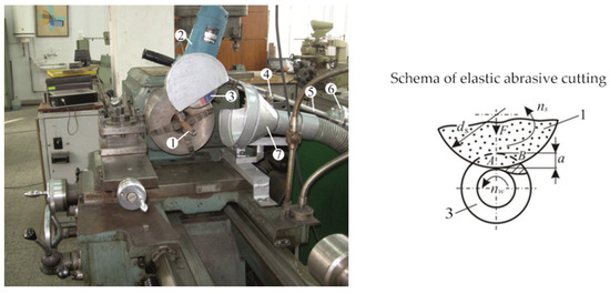
Figure 1.
Work device for elastic abrasive cutting: 1—workpiece; 2—angle grinder; 3—abrasive cut-off wheel; 4—bearing; 5—arm; 6—counterweight; 7—aspiration system.
The experimental investigations were carried out using a counter directional cutting method with cut-off wheels 41–180 × 22.2 × 3.0 A30RBF (EN 12413:2007) [9]. The material being machined had the shape of cylindrical rods with a diameter of dw = 30 mm made of steels C45 (1.0503) and 42Cr4 (1.7045) (BS EN 10277-2:2015) [49]—Table 1.

Table 1.
Chemical composition and physico-mechanical properties of steels being studied.
To construct the theoretical–experimental models for the production rate and manufacturing net cost of the elastic abrasive cutting of C45 and 42Cr4 steels—whose general form is given by Equation (12)—multifactorial experiments were conducted following an optimal central composite design with a number of trials N = 9. The levels of variation of the control factors are presented in Table 2 and ensure the operability of the cut-off wheels based on the following criteria: wear δ and time per cut tc as well as surface roughness Ra ≤ 2.5 µm and absence of thermal defects [3,39]. The cut-off wheel initial diameter and the diameter after the last cutting cycle are = 180 mm and = 120 mm.
Table 2.
Factor levels in design of experiments.
The values of the response variables Qw,r and Ct,r in each trial were determined in accordance with the analytical Relationships (1) and (2), as the number of working cycles mr and the average duration of the working cycle ts,r for elastic abrasive cutting of C45 and 42Cr4 steels were calculated using Relationships (6) and (11). The values of the coefficients a, b, p, and q (Table 3) were determined based on the empirical models for cut-off wheel wear and time per cut developed in [39], whose general forms are represented by Equations (4) and (8), respectively.
Table 3.
Coefficients in theoretical–experimental models (4) and (8) for wear and time per cut [38].
3.1.2. Results and Modelling
Table 4 includes the designs of the experiments with the values of the studied response variables of the elastic abrasive cutting process, and Table 5 includes the theoretical–experimental models for the production rate and manufacturing net cost of the elastic abrasive cutting of steels C45 and 42Cr4.
Table 4.
Design of experiments and response variables of elastic abrasive cutting.
Table 5.
Theoretical–experimental models for production rate and manufacturing net costs and statistic characteristics of models.
The constructed models include only the significant regression coefficients. They are adequate, as the condition is satisfied with a 95% confidence level, and describe with high accuracy the relationships between the studied response variables and the control factors ()—as shown in Table 5.
Figure 2 presents the influence of the cutting conditions on production rate and manufacturing net cost, according to the developed theoretical–experimental models (Table 5). Analysis of variance (ANOVA) was carried out using QStatLab to determine the degree of influence of the control factors on the studied response variables. The ANOVA interaction plots for the production rate and manufacturing net cost are shown in Figure 3.
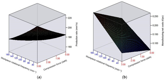
Figure 2.
Graphical visualization of models for elastic abrasive cutting of 42Cr4 steel: (a) production rate Qw2 and (b) manufacturing net cost Ct2.
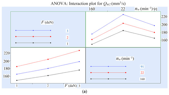
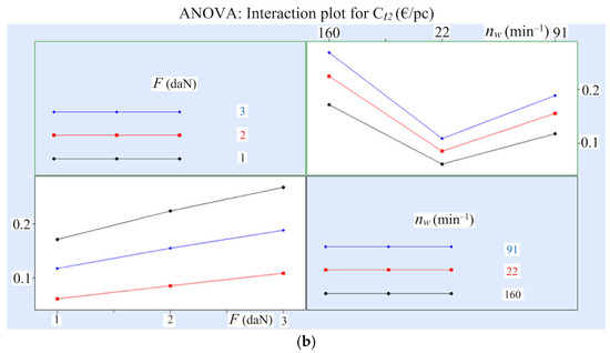
Figure 3.
Interaction plots for the response variables of the elastic abrasive cutting process of steel 42Cr4: (a) production rate Qw2 and (b) manufacturing net cost Ct2.
3.1.3. Analysis of the Experimental Results
The conducted study and modelling of the economic response variables of the elastic abrasive cutting of steels C45 and 42Cr4 show that they depend on both the workpiece rotational frequency nw and the compression force F. This is due to the significant influence of F and nw on the wear of the cut-off wheel and the time per cut, which have been theoretically and experimentally investigated in [39,45].
The analysis of the empirical models (Table 5) and the graphics plotted on the basis of them (Figure 2), as well as the interpretation of ANOVA results (Figure 3), make it possible to draw the following conclusions:
- An increase in the workpiece rotation frequency within the studied range leads to a corresponding rise in the manufacturing net cost (by 2.5 to 2.8 times) and a decrease in process production rate (by 15.9% to 18.8% for steel C45 and by 18.9% to 22.1% for steel 42Cr4), with the influence of nw becoming more pronounced as the compression force F decreases. The increase in manufacturing net cost and the reduction in production rate are associated with the intensified wear of the cut-off wheel and the increase in time per cut, resulting from the greater thickness of the material layer being cut by a single abrasive grain, which leads to increased loading on the abrasive grains and faster clogging of the cut-off wheel pores with chips [39,45], as well as the change in the ratio between the normal and tangential cutting forces, which reduces the cutting efficiency of the abrasive grains [50].
- An increase in the compression force leads, on the one hand, to a rise in the production rate (by 19.2% to 23.4% when processing steel C45 and by 17.3% to 22.2% when processing steel 42Cr4). On the other hand, it also results in an increase in manufacturing net cost (by 50.9% to 72.8% for steel C45 and by 55.2% to 74.3% for steel 42Cr4). This is associated with an increase in the length of the contact arc and the cutting depth [3,37,38,39], which leads to faster clogging of the cut-off wheel pores with chips and abrasive particles and a rise in temperature in the cutting zone. The influence of the compression force becomes more significant as the workpiece rotational frequency decreases.
- The cutting conditions under which the production rate of the elastic abrasive cutting process is maximum differ from those under which the manufacturing net cost is minimum. The maximum production rate is achieved at a compression force of daN and workpiece rotational frequency min−1 ( mm3/s—for steel C45; mm3/s—for steel 42Cr4), while the minimum manufacturing net cost is achieved at daN and min−1 for steel C45 ( EUR/pc) and daN и min−1 for steel 42Cr4 ( EUR/pc). In this context, it is of particular interest to determine the cutting conditions that provide the best combination of maximum production rate and minimum manufacturing net cost in elastic abrasive cutting. This would lead to an increase in the economic efficiency of the process.
3.2. Optimization of Elastic Abrasive Cutting Conditions
In accordance with the methodology presented in Section 2.3, a multi-objective compromise optimization was conducted to determine the optimal elastic abrasive cutting conditions (compression force and workpiece rotation frequency ), which ensure the best balance between maximum production rate and minimum manufacturing net cost. The concept of Pareto efficiency and the method of the generalized utility function were applied.
3.2.1. Multi-Objective Optimization Using the Concept of Pareto Efficiency
Pareto-optimal solutions were obtained (Table 6) for the values of the control factors (, ) of abrasive cutting for steels C45 and 42Cr4, under which the following conditions are satisfied:
where and are determined in accordance with the developed theoretical–experimental models for production rate and manufacturing net cost (Table 5).
Table 6.
Pareto-optimal solutions for elastic abrasive cutting conditions.
The optimal values of the compression force and the workpiece rotational frequency were determined by applying the NSGA-II genetic algorithm and software package QStatLab.
Under the predicted optimal conditions, confirmation run experiments were conducted to validate the results. In these experiments, the production rate and manufacturing net cost of the process were determined. The experimental values of the elastic abrasive cutting process response variables are presented in Table 6 and were calculated as the arithmetic mean of three observations for each combination (, ) of the control factors. A comparison between the experimental and the predicted values, according to the models (Table 4), of the elastic abrasive cutting process response variables (Table 5) shows that the maximum percentage error is 1.62% to 3.65% for the production rate and 3.38% to 3.59% for the manufacturing net costs. These results prove that the recommended elastic abrasive cutting conditions are optimum and correct.
3.2.2. Multi-Objective Optimization Using the Generalized Utility Function Method
- Modelling the generalized utility function
For the construction of the theoretical–experimental models of the geometric mean and arithmetic mean generalized utility functions (, ) with weight coefficients depending on the compression force F and the workpiece rotational frequency nw, whose general form was presented by Equation (15), the design of experiments theory was employed, and the software package QStatLab [46] was used.
Multifactor experiments were conducted according to an optimal central composite design with a number of trials N = 9 (Table 7). The values of the geometric mean generalized utility function for each trial were determined in accordance with Relationship (16). When calculating the values of the arithmetic mean generalized utility functions using Equation (17), the weight coefficients were set as follows: for ; ; for ; . In the first case, priority is given to ensuring a lower manufacturing net cost, while in the second case, priority is given to achieving a higher production rate. The utility coefficients and were determined using Formulas (18) and (19).
Table 7.
Design of experiment and generalized utility functions.
After statistical analysis of the experimental results (Table 7) using the method of regression analysis, theoretical–experimental models were obtained for the geometric mean () and arithmetic mean (, ) generalized utility functions with weight coefficients (Table 8). These models are considered adequate, as the condition is fulfilled with a 95% confidence level. The calculated and tabulated Fisher criterion values are presented in Table 8. The theoretical–experimental models describe with high accuracy the dependencies between the studied response variables and the control factors (determination coefficients , Table 8).
Table 8.
Theoretical–experimental models of generalized utility function and statistic characteristics of models.
Figure 4 graphically presents the effect of cutting conditions on the generalized utility functions according to the created theoretical–experimental models (Table 8).
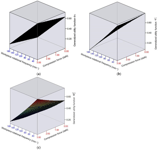
Figure 4.
Generalized utility functions in elastic abrasive cutting of 42Cr4 steel: (a) geometric mean generalized utility function; (b) arithmetic mean generalized utility function with weight coefficients w1 = 0.3 and w2 = 0.7; (c) arithmetic mean generalized utility function with weight coefficients w1 = 0.7 and w2 = 0.3.
To determine the influence of the control factors of the elastic abrasive cutting process on the generalized utility function, ANOVA was conducted. It was established that the cutting conditions exert different effects—both in nature and magnitude—on the generalized utility function, depending on the method used to determine the utility function and the type of material being machined.
The rotational frequency of the workpiece has the greatest influence. As nw decreases within the studied range, both the geometric mean and the arithmetic mean generalized utility functions with weight coefficients increase. The most significant change—approximately 9.8 times—is observed in the arithmetic mean utility function with weight coefficients w1 = 0.3 and w2 = 0.7 during elastic abrasive cutting of 42Cr4 steel at a compression force of the cut-off wheel against the workpiece daN.
An increase in the compression force leads, on one hand, to a rise (by up to 40%) in both the geometric mean and the arithmetic mean generalized utility function with weight coefficients w1 = 0.7 and w2 = 0.3 and, on the other hand, to a decrease in the arithmetic mean utility function with weight coefficients w1 = 0.3 и w2 = 0.7. The influence of the compression force on increases with the increase in the rotational frequency of the workpiece, with the most significant change observed at nw = 160 min−1 —by 82% for C45 steel and 4.2 times for 42Cr4 steel.
- Determination of the optimal conditions
By applying the methodology presented in Section 2.3.2, the optimal values of the control factors (compression force and rotational frequency of the workpiece ) for the elastic abrasive cutting process of C45 and 42Cr4 steels were determined. These optimal values satisfy one of the following conditions within the studied factor space (; ):
where , , and are determined in accordance with the developed models for the geometric mean () and arithmetic mean (, ) generalized utility functions with weight coefficients (Table 8). The problem was solved by searching for the Pareto-optimal solution using QstatLab and NSGA II (Figure 5). From the resulting Pareto front, the best compromise solutions (, ) were selected (Table 9).
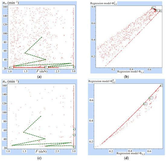
Figure 5.
Optimal conditions for the elastic abrasive cutting process of 42Cr4 steel: (a,b) and ; (c,d) and .
Table 9.
Optimum elastic abrasive cutting conditions determined by using the generalized utility function method.
To verify the predicted optimal conditions (, ), confirmation run experiments were conducted, during which the process production rate and manufacturing net cost were determined. A comparison between the experimental and the predicted values of response variables (Table 8), according to the models (Table 9), shows that the maximum percentage error is 0.19% for production rate and 1.76% for manufacturing net cost. These results prove that the recommended elastic abrasive cutting conditions are optimal and correct.
The analysis of the obtained results (Table 9) shows that the optimal conditions, when the priority is achieving maximum production rate, are as follows: compression force daN; workpiece rotational frequency of min−1 (the generalized objective functions and have maximum values). When the priority is achieving minimum manufacturing net cost, the optimal conditions are as follows: = 1 daN and min−1 (the generalized objective function has a maximum value).
The comparison of the production rate and manufacturing net cost of the elastic abrasive cutting process under the identified optimal conditions shows that when = 1 daN and min−1, the manufacturing net cost is 42–43% lower than that when daN, while the increase in production rate at higher compression force is only 18–19% lower. In this regard, it can be assumed that the best combination of maximum production rate and minimum manufacturing net cost is achieved during elastic abrasive cutting with a compression force = 1 daN and a workpiece rotational frequency min−1. These conditions ensure 10.7% higher production rate and 4.8% lower cost when cutting steel C45 compared to steel 42Cr4.
4. Conclusions
This article proposes a novel approach for the economic optimization of cutting conditions in the abrasive cutting process. The approach combines analytical and experimental modelling techniques and multi-objective optimization based on the NSGA-II genetic algorithm, aiming to increase production rate and minimize costs. It has been applied to the elastic abrasive cutting of two types of structural steels (medium-carbon steel C45 and alloyed chromium steel 42Cr4), yielding the following results:
- Theoretical–experimental models have been developed for the production rate and manufacturing net cost of the elastic abrasive cutting process, depending on the process control factors (compression force F and workpiece rotational frequency ). These models are based on original analytical expressions derived for the economic parameters of the abrasive cutting process, which take into account the durability of the cut-off wheel, estimated by the number of working cycles, and the time per cutting cycle. The models have been constructed using the design of experiments approach and the method of multifactor regression analysis.
- The significant influence of the operating conditions of the elastic abrasive cutting process on its economic parameters has been demonstrated. On one hand, increasing the rotational frequency of the workpiece within the studied range leads to an increase in manufacturing net cost (up to 2.8 times) and a decrease in process production rate (by up to 18.8% when cutting steel C45 and 22.1% when cutting steel 42Cr4). On the other hand, increasing the compression force results in a higher production rate of elastic abrasive cutting (by up to 23.4% when cutting steel C45 and by 22.2% when cutting steel 42Cr4), but it also significantly increases the manufacturing net cost (by up to 72.8% when cutting steel C45 and by 74.3% when cutting 42Cr4).
- It has been established that the cutting conditions under which the production rate is maximum are different from those under which the manufacturing net cost of the process is minimum. The maximum production rate is achieved at a compression force daN and a workpiece rotational frequency min−1 (for steels C45 and 42Cr4), while minimum manufacturing net cost is reached when daN and min−1 for steel C45 and when daN and min−1 for steel 42Cr4, respectively.
- To improve the economic efficiency of elastic abrasive cutting, a multi-objective compromise optimization has been conducted using two methods (determination of a compromise optimal region for the process conditions and the method of the generalized utility function). The optimal cutting conditions have been determined: compression force = 1 daN and min−1. These conditions ensure the best combination of maximum production rate and minimum manufacturing net cost, as follows: for steel C45, Qw = 204.9 mm3/s and Ct = 0.059 EUR/pc; for steel 42Cr4, Qw = 185.04 mm3/s and Ct = 0.062 EUR/pc, as well as surface roughness less than 2.5 µm and absence of thermal defects
The obtained theoretical and experimental results from the application of the new multi-objective economic optimization approach demonstrate that improving the economic efficiency of the abrasive cutting process is directly linked to selecting optimal operating conditions tailored to the specifics of the given process. These results provide opportunities for effective process control and can be successfully applied across all machine building companies.
Funding
This research was funded by the European Regional Development Fund within the OP “Research, Innovation and Digitalization Programme for Intelligent Transformation 2021–2027”, Project No. BG16RFPR002-1.014-0005 Center of competence “Smart Mechatronics, Eco- and Energy Saving Systems and Technologies”.
Institutional Review Board Statement
Not applicable.
Informed Consent Statement
Not applicable.
Data Availability Statement
Data are contained within the article.
Conflicts of Interest
The author declares no conflicts of interest.
References
- Neugebauer, R.; Hess, K.-U.; Gleich, S.; Pop, S. Reducing tool wear in abrasive cutting. Int. J. Mach. Tools Manuf. 2005, 45, 1120–1123. [Google Scholar] [CrossRef]
- Putz, M.; Cardonea, M.; Dix, M. Cut-off grinding of hardened steel wires-modelling of heat distribution. Proc. CIRP 2017, 58, 67–72. [Google Scholar] [CrossRef]
- Stoynova, A.; Aleksandrova, I.; Aleksandrov, A. Remote Nondestructive thermal control of elastic abrasive cutting. In Tri-Bology of Machine Elements-Fundamentals and Applications; Pintaude, G., Cousseau, T., Rudawska, A., Eds.; IntechOpen: London, UK, 2022. [Google Scholar] [CrossRef]
- Aleksandrova, I.; Hristov, H.; Ganev, G. Dynamic and technological characteristics of the process elastic abrasive cutting of rotating workpieces. J. Tech. Univ. Sofia Branch Plovdiv Fundam. Sci. Appl. 2011, 16, 123–128. [Google Scholar]
- Shaw, M. The Rating of Abrasive cutoff wheels. J. Eng. Ind. 1975, 97, 138–146. [Google Scholar] [CrossRef]
- Ganev, G. Elastic Abrasive Cutting of Rotational Workpieces in Mechanical Engineering. Ph.D. Thesis, Technical University of Gabrovo, Gabrovo, Bulgaria, 2013. [Google Scholar]
- Murata, R.; Shaw, M.C. The abrasive cut-off operation with oscillation. J. Eng. Ind. 1976, 98, 410–422. [Google Scholar] [CrossRef]
- ISO 8486-1; Bonded Abrasives—Determination and Designation of Grain Size Distribution. ISO: Geneva, Switzerland, 1996.
- Abrasive Tools and Materials, Disks for Cutting and Grinding. ZAI JSC-Bulgaria. Available online: https://zai-bg.com/en/ (accessed on 29 May 2025).
- Putz, M.; Cardone, M.; Dix, M.; Wertheim, R. Analysis of workpiece thermal behaviour in cut-off grinding of high-strength steel bars to control quality and efficiency. CIRP Ann. 2019, 68, 325–328. [Google Scholar] [CrossRef]
- Malkin, S.; Guo, C. Thermal analysis of grinding. CIRP Ann. 2007, 56, 760–782. [Google Scholar] [CrossRef]
- Wang, Z.; Li, Y.; Yu, T.; Zhao, J.; Wen, P.H. Prediction of 3D grinding temperature field based on meshless method considering infinite element. Int. J. Adv. Manuf. Technol. 2018, 100, 3067–3084. [Google Scholar] [CrossRef]
- Vologin, K. Selection of Rational Conditions for Cutting Workpieces of Difficult to Machine Material with Abrasive Wheels. Ph.D. Thesis, Moscow State University of Technology Stankin, Moscow, Russia, 2002. [Google Scholar]
- Li, J.; Liu, J. Numerical simulation of abrasive cutoff operation based on ALE adaptive meshing technique. AIP Adv. 2023, 13, 115033. [Google Scholar] [CrossRef]
- Eshghy, S. Thermal aspects of the abrasive cut off operation. Part 2-Tartition functions and optimum cut off. J. Eng. Ind. 1968, 90, 360–364. [Google Scholar] [CrossRef]
- Hou, H.; Komanduri, R. On the mechanics of the grinding process, Part III-Thermal analysis of the abrasive cutoff operation. Int. J. Mach. Tools Manuf. 2004, 44, 271–289. [Google Scholar] [CrossRef]
- Lopes, J.C.; Ribeiro, F.S.F.; Javaroni, R.L.; Garcia, M.V.; Ventura, C.E.H.; Scalon, V.L.; de Angelo Sanchez, L.E.; de Mello, H.J.; Aguiar, P.R.; Bianchi, E.C. Mechanical and thermal effects of abrasive cutoff applied in low and medium carbon steels using aluminum oxide cut-off wheel. Int. J. Adv. Manuf. Technol. 2020, 109, 1319–1331. [Google Scholar] [CrossRef]
- Luo, S.Y.; Tsai, Y.Y.; Chen, C.H. Studies on cut-off grinding of BK7 optical glass using thin diamond wheels. J. Mater. Process. Technol. 2006, 173, 321–329. [Google Scholar] [CrossRef]
- Levchenko, E.; Pokintelitsa, N. Investigation of thermal processes in abrasive pipe sampling. MATEC Web Conf. 2017, 129, 01082. [Google Scholar] [CrossRef][Green Version]
- Sahu, P.; Sagar, R. Development of abrasive cut-off wheel having side grooves. Int. J. Adv. Manuf. Technol. 2006, 31, 37–40. [Google Scholar] [CrossRef]
- Ni, J.; Yang, Y.; Wu, C. Assessment of water-based fluids with additives in grinding disc cutting process. J. Clean. Prod. 2019, 212, 593–601. [Google Scholar] [CrossRef]
- Ojolo, S.; Orisaleye, J.; Adelaja, A. Development of a high speed abrasive cutting machine. J. Eng. Res. 2010, 15, 1–8. [Google Scholar]
- Yoshida, T.; Nagasaka, K.; Kita, Y.; Hashimoto, F. Identification of a grinding wheel wear equation of the abrasive cut-off by the modified GMDH. Int. J. Mach. Tool Des. Res. 1986, 26, 283–292. [Google Scholar] [CrossRef]
- Yamasaka, M.; Fujisawa, M.; Oku, T.; Masuda, M.; Okamura, K. Improvement of straightness in precision cut-off grinding using thin diamond wheels. CIRP Ann. Manuf. Technol. 1990, 39, 333–336. [Google Scholar] [CrossRef]
- Awan, M.R.; Rojas, H.A.G.; Benavides, J.I.P.; Hameed, S. Experimental technique to analyze the influence of cutting conditions on specific energy consumption during abrasive metal cutting with thin discs. Adv. Manuf. 2022, 10, 260–271. [Google Scholar] [CrossRef]
- Awan, M.R.; Rojas, H.A.G.; Hameed, S.; Riaz, F.; Hamid, S.; Hussain, A. Machine learning-based prediction of specific energy consumption for cut-off grinding. Sensors 2022, 22, 7152. [Google Scholar] [CrossRef]
- Awan, M.R.; Rojas, H.A.G.; Benavides, J.I.P.; Hameed, S.; Hussain, A.; Egea, A.J.S. Specific energy modeling of abrasive cut off operation based on sliding, plowing, and cutting. J. Mater. Res. Technol. 2022, 18, 3302–3310. [Google Scholar] [CrossRef]
- Ortega, N.; Martynenko, V.; Perez, D.; Krahmer, D.M.; López de Lacalle, L.N.; Ukar, E. Abrasive disc performance in dry-cutting of medium-carbon steel. Metals 2020, 10, 538. [Google Scholar] [CrossRef]
- Ortega, N.; Bravo, H.; Pombo, I.; Sánchez, J.; Vidal, G. Thermal analysis of creep feed grinding. Procedia Eng. 2015, 132, 1061–1068. [Google Scholar] [CrossRef]
- Braz, C.O.; Ventura, C.E.H.; de Oliveira, M.C.B.; Antonialli, A.H.S.; Ishikawa, T. Investigating the application of customized abrasive cutoff wheels with respect to tool wear and subsurface integrity in metallographic cutting of pure titanium. Metallogr. Microstruct. Anal. 2019, 8, 826–832. [Google Scholar] [CrossRef]
- Riga, A.; Scott, C. Failure analysis of an abrasive cut-off wheel. Eng. Failure Anal. 2001, 8, 237–243. [Google Scholar] [CrossRef]
- Galinovskii, A.; Martysyuk, D.A.; Katkova, E.D.; Muzafarova, A.D.; Mikhailov, A.A. Developing a method of estimating the efficiency of cutting with abrasive cutoff wheels. Polym. Sci. Ser. 2024, 17, 934–940. [Google Scholar] [CrossRef]
- Nagasaka, K.; Yoshida, T.; Kita, Y.; Hashimoto, F. Optimum combination of operating parameters in abrasive cut-off. Int. J. Mach. Tool Manuf. 1987, 27, 167–179. [Google Scholar] [CrossRef]
- Farmer, D.A.; Shaw, M.C. Economics of the abrasive cutoff operation. J. Eng. Ind. 1967, 89, 514–518. [Google Scholar] [CrossRef]
- Kaczmarek, J. The effect of abrasive cutting on the temperature of grinding wheel and its relative efficiency. Arch. Civ. Mech. Eng. 2008, 8, 81–91. [Google Scholar] [CrossRef]
- Kaczmarek, J. Using a thermovision method for measuring temperatures of a workpiece during abrasive cut-off operation. Adv. Manuf. Sci. Technol. 2011, 35, 85–95. Available online: https://scispace.com/pdf/application-of-neural-networks-to-control-of-drive-functions-1o0lwnyiqk.pdf (accessed on 31 May 2025).
- Stoynova, A.; Aleksandrova, I.; Aleksandrov, A.; Goranov, G. Non-contact measurement and monitoring of cut-off wheel wear. In Proceedings of the 28th International Scientific Conference Electronics, Sozopol, Bulgaria, 12–14 September 2019. [Google Scholar] [CrossRef]
- Stoynova, A.; Aleksandrova, I.; Aleksandrov, A.; Ganev, G. Infrared thermography for elastic abrasive cutting process monitoring. MATEC Web Conf. 2018, 210, 02018. [Google Scholar] [CrossRef]
- Aleksandrova, I.; Stoynova, A.; Aleksandrov, A. Modelling and multi-objective optimization of elastic abrasive cutting of C45 and 42Cr4 steels. J. Mech. Eng./Stroj. Vestn. 2021, 67, 635–648. [Google Scholar] [CrossRef]
- Khalilpourazari, S.; Khalilpourazary, S. Optimization of time, cost and surface roughness in grinding process using a robust multi-objective dragonfly algorithm. Neural Comput. Appl. 2020, 32, 3987–3998. [Google Scholar] [CrossRef]
- Tran, T.-H.; Luu, A.-T.; Nguyen, Q.-T.; Le, H.-K.; Nguyen, A.-T.; Hoang, T.-D.; Le, X.-H.; Banh, T.-L.; Vu, N.-P. Optimization of replaced grinding wheel diameter for surface grinding based on a cost analysis. Metals 2019, 9, 448. [Google Scholar] [CrossRef]
- Tran, T.-H.; Hoang, X.-T.; Le, H.-K.; Nguyen, Q.-T.; Nguyen, T.-T.; Nguyen, T.-T.-N.; Jun, G.; Vu, N.-P. A study on cost optimization of external cylindrical grinding. Mater. Sci. Forum 2020, 977, 18–26. [Google Scholar] [CrossRef]
- Dzebo, S.; Morehouse, J.B.; Melkote, S.N. A methodology for economic optimization of process parameters in centerless grinding. Mach. Sci. Technol. 2012, 6, 355–379. [Google Scholar] [CrossRef]
- Jiang, W.; Lv, L.; Xiao, Y.; Fu, X.; Deng, Z.; Yue, W. A multi-objective modeling and optimization method for high efficiency, low energy, and economy. Int. J. Adv. Manuf. Technol. 2023, 128, 2483–2498. [Google Scholar] [CrossRef]
- Aleksandrova, I.; Ganev, G.; Hristov, H. Performance of cut-off wheels during elastic abrasive cutting of rotating workpieces. Teh. Vjesn. 2019, 26, 577–583. [Google Scholar] [CrossRef]
- Vuchkov, I.N.; Vuchkov, I.I. QStatLab Professional, version 6.1.1.3; Statistical Quality Control Software, User’s Manual; QStatLab: Sofia, Bulgaria, 2009.
- Mukherjee, I.; Ray, P. A review of optimization techniques in metal cutting processes. Comput. Ind. Eng. 2006, 50, 15–34. [Google Scholar] [CrossRef]
- Stoyanov, S. Optimization of Manufacturing Processes; Tehnika: Sofia, Bulgaria, 1993. [Google Scholar]
- Steel and Cast Iron Standards; EN 10277: Steel grades/numbers. Available online: http://www.steelnumber.com/en/standard_steel_eu.php?gost_number=10277 (accessed on 30 May 2025).
- Aleksandrova, I.; Ganev, G.; Hristov, H. Compression forces and power during elastic abrasive cutting of rotating workpieces. Teh. Vjesn. 2016, 23, 343–348. [Google Scholar] [CrossRef]


Disclaimer/Publisher’s Note: The statements, opinions and data contained in all publications are solely those of the individual author(s) and contributor(s) and not of MDPI and/or the editor(s). MDPI and/or the editor(s) disclaim responsibility for any injury to people or property resulting from any ideas, methods, instructions or products referred to in the content. |
© 2025 by the author. Licensee MDPI, Basel, Switzerland. This article is an open access article distributed under the terms and conditions of the Creative Commons Attribution (CC BY) license (https://creativecommons.org/licenses/by/4.0/).