Article

Double Wishbone Suspension: A Computational Framework for Parametric 3D Kinematic Modeling and Simulation Using Mathematica

1
Department of Computer Science and Engineering, University of Bologna, 40126 Bologna, Italy
2
Rosen Center for Advanced Computing, Purdue University, West Lafayette, IN 47907, USA
*
Authors to whom correspondence should be addressed.
Technologies 2025, 13(8), 332; https://doi.org/10.3390/technologies13080332 (registering DOI)
Submission received: 1 June 2025 / Revised: 15 July 2025 / Accepted: 28 July 2025 / Published: 1 August 2025
(This article belongs to the Section Manufacturing Technology)

Abstract

The double wishbone suspension (DWS) system is widely used in automotive engineering because of its favorable kinematic properties, which affect vehicle dynamics, handling, and ride comfort; hence, it is important to have an accurate 3D model, simulation, and analysis of the system in order to optimize its design. This requires efficient computational tools for parametric study. The development of effective computational tools that support parametric exploration stands as an essential requirement. Our research demonstrates a complete Wolfram Mathematica system that creates parametric 3D kinematic models and conducts simulations, performs analyses, and generates interactive visualizations of DWS systems. The system uses homogeneous transformation matrices to establish the spatial relationships between components relative to a global coordinate system. The symbolic geometric parameters allow designers to perform flexible design exploration and the kinematic constraints create an algebraic equation system. The numerical solution function NSolve computes linkage positions from input data, which enables fast evaluation of different design parameters. The integrated 3D visualization module based on Mathematica’s manipulate function enables users to see immediate results of geometric configurations and parameter effects while calculating exact 3D coordinates. The resulting robust, systematic, and flexible computational environment integrates parametric 3D design, kinematic simulation, analysis, and dynamic visualization for DWS, serving as a valuable and efficient tool for engineers during the design, development, assessment, and optimization phases of these complex automotive systems.

1. Introduction

The design and behavior of suspension systems determine how well ground vehicles perform while ensuring safety and delivering comfortable rides [1]. The systems control how vehicle bodies interact with road surfaces, thus affecting vehicle handling dynamics and stability and passenger comfort. The double wishbone suspension (DWS), known as short-long arm (SLA) suspension (shown in Figure 1), has become a standard choice for performance and racing vehicles as well as heavy-duty applications [2,3]. Engineers choose this system because its beneficial kinematic properties enable them to adjust camber change, roll center height, scrub radius throughout wheel travel, and body roll movements to maximize tire grip and vehicle handling capabilities [4,5].
A DWS system’s kinematic behavior depends on its three-dimensional (3D) geometry, which consists of control arm lengths (wishbones) and their chassis mounting points (hardpoints) and steering linkage geometry [6]. The geometric parameters that differ slightly from standard values produce major changes in wheel orientation and body position, which affects essential performance metrics. The automotive design process requires precise 3D kinematic modeling and simulation tools to evaluate suspension performance, compare design alternatives, and optimize geometry before physical prototyping becomes necessary [7].
Figure 1. Three-dimensional visualization of a double wishbone suspension system detailing the layout of control arms, connection points, and wheel assembly [8].
Technologies 13 00332 g001
The optimization of DWS geometry requires examination of a broad design space that contains multiple geometric parameters [9]. The analysis demands computational tools that both deliver precise kinematic simulation and enable fast parametric studies [6]. Engineers require tools that enable fast modification of input parameters such as hard-point coordinates and link lengths while showing the resulting kinematic changes. The designers require effective visualization tools to understand the spatial motion of multiple links in DWS mechanisms because these tools help them identify interference and undesirable kinematic characteristics [10].
While several methods and software tools exist for suspension analysis, they present a trade-off between power and accessibility. Industry-standard multibody dynamics (MBD) packages like Adams and Simpack offer high-fidelity simulation, but their utility for rapid design exploration is often hampered by significant licensing costs, steep learning curves, and operational complexity [11,12]. This complexity can create a barrier during the early, iterative stages of design or in academic research where agility and intuitive parametric adjustment are paramount. On the other hand, purely analytical methods such as vector loop and screw theory, while insightful, quickly become mathematically intractable when applied to complex 3D spatial mechanisms with multiple parametric variations [13]. To bridge this gap, our research introduces a framework that directly confronts these limitations of complexity and cost. Using Wolfram Mathematica, we present a solution that unites the precision of mathematical modeling with the flexibility of symbolic computation and the immediacy of interactive visualization. This approach lowers the barrier to entry, allowing engineers to perform efficient and intuitive parametric studies without the overhead associated with traditional MBD software [14].
This study presents a computational framework in Wolfram Mathematica for parametric 3D kinematic modeling and simulation and interactive visualization of double wishbone suspension systems to meet this need. The framework uses homogeneous transformation matrices for spatial precision and Mathematica’s symbolic and numerical capabilities to create a robust, accessible tool for engineers and researchers. The framework enables engineers to perform parametric geometry definition and automated kinematic constraint equation generation and solution while providing dynamic 3D visualization to efficiently analyze DWS designs.
The rest of this paper is organized as follows. Section 2 reviews prior literature on suspension modeling to contextualize our contribution. Section 3 details the core mathematical methodology, explaining the use of coordinate transformations and homogeneous matrices to define the geometry of the suspension. Following this, Section 4 describes the formulation of the kinematic constraint equations that govern the mechanical links and the challenges to solving them. The framework for rendering the 3D model is presented in Section 5. Section 6 introduces the dynamic kinematic solver, discusses its performance and complexity, and demonstrates its utility for interactive analysis. Finally, Section 7 provides concluding remarks and suggests directions for future research.

2. Related Work

The double wishbone suspension (DWS) remains an active area of research in automotive engineering because of its favorable kinematic performance and the increasing need for more refined optimization tools. Recent works address a number of complementary challenges, including simplified analytical models, multi-body simulations with flexible components, and integrated methods for geometric optimization and real-time visualization.
Although early approaches relied on basic two-dimensional planar models, the need to precisely predict wheel alignment parameters such as camber, caster, and toe drove the adoption of more advanced 3D parametric modeling. For instance, some forward kinematics approaches used screw theory to achieve high accuracy but offered limited interactive functionality [15]. A matrix-based system was also used to analyze bump-steer effects while focusing on real-time simulation for motorsport applications [6]. A comprehensive 3D multi-body dynamic (MBD) model was created to study the linked suspension effects [3,16]. In [3], the authors explained how rubber bush stiffness affects both the static alignment and transient responses of the system. MBD software tools such as Adams and Simpack deliver powerful functionality, but their use for symbolic or parametric analysis becomes complicated because users need to write complex scripts and perform multiple iterations [12,17].
The field of vehicle suspension geometry research has increasingly turned to symbolic computation to embed adjustable parameters for real-time design exploration [15], previous work has focused on developing closed-loop constraint equations for SLA suspensions [6] and creating reconfigurable prototypes without the need to rewrite code for new layouts [3,10]. Crucially, the validation of these models typically relies on benchmarking their kinematic outputs against results from established MBD software like Adams or comparing them to measurements from physical test rigs. Although this quantitative validation is the gold standard for verifying final designs, it is often performed as a discrete, final step after the design has been established.
Our framework complements these traditional validation methods by introducing a form of continuous, interactive visual validation. Rather than waiting for a post-simulation data comparison, our approach provides immediate graphical feedback on the physical plausibility of the suspension geometry as parameters are adjusted. The dynamic solver in Figure 1 instantly confirms whether a given set of parameters yields a solvable, physically coherent linkage. This prioritizes configurational correctness throughout the design process, ensuring that engineers do not spend time on designs that are geometrically invalid. In this way, our tool serves as a powerful front-end for rapid iteration, allowing designers to confidently explore a wide design space before committing a smaller set of valid designs to more rigorous (and time-consuming) quantitative benchmarking.
Advanced computational tools, particularly Wolfram Mathematica, have shown advantages in solving both symbolic and numeric problems [18]. The real-time parameter manipulation through built-in “Manipulate” and symbolic constraint solution within this system creates a more interactive design environment than typical multi-body codes, which operate through scripting [19]. This method reduces the time needed to evaluate camber-toe sensitivity when testing various geometric modifications.
The study in Table 1 demonstrate the capability of symbolic computation for suspension kinematics, but they mainly concentrate on either numerical performance or static geometry exploration. Real-time symbolic geometry solvers with interactive visualization, as presented in this paper, remain rare and underrepresented.
Table 1. Overview of symbolic modeling approaches for suspension systems.
System TypeSymbolic MethodFocus AreaVisualizationInteractivity
General suspensions [20]Mixed Symbolic-NumericalK&C modeling
Double wishbone [21]Block-triangularizationReal-time dynamics✓ (simulator)Partial
Generic link suspensions [22]Symbolic sensitivity analysisDesign optimization
McPherson [23]Mathematica-based symbolic kinematicsStatic geometry
Double wishbone [24]Coupled kineto-dynamicsPerformance trade-offs
Double wishboneFull symbolic + numerical solvingReal-time kinematics & visualization✓ (3D interactive)✓ (live parametric solver)

3. Methodology

The section describes a complete symbolic modeling approach to the geometric analysis and visualization of a double wishbone suspension system shown in Figure 2. The method is based on multibody kinematics and uses homogeneous transformation matrices to define the spatial relationships between suspension components. The system is modeled in Wolfram Mathematica, using symbolic computation to derive position vectors, enforce geometric constraints, and solve for unknown joint configurations under varying parameters.

3.1. Coordinate Transformation

3.1.1. Rotation Matrix

The development of three-dimensional models of geometry and kinematics represents the essential base for simulating double wishbone suspension system behavior. A core assumption of our kinematic model is that all suspension components including the control arms, upright, and linkages are treated as ideal rigid bodies. This means that any deflection, bending, or elastic deformation of the components under load is considered negligible for this analysis. This rigid-body assumption allows us to accurately model the system’s motion pathways and geometric relationships. The initial step requires establishing spatial relationships and movement capabilities for all suspension assembly components. The spatial transformations of components are made possible by rotation matrices, which operate on the principal axes ( X , Y , Z ) . The mathematical building blocks known as matrices enable us to model suspension system articulations during wheel travel and steering input and chassis dynamics responses. This establishes rotation operations in symbolic and modular form for modeling purposes.
In 3D mechanics, a rigid body’s orientation can be described by applying successive rotations about coordinate axes. These rotations are typically represented by orthogonal matrices. Here, we define three such matrices:
  • Rotation about the X-axis (pitch)
    rotX ( α ) = 1 0 0 0 cos ( α ) sin ( α ) 0 sin ( α ) cos ( α )
    This rotates a point or vector around the X-axis by an angle α . It is used, for instance, to simulate the upper control arm’s pitch motion relative to chassis mounting points.
  • Rotation about the Y-axis (yaw)
    rotY ( β ) = cos ( β ) 0 sin ( β ) 0 1 0 sin ( β ) 0 cos ( β )
    This rotation is essential to simulate how the wheel steers around a vertical axis, such as when a vehicle turns left or right.
  • Rotation about the Z-axis (roll)
    rotZ ( γ ) = cos ( γ ) sin ( γ ) 0 sin ( γ ) cos ( γ ) 0 0 0 1
    This represents rotation about the Z-axis, often used in modeling chassis roll or wheel tilt caused by lateral forces.
This contains separate functions that take an angle as input to generate 3 × 3 rotation matrices. The matrices function as input with coordinate vectors of suspension points or serve as inputs to create compound transformations r o t Z [ γ ] . r o t Y [ β ] . r o t X [ α ] to simulate complex motions. The matrices serve an essential purpose because they enable the simulation to rotate points on the suspension, like upright pivots, to replicate actual movement. The rotation matrices will serve an essential purpose in our model by determining the position and orientation of moving components, including the upper and lower wishbones and steering knuckle, throughout wheel travel and body roll.

3.1.2. Combine 3D Rotation

Each matrix rotates the coordinate frame around its respective axis, and they are combined in specific orders to reflect the actual mounting orientation of the suspension parts. Multiple axis rotations are combined using matrix multiplication. Two rotation orders are used:
  • XYZ Order: Common for the lower control arm and other base-mounted parts.
  • ZXY Order: Used for parts like the upper control arm where the rotation hierarchy differs.
These are calculated as follows:
rot 3 D ( α , β , γ ) = rotZ ( γ ) · rotY ( β ) · rotX ( α )
rot 3 DZXY ( α , β , γ ) = rotZ ( γ ) · rotX ( α ) · rotY ( β )
This step is critical in ensuring the spatial alignment of the components matches the physical reality of how parts are assembled in an actual suspension system. Multiple angular transformations applied in sequence produce their cumulative effect, which the composite rotation functions encapsulate. The double wishbone suspension uses these functions to determine the end spatial orientation of components that experience motions simultaneously during cornering and vertical travel. The ability to use different rotation orders between Z Y X and Z X Y provides valuable modeling versatility, which ensures compatibility with various suspension layouts and coordinate systems. The functions establish a basis for exact and flexible dynamic behavior simulation of the suspension assembly.

3.2. Homogeneous Transformation

The ability to rotate components in space needs translation capabilities to move components between different positions. The double wishbone suspension requires this functionality because its control arms and wheel hub need to perform both rotation and 3D translation motions when the suspension compresses or extends. The homogeneous transformation matrix unifies rotation and translation into a single mathematical operation. The formulation provides a unified matrix representation of rigid-body transformation, which includes both orientation and position changes for efficient point transformation calculations and motion chaining between multiple components.
The homogeneous transformation matrix is a 4 × 4 matrix that combines a 3D rotation and translation into a single structure. This is critical for transforming points or frames in 3D space in robotics, vehicle kinematics, and mechanical simulation.
rot: a 3 × 3 rotation matrix (like rot3D).
trans: a 3 × 1 column vector representing translation.
The resulting homogeneous transformation matrix is
T = r 11 r 12 r 13 t x r 21 r 22 r 23 t y r 31 r 32 r 33 t z 0 0 0 1
We use ArrayFlatten to assemble this structure by nesting the following submatrices:
  • Top-left block: the rotation matrix rot
  • Top-right block: the translation vector trans
  • Bottom row: a row vector [ 0 0 0 1 ]
This matrix allows to perform rigid-body transformations by multiplying it with a homogeneous point vector:
x y z 1
effectively applying both rotation and translation in one step.
The homogeneous transformation matrix provides a unified form to encapsulate both orientation and position, which makes it essential for simulating the complete spatial motion of mechanical components. The double wishbone suspension model employs this matrix to transmit chassis movements that result in wheel hub motion. The system enables exact position and direction calculations following multiple transformations, which supports both visualization and numerical analysis. The model gains the ability to measure geometric results such as camber angle and kingpin inclination and virtual swing arm trajectories through this formulation.

3.2.1. Numerical Considerations and Stability

Although the use of chained matrix multiplications is a powerful and standard technique in kinematics, it is pertinent to address the potential for numerical inaccuracies. In computational mechanics, sequential matrix operations can lead to the accumulation of floating-point rounding errors, potentially affecting the precision of the final calculated positions.
However, several factors in our proposed framework mitigate this issue. First, our model is solved for discrete static equilibrium configurations using NSolve, rather than through a time-stepping dynamic simulation where errors would compound iteratively over a long duration. Second, the framework is implemented in Wolfram Mathematica, which utilizes an arbitrary-precision arithmetic engine. This allows the solver to maintain a high degree of numerical precision throughout its calculations, minimizing the impact of rounding errors that might be more significant in standard double-precision environments. For the scale of the system being analyzed a single suspension corner with a limited number of interconnected bodies these factors ensure that the numerical accuracy is more than sufficient and that the stability of the matrix operations does not adversely affect the validity of the kinematic solutions.

3.2.2. Transformations from Chassis Frame to Upper and Lower Control Arm

This step describes how the upper and lower control arms are mounted and oriented relative to the chassis coordinate system with the rotation and transformation frameworks in place. In a real-world double wishbone suspension, these control arms form the foundation of the suspension triangle and dictate the upright’s motion path. We can simulate their relative positions, orientations, and behavior as independent yet connected subsystems by defining transformations from the chassis frame to the UCA and LCA frames. It uses the previously defined composite rotation and homogeneous transformation functions to express this relationship parametrically.
These two functions define rigid-body transformations from the chassis coordinate system to the upper control arm (UCA) and lower control arm (LCA) coordinate systems. Each function takes six inputs: Euler angles ( α , β , γ ), defining the control arm’s orientation and the translational offsets ( t x , t y , t z ) defining the control arm’s mounting position on the chassis.
  • ACUCA[ α , β , γ , t x , t y , t z ]: This constructs the transformation matrix for the upper control arm using the Z-X-Y (rot3DZXY) rotation sequence. This choice reflects a mounting configuration where roll (Z), camber/caster tilt (X), and toe or fore-aft direction (Y) are sequentially applied. This is often relevant to higher control arms whose mounts might be angled or non-orthogonal to the main chassis frame. The function returns a 4 × 4 matrix representing the full pose (position and orientation) of the UCA frame in the chassis coordinate system.
  • ACLCA[ α , β , γ , t x , t y , t z ]: This defines the lower control arm transformation, using the Z-Y-X (rot3D) rotation sequence. This is a standard Euler sequence for typical orthogonal setups, where the LCA is mounted more parallel to the chassis axes. Likewise, it returns a homogeneous transformation matrix.
In both cases, the translation vector is structured as a 3 × 1 column vector:
trans = t x t y t z
The result is a homogeneous transformation that can now be used to position and orient suspension elements relative to these control arms, such as link pivot points, the upright, or spring/damper connections.

3.2.3. Transformations from UCA and LCA Frames to Upright Frame

The control arms now have their positions defined relative to the chassis, so the next step in suspension modeling deals with the upright, which serves as the rigid link between the wheel hub and the upper and lower control arms. The upright’s motion path depends on its connections to control arms and sometimes additional linkages, including tie rods or pushrods. The model uses transformation matrices to describe how the upright relates in terms of position and orientation to both the upper and lower control arms. The realistic upright articulation simulation depends on these transformations, which also determine the wheel motion simulation. There is a distinct transformation for the connecting rod, allowing the model to represent steering links and load-transmitting members.
  • AUCUpright[ α , β , γ , t x , t y , t z ]: This models the upper control arm to upright transformation. The transformation employs the Z-X-Y rotation order (rot3DZXY), which works best for systems that rotate first around the Z-axis, then translate along the X-axis, and finally rotate around the Y-axis. The matrix is composed with a translation vector ( t x , t y , t z ) , which specifies the physical mounting position of the upright relative to the UCA.
  • ALCUpright[ α , β , γ , t x , t y , t z ]: This transformation connects the lower control arm to the upright. It follows the Z-Y-X Euler sequence (rot3D), which is suitable for most mounting configurations where the upright moves vertically with LCA travel while also rotating due to steering input.
  • ACRod[ β , γ , t x , t y , t z ]: This transformation defines a rod or link, likely used as a tie rod or pushrod. The rotation is limited to the Y and Z axes, as given by rot3D[0, β , γ ], indicating that the rod pivots only in the yaw and roll directions. This reflects typical tie rod behavior—steering left and right while allowing vertical compliance. Again, the translation vector ( t x , t y , t z ) defines the position of this rod base relative to the chassis frame or another reference component.
This model defines transformation matrices from control arms and connecting rods to the upright to establish a clear modular pathway for simulating upright behavior under suspension articulation. These functions encode both the geometry and orientation of the links, ensuring that the upright responds correctly to the control arm movement and steering input. Separate rod transformation enables steering dynamics or force transmission through tie rods or actuators. The collective transformations create a fully constrained spatial framework for the upright which enables realistic wheel movement and suspension kinematics and structural and dynamic system interactions.

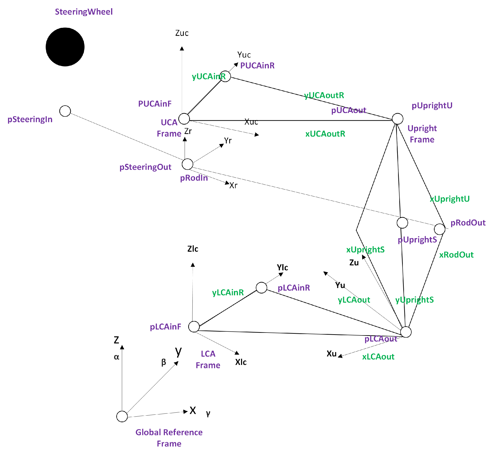
3.3. Local Frame Point

Any multibody mechanical system requires the definition of essential geometric points that represent the mounting and connection interfaces between components, especially in spatial mechanisms such as the double wishbone suspension. The system includes inboard and outboard pivots of control arms together with upright connection points and link attachment points for rods and dampers. The points exist initially within their specific component local coordinate frames. The points become compatible with transformation matrices through homogeneous coordinates (with a fourth coordinate of 1) for accurate mapping between the global (chassis) frame and intermediate frames. The following code establishes such points parametrically to enable complete suspension kinematic assembly.
Homogeneous points—vectors in 4D in the following form:
x , y , z , 1
The 4 × 4 transformation matrices we built before become directly compatible with the homogeneous points [ x , y , z , 1 ] .
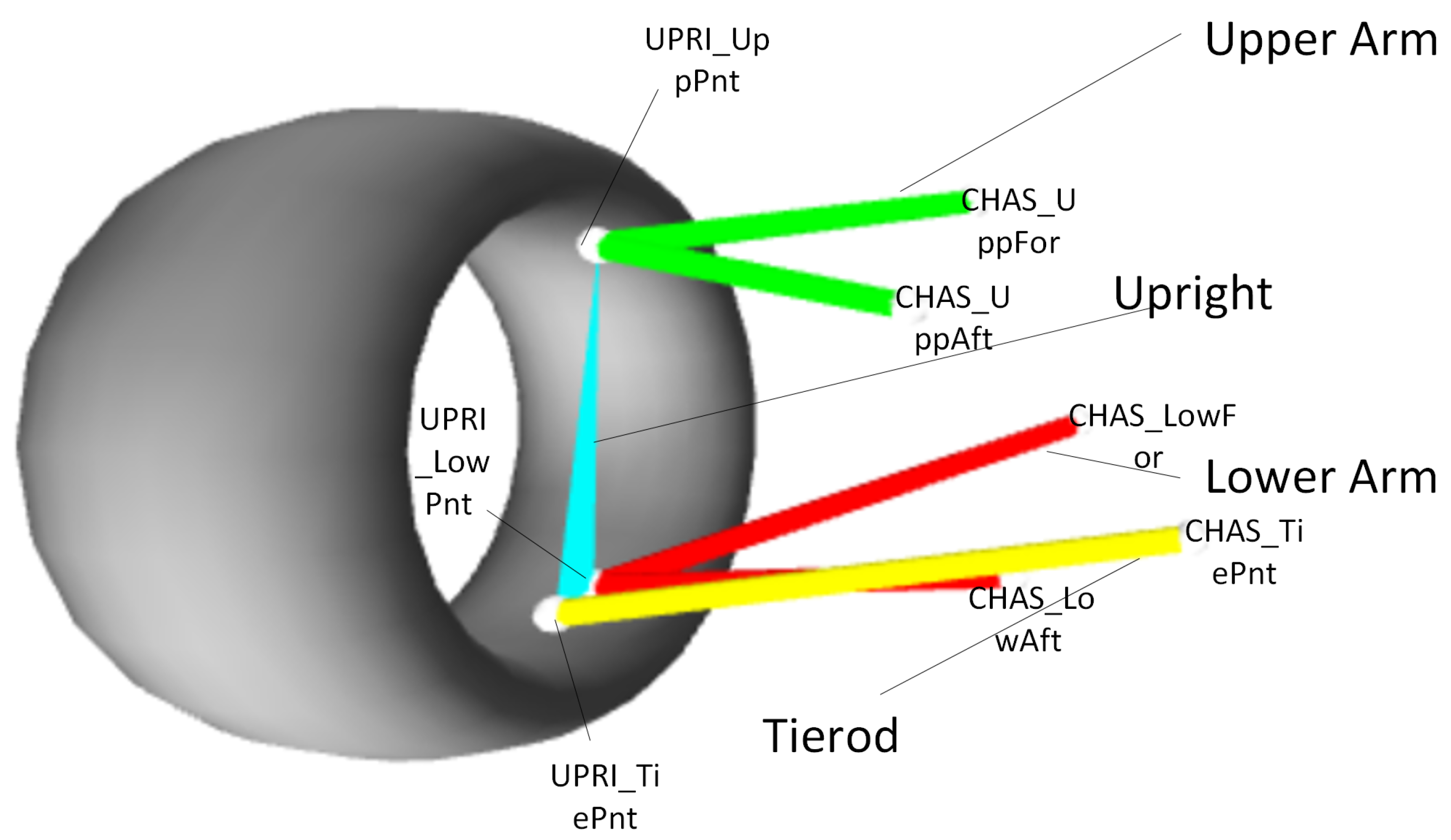
  • Upper Control Arm (UCA): pUCAinF[] is the inboard (frame) mounting point of the UCA—typically attached to the chassis. pUCAinR[yUCAinR] is a parameterized inboard mounting on a rail, offset in the Y-axis. The parameter allows users to model various mount points. pUCAout[xUCAout, yUCAout] is the outer (upright) connection point of the UCA in its local frame.
  • Tie Rod or Pushrod: pRodin[]: The base point of the rod in its frame (likely attached to the steering rack or chassis). pRodout[xRodout]: The upright-end attachment point of the rod, parameterized by X—commonly used in steering simulations.
  • Upright: pUprightU[xUprightU] is the upper pivot point where the UCA connects to the upright. pUprightL[] is the lower pivot point of the upright, often aligned as the origin in its local frame. pUprightS[xUprightS, yUprightS] is a side point on the upright—likely for the tie rod or shock mount.
  • Lower Control Arm (LCA): pLCAinF[] is the inboard (frame) mounting of the LCA. pLCAinR[yLCAinR] is another inboard option along the Y-axis. pLCAout[xLCAout, yLCAout] is the outer joint where the LCA connects to the upright.
These points operate as plug-and-play components because we specify the configuration through parameters (like xUCAout or yLCAinR) before applying transformation matrices to obtain the global position of each point. The kinematic simulation depends on this fundamental structure.
The point definitions create the geometric structure of the double wishbone suspension model. The model becomes structured and scalable for computing global positions through transformation matrices by describing connection points within their respective local frames using homogeneous coordinates. The system logic remains intact because the overall structure functions independently of link, arm or upright repositioning or reorientation. Engineers can perform geometric changes through this point parametric definition to test different mounting positions and lengths and angles for performance tuning and packaging analysis.

3.4. Global Transformation

After defining geometric points in their local component frames, it becomes necessary to express their positions relative to a global reference frame, typically the chassis or world coordinate system. This transformation is crucial for visualizing the complete suspension layout and for performing kinematic analysis, such as measuring wheel travel paths, camber change, and linkage motion. We can map those points into the global frame by applying the previously defined homogeneous transformation matrices to each local point. This step allows us to track how each suspension component moves in space in response to changes in input parameters such as control arm angles, mount positions, or suspension articulation.

3.4.1. Global Transformation of UCA Points

The dot operator in Wolfram Language performs matrix multiplication between a transformation matrix and a local point to compute global (chassis-relative) coordinates of key points on the upper control arm (UCA) for each of these functions.
  • pUCAinFglobal[…] computes the global coordinates of the UCA’s inboard frame mount, i.e., where the UCA attaches to the chassis. ACUCA[…] is the transformation from the chassis frame to the UCA frame. pUCAinF[] is the local point { 0 , 0 , 0 , 1 } . Their matrix product yields the global position of the UCA’s inboard frame point.
    pUCAinF global ( α , β , γ , t x , t y , t z ) : = ACUCA ( α , β , γ , t x , t y , t z ) · pUCAinF ( )
  • pUCAinRglobal[…] is a parameterized inboard point that might slide along a rail (e.g., an adjustable mount position on the chassis). pUCAinR[yUCAinR] introduces a Y-axis offset for the inboard mount. The results give the real-time global position based on chassis parameters and input angle.
    pUCAinR global ( α , β , γ , t x , t y , t z , y UCAinR ) : = ACUCA ( α , β , γ , t x , t y , t z ) · pUCAinR ( y UCAinR )
  • pUCAoutglobal[…] gives the global coordinates of the UCA’s outboard end, where it connects to the upright. The point pUCAout[xUCAout, yUCAout] defines this connection in local frame coordinates. After applying the chassis → UCA transformation, the returned position can be used to define the upright’s upper ball joint position, measure kinematic variables such as camber change or virtual swing arm length and visualize the actual suspension arm position in space.
    pUCAout global ( α , β , γ , t x , t y , t z , x UCAout , y UCAout ) : = ACUCA ( α , β , γ , t x , t y , t z ) · pUCAout ( x UCAout , y UCAout )
The spatial modeling process reaches its conclusion through these functions, which transform the geometry of local components into a single global frame. The model uses previously developed transformation matrices to determine the precise positions of critical suspension points in the three-dimensional space. The model enables both visual inspection and precise calculation of suspension motion through wheel path simulation and instantaneous center tracking and interference checking. The globally transformed points enable measurement of alignment angles and definition of linkage constraints as well as integration of the suspension system into complete vehicle dynamics simulations. The transformation step functions as a vital connection between theoretical geometry and actual motion.

3.4.2. Global Transformation of LCA Points

After converting the upper control arm points to the global frame, we need to perform the same operation for the lower control arm (LCA), because it determines the suspension roll center and camber motion behavior. The LCA’s local frame establishes its geometric properties, but its global transformation reveals how it attaches to and moves relative to the chassis reference frame. The transformation enables us to analyze wheel path geometry from the lower link while creating a fully constrained model when combined with the upper link and upright.
  • pLCAinFglobal[…] calculation determines the global (chassis-relative) location of the lower control arm’s (LCA) inboard mount, which serves as the chassis-side pivot point. The transformation applies the origin point { 0 , 0 , 0 , 1 } of the LCA frame through the LCA-to-chassis transformation matrix.
    pLCAinF global ( α , β , γ , t x , t y , t z ) : = ACLCA ( α , β , γ , t x , t y , t z ) · pLCAinF ( )
  • pLCAinRglobal[…] is a parameterized inboard mount located along the Y-axis, offset from the LCA’s local origin. The parameter y LCAinR allows users to model different LCA pivot positions, which is useful to create adjustable or performance-optimized suspension geometries.
    pLCAinR global ( α , β , γ , t x , t y , t z , y LCAinR ) : = ACLCA ( α , β , γ , t x , t y , t z ) · pLCAinR ( y LCAinR )
  • pLCAoutglobal[…] defines the outer pivot point of the LCA in global space. The simulation becomes easier to modify using the inputs xLCAout and yLCAout , which control the LCA’s length and orientation in space. The actual spatial position of the lower ball joint becomes available through this function, enabling upright motion analysis, camber studies, and suspension force line calculations.
    pLCAout global ( α , β , γ , t x , t y , t z , x LCAout , y LCAout ) : = ACLCA ( α , β , γ , t x , t y , t z ) · pLCAout ( x LCAout , y LCAout )
These LCA global points work similarly to the UCA functions and are essential for building the wishbone suspension triangle. This enables analysis of intersection points, motion simulation, and force resolution as the model is extended.

3.4.3. Global Transformation of Rod Points

The suspension system contains control arms together with tie rod pushrods and steering arms as supplementary linkages. These components serve to transfer forces while guiding the motion between the chassis and the upright structure. The complete integration of these components into the 3D suspension model requires the transformers to change their geometric points from local frames to the global coordinate system. The calculation of the positions of the rod-like component in the global coordinate system follows the same homogeneous transformation approach that was used for the control arms. The rod achieves precise spatial integration through this method which enables dynamic simulation or visual representation of its interaction with other suspension components.
  • pRodinglobal[…] is the base of the rod that undergoes transformation into the global frame during this operation. The point pRodin[] has coordinates { 0 , 0 , 0 , 1 } in the local coordinate system of the rod. The transformation matrix ACRod ( β , γ , t x , t y , t z ) performs spatial orientation through yaw ( β ) and roll ( γ ) and applies a spatial offset ( t x , t y , t z ) to describe the positioning of the rod and its angular orientation in space.
    pRodin global ( β , γ , t x , t y , t z ) : = ACRod ( β , γ , t x , t y , t z ) · pRodin ( )
  • pRodoutglobal[…] explain the calculation of this endpoint represents the outer end of the rod, which could potentially connect to the upright. The input xRodout specifies the extent and orientation of the rod in its local coordinate system along the X-axis. The output provides the actual global coordinates of this endpoint, allowing calculations for steering angle effects, change in tie rod length during articulation, and tracking of the contact point with the upright.
    pRodout global ( β , γ , t x , t y , t z , x Rodout ) : = ACRod ( β , γ , t x , t y , t z ) · pRodout ( x Rodout )
The rod behaves kinematically like other suspension components because these transformations define it fully in 3D space for dynamic simulation. The functions determine the final spatial arrangement of the rod linkage by translating local coordinates to global coordinates. The transformation step models a steering tie rod and a pushrod in a rocker-arm suspension so that the rod can interact meaningfully with other suspension components. The established position enables the restriction of upright motion and wheel alignment guidance during loaded conditions, as well as the assessment of link length modifications from steering and bump movements.

3.4.4. Transformations Chaining to Global Upright

The upright serves as a link between the upper and lower control arms to determine the orientation of the wheel. The upright position requires derivation through control arm geometry because it does not attach directly to the chassis. The function creates two transformation matrices which represent the relationship between the chassis and the lower control arm (LCA) and between the LCA and upright. The chain transformation enables complete upright pose calculation in the global chassis frame, which enables tracking of suspension motion for wheel and steering geometry transformation.
The function ACUpright is defined as a composition of two transformation matrices:
ACUpright ( β , α u , β u , γ u , t x u , t y u ) : = ACLCA ( 0 , β , 0 , 0 , 0 , 0 ) · ALCUpright ( α u , β u , γ u , t x u , t y u , 0 )
ACUpright[…] function generates a homogeneous transformation matrix that defines the relationship between the upright’s local frame and the chassis frame through its connection with the lower control arm (LCA). ACLCA(0, β , 0, 0, 0, 0) represents the transformation from the chassis to the LCA. The Y-axis rotation angle β remains active in this transformation, which may symbolize body roll, wheel travel, or control arm swing. The translation values are zero, indicating that the pivot point of the LCA is fixed in the chassis coordinate system. (ALCUpright( α u , β u , γ u , t x u , t y u , 0 )) represents the transformation from the LCA to the upright. It includes a full Euler rotation defined by the angles α u , β u , γ u and a translation in the LCA frame by ( t x u , t y u ) , which positions the upright base. The order of transformations is important, and it first transforms from the upright to the LCA, then from the LCA to the chassis.

4. Constraint

The mathematical simulation of the constraint requires the determination of equations that match the global coordinates of the connection. Vector equations enforce rigid connections between components, and their solutions provide the necessary parameters. The established equations enable future calculations of unknown geometric or motion parameters, including joint positions and angles and translations across various kinematic configurations.

4.1. Upright Constraint Equations

We form the equations that constrain the upper connection point of the upright (like the upper ball joint) to the end of the upper control arm (UCA). This essentially creates a kinematic constraint, a mathematical expression of the mechanical linkage, and is crucial for solving the positions of unknowns in the simulation.
leftHandSideU = pUprightU global ( β , α lcu , β lcu , γ lcu , t x lcu , t y lcu , x UprightU ) rightHandSideU = pUCAout global ( α cuc , β cuc , γ cuc , t x cuc , t y cuc , t z cuc , x UCAout , y UCAout ) equationsU = Thread [ leftHandSideU = rightHandSideU ]
It evaluates two 4D homogeneous coordinate vectors which represent the upright upper point and the UCA outboard point. The function Thread[…] generates three scalar equations by comparing the first three elements of these vectors (excluding the homogeneous coordinate 1), thus establishing spatial dimension constraints for a physical connection.
  • leftHandSideU: The global position of the upper joint on the upright is defined by this expression. The computation uses pUprightUglobal[…] which internally applies the transformation ACUpright[…] to the local point pUprightU[ x UprightU ]. The inputs specify the upright’s orientation and translation through its linkage connection to the LCA.
  • rightHandSideU: The global position of the outboard end of the UCA is represented by this expression. The transformation of a local point ( x UCAout , y UCAout ) through the relative transformation of the UCA’s is calculated by pUCAoutglobal[…]. This result represents the expected global position where the UCA connects to the upright.
  • equationsU = Thread[…]: The Thread function applies element-wise equality to create:
    pUprightUglobal i = pUCAoutglobal i for i = 1 to 3
    This results in three scalar equations: one for the X-coordinate match, one for the Y-coordinate match, and one for the Z-coordinate match.
These equations impose a rigid body constraint by forcing the UCA outboard point to coincide with the upper upright attachment point in the 3D space. The geometric condition is satisfied when these equations are solved, resulting in specific values for unknowns such as link orientations or translation parameters. The constraint equations serve to maintain the rigid link between the upper control arm and the upright in the suspension model. These nonlinear vector equations form a system that maintains spatial consistency between interconnected components. The model uses these equations to determine unknown parameters such as joint positions, link lengths, or rotational angles during suspension articulation. This technique converts the geometric configuration into a solvable kinematic system that serves as the foundation for numerical simulation, parametric analysis, and optimization of suspension behavior. These equations serve as the basis for both the validation and dynamic solving of the suspension motion.

4.2. Constraint Equation for Upright–Rod Connection

The upright component in various suspension systems features an attachment point on its side that accepts auxiliary links including tie rods or pushrods. The rods function to guide steering or transmit loads while requiring a kinematic connection to the upright throughout the motion. The simulation requires vector equations that establish an exact relationship between the rod’s outboard end position and its attachment point on the upright. The equations guarantee that the upright and rod maintain their rigid connection throughout the articulation, which is essential for precise suspension or steering modeling.
leftHandSideS = pUprightS global ( β , α lcu , β lcu , γ lcu , t x lcu , t y lcu , x UprightS , y UprightS ) rightHandSideS = pRodout global ( β cr , γ cr , t x cr , t y cr , t z cr , x Rodout ) equationsS = Thread [ leftHandSideS = rightHandSideS ]
  • leftHandSideS: Determines the absolute (global) coordinates of a specific upright point that typically hosts rod connections. The local point pUprightS is defined within the upright’s local coordinate system at coordinates x UprightS and y UprightS . The transformation ACUpright is applied in the function pUprightSglobal to convert points from the upright’s frame to the global frame. This point dynamically tracks upright movement, as the upright adjusts its position based on lower control arm (LCA) motion and orientation.
  • rightHandSideS: This represents the end of the rod outboard, the point that connects to the upright. The function pRodout(x_Rodout) determines the endpoint’s coordinates in the rod’s local reference system. The transformation pRodoutglobal applies rod-specific rotation and translation data relative to the chassis, converting the local coordinates into global space. This transformation enables the system take into account the steering angle, the position for mounting, and suspension travel when evaluating the rod position.
  • equationsS = Thread[…]: The system generates three individual scalar equations that maintain the spatial relationship between the two global points:
    pUprightSglobal = pRodoutglobal
    This constraint ensures that the upright side point precisely matches the spatial position of the rod’s outboard end.

4.3. Challenges in Solving Constraint Equations

It is important to acknowledge the numerical challenges inherent in solving the system of nonlinear equations defined by these geometric constraints. Such systems can present several potential pitfalls:
  • Multiple Solutions: For a given set of input parameters, the equations can yield multiple mathematically valid solutions. However, only one of these typically corresponds to the physically correct and intended assembly of the suspension.
  • Convergence Issues: The numerical solver’s ability to converge to a solution can be sensitive to the initial guess and the domain constraints provided. If the input parameters define a geometrically impossible configuration (e.g., control arms are too short to connect), the solver will fail to find a solution.
  • Singular Configurations: At the physical limits of motion, such as when two links become collinear, the system can approach a singularity. At these points, the solution may become unstable or non-unique, reflecting a real mechanical binding or toggle point.
Our framework mitigates these challenges in two key ways. First, we apply realistic angular domain constraints (cons in the dynamic solver) to guide the solver toward the physically meaningful solution and away from unrealistic configurations. Second, and more importantly, the interactive visualization component provides immediate feedback. If the solver does not converge or returns a singular or incorrect solution, it is immediately apparent to the user as a disconnected or distorted linkage (as shown in Figure 3c,d), which is a key diagnostic strength of our approach.

5. Visualization Framework

The next step after creating a complete kinematic model of the double wishbone suspension in homogeneous coordinates is to obtain 3D positions for visualization, as shown in Figure 4. In a homogeneous system, all spatial points are represented as 4D vectors of the form [x,y,z,1], which allow for matrix multiplication with transformation matrices. However, for graphical rendering or spatial plotting, we only need the 3D position [x,y,z]. The following functions convert transformed homogeneous points to 3D coordinates by eliminating the fourth component, allowing for the construction of lines, linkages, and 3D models of the suspension system.

5.1. Position Points for Visualization

Each function below extracts a three-element list from a transformed four-element point using the Most function, which drops the final element (which is always 1 in homogeneous coordinates):
Most [ { x , y , z , 1 } ] { x , y , z }
  • For the upper control arm (UCA):
    posUCAinF[ α , β , γ , tx, ty, tz];
    posUCAinR[ α , β , γ , tx, ty, tz, yUCAinR];
    posUCAout[ α , β , γ , tx, ty, tz, xUCAout, yUCAout].
    These return the 3D positions of
    The inboard fixed and inboard rail-mounted chassis pivots of the UCA;
    The outboard end of the UCA, where it connects to the upright.
  • For the lower control arm (LCA):
    posLCAinF[ α , β , γ , tx, ty, tz];
    posLCAinR[ α , β , γ , tx, ty, tz, yLCAinR];
    posLCAout[ α , β , γ , tx, ty, tz, xLCAout, yLCAout].
    These return the 3D coordinates of
    Inboard fixed and adjustable LCA pivots;
    The upright-side joint on the LCA.
  • For the upright,
    posUprightS[ β , β u , γ u , txu, tyu, xUprightS, yUprightS];
    posUprightU[ β , β u , γ u , txu, tyu, xUprightU].
    These return
    posUprightS: The side attachment point (e.g., tie rod or damper mount);
    posUprightU: The upper attachment point for the UCA.
    These functions rely on the composite transformation from chassis → LCA → upright.
  • For the rod (tie rod or pushrod),
    posRodin[ β r , γ r , txr, tyr, tzr];
    posRodout[ β r , γ r , txr, tyr, tzr, xRodout].
    These compute
    The rod’s chassis-side mounting (e.g., steering rack connection);
    The rod’s upright-side endpoint.
The geometric pipeline reaches its end through these functions, which transform homogeneous suspension points into Cartesian coordinates. The suspension model becomes ready for 3D rendering through Wolfram Language graphics primitives including line, point, and Graphics3D objects. The system becomes capable of animation across different configurations and dynamic response evaluation through this positional definition. These definitions establish the base for visual simulation, technical illustration, and interactive analysis of double wishbone suspension geometry.

5.2. Rendering of Suspension System

The visual model functions as a communication tool while providing spatial verification of the simulated geometry and can be extended to include dynamic animation and design optimization workflows. The figure presents a 3D representation of the double wishbone suspension system in a valid configuration, which results from solving the complete set of kinematic constraints. The positions of all suspension elements are computed using homogeneous transformations and plotted in the chassis coordinate frame.
Graphics3D[{
    (* Upper Control Arm *)
    Red, Line[{pUCAinFglobalPos, pUCAoutglobalPos}],
    Red, Line[{pUCAinRglobalPos, pUCAoutglobalPos}],
    Red, Sphere[pUCAinFglobalPos, 0.1],
    Red, Sphere[pUCAinRglobalPos, 0.1],
    Red, Sphere[pUCAoutglobalPos, 0.1],


    (* Lower Control Arm *)
    Purple, Line[{pLCAinFglobalPos, pLCAoutglobalPos}],
    Purple, Line[{pLCAinRglobalPos, pLCAoutglobalPos}],
    Purple, Sphere[pLCAinFglobalPos, 0.1],
    Purple, Sphere[pLCAinRglobalPos, 0.1],
    Purple, Sphere[pLCAoutglobalPos, 0.1],


    (* Upright vertical connection *)
    Green, Line[{pUCAoutglobalPos, pLCAoutglobalPos}],
    Green, Sphere[pUCAoutglobalPos, 0.1],
    Green, Sphere[pLCAoutglobalPos, 0.1],


    (* Rod (tie rod / pushrod) *)
    Black, Line[{pRodinglobalPos, pRodoutglobalPos}],
    Black, Sphere[pRodinglobalPos, 0.1],
    Black, Sphere[pRodoutglobalPos, 0.1]\
 }
]
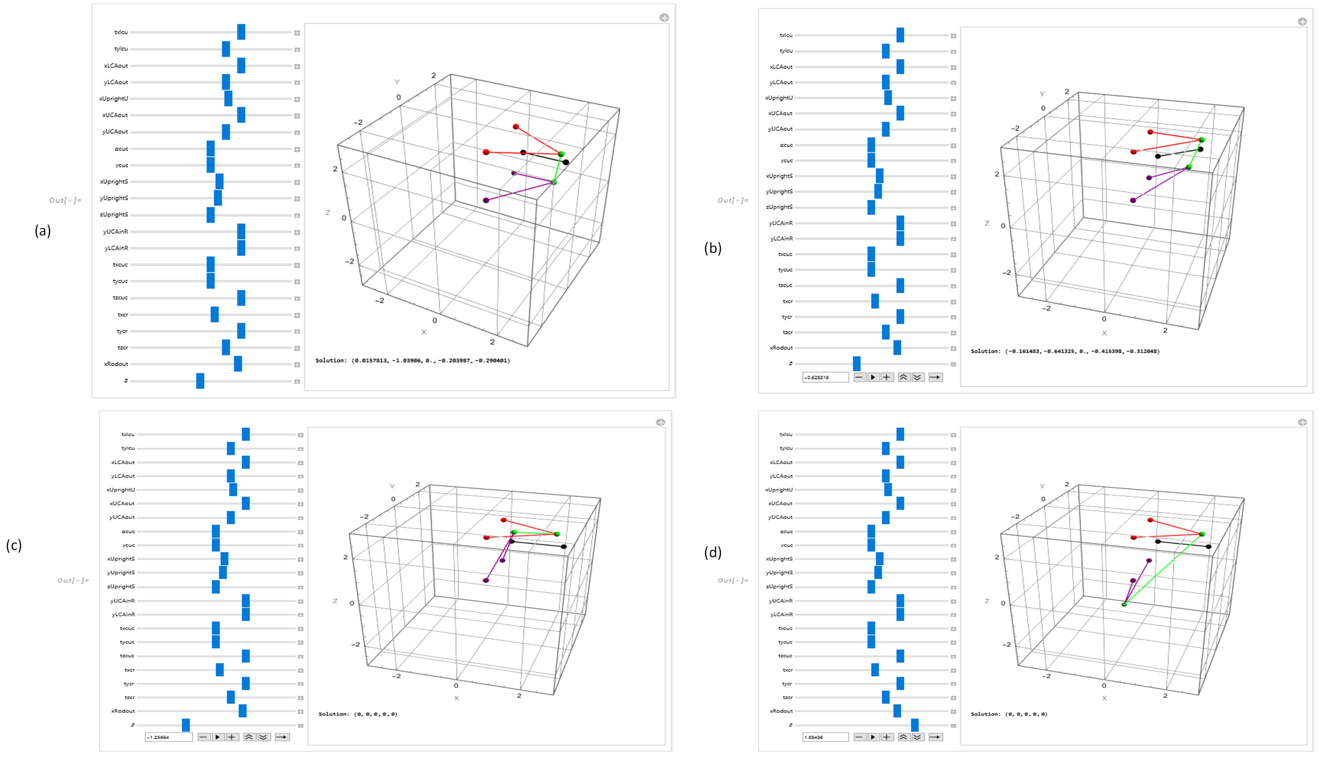
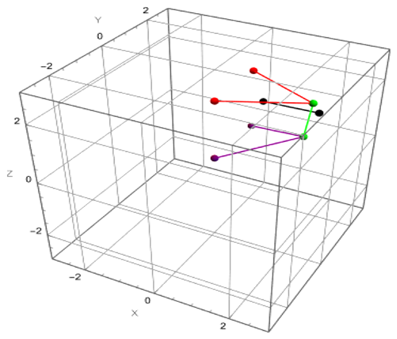
In color coding, red indicates the upper control arm, purple represents the lower control arm, green is used for the vertical upright connection, and black corresponds to the rod (such as a steering link or pushrod). The elements with a line[…] denotes mechanical links between components, while sphere[…, 0.1] is used to visualize joints or mounting points in the 3D suspension model.
The visualization function gives a general spatial view of the whole suspension assembly. It provides a clear view of how control arms, the upright, and linkages interact in three-dimensional space by color coding the major components and highlighting their joint locations. This visual tool not only aids in verifying model correctness but also supports further enhancements such as dynamic simulation, design optimization, and educational demonstrations. Furthermore, the flexible rendering pipeline allows for real-time updates to suspension geometry and articulation, which allowing the continuous integration of engineering feedback into the design process.

6. Dynamic Kinematic Solver

The section demonstrates how to model the physical behavior of a double wishbone suspension system under different geometric and alignment conditions by using the manipulate and NSolve constructs in the Wolfram language to create a dynamic solver. The tool enables users to modify chassis and component parameters in real time while solving the system of nonlinear equations that maintain mechanical linkage constraints. The visualization automatically updates to show each valid configuration so users can interactively examine different suspension designs and behaviors. To provide a concrete numerical basis for these simulations, a representative set of baseline parameters for the DWS system is defined in Table 2. These values establish a valid, initial geometric configuration that serves as a starting point for parametric exploration.
Figure 3 shows the results of a dynamic kinematic simulation for the double wishbone suspension model using a constraint-based solver. The system checks whether the upright, control arms, and rod links can meet spatial and mechanical constraints based on user-defined parameters. In successful cases (a and b), the solver produces consistent joint positions that result in a plausible suspension layout, as visually validated by the continuous and symmetric linkage geometry. In cases (c and d), the system is over- or under-constrained, and the solver fails to converge to a valid solution, which resulting in disconnected or distorted linkage representations. This shows the importance of constraint resolution in ensuring physical plausibility within dynamic simulations.
Module [ { solution , β cuc , α lcu , β lcu , γ lcu , β cr , γ cr , } , equations U = Thread pUprightU global [ ] = pUCAout global [ ] ; equations S = Thread pUprightS global [ ] = pRodout global [ ] ; deqs = ReplaceAll Join equations U , equations S , { } ; cons = { 0.5 β cuc 1.0 , π 2 α lcu π 2 , π β lcu 0 , 1.0 γ lcu 1.0 , π β cr π , 1.0 γ cr 1.0 } solution = NSolve Join [ deqs , cons ] , { } ; If solution , { } = solution [ [ 1 ] ] , { } = { 0 , 0 , 0 , 0 , 0 , 0 } ; drawSuspension [ updated parameters ] ]
The local scope defines a solution computation and storage area for NSolve together with the unknown joint angles β cuc (upper control arm orientation) and α lcu , β lcu , γ lcu (upright orientation through the lower control arm) and β cr , γ cr (tie rod orientation). The equations define kinematic constraints which show the positions that must match in 3D space for parts to be physically connected. The equationsU expression verifies that the upper point of the upright corresponds to the UCA outboard joint and the equationsS expression verifies that the upright side matches the tie rod outboard joint. The system becomes solvable through symbolic parameter replacement of manipulated counterparts which leads to a nonlinear system. The system requires domain constraints to prevent unrealistic movements of the upright and tie rod from occurring. The numerical solution of the system yields joint angle values that fulfill every constraint. A valid solution discovered during the process updates the visualization by showing the suspension system with new geometric and angular information to provide immediate feedback for parameter adjustments. The system defaults to a neutral configuration with zero angles when no solution is found to prevent visual display issues. The module includes sliders at its bottom for controlling mount point locations (like xLCAout, txcr, xRodout) as well as initial chassis/UCA orientation ( α , γ ) and suspension deflection angle ( β ). Users can modify design parameters through sliders to test arm length variations and mounting offset changes while examining how geometry influences suspension performance and feasibility in bump and compression simulations.

6.1. Performance and Computational Cost

The computational performance of this interactive framework, particularly the trade-off between real-time responsiveness and model complexity is important. The rendering of the suspension geometry via Graphics3D is computationally inexpensive and essentially instantaneous for a single, solved configuration. However, the real-time feel of the manipulate interface is directly dependent on the time required for NSolve to find a valid solution for each discrete step of a slider.
For most parameter adjustments within a well-constrained design space, the solver converges in a fraction of a second, providing a smooth, interactive experience. In contrast, when exploring parameter spaces that lead to complex or near-singular geometric configurations, NSolve may require more computational time to converge. This can result in a noticeable lag between a parameter adjustment and the visual update. Therefore, while the framework is a powerful tool for rapid design exploration, users should be aware that its real-time responsiveness is ultimately governed by the computational cost of solving the underlying nonlinear kinematic constraints at each step.

6.2. Analysis of Computational Complexity

The computational cost of the dynamic kinematic solver is primarily determined by the complexity of solving the system of nonlinear algebraic equations within the NSolve function. Performance does not scale linearly and is sensitive to several factors:
  • Problem Complexity and Size: The dominant factor is the size of the equation system, which is a function of the number of independent loops and constrained degrees of freedom in the mechanism. As more components or constraints are added (e.g., modeling both sides of the vehicle or adding complex anti-roll bar linkages), the number of simultaneous equations and variables grows, which can lead to a non-polynomial increase in the time required to find a solution.
  • Constraint Nonlinearity: The constraint equations are highly nonlinear, involving trigonometric functions (from the rotation matrices) and polynomial terms. The complexity of these equations directly impacts the difficulty of finding the roots of the system, which is the core task of the numerical solver.
  • Parameter Dimensionality: While the dimensionality of the user-controlled parameters (the sliders in Manipulate) does not increase the complexity of a single solution, it expands the solution space that can be explored. As noted previously, navigating to regions of this space corresponding to singular or near-singular configurations can significantly increase the time to convergence for the solver.
For the specific DWS model presented, the system size is small and well defined, allowing for near-real-time performance. However, scaling this approach to a full-vehicle model would require careful management of the model’s complexity to maintain interactive responsiveness.

6.3. Interactive Sensitivity Analysis

Although a formal quantitative sensitivity analysis, which would involve calculating the partial derivatives of output variables with respect to each input parameter, is outside the scope of this paper, the proposed framework facilitates a powerful form of qualitative, interactive sensitivity analysis.
The manipulate interface allows engineers to intuitively probe the system’s sensitivity. By making a small adjustment to a single input parameter via its slider (e.g., slightly changing a chassis mounting point), the user can instantly observe the magnitude of the resulting change in the suspension’s geometry, such as the wheel’s camber or toe angle. If a small parameter tweak causes a large, visible change in the output, the system is highly sensitive to that parameter in the current configuration. Conversely, if a large change results in minimal deviation, the system is robust to that input.
This immediate visual feedback provides an intuitive, real-time understanding of design sensitivities that is often more accessible during early-stage design than interpreting large tables of numerical sensitivity indices. It allows designers to quickly identify the most critical geometric parameters that govern suspension performance, enabling them to focus their optimization efforts more effectively.
The interactive simulation module converts the suspension model into an effective design and analysis instrument. The system enables users to see valid suspension configurations through numerical solutions in real time and 3D rendering of symbolic kinematic models. The system proves essential for design engineers who need to evaluate geometry changes, analyze motion constraints, and detect mechanical infeasibility during the early design stages. The module enables real-time exploration of geometry-to-behavior relationships, which makes it essential for the broader modeling framework and a fundamental component for suspension system optimization.

7. Conclusions

This paper presented a novel symbolically driven framework for 3D geometric modeling, constraint-based solving, and real-time visualization of a double wishbone suspension system framework through symbolic methods. The framework is making a significant contribution by using homogeneous transformations together with Euler-based rotation matrices and symbolic point definitions to construct suspension assemblies precisely and modularly within three-dimensional space. The framework, which combines symbolic kinematic representation with numerical constraint solving and dynamic rendering, establishes a major shift from conventional rigid-body modeling practices because they either fail to provide analytical clarity or real-time interactivity. The framework automatically determines internal degrees of freedom through user-defined geometry by applying nonlinear vector constraints to resolve upright and rod orientations. The system enables real-time visual validation of design choices while maintaining physical feasibility. The model becomes highly accessible through its integration with an interactive manipulation interface, which provides immediate feedback during parameter adjustments and enables engineers and students to explore suspension behavior through intuitive hands-on interaction.
Multiple use cases demonstrated how the framework successfully handled complex suspension configurations while showing their design under different conditions. The system demonstrated both geometric continuity and realistic articulated motion while delivering important insights about design variable impacts on camber and toe kinematic outcomes. The proposed system provides a solid foundation for future research and development. The immediate next steps will focus on rigorous validation to substantiate the framework’s practical applicability and accuracy. First, we will perform a comprehensive computational benchmark of the kinematic model. This will involve comparing key performance outputs, such as camber and toe curves, against results from industry-standard MBD software like Adams to quantitatively validate our geometric and constraint-based solver. This dynamic model can also be validated through direct comparison with experimental data obtained from a physical suspension test instrument or vehicle. Furthermore, the parametric nature of the framework makes it an ideal platform for integrating automated design optimization routines, using genetic algorithms or gradient-based methods to search the design space for geometries that optimize specific performance targets. These steps will transition the framework from a powerful kinematic analysis tool to a fully validated and predictive engineering design suite.

Author Contributions

Conceptualization, M.W.A. and S.L.; methodology, M.W.A. and S.L.; validation, M.W.A. and S.L.; formal analysis, M.W.A. and S.L.; writing—original draft preparation, M.W.A.; writing—review and editing, S.L. and D.Q.L.; supervision, S.L. and D.Q.L. All authors have read and agreed to the published version of the manuscript.

Funding

Authors disclose support for the research of this work from Ferrari and the European Union under the PNRR (National Recovery and Resilience Plan) under Grant No. 2933.

Institutional Review Board Statement

Not applicable.

Informed Consent Statement

Not applicable.

Data Availability Statement

The original contributions presented in this study are included in the article. Further inquiries can be directed to the corresponding authors.

Acknowledgments

We would like to express our sincere gratitude to the Ferrari Technical Team. T. Davide, F. Alessandro, and F. Rocco for their invaluable support to this research. Their expertise and assistance have been instrumental in completing this work.

Conflicts of Interest

The authors declare no conflicts of interest.

Abbreviations

The following abbreviations are used in this manuscript:
SymbolDescriptionType/Unit
α cuc Rotation angle (pitch) of upper control arm (UCA) in chassis frameAngle (radians)
β cuc Rotation angle (yaw) of UCA in chassis frame, solved dynamicallyAngle (radians)
γ cuc Rotation angle (roll) of UCA in chassis frameAngle (radians)
α lcu Rotation angle (pitch) of Upright in LCA frame, solved dynamicallyAngle (radians)
β lcu Rotation angle (yaw) of Upright in LCA frame, solved dynamicallyAngle (radians)
γ lcu Rotation angle (roll) of Upright in LCA frame, solved dynamicallyAngle (radians)
β Cr Yaw angle of tie rod (rod) in chassis frame, solved dynamicallyAngle (radians)
γ Cr Roll angle of tie rod (rod) in chassis frame, solved dynamicallyAngle (radians)
β Suspension bump angle/deflection used to drive motion
(applies to LCA)Angle (radians)
x UCAout X-coordinate of the UCA outboard connection in its local frameDistance (units)
y UCAout Y-coordinate of the UCA outboard connection in its local frameDistance (units)
x LCAout X-coordinate of the LCA outboard connection in its local frameDistance (units)
y LCAout Y-coordinate of the LCA outboard connection in its local frameDistance (units)
x UprightU X-offset of upright’s upper ball joint in upright local frameDistance (units)
x UprightS X-offset of upright’s side connection (tie rod or damper)Distance (units)
y UprightS Y-offset of upright’s side connection (tie rod or damper)Distance (units)
z UprightS Z-offset of upright’s side connection (if used in 3D placement)Distance (units)
y UCAinR Y-offset of UCA inboard mount (rail variant)Distance (units)
y LCAinR Y-offset of LCA inboard mount (rail variant)Distance (units)
t x cuc X-translation of UCA frame relative to chassisDistance (units)
t y cuc Y-translation of UCA frame relative to chassisDistance (units)
t z cuc Z-translation of UCA frame relative to chassisDistance (units)
t x lcu X-translation of LCA-to-upright joint in chassis (manipulated input)Distance (units)
t y lcu Y-translation of LCA-to-upright joint in chassisDistance (units)
t x cr X-offset of rod mount point in chassisDistance (units)
t y cr Y-offset of rod mount point in chassisDistance (units)
t z cr Z-offset of rod mount point in chassisDistance (units)
x Rodout X-length of rod (from inboard to outboard tip)Distance (units)
pUCAinF[…]Inboard frame-side point of upper control arm (global)3D Position
pUCAout[…]Outboard point of UCA, connects to upright3D Position
pLCAinF[…]Inboard chassis-side point of lower control arm (global)3D Position
pLCAout[…]Outboard point of LCA, connects to upright3D Position
pUprightU[…]Upper upright point where UCA connects3D Position
pUprightS[…]                                Side upright point (tie rod or damper connection)3D Position
pRodinglobal[…]Inboard (chassis-mounted) end of rod3D Position
pRodoutglobal[…]Outboard (upright-connected) end of rod3D Position
drawSuspension[…]Visualization function to render the entire suspension
system using all calculated pointsGraphics3D
solutionOutput of NSolve used to extract valid joint anglesList
equationsU, equationsSConstraint equations that ensure connected
parts meet at a common pointEquation Set
deqsMerged constraint equations from both UCA and tie rod systems       Equation Set
consConstraints on angle ranges for physically plausible behaviorInequality Set
NSolve[…]Numerical solver used to solve nonlinear constraint systemSolver Output

References

  1. Dubey, A.D.; Verma, S.; Kumar, P. Analysis of Double Wishbone Suspension System Using MechAnalyzer. In Advances in Mechanical and Energy Technology; Yadav, S., Jain, P.K., Kankar, P.K., Shrivastava, Y., Eds.; Springer: Singapore, 2022; pp. 245–255. [Google Scholar] [CrossRef]
  2. Park, H.; Langari, R.; Yi, H. Design and testing of double-wishbone suspension for enhanced outdoor maneuver stability of a six-wheeled mobile robot. Mechatronics 2024, 103, 103237. [Google Scholar] [CrossRef]
  3. Taneva, S.; Ambarev, K.; Penchev, S. Strength and Frequency Analysis of the Lower Arm of a Double Wishbone Suspension of a Passenger Car. ETR 2024, 1, 352–357. [Google Scholar] [CrossRef]
  4. Sharma, R. Design and Optimisation of Double Wishbone Suspension for High Performance Vehicles. Int. J. Veh. Syst. Model. Test. 2023, 17, 185–195. [Google Scholar] [CrossRef] [PubMed]
  5. Niu, Z.; Jin, S.; Wang, R.; Zhang, Y. Geometry Optimization of a Planar Double Wishbone Suspension Based on Whole-Range Nonlinear Dynamic Model. Proc. Inst. Mech. Eng. Part D J. Automob. Eng. 2022, 236, 3–14. [Google Scholar] [CrossRef]
  6. Avi, A.G.; Carboni, A.P.; Stella Costa, P.H. Multi-Objective Optimization of the Kinematic Behaviour in Double Wishbone Suspension Systems Using Genetic Algorithm; SAE Technical Paper 2020-36-0154; SAE: Warrendale, PA, USA, 2021. [Google Scholar] [CrossRef]
  7. Shao, Y.; Li, G.; Wang, J. Optimization Design of Double Wishbone Front Suspension Based on Dynamic Simulation. Appl. Sci. 2023, 14, 1812. [Google Scholar] [CrossRef]
  8. Arshad, M.W.; Lodi, S.; Liu, D.Q. Multi-Objective Optimization of Independent Automotive Suspension by AI and Quantum Approaches: A Systematic Review. Machines 2025, 13, 204. [Google Scholar] [CrossRef]
  9. Arshad, M.W.; Lodi, S. Quantum computing in the automotive industry: Survey, challenges, and perspectives. J. Supercomput. 2025, 81, 1093. [Google Scholar] [CrossRef]
  10. Upadhyay, P.; Deep, M.; Dwivedi, A.; Agarwal, A.; Bansal, P.; Sharma, P. Design and analysis of double wishbone suspension system. IOP Conf. Ser. Mater. Sci. Eng. 2020, 748, 012020. [Google Scholar] [CrossRef]
  11. Golightly, D.; Pierce, K.; Palacin, R.; Gamble, C. A feasibility assessment of multi-modelling approaches for rail decarbonisation systems simulation. Proc. Inst. Mech. Eng. Part F J. Rail Rapid Transit. 2021, 236, 115–126. [Google Scholar] [CrossRef]
  12. Simpack Multibody Simulation Software. (n.d.). SIMULIA. Available online: https://www.3ds.com/products/simulia/simpack (accessed on 1 March 2025).
  13. Wang, J.; Zhao, Y. A repelling-screw-based approach for the construction of Jacobian matrices in parallel manipulators. Mech. Mach. Theory 2022, 170, 104726. [Google Scholar] [CrossRef]
  14. Guo, M.; De Persis, C.; Tesi, P. Data-Driven Stabilization of Nonlinear Systems via Taylor’s Expansion. In Lecture Notes in Control and Information Science; Postoyan, R., Frasca, P., Panteley, E., Zaccarian, L., Eds.; Springer: Cham, Switzerland, 2024; pp. 299–315. [Google Scholar] [CrossRef]
  15. Ashtekar, V.; Bandyopadhyay, S. Forward Dynamics of the Double-Wishbone Suspension Mechanism Using the Embedded Lagrangian Formulation. In Mechanism and Machine Science; Sen, D., Mohan, S., Ananthasuresh, G.K., Eds.; Springer: Singapore, 2021; pp. 843–859. [Google Scholar] [CrossRef]
  16. Zhang, B.; Li, Z. Mathematical modeling and nonlinear analysis of stiffness of double wishbone independent suspension. J. Mech. Sci. Technol. 2021, 35, 5671–5680. [Google Scholar] [CrossRef]
  17. Adams: The Multibody Dynamics Simulation Solution. (n.d.). Enteknograte. Available online: https://enteknograte.com/adams-multibody-dynamics-simulation-solution/ (accessed on 1 February 2025).
  18. Wolfram Research. (n.d.). Symbolic and Numeric Computation. Wolfram U. Available online: https://www.wolfram.com/wolfram-u/courses/mathematics/symbolic-numeric-computation-math915/ (accessed on 18 February 2025).
  19. Wolfram Research. (n.d.). Advanced Manipulate Functionality. Wolfram Language Documentation. Available online: https://reference.wolfram.com/language/tutorial/AdvancedManipulateFunctionality.html (accessed on 18 February 2025).
  20. Larcher, M.; Stocco, D.; Tomasi, M.; Biral, F. A Symbolic-Numerical Approach to Suspension Kinematics and Compliance Analysis. In Proceedings of the ASME 2024 International Mechanical Engineering Congress and Exposition. Volume 5: Dynamics, Vibration, and Control, Portland, OR, USA, 17–21 November 2024; p. V005T07A049. [Google Scholar] [CrossRef]
  21. Uchida, T.; McPhee, J. Driving Simulator with Double-Wishbone Suspension Using Efficient Block-Triangularized Kinematic Equations. Multibody Syst. Dyn. 2012, 28, 331–347. [Google Scholar] [CrossRef]
  22. Chun, H.-H.; Tak, T.-O. Sensitivity Analysis Using a Symbolic Computation Technique and Optimal Design of Suspension Hard Points. J. Korean Soc. Precis. Eng. 1999, 16, 26–36. [Google Scholar]
  23. Makita, M. An Application of Suspension Kinematics fMontreal, Quebec H3G 1M8, Canadaor Intermediate Level Vehicle Handling Simulation. JSAE Rev. 1999, 20, 471–477. [Google Scholar] [CrossRef]
  24. Balike, K.P. Kineto-Dynamic Analyses of Vehicle Suspension for Optimal Synthesis. Ph.D. Thesis, Concordia University, Montreal, QC, Canada, 2010. [Google Scholar]
Figure 2. The schematic diagram illustrates the positional connections between the upper and lower control arms (UCA and LCA), upright, rod linkage, and steering input components. The model includes annotated local coordinate axes together with reference points that label each element (such as pUCAout, pUprightS, and pRodout). The parameter names xUCAout, yLCAinR, and xUprightS represent adjustable geometric values in their respective frames. The diagram shows the component frames (UCA frame, LCA frame, upright frame) and their transformations and connections through joint locations and linkage endpoints relative to the global reference frame.
Technologies 13 00332 g002
Figure 3. The kinematic solver successfully identifies valid solutions for all geometric constraints in panels (a,b), which produce physically correct component linkage visualizations. The constraint-solving system fails to find valid solutions in panels (c,d) because the input parameters lead to visibly incorrect linkage alignment and disconnected joints. In the visualizations, the red and purple lines represent the upper and lower control arms, respectively. The green line represents the upright (knuckle), and the black line represents the tie rod.
Technologies 13 00332 g003
Figure 4. Three-dimensional geometric visualization of a valid double wishbone suspension configuration. The rendered suspension system shows proper alignment and articulation of the upper and lower control arms (red and purple), the upright (green), and associated links such as tie rods (black). All components are connected and meet geometric and kinematic constraints, which shows a physically consistent assembly under the given parameter set.
Technologies 13 00332 g004
Table 2. Baseline geometric parameters from the manipulate function. Each parameter has an input range of either [ 5 , 5 ] or [ π , π ] , with the initial/default value listed.
ParameterBaseline ValueRange
txlcu 2.0 [ 5 , 5 ]
tylcu 1.0 [ 5 , 5 ]
xLCAout 2.0 [ 5 , 5 ]
yLCAout 1.0 [ 5 , 5 ]
xUprightU 1.2 [ 5 , 5 ]
xUCAout 2.0 [ 5 , 5 ]
yUCAout 1.0 [ 5 , 5 ]
α cuc 0.0 [ π , π ]
γ cuc 0.0 [ π , π ]
xUprightS 0.6 [ 5 , 5 ]
yUprightS 0.5 [ 5 , 5 ]
zUprightS 0.0 [ 5 , 5 ]
yUCAinR 2.0 [ 5 , 5 ]
yLCAinR 2.0 [ 5 , 5 ]
txcuc 0.0 [ 5 , 5 ]
tycuc 0.0 [ 5 , 5 ]
tzcuc 2.0 [ 5 , 5 ]
txcr 0.3 [ 5 , 5 ]
tycr 2.0 [ 5 , 5 ]
tzcr 1.0 [ 5 , 5 ]
xRodout 1.8 [ 5 , 5 ]
β −0.4 [ π , π ]
Disclaimer/Publisher’s Note: The statements, opinions and data contained in all publications are solely those of the individual author(s) and contributor(s) and not of MDPI and/or the editor(s). MDPI and/or the editor(s) disclaim responsibility for any injury to people or property resulting from any ideas, methods, instructions or products referred to in the content.

