Abstract
This paper presents a novel cochlear implant (CI) sound coding strategy called Spectral Feature Extraction (SFE). The SFE is a novel Fast Fourier Transform (FFT)-based Continuous Interleaved Sampling (CIS) strategy that provides less-smeared spectral cues to CI patients compared to Crystalis, a predecessor strategy used in Oticon Medical devices. The study also explores how the SFE can be enhanced into a Temporal Fine Structure (TFS)-based strategy named Spectral Event Extraction (SEE), combining spectral sharpness with temporal cues. Background/Objectives: Many CI recipients understand speech in quiet settings but struggle with music and complex environments, increasing cognitive effort. De-smearing the power spectrum and extracting spectral peak features can reduce this load. The SFE targets feature extraction from spectral peaks, while the SEE enhances TFS-based coding by tracking these features across frames. Methods: The SFE strategy extracts spectral peaks and models them with synthetic pure tone spectra characterized by instantaneous frequency, phase, energy, and peak resemblance. This deblurs input peaks by estimating their center frequency. In SEE, synthetic peaks are tracked across frames to yield reliable temporal cues (e.g., zero-crossings) aligned with stimulation pulses. Strategy characteristics are analyzed using electrodograms. Results: A flexible Frequency Allocation Map (FAM) can be applied to both SFE and SEE strategies without being limited by FFT bandwidth constraints. Electrodograms of Crystalis and SFE strategies showed that SFE reduces spectral blurring and provides detailed temporal information of harmonics in speech and music. Conclusions: SFE and SEE are expected to enhance speech understanding, lower listening effort, and improve temporal feature coding. These strategies could benefit CI users, especially in challenging acoustic environments.
1. Introduction
The groundbreaking Continuous Interleaved Sampling (CIS) strategy reported in [1,2] allowed significant improvements in speech understanding for cochlear implant (CI) users. CI technology has gradually matured into a device capable of providing around 80% of sentence recognition for users in quiet environments [3].
However, the performance of cochlear implants varies significantly across individuals and tends to deteriorate in complex listening environments, such as those with background noise [4,5]. Additionally, music appreciation remains generally poor [6]. These limitations can be partially attributed to the coding strategies implemented in CI devices. Among various constraints, the mismatch between anatomical (tonotopic) and clinical (i.e., related to CI) frequency allocation maps (FAMs), along with spectral blurring, are two important factors that require improvements in electrical stimulation within CIS-based coding strategies.
In current CI technologies based on fast Fourier transform (FFT) for signal analysis, a key limitation is that electrode bandwidths must align with FFT bin sizes, with the minimum possible bandwidth being equal to a single bin. This constraint, combined with the limited angle of electrode insertion into the cochlea, aggravates the misalignment between natural tonotopic and clinical frequency maps [7].
It has been demonstrated that reducing frequency mismatch leads to better pitch perception and improved lateralization [8,9]. Providing a more flexible FAM can help mitigate this mismatch by appropriately adjusting the assigned bandwidth for each electrode.
FAM plays an important role in improving vowel recognition, pitch perception, and melody recognition [10]. Researchers have examined different filter spacings to enhance speech and music perception. Some have explored the effects of increasing the number of channels at lower frequencies (note that this approach is not applicable to coding strategies with a minimum FAM value equal to the bandwidth of a single FFT bin). For instance, Geurts and Wouters (2004) [11] proposed a novel filterbank that allocated more filters to the low frequencies, aiming to improve place coding of harmonics and thus enhance pitch perception. Their study revealed lower detection thresholds for F0 in synthetic vowel stimuli compared to a conventional log-spaced filterbank. Other studies have suggested that assigning more electrodes to frequencies within the range of the first two vowel formants (i.e., F1 and F2) may improve speech perception [12,13]. Tabibi et al. [14] proposed the use of a physiologically based Gammatone filterbank with higher resolution in lower-frequency channels, demonstrating improvements in melody contour identification tasks for CI recipients. Finally, filterbanks spaced according to a musical scale (e.g., semitone spacing) have been shown to enhance place coding of individual harmonics, thereby improving melody recognition and melody quality [15,16]. All these studies highlight the importance of flexibility in defining FAM within CI coding strategies.
Spectral blurring, caused by poor extraction of frequency information, can reduce the effectiveness of CI coding strategies [17]. Efforts to mitigate spectral blurring through current steering [18,19] have demonstrated measurable improvements for most CI recipients. The spectrum of the acoustic input signal exhibits varying levels of sharpness, depending on the nature of the signal (e.g., some signals behave almost sinusoidally, while others have broader spectral profiles). By extracting spectral features, one can calculate this “sharpness” and provide the appropriate inner-ear current spread required by the specific signal. The objective should be to closely approximate natural hearing, as suggested by Nogueira et al. [20].
This article introduces a coding strategy methodology named Spectral Feature Extraction (SFE) that integrates effectively with FFT-based CIS strategies and enhances them by addressing the aforementioned limiting factors. SFE is developed based on the hypothesis that a sharper spectral representation might help some CI users focus more effectively on salient spectral features of the input signal. The primary advantages of the SFE sound coding methodology include the following:
- A flexible frequency allocation that allows advanced FAM fitting methods to adopt anatomically inspired approaches to optimize hearing performance. Furthermore, as technology evolves, this feature can meet the needs of electrode arrays with higher numbers of contacts, requiring precise and narrow low-frequency bandwidths.
- A more precise extraction of spectral features for electrical stimulation, minimizing the spectral blurring effect, ensuring that signals with narrow-band harmonics stimulate only the relevant electrode as defined in the clinical FAM.
- A method to measure the similarity between the frequency content of the analyzed signal and that of a sinusoid signal at a given frequency, using a metric of spectral sharpness, enabling the encoding of spectral features more efficiently.
In this article, we also demonstrate how the SFE coding strategy can be refined into a Temporal Fine Structure (TFS)-based strategy called Spectral Event Extraction (SEE). Providing low-frequency TFS information is challenging in CIS coding strategies with wide FFT bins. The SFE’s capability to process sub-band FFT bins and deliver more accurate frequency estimations, positions it as an effective framework for encoding the TFS of input signals with multiple narrowband components. Furthermore, advancements like distributed all-polar (DAP) stimulations [21] and electrode arrays placed near the modiolus [22], which may allow for more focused stimulations, underscore the importance of adopting TFS-based strategies. According to Moore et al., delivering temporal cues to the ear represents an improved approach to sound coding in cochlear implants (CI) [23]. Over the last decade, efforts have been made to offer TFS to CI recipients [24,25,26]. Some clinical studies have shown that the success of TFS-based strategies varies significantly among individuals and is not necessarily superior to envelope-based strategies [27,28]. However, other studies indicate a preference for TFS-based coding for vowel monosyllables, speech, and music [29,30].
The SEE strategy proposed in this article combines the high spectral resolution of the SFE with TFS encoding of the input signals. Unlike other TFS-based strategies that rely on direct temporal analysis of the input signal, SEE employs an FFT-based methodology. This approach introduces a spectral feature tracking mechanism to ensure consistent zero-crossing events across successive windowed frames.
This manuscript encompasses (i) a detailed description of the SFE coding strategy; (ii) an explanation of the SEE coding strategy; and (iii) analyses of the output electrodograms generated by applying SFE and SEE over pre-recorded wave files (referred to as “numerical simulations” in this study). It is noteworthy that the SFE strategy has been employed in an acute-testing clinical investigation conducted by Zhang et al. [31], where it was compared to the Crystalis strategy. While Zhang et al. [31] primarily focused on experimental evaluation and provided only a high-level overview of the SFE strategy, the present manuscript aims to offer a more comprehensive and detailed description of SFE, as well as to introduce a method for extending it to support a TFS-based approach (i.e., SEE).
2. Materials and Methods
In this section, we detail the technical aspects of our proposed Spectral Feature Extraction (SFE) coding strategy, and the methodologies (both numerical simulation and clinical) used to analyze its behavior. The SFE shares some processing blocks with the Crystalis strategy, a commercial sound coding strategy used in Oticon Medical CI devices [32,33]. Unlike Crystalis, which imposes constraints on FAM settings, the SFE offers complete flexibility in the FAM, ensuring that bandwidths are not limited to multiples of FFT bins. Additionally, it significantly reduces spectral blurring.
Another topic covered in this section is Spectral Event Extraction (SEE), a TFS-equipped variant of the SFE strategy. In SEE, the concept of spectral features is replaced by spectral events that incorporate the aspect of timing.
2.1. Spectral Feature Extraction (SFE) Strategy
Figure 1 illustrates the main processing blocks of the SFE strategy, from receiving audio stimuli to generating stimulation pulses. The SFE and Crystalis strategies primarily differ in the analysis and regrouping of the spectral contents of the input signal. In SFE, frequency analysis is performed in the Synthetic Feature eXtraction (SFX) block, and regrouping is handled by the Feature to Channel (F2C) assignment block. The remaining processing blocks, such as pre-processing, N-of-M channel selection, XDP compression, and CIS pulse frame generation, are similar between the two strategies. These blocks are explained in the Appendix A.
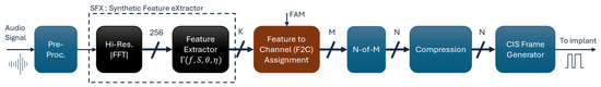
Figure 1.
Signal processing blocks in the SFE coding strategy. The blocks are color-coded to indicate their relationship to the Crystalis simulation chain: blue for unchanged blocks, brown for modified blocks, and black for newly introduced blocks.
2.1.1. Synthetic Feature eXtraction (SFX) Block
The SFX block is the frequency analyzer in the SFE strategy. It is designed based on the following guidelines: (1) reducing frequency smearing and improving the resolution of estimated frequency terms; (2) extracting important spectral features rather than the most energetic terms; (3) supporting FAM with FFT sub-band bin size.
In the SFX block, the input signal (sampling frequency fs = 16 kHz) is firstly windowed using a Kaiser window (16 msec, 256 samples, β = 6.9) and then important spectral features (FFT-based) of the windowed signal are extracted. The β parameter in the Kaiser window allows bandwidth adjustment independently of window length. Setting β = 6.9 yields a bandwidth similar to a 256-sample Hanning window. The philosophy behind SFX is that the ‘Features’ of spectral ‘Peaks’ convey the most important information of the acoustic signal. Spectral peaks correspond to the dominant frequency components of a signal. These peaks often represent the most perceptually and functionally significant features—such as formant frequencies in speech, which are crucial for vowel identification, and harmonic structures in music, which are closely tied to pitch perception.
For each spectral peak there is a feature vector represented by energy , phase , frequency , and confidence parameters (i.e., ). The first three parameters in each feature vector aim to represent the corresponding FFT peak by a ‘Synthetic’ spectral peak of the windowed (i.e., Kaiser) sinusoidal signal.
The confidence parameter indicates how similar the synthesized peak is to the FFT of a sinusoid at that frequency multiplied by the Kaiser window. Periodicity and stochasticity are two factors that affect the confidence level, increasing or decreasing it, respectively. If the acoustic signal is a pure tone, both the original and synthetic spectral peaks resemble a smeared peak (i.e., the spectrum of the window used in the FFT) centered at the frequency of the sinusoidal signal, therefore . Stochasticity causes the original peak to deviate from the synthetic peak. When the peaks are not similar, there is less confidence in the estimated energy, phase, and frequency of the original peak.
The SFX incorporates three complementary methods to precisely obtain the spectral peaks: (i) using a longer FFT window, (ii) calculating a high-resolution FFT, and (iii) feature extraction using a de-smearing method.
- (A)
- Long-windowed high-Resolution FFT
The SFX uses a 16 msec normalized Kaiser window (N = 256), which is twice the length of the Hanning window in Crystalis (N = 128). This increases the frequency resolution of the spectral peaks by a factor of two. Further increasing the window length to N > 256 may degrade the temporal resolution for high-frequency terms. The SFX performs a 2N-point (i.e., 512-point) double-FFT on an N-point windowed signal, zero-padded by N samples. This method does not degrade the temporal resolution while generating interpolated FFT samples. Theoretically, this method is equivalent to multiplexing two N-point FFT spectra [34]: one calculated on the original signal and one calculated on a half-bin shifted signal in the frequency domain, as presented in Figure 2.
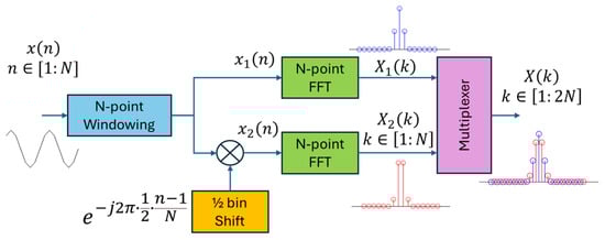
Figure 2.
Doubling the FFT resolution by multiplexing two N-point FFTs: one computed on the original signal (i.e., ), and the other on a half-bin shifted version of the signal (i.e., ). This process is equivalent to performing a 2N-point FFT on an N-point zero-padded, windowed signal (i.e., where is a zero vector of length N.
The peaks are identified using the high-resolution 2N-point spectrum. The SFX collects up to K peaks (default: K = 22) using local maximum samples (see Figure 3a). Notably, the selected peaks have equal or higher energy values than their adjacent samples. This distinguishes the SFX from Crystalis, where the most energetic spectral samples are selected without necessarily being local maxima.
- (B)
- Feature extraction by de-smearing
The SFX extracts a feature vector for each identified spectral peak through a refinement process that de-smears the peak—originally spread across multiple frequency domain samples—until it is represented as a Dirac impulse at the frequency . This is performed by analyzing the numerical values of ±2 FFT samples adjacent to each identified peak at index C (see Figure 3b). In this de-smearing process, it is assumed that a pure tone sinusoidal signal with frequency may have a value not necessarily located at the identified peak at index C. The values of the adjacent samples can then be analyzed to find the precise location of and its peak energy, assuming that the adjacent samples are sparse samples from the power spectrum of the window (i.e., Kaiser spectrum) around .
The refinement process has been shown for three examples in Figure 3b. Two extreme cases correspond to cases where and FFT peak coincide (top), and where is ½-bin deviated (bottom). The middle panel shows a case in between. The SFX estimates and the peak energy by measuring the symmetry of FFT samples around sample C (i.e., FFT peak) using absolute relative values of adjacent samples (i.e., ).
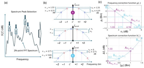
Figure 3.
Synthesis of high-resolution features. (a) K spectral peaks are selected from the double-FFT analysis. (b) De-smearing is performed using the main lobe characteristics of the Kaiser window spectrum and the difference values between four adjacent spectral samples in the double-FFT, denoted as . Point A (top) and Point B (bottom) correspond to two extreme conditions: one where the peak frequency aligns with an FFT sample (index C), and another where it lies between two adjacent samples. The plot in the middle represents an intermediate condition. The values in set vary depending on the relative position of the peak with respect to the double-FFT samples. (c) Mapping functions and to calculate the frequency and energy spectrum corrections that should be applied to FFT sample C to accurately represent the true peak frequency and energy. The mapping values for the indicated Point A (pink) and Point B (cyan) are shown over the functions for different values of indicated in (b).
Each is used to calculate an energy () and a frequency ( compensation that should be applied to the FFT peak to estimate the final energy and frequency of the synthetic peak.
Hz is the frequency resolution (i.e., frequency bin spacing) of the double-FFT, and is the compensation needed to place the passband lobe of the normalized Kaiser spectrum at 0 dB. This ensures that the spectral peak amplitude directly represents the sound level corresponding to that peak. The function maps each to a frequency compensation (Figure 3c). This function is obtained numerically by determining the frequency shift that must be applied to the Kaiser spectrum so that it exhibits an energy difference between two samples that are one bin apart (i.e., one bin in the double-FFT spectrum).
The marked points on correspond to Point A, which represents the case where the peaks overlap (i.e., ). In this case dB. These values map to bin, and thus bin upon Equation (1). As a result, in average the FFT-bin C should be shifted bin to map to . For marked points that correspond to ½-bin frequency deviation between the peaks, dB, bin, and thus bin. This means that the FFT-peak should shift bin to map to .
To correct the energy of the peak, the function (Figure 3c) maps the frequency shift measured by to the power adjustment needed to be added to FFT energy values . This function is the inverted shape of the Kaiser spectrum. Note that in Equation (2), only two FFT samples are used to correct the energy because the two central samples provide more robust estimate for the energy compensation than the other off-centers samples.
Concerning the phase of the synthetic peak (), it is obtained by a linear regression fit to the unwrapped phase values of samples adjacent to the double-FFT peak location. The phase at the estimated peak center frequency, , is then calculated on this fit, as illustrated in the example shown in Figure 4a. In our numerical simulations, we limited the interpolation to a one-bin-apart neighborhood (i.e., a total of three samples).
Finally, the confidence is calculated through morphology analysis of the double-FFT samples around the FFT bin at index C. If these samples resemble a Kaiser spectrum, it is likely that the identified peak corresponds to a narrow-band signal around . Mathematically, this confident value can be expressed using the following equation:
is the standard deviation of the vector, and = 0.5774 is a normalization factor, setting the range of between 0 and 1. The confidence value approaches 1 when all four elements of the vector yield similar estimates, indicating strong agreement. Conversely, decreases when there is significant disagreement among the estimates. The value of corresponds to the maximum possible standard deviation of the vector, which occurs when bin—a case that represents the lowest level of agreement among the estimates. Figure 4b,c illustrate how modifications to FFT samples near a spectral peak can affect the estimated and the confidence value .
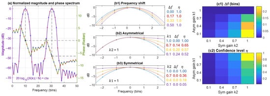
Figure 4.
(a) Normalized magnitude and phase spectrum of a signal containing two sinusoidal components with zero phase. 2N-point FFT samples are shown as blue and red dots. The peak frequency of the first component is located at an extremum FFT sample, while the second peak is located between two FFT samples. The phase is estimated using linear interpolation on the unwrapped phase values at the estimated . In this example, the interpolation yields 0 and . Phase wrapping maps these values to rad. (b,c) The effect of modifying the FFT spectrum around the peak on the estimated and confidence value . (b1) shifting the Kaiser spectrum consistently provides an error-free estimation of with a confidence value of . (b2) The spectrum (in log scale) is modified asymmetrically by multiplying one side with a gain factor . Decreasing the gain shifts the estimated frequency to the right side of the FFT peak, while decreases. (b3) Symmetric modification of the spectrum using a gain does not affect , but decreases as the spectrum flattens (i.e., transition from a peak to a flat spectrum, as in white noise). (c1,c2) Combined effects of asymmetric and symmetric gain modifications ( and ) on and , respectively.
2.1.2. Feature-to-Channel Assignment
The Feature-to-Channel (F2C) assignment block selects the most relevant feature for each channel from the K available features provided by the SFX block. It assigns at most one feature vector to each channel, with each channel representing an electrode on the CI array (e.g., M = 20). The assignment is performed using (i) the FAM of the electrodes that is not necessarily multiples of the FFT bins, and (ii) the frequency and energy parameters of the feature vectors. The phase and confidence parameters do not contribute to the F2C process; they are transferred along with other parameters in the feature vector to subsequent processing stages as accompanying parameters.
In the F2C block, the FAM is used to construct a frequency selector mask (FSM) for each channel (Figure 5). By default, FSMs resemble overlapped trapezoid functions with cross points determined by the FAM of the electrode array [19,35]. Features whose frequencies fall within a trapezoid mask compete for assignment to the corresponding channel. The feature providing the highest energy value after being scaled by the FSM function is selected. The F2C block assigns at most one winning feature vector to each channel. Features whose frequencies fall within the transition bands of FSMs are candidates for two adjacent channels.
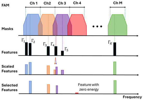
Figure 5.
Feature-to-Channel assignment process. The trapezoid FSM is formed from the FAM. Scaled features by FSM compete to be selected for each channel. In this example, and compete for channel 1. The scaled has a greater value so it is selected. competes with for channel 2 and with for channel 3. A zero-energy feature is assigned to a channel without any feature inside.
2.2. Spectral Event Extraction (SEE) Strategy
The Spectral Event Extraction (SEE) strategy is a modified version of the SFE strategy, extending features to events. Features in SFE lack temporal fine structure (TFS) information for stimulation, whereas in SEE, they include timestamped events that convey TFS information. The phase, frequency, and energy parameters in a feature vector do not specify explicitly when stimulation events should be generated so that they become synchronized with their corresponding synthetic tones. Consequently, the TFS information of the input signals is not preserved in the SFE strategy. The SEE addresses this issue by synchronizing stimulation events with synthetic signals at a given phase value (e.g., zero-crossing).
The SEE includes an event extractor block positioned between the SFX block and subsequent processing blocks (Figure 6). It receives K features from the SFX block and generates L ≤ K timestamp events , where is the onset time of the event. This time parameter is derived from the frequency and phase parameters (described in Section 2.2.1), while the other parameters retain the values provided by the feature vector. The events serve the same role as features for the subsequent processing blocks, which is why the F2C block is renamed to the Event-to-Channel (E2C) block. The SEE strategy uses an adapted (modified) N-of-M block. In the next sections, the event generator and the SEE-adapted N-of-M blocks are described.
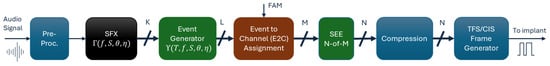
Figure 6.
Signal processing blocks in the SEE coding strategy. The blocks are color-coded to reflect their relationship to the Crystalis and/or SFE strategies: blue for unchanged blocks, brown and black for blocks that are modified and newly introduced, respectively, relative to Crystalis, and green for blocks specifically designed for SEE that are either new or differ from those in SFE.
2.2.1. Event Generator Block
The event generator block tracks features across frames to determine the timestamps of stimulating pulses. The timestamps correspond to moments when the phase of the synthetic tone crosses a predetermined level (e.g., zero crossing). The event generator links related features based on their frequency proximity. Without such links, zero-crossings calculated in each frame may result in inconsistent time events due to the nature of the FFT, which is performed over independently windowed segments of the signal.
The tracking mechanism is a precision-based approach used in the event generator, specifically within the SEE strategy. In the absence of tracking or under missed tracking conditions, SEE still generates pulses based on their estimated phase values, but without linking them to corresponding pulses from previous time frames. The SFE and SEE electrodograms are identical in terms of pulse amplitude and the envelope of the stimulating pulses. The main difference lies in the micro-structural timing precision of pulse delivery, which is unique to the SEE strategy. In contrast, SFE delivers pulses at fixed intervals.
Figure 7a illustrates the concept of feature tracking across four frames. Any two features in consecutive frames may be linked if the feature in frame n + 1 is in the frequency search region of the feature in frame n. Each feature in frame n + 1 can be assigned to only one feature in frame n. If multiple candidate features are available for linking, the one with the lowest frequency is selected. Figure 7b shows an example of linked features feat1 and feat2 represented by ( = 250 Hz, = 0 Radian) and ( = 280 Hz, = 3.27 Radian), respectively. The first zero-crossing occurs at t = 0. To find the next zero-crossing (at t = 3.8 msec), it must first be verified if the initial phase of feat2 (i.e., = 3.27) falls within the valid range of ending-phase of feat1. This range corresponds to the ending-phase of the lower and upper search frequencies for feature linkage. If the initial phase of feat2 is within this range, it is accepted; otherwise, it is adjusted to or depending on relative frequency values of feat2 and feat1.
Following the stabilization of phases by the tracking process, an event is created for any feature that produces a zero-crossing in the same frame. The event takes its accompanying parameters from the corresponding feature.
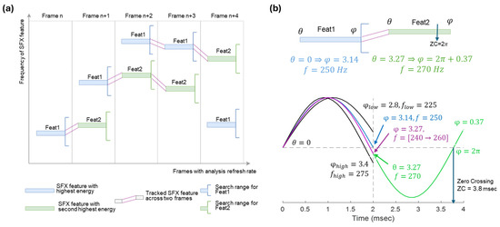
Figure 7.
Feature tracking. (a) Features are tracked based on their frequency vicinity in successive frames. (b) Event generation in two linked features feat1 and feat2. The ending-phase of feat1 (with = 250 Hz) is = 3.14 Rad, which is slightly lower than the initial phase of feat2 ( = 3.27). As is between 2.8 and 3.45 Rad (i.e., the minimum and maximum ending-phases), it is validated. In this toy example, this phase value corresponds to the ending-phase of a chirp linearly increasing from 240 Hz to 260 Hz in 2 msec during frame n. The validated = 3.27 and the frequency of feat2 (with = 270 Hz) determines a zero-crossing at = 3.8 − 2.0 = 1.8 msec with respect to frame n + 1.
2.2.2. N-of-M Block (Adapted to SEE)
In the SEE coding strategy, the event rate varies across channels. Low-frequency channels have fewer events than high-frequency channels. When there is no event for a low-frequency channel, a standard N-of-M may select a high-frequency, low-energy event because it always selects a fixed number of channels per frame. This random selection of low-energy, high-frequency channels can potentially result in noisy stimulation. To address this issue, a SEE-adapted N-of-M block reserves channels for a period of time after they are selected by the N-of-M in a previous frame. This reserved time can be set to one period of the event frequency (e.g., 4 ms for an event corresponding to f = 250 Hz) or to a fixed value for each channel. During the reserved time, the N-of-M counts the reserved channel as a selected channel (Figure 8).
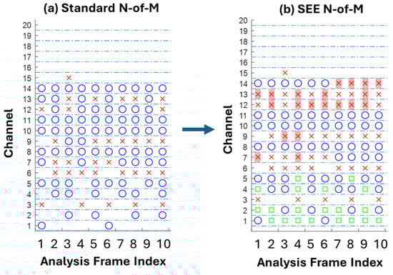
Figure 8.
Channels (ordinate) selected (blue), deactivated (red) and reserved (green) in standard N-of-M (a) and SEE-adapted N-of-M (b) scheme across successive analysis frames (abscissa), with N-of-M set to 8 in both cases. Introduction of reservation period prevents low-energy content in the high-rate channels from being encoded (red cross with background).
2.3. Numerical Simulation Methods
To compare the Crystalis and SFE strategies in terms of stimulation patterns, numerical simulations were conducted and analyzed using spectrograms and electrodograms.
Spectrograms were extracted from the “Frequency Analysis” block in Crystalis and the “SFX” block in SFE. This allowed evaluation of SFE’s frequency analysis independently of later processing stages like F2C assignment, N-of-M selection, and compression. Electrodograms visualized the final stimulation pulses across electrodes over time and were overlaid with the input signal’s power spectrum, computed using 16 ms Hamming-windowed FFTs across 100 logarithmic frequencies from 100 Hz to 8000 Hz with 50% hop size.
For spectrogram comparison, a synthetic signal was used with a pitch linearly increasing from 60 Hz to 350 Hz over 1 s, including five harmonics. Since all components of this signal are precisely known, a theoretical time-frequency representation—referred to here as the “true” spectrogram—can be constructed at any desired time and frequency resolution. In our analysis, we set the frequency and time resolutions to 31.25 Hz and 2 msec, respectively. These values correspond to the bin width of a 512-point FFT and the hop size of the analysis window used in both Crystalis and SFE. This true spectrogram was compared with: (1) Crystalis output energies at FFT bin centers (multiples of 125 Hz), (2) SFX feature vectors containing both frequency and energy values. Since Crystalis outputs are limited to fixed bin frequencies, a direct point-by-point comparison was avoided. Instead, for each non-zero energy value in the true spectrogram (at frequency index and time index ), a 7-element surrounding frequency context vector was constructed. This vector contained the immediate neighbors } corresponding to the frequency range of ±62.5 Hz, and local sums over 3 and 5 samples: and . The vector captures both the local spectral shape and energy distribution around each frequency point. The minimum absolute difference between this vector and the corresponding value in the comparison spectrogram (i.e., at index and ) was taken as the local error. These differences were computed for all non-zero points in the true spectrogram and summed across frequencies to yield a time-varying absolute error curve.
Concerning the electrodogram comparisons, the following input audio signals were used at input audio signals, representing various scenarios ranging from synthetic signals to complex real-world examples:
- A 250 Hz sine wave followed by a complex tone sweep with 3 components (i) from 250 Hz to 1000 Hz, (ii) from 750 Hz to 5000 Hz, and (iii) from 945 Hz to 6300 Hz (i.e., 4 semitones higher than the sine sweep in item (ii) to observe improved spectral leakage and band transition in SFE). The overall sound level was set at 70 dB SPL, with relative levels adjusted such that component (ii) was 3 dB lower/higher than component (i)/(iii). This corresponds approximately to sound levels of 67.6, 64.6, and 61.6 dB SPL for these three components.
- An utterance of the word /abε/, to observe how the two strategies represent the harmonics and formants of a vowel sound.
- An utterance of the word /mà/, in Mandarin, as an example of the potential benefits of SFE for tonal languages.
- An extract of a piano interpretation of Beethoven’s Für Elise, to illustrate how SFE may enhance music representation for CI users.
The outcomes of the numerical simulation using the utterance /abε/ is also used to illustrate the ability of event generator block in the SEE strategy to track spectral features in time.
3. Results
In this section, the differences between spectrograms and electrodograms obtained for Crystalis and SFE are analyzed for a selection of audio inputs described earlier in Section 2.3.
3.1. Crystalis vs. SFE Spectrograms: A Pitch Resolution Assessment
To assess the ability of each strategy to represent pitch and harmonics in voiced speech or music, a synthetic signal with a time-varying pitch from 60 Hz to 350 Hz was used. This signal, with known frequency and energy characteristics, serves as a reference for objective spectrogram comparisons. Despite being synthetic, its spectral patterns resemble those found in real-world audio.
Figure 9 compares the “true” spectrogram with those produced by Crystalis and SFE. Both methods struggle to accurately capture low-frequency spectral peaks, particularly in terms of center frequency and energy. At around 60 Hz, the summed error reaches up to 70 dB—caused by Crystalis’s limited FFT bin resolution and SFE’s occasional peak detection failures due to spectral overlap.
Above 120 Hz, Crystalis continues to show high error due to spectral smearing and limited resolution, even with more FFT bins. In contrast, SFE aligns more closely with the true spectrogram, reducing error by approximately 15 dB for a pitch rate change of 30 semitones per second (log2(350/60) × 12).
Crystalis represents low-frequency pitch with few FFT bins, limiting accuracy. At higher frequencies, although more bins are available, frequency precision decreases, further contributing to the observed errors.
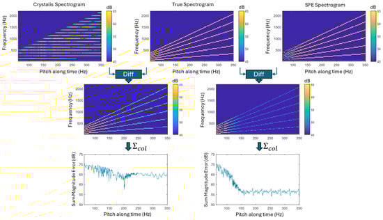
Figure 9.
Comparison of spectrograms generated by Crystalis and SFE against a reference (“true”) spectrogram of a synthetic signal with a time-varying pitch (60–350 Hz) and five harmonics (top row). The second row shows difference spectrograms computed using a frequency-neighborhood-based error metric, where each non-zero point in the true spectrogram is compared within a ±62.5 Hz range—equivalent to one FFT bin in Crystalis. Summed error curves across all six harmonics reveal that SFE achieves accurate pitch resolution above ~120 Hz, while at lower frequencies, overlapping spectral peaks occasionally lead to missed detections. The Crystalis method expresses low-frequency pitch using a reduced energy and number of FFT bins. At higher frequencies, although the number of bins increases, frequency precision is not obtained.
3.2. Crystalis vs. SFE Electrodograms
In this section, electrodograms of a few representative audio signals (a synthetic tone, speech, and music) are presented as illustrative examples to demonstrate the behavior of each strategy. The purple lines overlaid on the spectrograms (see Figure 10, Figure 11, Figure 12 and Figure 13 in the corresponding sub-sections below) represent the electrodograms generated by Crystalis (left column) and SFE (right column). Each line is plotted at the center frequency of the band assigned to the corresponding electrode, and its height is proportional to the amount of pulse charge delivered to the electrode.
3.2.1. Synthetic Signals (Sine Sweeps)
Figure 10 (top row) displays the electrodograms corresponding to the sine wave followed by a complex tone sweep. This figure also illustrates the sound level in each channel, expressed in dB SPL at the input to the compression block, using a color-coded image (middle row) and one-dimensional plots (bottom row).
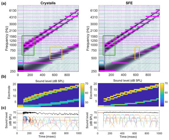
Figure 10.
(a) Electrodograms of Crystalis (left) and SFE (right) for sine (250 Hz, t < 100 msec) and three logarithmic sine sweep waves (250 → 1000; 750 → 5000; 945 → 6300 Hz). The SFE demonstrates improved frequency selectivity (green box), reduced channel interaction (yellow box), and sharper peak selection (blue box). (b,c) Sound level distribution across channels following the N-of-M block. The total input sound level is 70 dB SPL. The distribution of this level at three specific values (67.6, 64.6, and 61.6 dB SPL) is more distinguishable in the SFE compared to Crystalis. In panel (c), the sum of sound levels across channels is shown in black. In this numerical simulation, the pre-accentuation filter was turned off to ensure that a uniform, frequency-independent gain was applied to the signal.
Regarding the initial part of the signal, the 250 Hz sinusoid, the blue rectangle highlights how the spectral content leaks to neighboring electrodes in the Crystalis electrodogram. On the other hand, in SFE, all pulses occur within a single electrode, providing a higher spectral resolution for representing the pure tone.
Looking at the low-frequency component of the complex tone, compared to Crystalis, SFE provides sparser stimulation. The yellow rectangle highlights how the transitions from one electrode channel to the subsequent one happen in a narrower region in SFE than in Crystalis, resulting in a higher resolution representation. There are time intervals in which, for Crystalis, three electrodes are activated at the same frames, while for SFE maximally two adjacent channels would stimulate in the transition bands.
The second and third components of the complex tone sweep are separated in frequency by a factor of 1.26 that corresponds to 4 semi-tones (). The green rectangles highlight how in Crystalis the representation of these two components merge into a larger blurred representation with up to four electrodes being activated at the same time. Conversely, in SFE, each component can be more clearly distinguished. For higher-frequency channels, the resolution diminishes as the filters defined in the FAM are broader.
Regarding the sound level distribution of the input signal across channels, the spectral correction mechanism described in Equation (2)—implemented via the function —and the FSM mechanism together produce a flat trapezoidal sound level distribution at the target levels of 67.6, 64.6, and 61.6 dB SPL, corresponding to the sound pressure level of each sine sweep. This methodology ensures that the input signal’s sound level is accurately preserved when it is presented by a group of spectral peaks, each represented by a sound level at an estimated center frequency.
3.2.2. Speech
The electrodograms for the utterance /abε/ are presented in Figure 11 for both strategies. The key differences are observed in the representation of the vowels. The yellow lines indicate how the formants of the vowels /a/ and /ε/ exhibit an ascending and descending pitch, respectively.
Because SFE enhances the contrast between spectral peaks and valleys compared to Crystalis, the resulting electrodograms are sparser, leading to a more accurate representation of these time-varying formants. The blue rectangles represent the valley areas in which the number of pulses should be minimal. In the SFE, the ascending pitch is clearly observed between 20 ms and 100 ms, where electrodes corresponding to 375, 625, and 875 Hz stop their stimulations around 70 ms. In contrast, Crystalis continues to stimulate these electrodes even when their center frequencies correspond to spectral valleys. A similar situation is observed in the descending pitch of the second vowel between 280 ms and 400 ms.
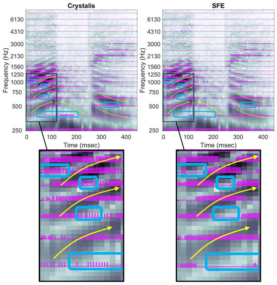
Figure 11.
Electrodograms of Crystalis (left) and SFE (right) for an utterance of the word /abε/. Yellow curves highlight some of the dynamics of the formants and main differences between electrodograms are pointed out by the blue squares. Arrows indicate the variation and placement of the main harmonics, while rectangles highlight the valleys between the principal harmonics where stimulation should drop.
A precise representation of the dynamics of speech formants is particularly important for tonal languages. Figure 12 illustrates the low-frequency region of the electrodograms corresponding to an utterance of the Mandarin syllable /mà/ distinguished by its descending tone. Once again, the SFE electrodogram aligns more closely with the audio spectrogram than the Crystalis electrodogram.
The spectrogram reveals a slight pitch increase around the 6350 ms mark, followed by a more pronounced decrease. In Crystalis, but not in SFE, spurious stimuli appear on the first and second electrodes—around 6350 ms and between 6400 ms—resulting in a poor representation of these dynamics. The variation in the fourth formant, at approximately 700 Hz, is more accurately captured by SFE due to its enhanced frequency resolution.
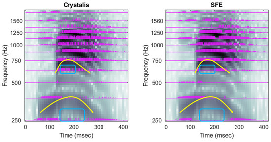
Figure 12.
Electrodograms of Crystalis (left) and SFE (right) for an utterance of the word /mà/. Yellow curves highlight some of the dynamics of the formants and main differences between electrodograms are pointed out by the blue squares. Arrows and rectangles indicate the placement of the main harmonics and the valleys between them.
3.2.3. Music
The next example, depicted in Figure 13, refers to a music extract, the first 3 bars of Beethoven’s Für Elise played on a piano. It can be seen, in the region centered at the 1s mark, that the fundamental component around 650 Hz is more clearly defined in SFE, since the energy leaking to the adjacent electrodes in Crystalis is indisputable. Similarly, the second harmonic around 1300 Hz is clearer in SFE than in Crystalis. Additionally, within this time range, one can notice that SFE manages to provide more information on higher harmonics, in electrode 16 (around 3.9 kHz). This is because in each frame, only a subset of spectral peaks is selected (N-of-M selection). In Crystalis, clusters of adjacent channels are more often selected and do not leave place for higher order harmonics. On the other hand, SFE facilitates the presence of high harmonics in the electrodogram, due to its sparser channel selection. These higher harmonics are useful in distinguishing, at least visually in the figure, the semitone intervals played in this chunk.
Between 1 s and 1.5 s, some note changes, highlighted by green lines, are more evidently portrayed in the SFE electrodogram. One can also identify less spectral leakage to neighboring channels in a more harmonically complex chunk, between 1.5 s and 2 s, when an arpeggio is played.
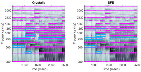
Figure 13.
Electrodograms of Crystalis (left) and SFE (right) for an extract from Beethoven’s Für Elise. Green curves highlight note changes that are more clearly defined in SFE, and spectral leakage is pointed out by the blue squares. The arrow indicates the impact of rapid changes in three consecutive notes on the most energetic part of the spectrum. Rectangles highlight the valleys between the principal harmonics, where stimulation should drop.
3.3. Feature Tracker
In this section, we present the output of the SEE processing for an utterance of the sound /abε/. In this example, the FAM was configured such that, starting from a lower boundary of 80 Hz, the bandwidths of the first six channels increased linearly from 100 Hz to 200 Hz (see Figure 14c). From channel 7 to channel 20, the bandwidths increased logarithmically, distributing the frequency range between the upper boundary of the 6th channel (980 Hz) and the maximum frequency of 7900 Hz equally on a logarithmic scale across the remaining 14 channels.
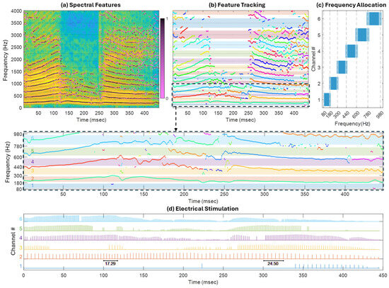
Figure 14.
Illustration of event generation and feature tracking in SEE. (a) spectrogram of the utterance /abε/ with spectral peaks identified during feature extraction. Their respective SFX confidence parameter represented in color scale going from 0 (light pink) to 1 (black); (b) tracked features identified with different colors. The colored patches indicate the passband of trapezoid FSMs for each channel centered around the dashed line, with a magnification of the region comprising channels which use TFS rate coding (1 to 6) below; (c) frequency allocation for channels 1 to 6. The dark blue indicates the passband, and the light blue, the transition regions between consecutive bands; and (d) the corresponding electrical stimulations on channels 1 to 6. To illustrate the variable rate stimulation, the elapsed time between 6 consecutive pulses is shown in the picture for sequences around 100 ms and around 300 ms on channel 2. The electrodogram uses colors matching the passbands shown in (c).
This frequency allocation is arbitrary and is used solely to demonstrate the flexibility of the proposed method in assigning frequency bands to channels. The frequency allocation masks have a trapezoidal shape, where the central plateau represents the passband and the sloped sides define the transition bands.
The maximum stimulation rate was set to 1000 pps. Given that the maximum TFS frequency cannot exceed the stimulation rate, and that the upper boundary of channel 6 is 980 Hz, only the first six channels are capable of conveying TFS information. For the higher-frequency channels, stimulation is performed at a constant rate of 1000 Hz.
Figure 14 illustrates the temporal tracking of spectral features. Panel (a) presents the spectrogram of the utterance /abε/, overlaid with spectral peaks extracted by the SFX event extractor. The confidence level for each detected spectral peak is shown using a color scale ranging from 0 (light pink) to 1 (black). Note that the confidence is close to 1 (i.e., a predominance of black dots) in vowel regions, particularly within the first six formants, which correspond to harmonic sounds. In contrast, lower-confidence peaks are more common during the consonant segment and in higher-frequency formats.
Panel (b) shows how these events are linked over time, enabling the tracking of formant movements. Events that are connected are displayed in the same color and joined by lines. The pastel background colors indicate the frequency bands assigned to each electrode channel. These connections serve as a criterion for selecting between competing events during the channel assignment phase of SEE or for determining which channels to stimulate in each frame within the N-of-M block. A magnified view is provided below panel (b), focusing on the six lowest-frequency channels—those that carry most of the vowel energy and were configured to use TFS time encoding in this example.
Panel (c) displays the frequency allocation for the TFS-coded channels. Dark blue indicates the passband, while light blue represents the transition regions between adjacent bands. Note that the passbands are entirely independent of the FFT bin center frequencies.
Finally, panel (d) shows the resulting electrodogram generated by the SEE strategy, corresponding to the magnified region of the feature tracking. Each channel (electrode) is represented in a different color corresponding to pastel background colors. TFS temporal coding is evident as the stimulation rates increase from channel 1 to channel 6. Moreover, the stimulation rate within each channel is also variable. For example, around the 100 ms mark on channel 2, the total duration of five consecutive stimulation periods is 17.29 ms, corresponding to a stimulation rate of 289 pps. In contrast, around the 300 ms mark, the duration increases to 24.5 ms, corresponding to a reduced rate of 204 pps.
4. Discussion
The SFE coding strategy presented in this article offers FFT-based sound coding with enhanced spectral resolution, even at a fraction of an FFT bin (i.e., sub-bin). The SFE falls under CIS coding strategies that can be easily implemented in CI sound processors without requiring any technological enhancements in the current CI hardware design. Although the SFE is based on Crystalis, other CIS-based coding strategies, such as Advanced Combination Encoder (ACE), can be extended to SFE by substituting their frequency analysis block with the SFX processing block.
Providing frequency resolution at a sub-bin level—enabled by the SFX block—allows for a more flexible clinical FAM that can better align with anatomical tonotopy. In contrast, restricting each electrode’s bandwidth to integer multiples of the FFT bin may lead to discrepancies between clinical and anatomical frequency maps, potentially degrading hearing performance. Creff et al. demonstrated in a study involving 24 CI users that speech recognition in noise was significantly improved with tonotopic fitting across all tested signal-to-noise ratios (0 to 9 dB) [36]. Similarly, a study by Lassaletta et al. showed that anatomically based fitting maps resulted in lower frequency-to-place mismatches compared to default fitting maps. Although the performance improvement with anatomical maps was not statistically significant, most participants (7 out of 8) preferred the anatomical maps over their clinical counterparts [37].
Saadoun et al. demonstrated that word recognition scores can improve—particularly in noisy environments—when the FAM is optimized using an evolutionary algorithm [35]. However, the effectiveness of such algorithms is limited in FFT-based coding strategies (such as ACE and Crystalis) due to constraints requiring bandwidth values to be multiples of the FFT bin size. The SFE addresses this limitation by enabling a flexible FAM, conceptually similar to those used in temporal-based coding strategies like FS4 [38] and HiRes Optima [39]. The enhanced spectral sharpness and improved peak selectivity provided by the SFE improve harmonic distinction, which may support better music appreciation—a common challenge for CI users [40]. Furthermore, the flexible FAM allows for the development of specialized music fitting programs that extend low-frequency coverage, offering additional benefits for CI users [10].
Numerical simulations in our study indicate the enhanced resolution provided by the SFE compared to the reference coding strategy, Crystalis. When processing speech signals, this improved resolution results in a more accurate representation of vowel formant transitions. These transitions—shaped by the consonants preceding and following the vowel—are critical cues for phoneme identification [41]. Consequently, SFE is expected to improve speech recognition for CI recipients.
The numerical simulations also reveal that pitch variations over time are more distinctly represented with SFE. This could be especially beneficial for speech recognition in tonal languages and for music appreciation—two domains where current CI technologies often underperform [42,43]. These benefits could be further enhanced by incorporating temporal fine structure (TFS) information into the electrical stimulation, a feature that could be integrated into the extended SEE strategy, as illustrated in Figure 14.
The results show that the SFE strategy generates sparser electrodograms compared to Crystalis. This increased sparsity may enhance pitch representation by better capturing the dynamic behavior of vowel formants and melodic contours. Additionally, the reduced channel activity in regions corresponding to spectral valleys helps limit the spread of neural excitation within the cochlea. Together, these features highlight the potential of the SFE strategy to improve both speech understanding and music appreciation for cochlear implant users.
Zhang et al. have compared the Crystalis and SFE strategies in an acute clinical study, focusing on two key psychoacoustic aspects: speech recognition and sound quality [31]. Both strategies used similar FAMs due to the acuteness of the clinical evaluation and the inflexible FAM in Crystalis, although the SFE allowed for adjustments to better align with cochlear place frequencies. This design may contribute to faster adaptation in CI users over the short course of evaluation [44].
Regarding speech recognition thresholds, on the first day of testing, the group mean Speech Recognition Threshold (SRT) was better (i.e., lower) with Crystalis (4.4 dB SNR) compared to SFE (7.2 dB SNR) across all six participants. However, by the final testing day (day 3), the group mean SRTs for Crystalis and SFE were identical at 4.0 dB SNR, showing no significant difference. Notably, three participants experienced individual benefits with SFE, achieving improvements of 0.8, 0.7, and 1.7 dB over Crystalis. In other words, despite initial unfamiliarity with the SFE sound, some participants were able to recognize speech in noisy environments at levels comparable to those achieved with Crystalis. Moreover, some CI users—particularly those with better baseline performance—appeared to utilize the spectral cues provided by SFE more effectively after a brief familiarization period.
Regarding sound and music quality, as assessed using the Multiple Stimulus with Hidden Reference and Anchor (MUSHRA) test, results indicated a slight preference for Crystalis over SFE. Interestingly, 2 out of 6 participants preferred the SFE strategy. Authors hypothesized that participants’ familiarity with the Crystalis strategy may have influenced their subjective ratings in its favor. When the MUSHRA test was applied to environmental sounds—where familiarity plays a smaller role—the ratings for SFE showed minimal degradation compared to those for Crystalis. This suggests that the unfamiliarity with SFE’s stimulation pattern may have impacted its perceived quality in the acute setting. Adapting to a new coding strategy can be challenging in short-term evaluations. For example, Roy et al. [45] found that although cochlear implant users initially preferred the CIS strategy over the newer FSP strategy, this preference diminished after one month of FSP use and disappeared entirely after two years. Given the wide variability in musical background and subjective preferences among individuals [46], it is reasonable to conclude that improving perceived sound quality with a novel coding strategy requires a longer adaptation period.
In this article, we demonstrated how the SFE strategy can be extended into the SEE—a novel coding strategy designed to convey TFS information to CI users. To the best of our knowledge, SEE is the first FFT-based coding strategy to integrate temporal cues (i.e., acoustic events) into electrical stimulation. In contrast, existing TFS-based strategies such as FS4 and HiRes rely on temporal filterbanks to achieve this. Therefore, our work lays the groundwork for future clinical studies to compare spectral-based (FFT) and temporal-based (filterbank) approaches to TFS processing.
SEE combines the high spectral resolution provided by the SFX block (i.e., the frequency analyzer in SFE) with the temporal characteristics of the input acoustic signal at each identified spectral peak. Unlike temporal filterbanks, which are not known by their fine spectral selectivity and may include multiple spectral peaks within a single filter’s passband, SEE offers enhanced spectral peak selection precision. This is achieved through a combination of double-FFT analysis, a de-smearing method for peak sharpening, and a trapezoid FSM that further refines peak selection.
However, as with any advancement, high-resolution spectral selectivity comes with trade-offs. One key challenge lies in the temporal tracking of acoustic events. Due to the wideband and nonstationary nature of acoustic signals, adjacent FFT frames may exhibit inconsistent zero-crossing phases. This inconsistency can lead to phase jittering, which undermines the reliability of temporal event extraction.
To address this, the SEE strategy incorporates a feature tracking block that links spectral features across time. This mechanism helps to stabilize phase information by correcting frame-to-frame jitters caused by noise and the inherent properties of FFT-based analysis. In essence, feature tracking enhances the temporal consistency of phase values used to encode temporal events. Based on speech long-term pitch variation rates of up to approximately 300 semitones per second [47], a coding strategy with a stimulation rate of 500 pps (i.e., 2 ms frame duration) would correspond to a pitch change of about 0.6 semitones per frame, or roughly a frequency shift of (calculated as ). However, the presence of noise, asymmetrical spectral peaks, and rapid short-term pitch fluctuations may require increasing this search boundary. Identifying the optimal lower and upper frequency search limits under various noisy conditions could further enhance the robustness and perceptual quality of the SEE strategy and may serve as a direction for future research.
Despite promising numerical simulation results, the clinical performance of the SEE strategy has not yet been evaluated. This is primarily due to technological limitations in Oticon Medical’s Neuro-Zti implants, which are designed for CIS-based strategies. These implants deliver stimulation in a fixed apical-to-basal (or reverse) sequence and cannot accommodate the flexible, event-driven pulse timing required by SEE. As a result, any observed stimulation jitter in current systems may not reflect the true potential of the SEE strategy. To fully realize its benefits, future studies will require implants capable of delivering pulses at arbitrary times, independent of CIS constraints.
In this study, we introduced a confidence parameter for spectral peaks within the SFX block. However, this parameter was not yet utilized in any downstream processing stages. One promising application of this parameter is in evaluating the significance of a stimulation pulse and determining the degree of time jitter it can tolerate in the frame generator block. Spectral peaks with lower confidence values could potentially withstand greater jitter without significantly impacting hearing performance.
This concept could be particularly useful when adapting the SEE strategy for use with older-generation implants that only support CIS-based stimulation. In such cases, the confidence parameter could help prioritize the temporal precision of voiced components—typically associated with higher confidence values—while allowing more jitter in unvoiced, noisier segments, which naturally have lower confidence.
There is also room for further enhancement of the proposed coding strategies. In the current SFE implementation, a 16-millisecond window was used for FFT analysis. This provides a longer window than the one used in Crystalis; therefore, there is a risk that high-frequency components are more blurred in SFE than in Crystalis. Employing wavelet transforms or a combination of multi-length FFT analyzers could improve both temporal and spectral resolution, particularly by optimizing low-frequency and high-frequency channel processing. Additionally, peak selection in the SFX block could be modified to address overlapped peaks at very close center frequencies (e.g., pitch frequencies below ~100 Hz), where overlapping causes peak detection to fail. Lastly, the peak selection methodology may benefit from temporal feedback—using peak locations from previous frames to guide the analysis of the current frame. This would help to maintain feature coherence in noisy environments.
5. Conclusions
The SFE coding strategy offers enhanced spectral peak selectivity and improved spectral sharpness, leading to better harmonic distinction at the level of electrical stimulation for cochlear implant users. Numerical simulations indicate that pitch pursuing in voiced speech segments is more accurate with the SFE strategy, with reduced energy leakage into adjacent channels compared to the Crystalis strategy. A clinical investigation confirmed that SFE is at par with Crystalis in terms of SRT50, even in acute testing conditions. However, acute testing did not show an advantage for SFE in terms of speech recognition and music appreciation. Non-acute testing is needed to identify the underlying cause.
The SEE strategy provides a framework for a temporal fine structure coding approach using FFT-based methods. Numerical simulations demonstrate that features—particularly those related to harmonic sounds—can be tracked across adjacent frames. These tracked features enable more robust detection of zero-crossing events compared to analyzing each frame independently.
6. Patents
Segovia-Martinez Manuel, Felding Skovgaard Julian, Stahl Pierre, Dang Kai, and Wijetillake Aswin. 2023. Cochlear stimulation system with an improved method for determining a temporal fine structure parameter. US Patent US11792578B2, filed 30 July 2019, and issued 17 October 2023.
Author Contributions
Conceptualization, M.S.-M., B.M.-A., J.F. and A.A.W.; methodology, B.M.-A., M.S.-M., J.F., A.A.W., R.A.C. and Y.Z.; software, B.M.-A., R.A.C., J.F. and A.A.W.; validation, B.M.-A., R.A.C., J.F. and A.A.W.; formal analysis, B.M.-A., R.A.C., J.F., A.A.W., Y.Z. and M.S.-M.; investigation, M.S.-M., J.F., B.M.-A. and A.A.W.; resources, M.S.-M. and B.M.-A.; data curation, B.M.-A., R.A.C., Y.Z. and P.T.J.; writing—original draft preparation, B.M.-A., M.S.-M. and R.A.C.; writing—review and editing, All authors; visualization, B.M.-A. and R.A.C.; supervision, M.S.-M. and E.A.L.-P.; project administration, M.S.-M. and E.A.L.-P.; funding acquisition, M.S.-M. All authors have read and agreed to the published version of the manuscript.
Funding
Work funded by Oticon Medical.
Institutional Review Board Statement
Not applicable.
Informed Consent Statement
Not applicable. This study does not report new human experimental data.
Data Availability Statement
The electrodogram data can be requested from the corresponding author.
Conflicts of Interest
B.M.-A., R.A.C., Y.Z., J.F., A.A.W., and M.S.-M. were Oticon Medical employees during this study; B.M.-A., R.A.C., and Y.Z., are now employees of Cochlear Ltd; J.F. and A.A.W., are employees of Demant; P.T.J. and E.A.L.-P. have no conflicts of interest to report.
Abbreviations
The following abbreviations are used in this manuscript:
| ACE | Advanced Combination Encoder |
| CIS | Continuous Interleaved Sampling |
| F2C | Feature to Channel |
| FAM | Frequency Allocation Map |
| FSM | Frequency Selector Mask |
| FSP | Fine Structure Processing |
| E2C | Event to Channel |
| MUSHRA | Multiple Stimulus with Hidden Reference and Anchor |
| SFE | Spectral Feature Extraction |
| SEE | Spectral Event Extraction |
| SRT | Speech Recognition Threshold |
| TFS | Temporal Fine Structure |
Appendix A
Appendix A.1. Crystalis Strategy: A CIS Variant Strategy
This strategy belongs to the family of CIS coding strategies [48,49]. Figure A1 illustrates the main processing blocks within Crystalis. The pre-processing block applies a pre-accentuation 9th order finite impulse response (FIR) filter designed to mimic equal loudness contours in individuals with normal hearing. The frequency content of the pre-accentuated audio signal is subsequently analyzed by an FFT filterbank. To achieve this, the signal is first windowed using an 8-millisecond Hanning window and then its FFT energy spectrum is calculated (i.e., 128-point @ fs = 16,000 Hz, corresponding to an FFT bin size of 125 Hz).
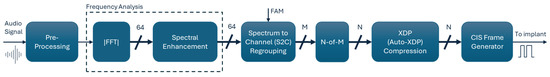
Figure A1.
Signal processing chain for the Crystalis coding strategy.
In the next stage, a spectral enhancement block prunes out any FFT sample that is 7 dB and 45 dB smaller than its adjacent samples and the maximum value of the spectrum, respectively. These two-thresholding address energy smearing and leakage, associated with the main and side lobes of the Hanning window’s frequency response, respectively. The enhanced (i.e., pruned) spectrum is then fed into the spectrum-to-channel regrouping block. This block aggregates FFT bins into M = 20 groups, based on the number of FFT bins assigned to each group as defined in the FAM. The maximum energy value within each group represents the energy of that group.
Usually, a subset of channels with the N ≤ M largest energy values is selected to stimulate their corresponding CI electrodes through the “N-of-M channel selection” block. This block reduces stimulation current interactions between electrodes. The final step in the processing chain involves compressing the selected terms identified by the N-of-M block and mapping them from energy (in dB) to a stimulation duration (in µsec). (Note: For CI devices that use amplitude-modulated stimulations, the output of the compression curve is expressed as stimulation current amplitude instead.)
The eXtended Dynamic Processing (XDP) block provides a compression mapping function for each of the M channels. The compression is either static or may automatically change (i.e., Auto-XDP) its mapping function. This later variant is known as Voice guard commercially. In XDP, each map consists of two piecewise linear functions with a preset connecting kneepoint and two output saturation levels at T- and C-levels. In Auto-XDP the mappings adapt their compression strength by shifting the kneepoint position with the loudness of the input audio signal. In Crystalis, the compression curves are frequency dependent. They are categorized into four groups with similar mapping functions to simplify the fitting procedure of the CI. However, technically, M maps exist in the coding strategy.
Lastly, in the CIS pulse frame generator, the stimulation pulses generated by the compression block in different channels, are concatenated sequentially either from the apical to basal direction or vice versa, to form a packet of stimulation pulses. The packets are transferred to the implant at the requested stimulation rate, measured in pulses per second (pps). The default stimulation rate is 500 pps (corresponding to an FFT hop size of 2 milliseconds). Alternative rates can be achieved by adjusting the analysis rate of the input signal or by dropping, duplicating, or interpolating stimulation packets.
Appendix A.2. Numerical Simulation Parameters
For the numerical simulations in this article, electrodograms were calculated using a stimulation rate of 500 pps and an N-of-M selection of 8 channels. To ensure a fair comparison between the Crystalis and SFE strategies, identical FAMs were used for both. Figure A2 illustrates the frequency response of the analysis filter banks employed in Crystalis and SFE.
Crystalis analysis filters are formed by combining Hanning window spectra centered at different bins of a 128-point FFT, resulting in a rippled frequency response in channels composed of multiple bins. The spectrum enhancement block sets the stopbands of the channels at −7 dB.
Conversely, SFE analysis filters have a trapezoid-like shape, with passband values of 0 dB, crossing points at −3 dB, and stopbands at −6 dB. The passband occupies 75% of the FAM bandwidth. The sum of two adjacent trapezoid FSMs in the transition band equals a gain of 0 dB, ensuring that the total energy of a feature in the transition band remains constant while gradually shifting from one channel to another.
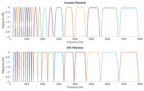
Figure A2.
Filter-banks of Crystalis (top) and SFE (bottom).
Lastly, the XDP compression block was utilized in both Crystalis and SFE strategies to map the input channel energy to output stimulation levels, scaled between the T- and C-levels fixed at 10 and 80 µs, respectively, for all 20 channels. The XDP block parameters were set to the default factory values for a medium-loudness sound environment, as summarized in the table below.

Table A1.
XDP parameter values.
Table A1.
XDP parameter values.
| Frequency Range (Hz) | Electrodes 1 | Knee-Point dB SPL | Knee-Point (C-T)% | Low/Hi IDR dB SPL | T/C-Level µs |
|---|---|---|---|---|---|
| 187.5–1437.5 | E20–E12 | 61 | 70% | 23/95 | 10/80 |
| 1437.5–3437.5 | E11–E6 | 57 | 70% | 23/95 | 10/80 |
| 3437.5–7937.5 | E5–E1 | 50 | 70% | 23/95 | 10/80 |
1 E1 is the first basal electrode.
References
- Wilson, B.S.; Finley, C.C.; Lawson, D.T.; Wolford, R.D.; Zerbi, M. Design and Evaluation of a Continuous Interleaved Sampling (CIS) Processing Strategy for Multichannel Cochlear Implants. J. Rehabil. Res. Dev. 1993, 30, 110–116. [Google Scholar] [PubMed]
- Wilson, B.S.; Finley, C.C.; Lawson, D.T.; Wolford, R.D.; Eddington, D.K.; Rabinowitz, W.M. Better Speech Recognition with Cochlear Implants. Nature 1991, 352, 236–238. [Google Scholar] [CrossRef] [PubMed]
- Carlyon, R.P.; Goehring, T. Cochlear Implant Research and Development in the Twenty-First Century: A Critical Update. J. Assoc. Res. Otolaryngol. 2021, 22, 481–508. [Google Scholar] [CrossRef] [PubMed]
- Henry, F.; Glavin, M.; Jones, E. Noise Reduction in Cochlear Implant Signal Processing: A Review and Recent Developments. IEEE Rev. Biomed. Eng. 2023, 16, 319–331. [Google Scholar] [CrossRef] [PubMed]
- Goupell, M.J. Pushing the Envelope of Auditory Research with Cochlear Implants. Acoust. Today 2015, 11, 26–33. [Google Scholar]
- McDermott, H.J. Music Perception with Cochlear Implants: A Review. Trends Amplif. 2004, 8, 49–82. [Google Scholar] [CrossRef] [PubMed]
- Landsberger, D.M.; Svrakic, M.; Roland, J.T.; Svirsky, M. The Relationship Between Insertion Angles, Default Frequency Allocations, and Spiral Ganglion Place Pitch in Cochlear Implants. Ear Hear. 2015, 36, e207–e213. [Google Scholar] [CrossRef] [PubMed]
- Jiam, N.T.; Gilbert, M.; Cooke, D.; Jiradejvong, P.; Barrett, K.; Caldwell, M.; Limb, C.J. Association Between Flat-Panel Computed Tomographic Imaging–Guided Place-Pitch Mapping and Speech and Pitch Perception in Cochlear Implant Users. JAMA Otolaryngol.-Head Neck Surg. 2019, 145, 109–116. [Google Scholar] [CrossRef] [PubMed]
- Kan, A.; Stoelb, C.; Litovsky, R.Y.; Goupell, M.J. Effect of Mismatched Place-of-Stimulation on Binaural Fusion and Lateralization in Bilateral Cochlear-Implant Users. J. Acoust. Soc. Am. 2013, 134, 2923–2936. [Google Scholar] [CrossRef] [PubMed]
- Nogueira, W.; Nagathil, A.; Martin, R. Making Music More Accessible for Cochlear Implant Listeners: Recent Developments. IEEE Signal Process. Mag. 2019, 36, 115–127. [Google Scholar] [CrossRef]
- Geurts, L.; Wouters, J. Better Place-Coding of the Fundamental Frequency in Cochlear Implants. J. Acoust. Soc. Am. 2004, 115, 844–852. [Google Scholar] [CrossRef] [PubMed]
- Fourakis, M.S.; Hawks, J.W.; Holden, L.K.; Skinner, M.W.; Holden, T.A. Effect of Frequency Boundary Assignment on Vowel Recognition with the Nucleus 24 ACE Speech Coding Strategy. J. Am. Acad. Audiol. 2004, 15, 281–299. [Google Scholar] [CrossRef] [PubMed]
- McKay, C.M.; Henshall, K.R. Frequency-to-Electrode Allocation and Speech Perception with Cochlear Implants. J. Acoust. Soc. Am. 2002, 111, 1036–1044. [Google Scholar] [CrossRef] [PubMed]
- Tabibi, S.; Kegel, A.; Lai, W.K.; Dillier, N. Investigating the Use of a Gammatone Filterbank for a Cochlear Implant Coding Strategy. J. Neurosci. Methods 2017, 277, 63–74. [Google Scholar] [CrossRef] [PubMed]
- Kasturi, K.; Loizou, P.C. Effect of Filter Spacing on Melody Recognition: Acoustic and Electric Hearing. J. Acoust. Soc. Am. 2007, 122, EL29–EL34. [Google Scholar] [CrossRef] [PubMed]
- Omran, S.A.; Lai, W.; Büchler, M.; Dillier, N. Semitone Frequency Mapping to Improve Music Representation for Nucleus Cochlear Implants. EURASIP J. Audio Speech Music Process. 2011, 2011, 2. [Google Scholar] [CrossRef]
- Goehring, T.; Archer-Boyd, A.W.; Arenberg, J.G.; Carlyon, R.P. The Effect of Increased Channel Interaction on Speech Perception with Cochlear Implants. Sci. Rep. 2021, 11, 10383. [Google Scholar] [CrossRef] [PubMed]
- Nogueira, W.; Rode, T.; Büchner, A. Spectral Contrast Enhancement Improves Speech Intelligibility in Noise for Cochlear Implants. J. Acoust. Soc. Am. 2016, 139, 728–739. [Google Scholar] [CrossRef] [PubMed]
- Nogueira, W.; Litvak, L.; Edler, B.; Ostermann, J.; Büchner, A. Signal Processing Strategies for Cochlear Implants Using Current Steering. EURASIP J. Adv. Signal Process. 2009, 2009, 531213. [Google Scholar] [CrossRef]
- Nogueira, W.; Kátai, A.; Harczos, T.; Klefenz, F.; Buechner, A.; Edler, B. An Auditory Model Based Strategy for Cochlear Implants. In Proceedings of the Annual International Conference of the IEEE Engineering in Medicine and Biology-Proceedings, Lyon, France, 22–26 August 2007; pp. 4127–4130. [Google Scholar]
- Stahl, P.; Dang, K.; Vandersteen, C.; Guevara, N.; Clerc, M.; Gnansia, D. Current Distribution of Distributed All-Polar Cochlear Implant Stimulation Mode Measured in-Situ. PLoS ONE 2022, 17, e0275961. [Google Scholar] [CrossRef] [PubMed]
- Lee, S.Y.; Kim, Y.S.; Jo, H.D.; Kim, Y.; Carandang, M.; Huh, G.; Choi, B.Y. Effects of in vivo Repositioning of Slim Modiolar Electrodes on Electrical Thresholds and Speech Perception. Sci. Rep. 2021, 11, 15135. [Google Scholar] [CrossRef] [PubMed]
- Moore, B.C.J. Coding of Sounds in the Auditory System and Its Relevance to Signal Processing and Coding in Cochlear Implants. Otol. Neurotol. 2003, 24, 243–254. [Google Scholar] [CrossRef] [PubMed]
- Li, X.; Nie, K.; Atlas, L.; Rubinstein, J. Harmonic Coherent Demodulation for Improving Sound Coding in Cochlear Implants. In Proceedings of the ICASSP, IEEE International Conference on Acoustics, Speech and Signal Processing, Dallas, TX, USA, 14–19 March 2010; Proceedings. Institute of Electrical and Electronics Engineers Inc.: New York, NY, USA, 2010; pp. 5462–5465. [Google Scholar]
- Zhou, H.; Kan, A.; Yu, G.; Guo, Z.; Zheng, N.; Meng, Q. Pitch Perception with the Temporal Limits Encoder for Cochlear Implants. IEEE Trans. Neural Syst. Rehabil. Eng. 2022, 30, 2528–2539. [Google Scholar] [CrossRef] [PubMed]
- Zierhofer, C.; Schatzer, R. A Fine Structure Stimulation Strategy and Related Concepts. In Cochlear Implant Research Updates; IntechOpen: London, UK, 2012. [Google Scholar]
- Riss, D.; Hamzavi, J.-S.; Selberherr, A.; Kaider, A.; Blineder, M.; Starlinger, V.; Gstoettner, W.; Arnoldner, C. Envelope versus Fine Structure Speech Coding Strategy: A Crossover Study. Otol. Neurotol. 2011, 32, 1094–1101. [Google Scholar] [CrossRef] [PubMed]
- Magnusson, L. Comparison of the Fine Structure Processing (FSP) Strategy and the CIS Strategy Used in the MED-EL Cochlear Implant System: Speech Intelligibility and Music Sound Quality. Int. J. Audiol. 2011, 50, 279–287. [Google Scholar] [CrossRef] [PubMed]
- Riss, D.; Hamzavi, J.-S.; Blineder, M.; Flak, S.; Baumgartner, W.-D.; Kaider, A.; Arnoldner, C. Effects of Stimulation Rate with the FS4 and HDCIS Coding Strategies in Cochlear Implant Recipients. Otol. Neurotol. 2016, 37, 882–888. [Google Scholar] [CrossRef] [PubMed]
- Müller, J.; Brill, S.; Hagen, R.; Moeltner, A.; Brockmeier, S.J.; Stark, T.; Helbig, S.; Maurer, J.; Zahnert, T.; Zierhofer, C.; et al. Clinical Trial Results with the Med-El Fine Structure Processing Coding Strategy in Experienced Cochlear Implant Users. ORL 2012, 74, 185–198. [Google Scholar] [CrossRef] [PubMed]
- Zhang, Y.; Johannesen, P.T.; Molaee-Ardekani, B.; Wijetillake, A.; Attili Chiea, R.; Hasan, P.Y.; Segovia-Martínez, M.; Lopez-Poveda, E.A. Comparison of Performance for Cochlear-Implant Listeners Using Audio Processing Strategies Based on Short-Time Fast Fourier Transform or Spectral Feature Extraction. Ear Hear. 2024, 46, 163–183. [Google Scholar] [CrossRef] [PubMed]
- Bergeron, F.; Hotton, M. Perception in Noise with the Digisonic SP Cochlear Implant: Clinical Trial of Saphyr Processor’s Upgraded Signal Processing. Eur. Ann. Otorhinolaryngol. Head. Neck Dis. 2016, 133, S4–S6. [Google Scholar] [CrossRef] [PubMed]
- Langner, F.; Büchner, A.; Nogueira, W. Evaluation of an Adaptive Dynamic Compensation System in Cochlear Implant Listeners. Trends Hear. 2020, 24. [Google Scholar] [CrossRef] [PubMed]
- Oppenheim, A.V.; Schafer, R.W. Discrete-Time Signal Processing (Prentice-Hall Signal Processing Series), 3rd ed.; Pearson: Bloomington, MN, USA, 2009. [Google Scholar]
- Saadoun, A.; Schein, A.; Péan, V.; Legrand, P.; Aho Glélé, L.S.; Grayeli, A.B. Frequency Fitting Optimization Using Evolutionary Algorithm in Cochlear Implant Users with Bimodal Binaural Hearing. Brain Sci. 2022, 12, 253. [Google Scholar] [CrossRef] [PubMed]
- Creff, G.; Lambert, C.; Coudert, P.; Pean, V.; Laurent, S.; Godey, B. Comparison of Tonotopic and Default Frequency Fitting for Speech Understanding in Noise in New Cochlear Implantees: A Prospective, Randomized, Double-Blind, Cross-Over Study. Ear Hear. 2024, 45, 35–52. [Google Scholar] [CrossRef] [PubMed]
- Lassaletta, L.; Calvino, M.; Sánchez-Cuadrado, I.; Gavilán, J. Does It Make Any Sense to Fit Cochlear Implants According to the Anatomy-Based Fitting? Our Experience with the First Series of Patients. Front. Audiol. Otol. 2023, 1, 1298538. [Google Scholar] [CrossRef]
- Riss, D.; Hamzavi, J.S.; Blineder, M.; Honeder, C.; Ehrenreich, I.; Kaider, A.; Baumgartner, W.D.; Gstoettner, W.; Arnoldner, C. FS4, FS4-p, and FSP: A 4-Month Crossover Study of 3 Fine Structure Sound-Coding Strategies. Ear Hear. 2014, 35, e272–e281. [Google Scholar] [CrossRef] [PubMed]
- Firszt, J.B.; Holden, L.K.; Reeder, R.M.; Skinner, M.W. Speech Recognition in Cochlear Implant Recipients: Comparison of Standard HiRes and HiRes 120 Sound Processing. Otol. Neurotol. 2009, 30, 146–152. [Google Scholar] [CrossRef] [PubMed]
- Tahmasebi, S.; Segovia-Martinez, M.; Nogueira, W. Optimization of Sound Coding Strategies to Make Singing Music More Accessible for Cochlear Implant Users. Trends Hear. 2023, 27, 23312165221148022. [Google Scholar] [CrossRef] [PubMed]
- Hillenbrand, J.M.; Clark, M.J.; Nearey, T.M. Effects of Consonant Environment on Vowel Formant Patterns. J. Acoust. Soc. Am. 2001, 109, 748–763. [Google Scholar] [CrossRef] [PubMed]
- Bleckly, F.; Lo, C.Y.; Rapport, F.; Clay-Williams, R. Music Perception, Appreciation, and Participation in Postlingually Deafened Adults and Cochlear Implant Users: A Systematic Literature Review. Trends Hear. 2024, 28, 23312165241287391. [Google Scholar] [CrossRef] [PubMed]
- Liu, H.; Peng, X.; Zhao, Y.; Ni, X. The Effectiveness of Sound-Processing Strategies on Tonal Language Cochlear Implant Users: A Systematic Review. Pediatr. Investig. 2017, 1, 32–39. [Google Scholar] [CrossRef] [PubMed]
- Di Maro, F.; Carner, M.; Sacchetto, A.; Soloperto, D.; Marchioni, D. Frequency Reallocation Based on Cochlear Place Frequencies in Cochlear Implants: A Pilot Study. Eur. Arch. Oto-Rhino-Laryngol. 2022, 279, 4719–4725. [Google Scholar] [CrossRef] [PubMed]
- Roy, A.T.; Carver, C.; Jiradejvong, P.; Limb, C.J. Musical Sound Quality in Cochlear Implant Users: A Comparison in Bass Frequency Perception between Fine Structure Processing and High-Definition Continuous Interleaved Sampling Strategies. Ear Hear. 2015, 36, 582–590. [Google Scholar] [CrossRef] [PubMed]
- Gfeller, K.; Oleson, J.; Knutson, J.F.; Breheny, P.; Driscoll, V.; Olszewski, C. Multivariate Predictors of Music Perception and Appraisal by Adult Cochlear Implant Users. J. Am. Acad. Audiol. 2008, 19, 120–134. [Google Scholar] [CrossRef] [PubMed]
- Xu, Y.; Sun, X. Maximum Speed of Pitch Change and How It May Relate to Speech. J. Acoust. Soc. Am. 2002, 111, 1399–1413. [Google Scholar] [CrossRef] [PubMed]
- Zeng, F. Trends in Cochlear Implants. Trends Amplif. 2004, 8, 1–34. [Google Scholar] [CrossRef] [PubMed]
- Kiefer, J.; Hohl, S.; Stürzebecher, E.; Pfennigdorff, T.; Gstöettner, W. Comparison of Speech Recognition with Different Speech Coding Strategies (SPEAK, CIS, and ACE) and Their Relationship to Telemetric Measures of Compound Action Potentials in the Nucleus CI 24M Cochlear Implant System. Audiology 2001, 40, 32–42. [Google Scholar] [CrossRef] [PubMed]
Disclaimer/Publisher’s Note: The statements, opinions and data contained in all publications are solely those of the individual author(s) and contributor(s) and not of MDPI and/or the editor(s). MDPI and/or the editor(s) disclaim responsibility for any injury to people or property resulting from any ideas, methods, instructions or products referred to in the content. |
© 2025 by the authors. Licensee MDPI, Basel, Switzerland. This article is an open access article distributed under the terms and conditions of the Creative Commons Attribution (CC BY) license (https://creativecommons.org/licenses/by/4.0/).