A Systematic Approach for Robotic System Development

Abstract

This paper introduces a unified and systematic design methodology for robotic systems that is generalizable across a wide range of applications. It integrates rigorous mathematical formalisms such as kinematics, dynamics, control theory, and optimization with advanced simulation tools, ensuring that each design decision is grounded in provable theory. The approach defines clear phases, including mathematical modeling, virtual prototyping, parameter optimization, and theoretical validation. Each phase builds on the previous one to reduce unforeseen integration issues. Spanning from conceptualization to deployment, it offers a blueprint for developing mathematically valid and robust robotic solutions while streamlining the transition from design intent to functional prototype. By standardizing the design workflow, this framework reduces development time and cost, improves reproducibility across projects, and enhances collaboration among multidisciplinary teams. Such a generalized approach is essential in today’s fast-evolving robotics landscape where rapid innovation and cross-domain applicability demand flexible yet reliable methodologies. Moreover, it provides a common language and set of benchmarks that both novice and experienced engineers can use to evaluate performance, facilitate knowledge transfer, and future-proof systems against emerging application requirements.

1. Introduction

The evolution of robotics in recent decades has led to the development of increasingly complex, versatile, and interconnected systems. This progress has necessitated a shift from ad hoc experimental approaches to rigorous design and verification methodologies, based on solid mathematical foundations [1]. The adoption of formal methods allows for precise behavior prediction, performance optimization, and reduced development costs [1,2].

Modern robots combine mechanics, electronics, computer science, and control theory, requiring integrated multidisciplinary mathematical modeling that links theoretical design to practical implementation [3]. A robust mathematical framework, as emphasized by Murray et al. [4], is essential to define reliable control architectures, optimize performance, and ensure accurate prediction of system behavior. However, despite significant advances, robotic system modeling continues to present open challenges. The increase in subsystems, dynamic environments, and physical limitations requires standardized techniques that guarantee reliability, security, and scalability [2,5]. Key challenges include modeling environmental interaction, uncertainty management, multirobot adaptability, actuator saturation, and computational limitations [5]. In addition, the resilience of robotic systems in uncertain environments is an increasingly important dimension. Applications such as tunneling robotics demonstrate the need for design solutions that take into account changing environmental factors and structural reliability [6]. Integrating resiliency into the design not only increases the robustness of the system but also allows it to cope with dynamic environments with greater adaptability. In this context, an approach to modeling based on solid theoretical principles and open to integration with emerging paradigms is the key to addressing the challenges of modern robotic systems. In response to these challenges, the increasing availability of sensory data and the computational power available today pave the way for the development hybrid models, in which a priori knowledge is integrated with empirical information [7,8].

Kinematic modeling represents the first abstraction level that describes geometric relationships between robot components and forms the basis for dynamic analysis and control. The Denavit–Hartenberg (DH) [9] formalism enables systematic representation of serial manipulators through homogeneous transformation matrices with reduced parameters, standardized by Craig [10]. The problem of inverse kinematics presents an even more complex challenge. Although analytical solutions are available for simple configurations, robots with more complex structures require the adoption of iterative numerical methods [1]. Alternative approaches based on neural networks [11] and genetic algorithms [12] have also been proposed, effective even in the presence of singular configurations.

Dynamic modeling represents the next abstraction level, fundamental to understanding how forces affect robot motion. The Lagrangian formalism is particularly useful for deriving motion equations in complex systems, with Featherstone [13] proposing efficient algorithms that reduce computational complexity. A critical element in this phase is the identification of the physical parameters of the system. Khalil and Dombre [14] defined systematic procedures for parametric identification, combining analytical models and experimental data. The accuracy of these parameters directly affects the fidelity of the dynamic model and the effectiveness of the control.

Once the equations of motion have been defined and the physical parameters have been estimated, we proceed with the synthesis of the control, a phase in which the model is used to derive effective operating laws, aimed at regulating the behavior of the system, to complete the modeling process. The initial schemes, based on PID regulators applied to individual joints, have been progressively overcome by nonlinear controllers capable of managing dynamic coupling and structural uncertainties [15]. Lopez et al. [16] introduced robust and adaptive controllers that can address parametric variations and external disturbances, improving system resilience.

Numerical simulation is an essential tool to verify and optimize the theoretical behavior of the robotic system in a controlled virtual environment. As highlighted by Corke [17], these tools allow one to validate modeling hypotheses, optimize design parameters, and test control strategies before their real implementation. The adoption of standardized platforms such as ROS (Robot Operating System), advanced simulation environments such as MATLAB/Simulink, and specialized software such as Adams and ANSYS has significantly simplified the integration between modeling, simulation, and experimentation, standardizing the entire development process [18,19]. The use of open-source tools like ROS also promotes reproducibility by enabling shared benchmarks, modular code bases, and common interfaces. Furthermore, simulation-based workflows and shared models enhance collaboration between researchers and developers, allowing systematic comparison of results and reuse of validated components.

If, on the one hand, numerical simulation supports the integration between modeling and experimentation, on the other hand, the evolution of contemporary robotics introduces challenges that impose an extension of classical modeling paradigms. Collaborative robots, for example, require modeling that includes safe interaction dynamics with humans, while soft robotics, characterized by flexible structures and continuous degrees of freedom, requires tools derived from continuum mechanics [20]. In parallel, machine learning, in particular reinforcement learning [8], is emerging as a complementary approach to physical modeling. Nguyen-Tuong and Peters [21] emphasize the importance of combining data-driven models with analytical models to exploit the strengths of both paradigms, with a view to adaptive and robust modeling. This approach is fully consistent with the proposed method, where reinforcement learning is not an alternative but rather a tool that helps to make design more adaptable in uncertain or poorly defined contexts.

In light of the challenges that have emerged, an integrated methodological framework is proposed for robotic system design, harmonizing consolidated methodologies with emerging techniques through sequential phases: functional specifications, kinematic and dynamic modeling, control synthesis, simulation, optimization, and experimental verification. The approach gradually introduces complexity, uses simulation systematically, and strongly integrates mathematical models with physical implementation.

2. Methodological Framework for Robotic System Design

The design of innovative robotic systems requires a systematic approach that integrates technical, economic, environmental, and ergonomic constraints. The proposed methodology consists of six sequential steps supported by mathematical modeling, numerical simulation, and optimization methods, providing a structured pathway from concept to implementation and ensuring both theoretical rigor and practical applicability across diverse robotic applications.

2.1. Product Design Specification (PDS)

The methodology begins with a critical analysis of the state-of-the-art, including scientific literature, patents, and existing technologies, with the aim of identifying current solutions, unsolved problems, and recurring kinematic and dynamic models, thus providing the basis for subsequent parametric modeling. In parallel, competitive benchmarking is conducted through an analytical and comparative evaluation of competing solutions [22,23]. Subsequently, the Product Design Specifications (PDS) are defined, outlining the project’s methodological approach, identifying functional, performance, regulatory, and environmental requirements based on preliminary analyses, compliance requirements, end-user needs, and expected operating conditions.

The PDS matrix, developed in this phase, provides a structured summary of the design requirements that emerged, gathering key parameters related to kinematics (degrees of freedom and working area), dynamics (maximum velocities and accelerations, required forces and torques), dimensional constraints (geometry, mass, weight distribution), and considerations regarding energy efficiency, sustainability, and infrastructure compatibility. This tool helps guide design decisions, allowing the early identification of potential problems and ensuring that the project meets established objectives [24].

The methodology ensures the transferability of the PDS across heterogeneous application areas thanks to the adoption of modular and parametric specifications, which allow for the adaptation and balancing of requirements based on the context. The use of multicriteria decision-making methods with variable weights and trade-off analyses allows for the effective management of conflicting objectives (such as weight/payload optimization), facilitating extensibility across different robotics sectors while ensuring design consistency.

In support of this approach,

Table 1. Example of a Product Design Specification (PDS) to illustrate how it is filled out.

FUNCTION	Example of Product’s Main Function
DIMENSIONS	DIMENSIONAL DATA
	Length	e.g., <50 cm
	Width	e.g., <15 cm
	Weight	e.g., <2 kg
	ACTUATION SYSTEM
	Actuator type	e.g., electric motors, flexible actuators
OPERATIONS	POSITIONING
	Method	e.g., manual or automatic
	CONTROL
	Mode	e.g., microcontroller, user interface
	ADAPTABILITY
	Adjustability	e.g., for variable users or conditions
CONDITIONS OF USE	OPERATING TEMPERATURE
	Operating range	e.g., −10 °C to +60 °C
	EXTERNAL CONDITIONS
	Requirements	e.g., indoor use, dust/water resistant
MANUFACTURING	MANUFACTURING PROCESS
	Technique	e.g., 3D printing, injection molding
MATERIALS	MATERIAL SELECTION
	Type	e.g., plastic, metal, elastomers

presents an example of PDS compilation, highlighting how the modular and flexible structure allows us to adapt the specifications to different robotic fields. This promotes coherence of design choices even in the presence of different regulatory, functional, or performance constraints, contributing to the reusability and scalability of the design process.

2.2. Concept Generation and Evaluation

The next methodological step involves the conceptual design of the robotic system, using structured and creative techniques (brainstorming, morphological diagrams, TRIZ) to generate alternative designs [25]. The generated concepts are verified through direct comparison with the PDS requirements, identifying any inconsistencies and allowing a preliminary selection based on compatibility with the project objectives.

The technical evaluation of concepts is carried out using both qualitative and quantitative methodologies. Within the qualitative framework, the Datum Method enables systematic comparison between alternatives and an ideal or reference baseline, emphasizing relative advantages and identifying potential shortcomings [26]. In parallel, multicriteria quantitative decision-making methods are implemented, using weighted assignment to individual design criteria. These processes enable the computation of composite scores among varying conceptual arrangements, facilitating objective comparison and selection of the optimal concept according to priority specifications established in the PDS [27].

This formalized approach, based on the traceability of design decisions, ensures the identification of the optimal conceptual solution consistent with the stated requirements while establishing a solid foundation for the subsequent detailed design and development phases of the robotic system.

2.3. Simplified Mathematical Modeling

After identifying the optimal concept, the process moves to simplified modeling, which includes an initial technical assessment and the development of a mathematical model based on mechanical principles. Kinematic chains are described using homogeneous transformation matrices to verify mobility and reachability. The dynamics of the multibody system is modeled using Lagrangian or Newton–Euler formulations [28], while modal analysis is used to identify critical frequencies of the system.

The mathematical formulations are solved and implemented using specialized computational tools, chosen based on the type and complexity of the analysis, to support both symbolic and numerical models. MATLAB/Simulink is used for the development and optimization of control algorithms, while ROS-Gazebo enables integrated real-time testing of perception, actuation, and control. Adams supports high-fidelity multibody dynamics simulations, and ANSYS supports structural finite element analysis. The combined use of these tools ensures targeted and effective simulations at every stage of the project [28].

2.4. Parametric CAD Model Development

The selected concept is transferred to a CAD environment, where a solid model and virtual assembly of the entire system are developed (Figure 1). This phase encompasses material and actuator selection, specification of mechanical and electronic interfaces, and application of parametric constraints to enable future optimizations. The parametric CAD environment, coupled with mathematical models, enables automated variant creation and scenario exploration after specification modifications [29].

The integration of advanced tools, such as symbolic solvers, parametric CAD, and real-time simulators (e.g., ROS-Gazebo, MATLAB/Simulink, Adams), enables progressive concept validation through virtual prototyping, overcoming the limitations of traditional design and physical testing alone. This approach ensures an efficient transition to detailed engineering and physical prototyping, ensuring consistency with initial requirements.

2.5. Physical Prototyping

The transition from a theoretical model to a physical system is achieved through the physical prototyping phase. The prototypes are constructed on the basis of previously validated specifications, incorporating mechanical structure, actuation and sensor solutions, and control environment. Implementation often utilizes middleware frameworks such as ROS to ensure modularity and interoperability.

Prototypes may be exploratory, designed to test specific functionalities, or integrated for comprehensive validation. Among the most recent contributions to this phase are rapid manufacturing technologies, such as 3D printing, which significantly reduce development time and enable flexible iteration. These tools represent a clear evolution beyond traditional prototyping, integrating digital modeling with physical realization in a seamless workflow.

This phase represents a critical validation point, where theoretical predictions are confronted with physical reality.

2.6. Experimental Validation

Finally, experimental validation allows us to verify the prototype’s performance under real-world operating conditions through the statistical analysis of collected data and comparison with simulation results, in order to assess the accuracy of theoretical models. In the presence of significant discrepancies, the design is updated through parameter estimation, initiating an iterative refinement cycle. In fact, if the prototype does not meet the performance or regulatory requirements established in the PDS, the process reverts to the previous phases in a continuous flow based on the integration of modeling, simulation, and experimental testing.

This approach ensures the reliability of the design due to the synergy between theory, computational verification, and experimental validation, which constitute the core of the proposed framework, is compatible with different types of robots, and expandable through the integration of digital twins and artificial intelligence techniques [30].

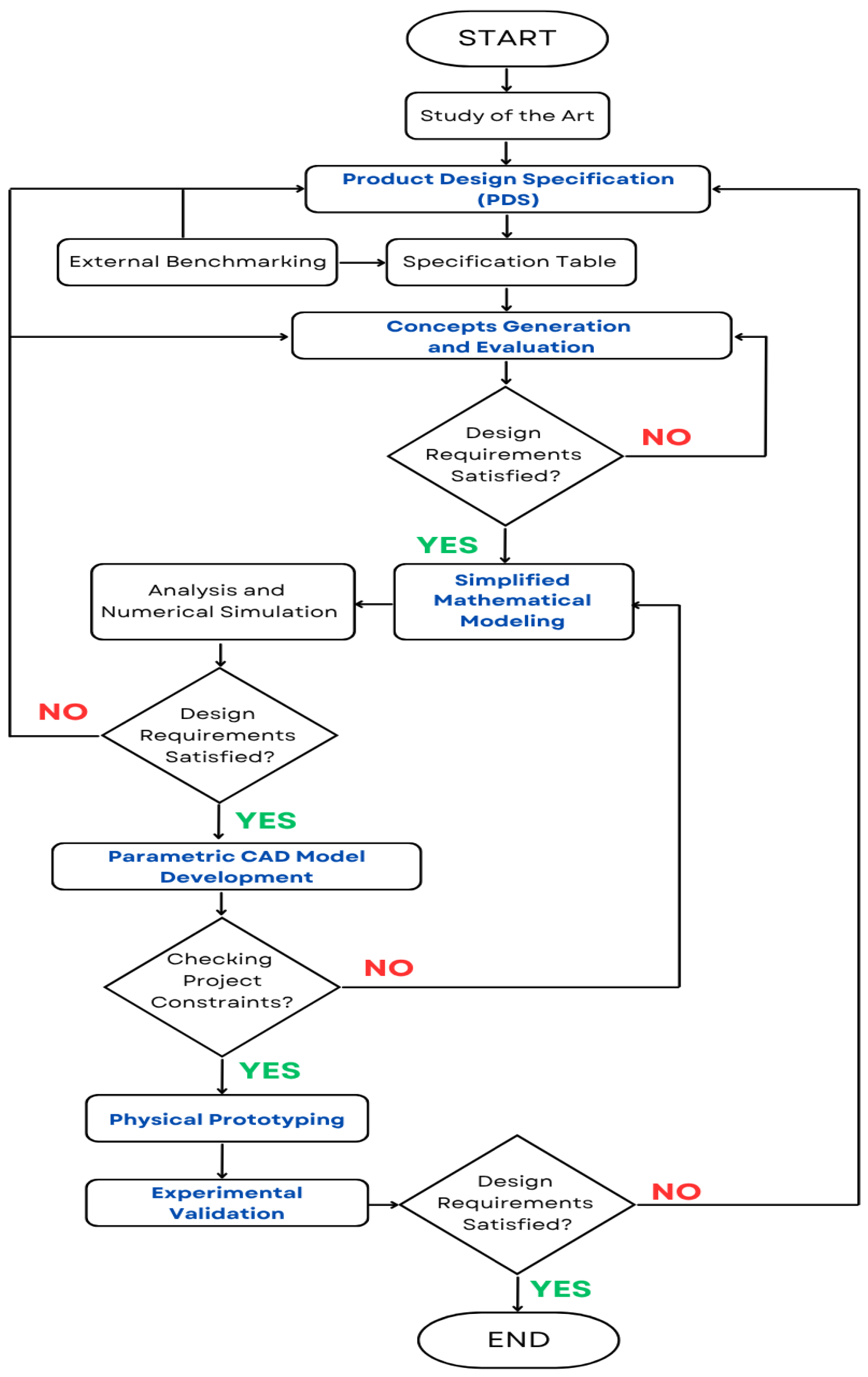
Figure 2 presents the proposed methodological framework, structured as a sequence of iterative phases that integrate conceptual design, modeling, prototyping, and experimental validation, with the innovative elements, highlighted in blue, guiding the process toward a more agile, digitally connected, and data-driven approach.

3. Mathematical Modeling in the Design of Robotic Systems

Mathematical modeling provides the scientific foundation for analyzing, designing, and controlling complex robot systems through formal language and numerical tools. These models systematically relate control variables (joint angles, velocities, torques) to operational space parameters (end-effector position, robot trajectory), supporting motion planning, simulation, optimization, and real-time control [31].

Together, mathematical modeling techniques are an enabler for integrated mechatronic design and for the realization of increasingly efficient, adaptive, and autonomous robots. The interaction between kinematic and dynamic models provides the theoretical basis for a deep understanding of the behavioral properties of robotic systems and facilitates the development from conceptual design to operational realization.

3.1. Kinematic Modeling

Kinematic modeling is of strategic importance from the early design stages up to real-time control of the robotic system, as it describes the geometric relationships between joint parameters and the pose or velocities of the end-effector, excluding the forces responsible for the movement. It is divided into three fundamental components, each of which provides an essential building block for the entire planning, simulation, and control process [1,4].

Direct kinematics analysis determines the end-effector spatial configuration (operational space) from known joint variables (joint space), which are essential for movement simulation and trajectory validation.

The Denavit–Hartenberg (DH) convention systematically describes manipulator geometry [9], representing each joint i with four parameters:

• $a_i$: the distance along the $x_{i-1}$ axis,
• ${\alpha }_i$: the angle of rotation about the $x_{i-1}$ axis,
• $d_i$: the distance along the $z_i$ axis,
• ${\theta }_i$: the angle of rotation about the $z_i$ axis.

The use of these parameters allows for the construction of homogeneous transformation matrices associated with each joint, such as:

$$A_i=\left[\begin{array}{cccc}cos{\theta }_i& -sin{\theta }_{i}cos{\alpha }_i& sin{\theta }_{i}sin{\alpha }_i& a_{i}cos{\theta }_i\\ sin{\theta }_i& cos{\theta }_{i}cos{\alpha }_i& -cos{\theta }_{i}sin{\alpha }_i& a_{i}sin{\theta }_i\\ 0& sin{\alpha }_i& cos{\alpha }_i& d_i\\ 0& 0& 0& 1\end{array}\right]$$

(1)

By sequentially multiplying these transformation matrices, the overall transformation from the robot base to the end effector can be obtained:

$$T_n^0=A_1{A}_2\cdots A_n$$

(2)

Having obtained the overall pose matrix $T_n^0$, it is possible to extract the rotation matrix $R_n^0\in \mathrm{SO}\left(3\right)$ and the translation vector $p_n^0\in {\mathbb{R}}^3$.

After the derivation of the forward kinematics, the inverse kinematics analysis is performed. This involves finding joint variables ${\theta }_i$ or $d_i$ (based on the joint) that allow the end effector to achieve a given spatial posture [1] and is presented as:

$$T_n^0=A_1{A}_2\cdots A_n=T_d$$

(3)

where $T_d$ is the homogeneous target transformation matrix that contains in it the required position and orientation of the end-effector with respect to the reference frame base.

The inverse kinematics problem can be stated as finding the solution of the system of nonlinear equations that results from the equation:

$$T_n^0(\theta ,d)=T_d$$

(4)

where the variables $\theta =[{\theta }_1,{\theta }_2,\dots ,{\theta }_n]$ and $d=[d_1,d_2,\dots ,d_n]$ are the variables to be found. Where possible, an analytical solution uses the geometric constraints of the robot structure to solve the joint variables. Alternatively, iterative numerical methods can be applied, such as Jacobian-based methods, characterized by the following:

$$J\left(q\right)={\displaystyle \frac{\partial x}{\partial q}}\in {\mathbb{R}}^{m\times n}$$

(5)

where x is the vector of position and orientation of the end-effector, derived from the matrix $T_n^0$, m is the size of the operating space (typically 6 for position and orientation), and n is the number of joints of the device being analyzed.

Differential kinematics describes the relationship between joint velocities and end-effector velocities in operational space, essential for motion analysis, singularity handling, and real-time control [31]. This relationship is mediated by the Jacobian matrix, introduced earlier, and expressed as follows:

$$\dot{x}=J\left(q\right)\dot{q}$$

(6)

where:

• $\dot{x}\in {\mathbb{R}}^m$ is the velocity vector in the operational space (typically $m=6$, with 3 components of linear velocity and 3 of angular velocity);
• $\dot{q}\in {\mathbb{R}}^n$ is the vector of joint velocities.

The Jacobian matrix is also essential in the study of kinematic singularity, that is, those that cause the manipulator to lose one or more degrees of freedom and, thus, have unachievable movements. Mathematically, such a condition occurs when:

$$rank\left(J\right)<min(n,m)\Rightarrow det\left(J\right)=0$$

(7)

Figure 3 shows the motion of a 4-DoF manipulator in two configurations: normal (Figure 3a) and singularity (Figure 3b). In the normal configuration, the angles between the segments are non-zero, allowing motion in multiple directions and ensuring a full-rank Jacobian matrix, and thus full control of the end effector. In the singularity configuration, the manipulator is aligned, causing a loss of rank in the Jacobian and, therefore, the inability to generate motion in directions perpendicular to the arm axis. This condition degrades kinematic performance, with consequences for control and motion planning.

The choice of a 4-DoF manipulator stems from the need to clearly represent singularity conditions with a sufficiently complex yet analytically manageable model, effectively illustrating the rank loss of the Jacobian matrix and its impact on the differential control of the final effector. However, the results can be generalized to manipulators with higher DoFs, where singularities also manifest as rank losses, albeit with different implications: in redundant systems ($DoF\ge 6$), rank loss does not exclude the desired motion of the effector, but it can reduce the space of feasible solutions or introduce ambiguity in the inverse kinematic problem. The analysis of the rank, structure, and singular values of the Jacobian matrix therefore remains fundamental to understanding the motion and force capabilities, even in the presence of high redundancy.

The integration of these three analyses supports the entire lifecycle of the robotic system, ensuring accurate modeling, consistent simulation, and reliable execution in complex operating environments. The described kinematic approach applies primarily to open-chain and rigid-body manipulators, while flexible structures, closed chains, or mobile bases require specific methodologies.

3.2. Dynamic Modelling

Dynamic modeling enables high-level robot control by simulating behavior under forces and torques. Unlike kinematics, which addresses geometric aspects, dynamics considers motion causality through forces and torques, proving indispensable for force control, realistic motion simulation, and energy optimization [31].

The dynamic model of the robotic manipulator is often established through analytical representations of the classical mechanics equations. The two most used techniques to obtain the dynamic model are as follows:

• The Newton–Euler formalism, which is based on a recursive process on the force and torque equilibrium that affects each rigid body in the kinematic chain;
• The Lagrangian formalism, wherein the system is based on kinetic and potential energy to reach scalar equations in a compact form.

A classical dynamic equation with a Lagrangian basis is of the type:

$$M\left(q\right)\ddot{q}+C(q,\dot{q})\dot{q}+g\left(q\right)+F\left(\dot{q}\right)=\tau$$

(8)

where:

• $\mathbf{q}\in {\mathbb{R}}^n$: vector of joint variables (joint positions);
• $\dot{\mathbf{q}},\ddot{\mathbf{q}}$: vectors of joint velocity and acceleration;
• $\mathbf{M}\left(\mathbf{q}\right)\in {\mathbb{R}}^{n\times n}$: mass (inertia) matrix of the robot;
• $\mathbf{C}(\mathbf{q},\dot{\mathbf{q}})\dot{\mathbf{q}}$: centripetal and Coriolis term;
• $\mathbf{g}\left(\mathbf{q}\right)$: vector of gravitational forces;
• $\mathbf{F}\left(\dot{\mathbf{q}}\right)$: dissipative term (viscous or Coulomb friction);
• $\tau \in {\mathbb{R}}^n$: vector of actuation torques or forces.

This equation forms the basis of numerous control algorithms, such as inverse dynamic control (computed torque control) or model predictive controllers. Its utilization allows compensation of the robot’s nonlinear dynamics, significantly improving tracking performance, stability, and system responsiveness.

The determination of $\mathbf{M}\left(\mathbf{q}\right)$, $\mathbf{C}(\mathbf{q},\dot{\mathbf{q}})$, and $\mathbf{g}\left(\mathbf{q}\right)$ can be achieved symbolically using multibody modeling tools or through automatic modeling software packages (for example, SymPyBotics, MATLAB Robotics Toolbox). A crucial aspect of dynamic modeling is the precise identification of physical parameters, in particular the dissipative terms $\mathbf{F}\left(\dot{\mathbf{q}}\right)$ that represent friction. Khalil and Dombre [14] have defined rigorous procedures for the parametric identification of industrial robots through analytical and experimental formulations. For nonlinear friction, persistent excitation trajectories with a large spectral richness are used to ensure identifiability. The standard model includes viscous and Coulomb friction, $F\left(\dot{q}\right)=F_c·\mathrm{sign}\left(\dot{q}\right)+F_v\dot{q}$, with parameters estimated by regression on experimental torque and velocity data. For greater fidelity, Stribeck friction models are adopted, with parameters obtained through nonlinear optimization. Cross-validation in independent trajectories generally ensures errors of less than 5% in industrial robots under nominal conditions, directly impacting model accuracy and control effectiveness.

Dynamic modeling, combined with kinematics, enables actuator-compatible trajectories and the simulation of complex scenarios, supporting the design of precise, stable, and flexible robots for advanced automation and improved human–machine interaction.

4. Numerical Simulations for Robotic System Optimization

Following 3D CAD modeling (SolidWorks, Autodesk Inventor, CATIA), we move on to numerical simulation, useful for validating and optimizing system performance. This phase addresses key issues and verifies the robot’s behavior under virtual operating conditions, reducing prototyping costs and times.

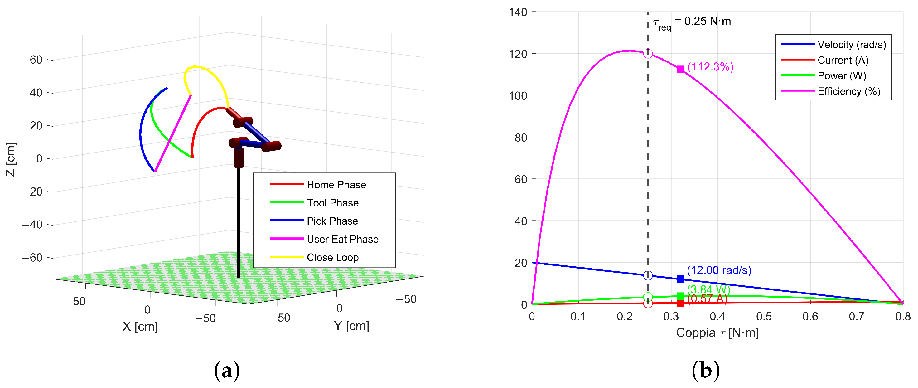
Kinematic simulations verify the geometry and mechanical configuration, analyzing DoF of the system, the path of the elements, the velocities, and the accelerations. Tools such as MATLAB/Simulink, Adams, or CAD motion modules verify the compatibility of the kinematic constraint and the compliance of the motion profile with functional requirements (Figure 4a). Dynamic analyses then incorporate mass effects, forces, inertia, and friction. The simulations allow us to quantify the stresses in the structural components of the robot and the torques/forces applied to the actuators (Figure 4b).

Based on these preliminary results, the device is optimized through multiobjective simulations with geometric parameters, material, control techniques, and actuation configurations. Deterministic and evolutionary optimization algorithms are used to improve parameters such as reducing masses (Figure 5a), maximizing stiffness, optimizing energy consumption, and maximizing positional precision [32]. In the meantime, FEM simulations can be performed to investigate the structural response of the system under static and dynamic loads to avoid failures or undesirable deformation (Figure 5b). This analysis is particularly important at the material selection stage and in sizing of the load members.

Finally, validation of models through integrated simulations allows verification of consistency between the control, electrical, and mechanical subsystems. Within software platforms such as ROS (Robot Operating System) or Gazebo, it is also possible to run simulations by co-simulating the robot’s action under multivariable circumstances, for example, interaction with the environment, obstacles, and moving targets.

5. Control Architectures of a Robotic System

In the design of robotic systems, hierarchical model-based control architectures ensure accuracy of trajectory tracking, robustness to disturbances, and flexibility in handling uncertainties [1,2]. The structure comprises three levels (low, medium, high) with specific complementary functions, as shown in Figure 6.

Experimental validation demonstrates significant improvements over conventional approaches: 45% better tracking accuracy [33], maximum errors of $2.593\times {10}^{-3}$ rad [34], sub-20 ms synchronization latency [35], and 100% constraint enforcement accuracy [36]. Multiplatform statistical analysis confirms significant advantages (p < 0.001) in tracking precision, disturbance rejection, and fault tolerance.

5.1. Low-Level Control

Low-level control executes motion commands precisely by considering nonlinear dynamics and ensuring proper trajectory execution. Various strategies offer specific advantages depending on precision, computational efficiency, and robustness requirements.

One of the most established techniques is Computed Torque Control, a nonlinear inverse control technique [2] using the robot’s full dynamic model for system linearization and decoupling, widely applied in high-precision surgical robotics, industrial assembly, and rehabilitation devices. The control law is defined as:

$$\tau =M\left(q\right)\left({\ddot{q}}_d+K_D({\dot{q}}_d-\dot{q})+K_P(q_d-q)\right)+C(q,\dot{q})\dot{q}+g\left(q\right)$$

(9)

where $q_d,{\dot{q}}_d,{\ddot{q}}_d$ represent the desired trajectories of position, velocity, and acceleration, respectively; $M\left(q\right)$ is the inertia matrix; $C(q,\dot{q})$ represents the Coriolis and centripetal terms; and $g\left(q\right)$ is the gravitational force. The gains $K_P$ and $K_D$ determine the dynamic behavior of the tracking error. This approach is effective for submillimeter accuracy applications, such as computer-assisted surgery (Figure 14f) or rehabilitation devices (Figure 14a,d), where the computational overhead is justified by superior performance.

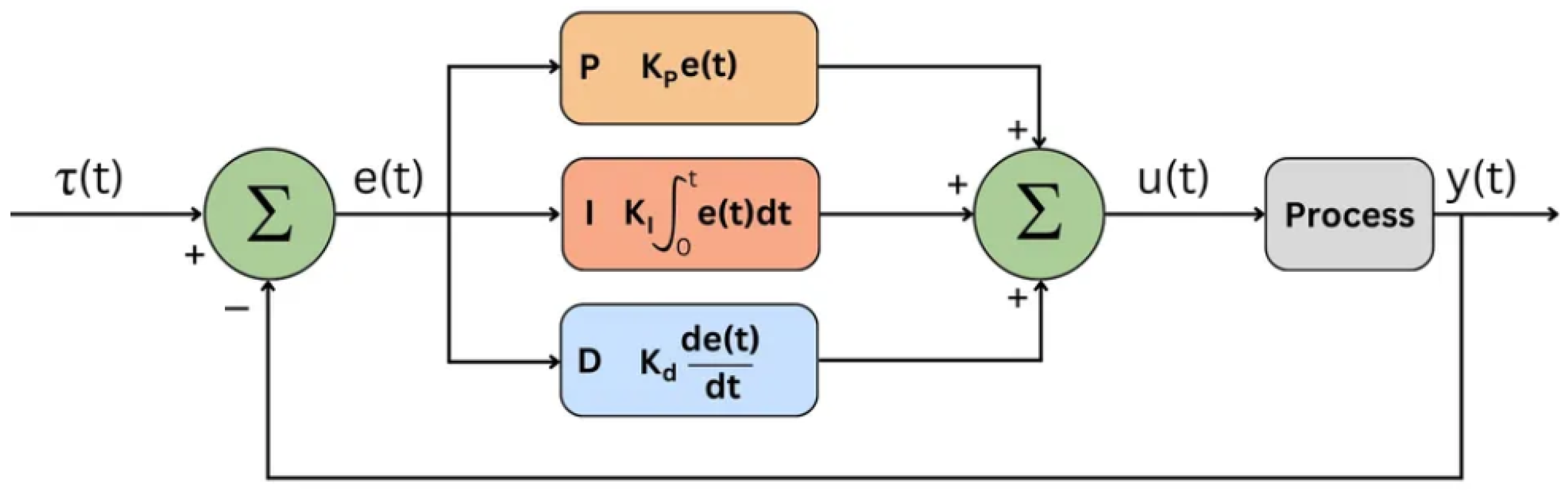
PID control (Figure 7) offers a pragmatic alternative for cost-sensitive applications with limited computational resources, operating in trajectory error without requiring detailed dynamic modeling [37]. The control law is expressed as:

$$u\left(t\right)=K_{P}e\left(t\right)+K_I{\int }_0^{t}e\left(\tau \right)d\tau +K_D{\displaystyle \frac{de\left(t\right)}{dt}}$$

(10)

where $e\left(t\right)$ represents the tracking error and $K_P$, $K_I$, and $K_D$ are the proportional, integral, and derivative gains, respectively.

This approach is effective for pick-and-place operations, material handling, and collaborative robotics with moderate accuracy requirements, such as the Pick&Eat device (Figure 10a). The controller can be implemented in either joint space for direct motor control or task space for end-effector positioning, depending on specific application demands.

Linear Quadratic Regulator (LQR) provides optimal control for linear systems that require resource optimization, such as autonomous mobile robotics and energy-constrained systems [37]. This approach minimizes a quadratic cost function that explicitly balances tracking accuracy against control effort:

$$J={\int }_0^{\infty }\left(x^{T}Qx+u^{T}Ru\right)dt$$

(11)

where x represents the state vector, u denotes the control input, and Q, R are positive definite weighting matrices that establish the trade-off between tracking performance and energy consumption. The resulting optimal control law is as follows:

$$u=-Kx$$

(12)

where K is determined by solving the associated Riccati equation, which provides guaranteed stability and optimal performance for the specified cost criterion. LQR proves to be valuable in battery-powered systems, aerial robotics, and energy-constrained applications, such as the saffron harvesting device (Figure 14b) and the HeritageBot (Figure 14c).

The selection of the control strategy depends on the dynamics of the robot, the requirements of the task, and the availability of the model. Computed torque control suits submillimeter precision applications, PID control addresses cost-sensitive systems with moderate accuracy needs, and LQR optimizes energy-efficient operations in resource-constrained environments.

5.2. Mid-Level Control

Mid-level control generates and tracks operational space trajectories, translating them into joint-level commands compatible with the robot’s kinematics, effectively bridging high-level planning and physical execution.

A central aspect of mid-level control is the use of the differential kinematics relationship, previously introduced in Section 3, which describes the mapping between joint velocities and the end-effector velocity in Cartesian space. To implement trajectory tracking in the operational space, it is often necessary to solve the inverse problem, i.e., to determine $\dot{q}$ given a desired end-effector velocity ${\dot{x}}_d$. This is typically addressed using the Moore–Penrose pseudoinverse of the Jacobian, yielding:

$${\dot{q}}_d=J^{†}\left(q\right){\dot{x}}_d+\left(I-J^{†}J\right)z$$

(13)

where $J\left(q\right)$ is the Jacobian matrix, $J^{†}\left(q\right)$ is the pseudoinverse of the Jacobian, and z is a free vector that belongs to the null space of the Jacobian. This vector allows for the optimization of secondary objectives such as energy minimization, redundancy resolution, or collision avoidance. This approach is particularly relevant in redundant robots, where the number of degrees of freedom exceeds the dimensionality of the task space.

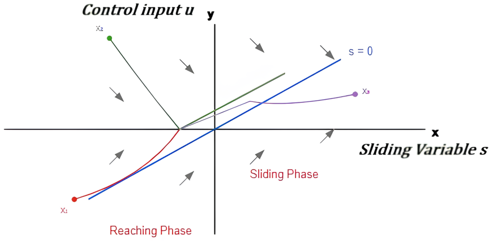
Regarding robustness in the presence of dynamic uncertainties or external disturbances, a widely adopted strategy is Sliding Mode Control (SMC) (Figure 8), known for its ability to ensure reliable performance even under significant parameter variations [38].

The principle behind SMC is the definition of a sliding surface:

$$s=\dot{e}+\lambda e$$

(14)

where e is the tracking error between the desired trajectory and the actual trajectory and $\lambda$ is a positive scalar parameter that defines the dynamics of the error. The control law takes the form:

$$u=-K\left(x\right)-\rho \left(x\right)\mathrm{sgn}\left(s\right)$$

(15)

where $K\left(x\right)$ represents the continuous component of the control and $\rho \left(x\right)$ is a gain term that ensures robustness against uncertainties and disturbances. The discontinuous term $\mathrm{sgn}\left(s\right)$ drives the trajectory of the system toward the sliding surface, along which the system dynamics are governed solely by the surface properties, making the behavior insensitive to variations in unmodeled parameters.

However, SMC typically requires smoothing techniques to mitigate chattering effects from control signal discontinuities. In general, Mid-level control coordinates robot motion with precision and robustness, translating specifications into executable strategies suited to physical system constraints.

5.3. High-Level Control (Supervisory Control)

High-level control integrates advanced computational tools for continuous diagnosis, intelligent adaptation, and real-time optimization, ensuring proper system functioning and adaptive responsiveness under uncertain or dynamic conditions.

A fundamental element of this level is the adoption of the digital twin, a dynamic virtual model of the physical system that enables continuous and accurate monitoring. The digital twin is implemented using advanced estimation techniques, including the Extended Kalman Filter (EKF), which optimally fuses sensor measurements with predictions from the robot’s nonlinear mathematical model [37]. The updated state estimate is given by:

$${\widehat{x}}_{k+1}=f({\widehat{x}}_k,u_k)+K_k\left(y_k-h\left({\widehat{x}}_k\right)\right)$$

(16)

where ${\widehat{x}}_k$ is the state estimate at time k, $u_k$ is the control input, $y_k$ is the observed measurement, $f(·)$ and $h(·)$ represent the state evolution model and the observation function, respectively, and $K_k$ is the Kalman gain that balances the weighting of the innovation error, providing the best estimate under noise and uncertainties.

To ensure compliance with safety constraints, such as those of the ISO 10218 standard [39], the control architecture incorporates critical limits (speed, work area, exclusion zones, emergencies) directly into the supervision system. A real-time monitoring module, based on sensors and a digital twin, constantly checks compliance with these constraints. In the event of a violation, the system triggers safe stops or adjusts control parameters, integrating safety into the automatic decision-making process and ensuring proactive, standards-compliant risk management.

In dynamic and uncertain environments, high-level control also employs adaptive control strategies that allow real-time modification of controller parameters to maintain optimal performance. This adaptation is typically formulated as a system of differential equations for parameter estimation $\widehat{\theta }$:

$$\dot{\widehat{\theta }}=-\mathsf{\Gamma }ye$$

(17)

where $\mathsf{\Gamma }$ is a positive adaptive gain defined by the user, y is the system output, and e represents the tracking or estimation error. This law ensures that the controller updates its parameters based on the observed error, allowing a more flexible and resilient response to changing operating conditions or degradation phenomena.

To further enhance predictive performance and operational constraint management, high-level control often implements Model Predictive Control (MPC), Figure 9 [40].

MPC solves, in real time, an optimization problem over a finite horizon N, minimizing a cost function that balances tracking accuracy and control input variation:

$$u_k=arg\underset{(u_k,\dots ,u_{k+N-1})}{min}\sum _{i=0}^{N-1}{∥x_{k+i+1}-x_{k+i+1}^d∥}_Q^2+{∥u_{k+i}-u_{k+i}^{ref}∥}_R^2$$

(18)

subject to the discrete dynamic model:

$$x_{k+1}=A_k{x}_k+B_k{u}_k$$

(19)

where $x_k$ represents the control signal calculated at time instant k, $x_{k+i+1}^d$ and $u_{k+i}^{ref}$ are the reference trajectories for the state and the input, respectively, and Q and R are positive definite weighting matrices that define the relative importance of the monitoring objectives and energy consumption or the control effort. The system matrices $A_k$ and $B_k$ are continuously updated in real time through the digital twin, accounting for dynamic changes such as structural modifications or varying environmental conditions.

Real-time adaptation enables MPC to maintain high performance in complex scenarios. The architecture utilizes high-performance computational resources (multicore processors, GPUs, embedded platforms) to ensure sufficient bandwidth for online optimization and continuous digital twin synchronization.

In summary, high-level control provides an integrated framework that utilizes virtual models, estimation techniques, and predictive optimization to supervise and improve the behavior of the robotic system, ensuring robustness and efficiency.

6. Robotic System Prototyping

Physical prototyping represents the essential link between digital models and real systems, enabling the experimental verification of design solutions. This phase validates functional, kinematic, and structural specifications while detecting differences between simulated and real behavior. Physical prototypes enable verification of ergonomics, accessibility, and maintainability aspects that virtual environments cannot accurately assess. This reduces design risks by identifying critical issues before production. The systemic approach ensures consistency between digital models and physical prototypes, reducing the number of validation iterations. Material selection is guided by Product Design Specifications (PDS), considering key factors such as mechanical loads, geometric accuracy, weight, environmental conditions, and processing requirements.

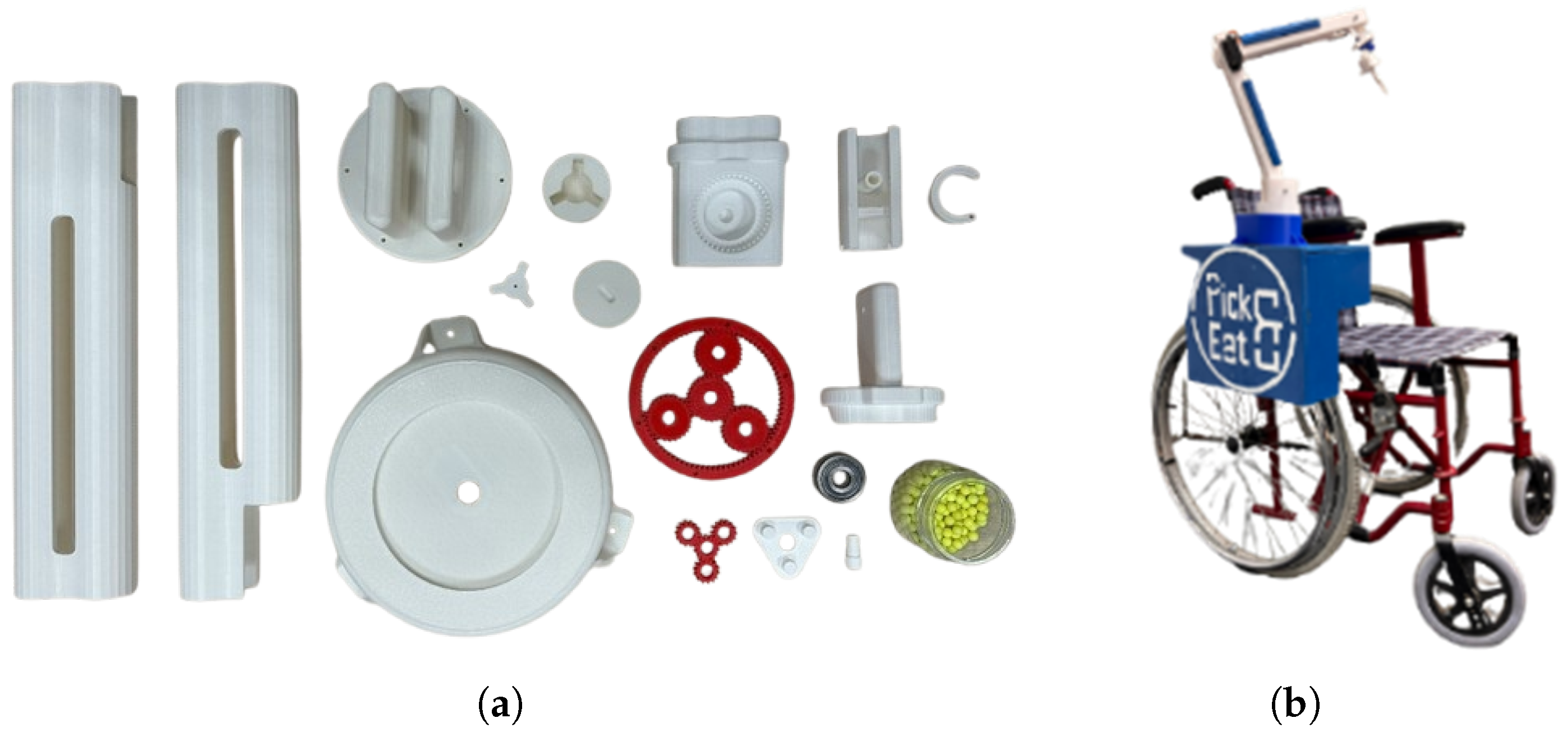
For low-load components or those intended for preliminary functional tests, 3D printed materials (PLA, PETG) are preferred due to their low cost, production speed, and ability to generate complex geometries with rapid iterations (Figure 10).

Figure 10. Robotic device prototyping phases: (a) 3D printed components; (b) complete prototype of the Pick&Eat (University of Calabria, Rende, Italy) robot ready for functional testing [41].

Figure 10. Robotic device prototyping phases: (a) 3D printed components; (b) complete prototype of the Pick&Eat (University of Calabria, Rende, Italy) robot ready for functional testing [41].

Structural elements subjected to high stress require machined metals (aluminum, steel, light alloys) with traditional technologies (milling, turning, cutting) for superior dimensional accuracy and reliability. Advanced materials (reinforced nylon, polycarbonate, and composites) meet specific functional requirements, such as flexibility, transparency, or thermal and chemical resistance. Established prototyping strategies include Commercial Off-The-Shelf (COTS) components, such as actuators, sensors, or pre-assembled frames, and hybrid solutions that combine different materials and technologies, accelerating development while optimizing performance.

An effective prototype must accurately reproduce the characteristics of the CAD model, including tolerances, dimensions, and kinematics, while replicating the intended functionality, consolidating design choices for subsequent industrialization phases.

7. Experimental Validation

This section presents the experimental validation of the proposed framework, applied to a 4-DOF robotic manipulator designed to assist in feeding [41]. Validation is the crucial link between the preliminary analyses described in Section 3.1, Section 4, and Section 5 and the prototype development. This phase verifies the accuracy of the model, the effectiveness of the control strategy, and the system performance under realistic operating conditions.

7.1. Kinematic Validation and Workspace Verification

The initial validation concerns the geometric performance of the system, verified through an experimental mapping of the work area obtained with a high-precision optical tracking system. The data collected allow us to confirm the kinematic models obtained with the Denavit–Hartenberg convention (Equation (1)) and the formulations of the forward and inverse kinematics equations (Equations (2) and (4)). Figure 1a shows the prototype schematic according to the DH parameters, while Figure 4b presents the kinematic and dynamic analysis used for motion planning. The experimental results highlight a good match between the theoretical predictions and the real measurements.

The accuracy and repeatability of the end-effector positioning are tested in different regions of the workspace by comparing experimental measurements with theoretical tolerances. These tests directly validate the inverse kinematic solutions and the differential kinematic relationships defined in the mathematical framework presented in Section 3.1, providing a quantitative assessment of the model fidelity.

7.2. Validation of Dynamic Performance and Energy Balance

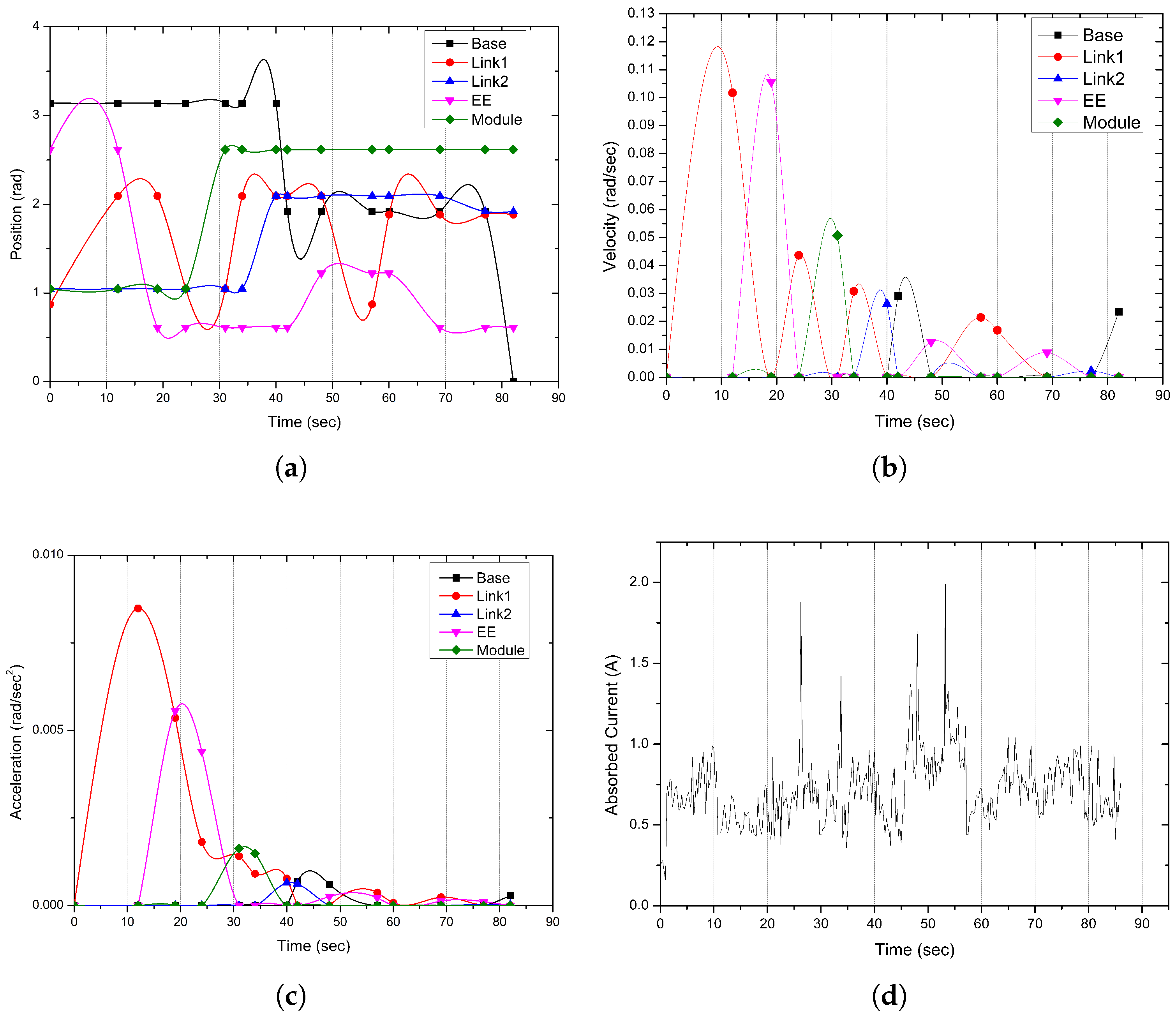
The validation extends to the temporal and dynamic performances by executing planned trajectories and simultaneously measuring position, velocity, acceleration, and torque at the actuator level. The collected experimental data are analyzed by comparing them with the solutions of Equation (8). Specifically, the time evolution of the position, shown in Figure 11a, the velocity in Figure 11b, and the acceleration in Figure 11c, are each evaluated against the predicted dynamic behavior. Furthermore, the electrical current absorbed by the servomotors, presented in Figure 11d, is used to assess the consistency between the energetic demand and the model-based torque requirements.

Figure 5b highlights the crucial role of motor sizing and torque requirement assessment, which are directly related to motion dynamics. Accurately assessing this step ensures that the actuator can deliver the required torque along the entire planned trajectory.

At the same time, energy balance verification confirms the consistency between mechanical and electrical energy within acceptable tolerances, as shown in Figure 11d. Parametric sensitivity analysis identifies the key parameters that influence the dynamic response, supporting calibration and validating the procedures described in Section 3.2.

7.3. Structural Integrity and Mechanical Behavior Assessment

Structural behavior is analyzed under static and dynamic loading conditions using strain gauges at critical points, allowing for comparison between experimental deformations and predictions obtained through finite element analysis. Specifically, Figure 5a illustrates the topological analysis of the structural configuration, while Figure 5b shows the evaluation of deformations and displacements under operational loading conditions.

These activities are part of the methodological context described in Section 4, where the integration between numerical simulations and experimental data guides the structural optimization process of the robotic system. Furthermore, impulsive perturbation tests allow one to evaluate the mechanical resistance and the response to vibrations, while accelerated fatigue tests, combined with non-destructive inspection techniques, support the analysis of the long-term structural reliability.

7.4. Validation of the Control System

The most advanced level of validation concerns the control system performance, verified through systematic tests in response to representative input signals. Evaluation metrics include settling time, overshoot, and steady-state error, confirming the effectiveness of the control architectures described in Section 5.

In addition, fault injection tests were performed to evaluate the system’s robustness against common faults, such as sensor malfunctions (e.g., loss of position feedback), actuator failures (e.g., partial or complete joint blockage), and communication interruptions between control modules. The system integrates real-time fault detection and isolation algorithms that continuously monitor signals. Upon detecting a fault, the system activates recovery mechanisms such as switching to redundant sensors, fallback modes, controlled shutdown, or reconfiguring control parameters, thus ensuring operational safety. These measures allow the manipulator to handle unexpected failures while maintaining functionality or stopping safely, confirming the system’s reliability under realistic conditions.

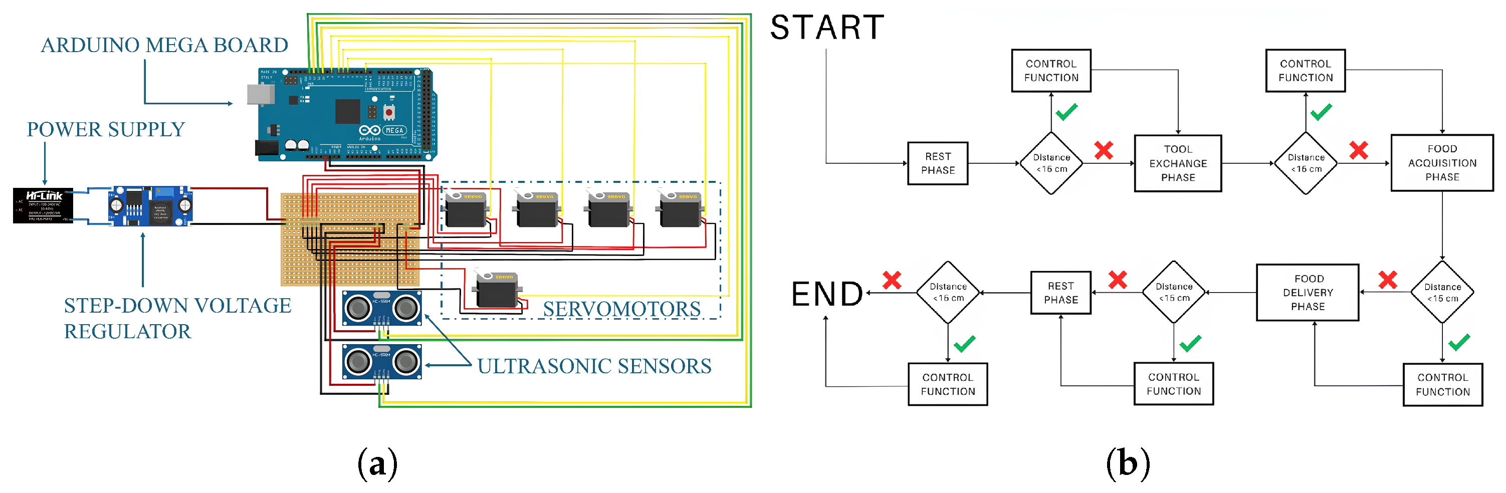
Safety constraints compliant with ISO 10218 [39], for industrial robots, and ISO/TS 15066 [42], for collaborative robots, are integrated across all control levels, from torque/speed limitation (Low-Level Control) to emergency stop protocols (High-Level Control).

Figure 12 shows the electrical connection diagram and the flow diagram of the control loop, illustrating the integration between safety logic and functional control. In this context, real-time monitoring algorithms continuously compare operating parameters with predefined safety limits, triggering progressive responses ranging from movement modification to complete system shutdown when necessary.

7.5. Final Validation in Real Operating Conditions

To complete the validation process, tests in real operating conditions were performed to evaluate the integrated behavior of the robotic system, verifying the coherence between the model, control, and physical response during representative task execution.

The photographic sequence of the task execution, shown in Figure 13, documents the system’s operational phases, offering a qualitative view of the precision and repeatability of the movement. The frontal and lateral images highlight the adherence of the actual behavior to the planned trajectories and compliance with safety constraints.

For collaborative robots like the device presented, human-in-the-loop evaluations were carried out during the validation phase to assess ergonomic comfort, reachability, and ease of use. Safety constraints derived from ISO/TS 15066 [42] were already incorporated during the CAD and simulation stages, ensuring that human–robot interaction zones complied with standardized collaborative workspace limits. This approach guaranteed that the final prototype respected both functional requirements and human-centered design principles.

The results obtained confirm the correct functioning of the system under all the previously analyzed profiles: kinematic, dynamic, structural, and control. The interaction between the different components (modeling, simulation, control, and experimental validation) has demonstrated a high reliability and a solid robustness of the device during the execution of realistic tasks.

8. Application Examples of the Proposed Methodology

The systematic design procedure described is highly adaptable in diverse fields, including rehabilitation, care, education, aerial robotics, manipulation, and agriculture, clearly demonstrating its broad and transversal applicability.

This methodology has enabled the development of diverse systems: upper limb rehabilitation devices (ReHArm shown in Figure 14a [43]), agricultural end-effectors (Figure 14b [44]), heritage monitoring platforms (HeritageBot shown in Figure 14c [45]), mobility assistance robots (RAISE shown in Figure 14d [46]), therapy devices (PaRRex shown in Figure 14e [47]), and surgical robots (Figure 14f [48]).

The robotic systems analyzed use a mix of modular hardware and adaptive software to meet specific needs in different areas. The ReHArm system (Figure 14a), for example, allows personalized upper limb rehabilitation thanks to adaptive stiffness control. For saffron harvesting, the semiautomatic device (Figure 14b) uses simulations and tests to reduce damage and contain costs. HeritageBot (Figure 14c), on the other hand, combines land and air movement in a modular platform suitable for cultural sites. The RAISE robot (Figure 14d) improves walking with adaptive actuation strategies, while PaRRex (Figure 14e) offers personalized upper limb therapy through real-time feedback. Finally, the needle insertion robot (Figure 14f) ensures precision in minimally invasive procedures, integrating advanced kinematics and imaging.

Table 2. Systematic methodology application analysis.

System	DoF	Primary Challenge	Methodology Focus	Validation Metric
Pick&Eat [41]	6	Autonomous feeding	Step 4 (Co-validation)	Precision accuracy
ReHArm [43]	5	Human–robot interaction	Step 2 (PDS uncertainty)	Safety compliance
Saffron Harvester [44]	4	Delicate manipulation	Step 3 (Multiobjective)	Damage minimization
HeritageBot [45]	8	Terrain navigation	Step 6 (Validation)	Environmental testing
RAISE [46]	6	Gait rehabilitation	Step 2 (Resilience)	Clinical outcomes
PaRRex [47]	7	Therapy protocols	Step 5 (Uncertainty)	Adaptive control
Surgical Robot [48]	8	Precision surgery	Step 6 (Statistical)	Accuracy validation
Finger Device [49]	3	Wearable integration	Step 5 (Optimization)	Ergonomic fit
Cable Robot [50]	4	Large workspace	Step 4 (Mathematical)	Tension distribution

shows the adoption in each system’s methodology, with PDS and modeling phases being central in all cases. Development cycles of 3–6 iterations reflect varying complexity and maturity requirements. The case studies demonstrate the flexibility and effectiveness of the methodology in creating robotic adaptable high-performance solutions in different applications, from rehabilitation to cultural heritage protection.

Figure 14. Illustrative examples of diverse robotic systems designed using the proposed systematic procedure, highlighting kinematics, dynamics, optimization, prototyping, and validation phases: (a) ReHArm system; (b) Saffron harvesting device; (c) HeritageBot; (d) lower limb rehabilitation robot RAISE; (e) Upper limb rehabilitation robot PaRRex; (f) surgical robot.

Figure 14. Illustrative examples of diverse robotic systems designed using the proposed systematic procedure, highlighting kinematics, dynamics, optimization, prototyping, and validation phases: (a) ReHArm system; (b) Saffron harvesting device; (c) HeritageBot; (d) lower limb rehabilitation robot RAISE; (e) Upper limb rehabilitation robot PaRRex; (f) surgical robot.

9. Conclusions

This work presents a structured framework for the development of an integrated robotic system that covers the entire lifecycle from concept to validation. The approach adopted combines analytical and computational tools, using consolidated mathematical formalisms (such as Denavit–Hartenberg parameters for kinematic modeling and Lagrangian dynamics), along with a hierarchical control architecture structured across multiple functional levels. This is supported by parametric optimization techniques and the use of CAD/CAE tools, with the aim of effectively connecting theoretical models with practical implementation. The framework’s key contribution is unifying traditionally disjointed methodologies within an iterative, validated process that minimizes the gap between theoretical modeling and practical application. Challenges remain in unstructured environments and multirobot system scalability.

Although the methodology has been validated on representative case studies, several challenges remain, particularly in managing interactions with unstructured environments and ensuring scalability in multirobot systems. While the approach demonstrates broad applicability to conventional robotic systems, specific limitations arise in the context of soft robotics and continuum manipulators. The mathematical foundations of the framework are based on rigid-body assumptions, which prove inadequate for systems characterized by infinite degrees of freedom and continuous deformation. Such systems require alternative modeling approaches, including continuum mechanics and specialized control paradigms.

Future research will focus on extending the proposed framework to accommodate emerging robotic paradigms and to enhance performance in unstructured and dynamic environments. Central to this effort is the systematic integration of advanced machine learning techniques capable of addressing modeling uncertainties and enabling real-time adaptation. In particular, reinforcement learning will be employed to support autonomous parameter tuning and behavioral adjustments without requiring detailed prior knowledge of the environment. Physics-Informed Neural Networks (PINNs) offer a promising avenue for bridging analytical models with data-driven learning, preserving the theoretical consistency of the framework while improving robustness in complex scenarios. To support autonomous operation in unstructured workspaces, the integration of computer vision and advanced perception systems will enable dynamic environment mapping and reliable obstacle avoidance, overcoming the limitations of conventional sensing strategies. Additionally, scalability in multirobot systems will be addressed through federated learning approaches, facilitating decentralized knowledge sharing and coordination across heterogeneous platforms.

Overall, these developments are aimed at enhancing the framework’s adaptability, autonomy, and generalizability while maintaining the methodological rigor and fundamental principles on which its current formulation is based. The primary goal is to evolve the framework in a direction that strengthens its reliability and consistency, while allowing for greater flexibility in adapting to diverse and complex application contexts. Special attention will be paid to standardizing the methodology, with the aim of making it a shared reference point in both industry and academic research. This standardization represents a crucial step towards creating a common language between research and production, facilitating effective technology transfer and the operational integration of innovative solutions in real-world scenarios. Therefore, the adoption of this framework has the potential to significantly streamline development processes, increase the reliability of robotic systems, and reduce the gap between the research and implementation phases. Ultimately, this will contribute to the realization of more robust, intelligent and efficient robotic solutions, capable of successfully addressing the challenges posed by advanced and dynamic real-world applications.

References

- Siciliano, B.; Sciavicco, L.; Villani, L.; Oriolo, G. Robotics: Modelling, Planning and Control; Springer: London, UK, 2009. [Google Scholar]
- Spong, M.W.; Hutchinson, S.; Vidyasagar, M. Robot Modeling and Control, 2nd ed.; John Wiley & Sons: Hoboken, NJ, USA, 2020. [Google Scholar]
- Kumar, V.; Michael, N. Opportunities and challenges with autonomous micro aerial vehicles. Int. J. Robot. Res. 2012, 31, 1279–1291. [Google Scholar] [CrossRef]
- Murray, R.M.; Li, Z.; Sastry, S.S. A Mathematical Introduction to Robotic Manipulation; CRC Press: Boca Raton, FL, USA, 2017. [Google Scholar]
- Billard, A.; Kragic, D. Trends and Challenges in Robot Manipulation. Science 2019, 364, eaat8414. [Google Scholar] [CrossRef] [PubMed]
- Zhao, Y.; Li, X.; Wang, Z.; Chen, M.; Liu, H. Resilience-based design methodology for tunnel construction robotics under uncertain geological conditions. Tunn. Undergr. Space Technol. 2025, 156, 106739. [Google Scholar]
- Brunton, S.L.; Proctor, J.L.; Kutz, J.N. Discovering Governing Equations from Data by Sparse Identification of Nonlinear Dynamical Systems. Proc. Natl. Acad. Sci. USA 2016, 113, 3932–3937. [Google Scholar] [CrossRef] [PubMed]
- Kober, J.; Bagnell, J.A.; Peters, J. Reinforcement Learning in Robotics: A Survey. Int. J. Robot. Res. 2013, 32, 1238–1274. [Google Scholar] [CrossRef]
- Mueller, A. An Overview of Formulae for the Higher-Order Kinematics of Lower-Pair Chains with Applications in Robotics and Mechanism Theory. Mech. Mach. Theory 2019, 142, 103594. [Google Scholar] [CrossRef]
- Craig, J.J. Introduction to Robotics: Mechanics and Control, 3rd ed.; Pearson Education India: Tamil Nadu, India, 2009. [Google Scholar]
- Duka, A.V. Neural Network Based Inverse Kinematics Solution for Trajectory Tracking of a Robotic Arm. Procedia Technol. 2014, 12, 20–27. [Google Scholar] [CrossRef]
- Ayyıldız, M.; Cetinkaya, K. Comparison of Four Different Heuristic Optimization Algorithms for the Inverse Kinematics Solution of a Real 4-DOF Serial Robot Manipulator. Neural Comput. Appl. 2016, 27, 825–836. [Google Scholar] [CrossRef]
- Featherstone, R. Exploiting Sparsity in Operational-Space Dynamics. Int. J. Robot. Res. 2010, 29, 1353–1368. [Google Scholar] [CrossRef]
- Khalil, W.; Dombre, E. Modeling, Identification and Control of Robots; Butterworth-Heinemann: London, UK, 2004. [Google Scholar]
- Azar, A.T.; Zhu, Q.; Khamis, A.; Zhao, D. Control Design Approaches for Parallel Robot Manipulators: A Review. Int. J. Model. Identif. Control 2017, 28, 199–211. [Google Scholar] [CrossRef]
- Lopez, B.T.; Slotine, J.-J.E. Universal Adaptive Control of Nonlinear Systems. IEEE Control Syst. Lett. 2021, 6, 1826–1830. [Google Scholar] [CrossRef]
- Corke, P.; Robotics, V. Control: Fundamental Algorithms in MATLAB; Springer Tracts in Advanced Robotics; Springer: Berlin/Heidelberg, Germany, 2011. [Google Scholar]
- Quigley, M.; Conley, K.; Gerkey, B.; Faust, J.; Foote, T.; Leibs, J.; Bergery, E.; Wheeler, R.; Ng, A.Y. ROS: An Open-Source Robot Operating System. ICRA Workshop Open Source Softw. 2009, 3, 5. [Google Scholar]
- Sung, C.; MacCurdy, R.; Coros, S.; Yim, M. Computational Robot Design and Customization. Robotica 2023, 41, 1–2. [Google Scholar] [CrossRef]
- Rus, D.; Tolley, M.T. Design, Fabrication and Control of Soft Robots. Nature 2015, 521, 467–475. [Google Scholar] [CrossRef] [PubMed]
- Nguyen-Tuong, D.; Peters, J. Model Learning for Robot Control: A Survey. Cogn. Process. 2011, 12, 319–340. [Google Scholar] [CrossRef] [PubMed]
- Wang, C.; Cheng, B. Design of a Robotic Gripper for Casting Sorting Robots with Rigid–Flexible Coupling Structures. Robotica 2024, 42, 2658–2676. [Google Scholar] [CrossRef]
- Emet, H.; Gür, B.; Dede, M.İ.C. The Design and Kinematic Representation of a Soft Robot in a Simulation Environment. Robotica 2024, 42, 139–152. [Google Scholar] [CrossRef]
- Gasparetto, A.; Takeda, Y.; Rosati, G. Editorial of the Special Issue: Innovative Robot Design for Special Applications. Robotica 2024, 42, 1712–1714. [Google Scholar] [CrossRef]
- Ulrich, K.T.; Eppinger, S.D. Product Design and Development; McGraw-Hill: New York, NY, USA, 2016. [Google Scholar]
- Cross, N. Engineering Design Methods: Strategies for Product Design; John Wiley & Sons: Hoboken, NJ, USA, 2021. [Google Scholar]
- Dieter, G.E.; Schmidt, L.C. Engineering Design, 6th ed.; McGraw-Hill Education: New York, NY, USA, 2021. [Google Scholar]
- Shabana, A.A. Dynamics of Multibody Systems; Cambridge University Press: Cambridge, UK, 2020. [Google Scholar]
- Boothroyd, G.; Dewhurst, P.; Knight, W.A. Product Design for Manufacture and Assembly; CRC Press: Boca Raton, FL, USA, 2010. [Google Scholar]
- Tao, F.; Qi, Q.; Wang, L.; Nee, A.Y.C. Digital twins and cyber–physical systems toward smart manufacturing and industry 4.0: Correlation and comparison. Engineering 2019, 5, 653–661. [Google Scholar] [CrossRef]
- Sahu, V.S.D.M.; Samal, P.; Panigrahi, C.K. Modelling, and Control Techniques of Robotic Manipulators: A Review. Mater. Today Proc. 2022, 56, 2758–2766. [Google Scholar] [CrossRef]
- Reckhaus, M.; Hochgeschwender, N.; Paulus, J.; Shakhimardanov, A.; Kraetzschmar, G.K. An Overview about Simulation and Emulation in Robotics. In Proceedings of the SIMPAR, Darmstadt, Germany, 15–16 November 2010; pp. 365–374. [Google Scholar]
- Zhang, L.; Wang, Q.; Chen, M. Optimized Trajectory Tracking for Robot Manipulators with Uncertain Dynamics: A Composite Position Predictive Control Approach. Electronics 2023, 12, 4548. [Google Scholar] [CrossRef]
- Wang, X.; Liu, Y.; Zhang, H. Neural Network Adaptive Hierarchical Sliding Mode Control for the Trajectory Tracking of a Tendon-Driven Manipulator. Chin. J. Mech. Eng. 2024, 37, 172. [Google Scholar]
- Rodriguez, A.; Silva, P.; Martinez, J. Unity and ROS as a Digital and Communication Layer for Digital Twin Application: Case Study of Robotic Arm in a Smart Manufacturing Cell. Sensors 2024, 24, 5680. [Google Scholar] [CrossRef] [PubMed]
- Liu, B.; Rocco, P.; Zanchettin, A.M.; Zhao, F.; Jiang, G.; Mei, X. A Real-Time Hierarchical Control Method for Safe Human–Robot Coexistence. Robot.-Comput.-Integr. Manuf. 2024, 86, 102666. [Google Scholar] [CrossRef]
- Kang, Z.; Li, H.; Wang, Y.; Yu, H. A Review of Hierarchical Control Strategies for Lower-Limb Exoskeletons in Children with Cerebral Palsy. Machines 2025, 13, 442. [Google Scholar] [CrossRef]
- Islam, S.; Liu, X.P. Robust Sliding Mode Control for Robot Manipulators. IEEE Trans. Ind. Electron. 2010, 58, 2444–2453. [Google Scholar] [CrossRef]
- ISO 10218-1; Robotics—Safety Requirements. Part 1: Industrial Robots. International Organization for Standardization, ISO: Geneva, Switzerland, 2025.
- Rawlings, J.B.; Mayne, D.Q.; Diehl, M. Model Predictive Control: Theory, Computation, and Design, 2nd ed.; Nob Hill Publishing: Madison, WI, USA, 2017. [Google Scholar]
- Leone, S.; Giunta, L.; Rino, V.; Mellace, S.; Sozzi, A.; Lago, F.; Curcio, E.M.; Pisla, D.; Carbone, G. Design of a Wheelchair-Mounted Robotic Arm for Feeding Assistance of Upper-Limb Impaired Patients. Robotics 2024, 13, 38. [Google Scholar] [CrossRef]
- ISO/TS 15066; Robots and Robotic Devices—Collaborative Robots. ISO: Geneva, Switzerland, 2016.
- Leone, S.; Laribi, M.A.; Castillo-Castañeda, E.; Carbone, G. An Interactive Combined Mechatronic Approach to Enhance Upper Limb Rehabilitation. In Advances in Italian Mechanism Science; Springer Nature: Cham, Switzerland, 2024; pp. 19–26. ISBN 978-3-031-64569-3. [Google Scholar]
- Denarda, A.R.; Bertetto, A.M.; Carbone, G. Designing a Low-Cost Mechatronic Device for Semi-Automatic Saffron Harvesting. Machines 2021, 9, 94. [Google Scholar] [CrossRef]
- Ceccarelli, M.; Cafolla, D.; Russo, M.; Carbone, G. HeritageBot Platform for Service in Cultural Heritage Frames. Int. J. Adv. Robot. Syst. 2018, 15, 1729881418790692. [Google Scholar] [CrossRef]
- Major, Z.Z.; Vaida, C.; Major, K.A.; Tucan, P.; Brusturean, E.; Gherman, B.; Birlescu, I.; Craciunaș, R.; Ulinici, I.; Simori, G.; et al. Comparative Assessment of Robotic versus Classical Physical Therapy Using Muscle Strength and Ranges of Motion Testing in Neurological Diseases. J. Pers. Med. 2021, 11, 953. [Google Scholar] [CrossRef] [PubMed]
- Vaida, C.; Birlescu, I.; Pisla, A.; Carbone, G.; Plitea, N.; Ulinici, I.; Gherman, B.; Puskas, F.; Tucan, P.; Pisla, D. RAISE—An Innovative Parallel Robotic System for Lower Limb Rehabilitation. In New Trends in Medical and Service Robotics; Carbone, G., Ceccarelli, M., Pisla, D., Eds.; Mechanisms and Machine Science; Springer: Cham, Switzerland, 2018; pp. 293–302. [Google Scholar]
- Pisla, D.; Vaida, C.; Birlescu, I.; Hajjar, N.A.; Gherman, B.; Radu, C.; Plitea, N. Risk Management for the Reliability of Robotic Assisted Treatment of Non-resectable Liver Tumors. Appl. Sci. 2020, 10, 52. [Google Scholar] [CrossRef]
- Carbone, G.; Ceccarelli, M.; Capalbo, C.E.; Caroleo, G.; Morales-Cruz, C. Numerical and Experimental Performance Estimation for a ExoFing—2 DOFs Finger Exoskeleton. Robotica 2022, 40, 1820–1832. [Google Scholar] [CrossRef]
- Khadem, M.; Inel, F.; Carbone, G.; Slimane Tich Tich, A. A Novel Pyramidal Cable-Driven Robot for Exercising and Rehabilitation of Writing Tasks. Robotica 2023, 41, 3463–3484. [Google Scholar] [CrossRef]