Abstract
In response to the safety control requirements of heavy robot operations, to address the problems of cumbersome, time-consuming, poor accuracy and low real-time performance in robot end contact force estimation without force sensors by using traditional manual modeling and identification methods, this paper proposes a new contact force estimation method for heavy robots without force sensors by combining CNN-GRU and force transformation. Firstly, the CNN-GRU machine learning method is utilized to construct the robot Joint Motor Current-Joint External Force Model; then, the Joint External Force-End Contact Force Model is constructed through the Kalman filter and Jacobian force transformation method, and the robot end contact force is estimated by finally uniting them. This method can achieve robot end contact force estimation without a force sensor, avoiding the cumbersome manual modeling and identification process. Compared with traditional manual modeling and identification methods, experiments show that the proposed method in this paper can approximately double the estimation accuracy of the contact force of heavy robots and reduce the time consumption by approximately half, with advantages such as convenience, efficiency, strong real-time performance, and high accuracy.
1. Introduction
Nowadays, robots are being increasingly applied across various industries, with growing attention to the safety of both work objects and personnel during robot operations [1,2,3]. The ability of robots to perceive environmental contact forces during operation is crucial to ensuring safe execution. Generally, the force control of the operation process is realized based on the feedback of force sensors. However, adding additional large range force sensors to the heavy robot undoubtedly increases the complexity and cost of the system, and there are also some problems such as substantial size, drift, and hysteresis. Therefore, ways to make the robot accurately estimate the contact force and perform force control operation without force sensors have gradually become a hot research issue.
For robot contact force estimation methods without force sensors, many scholars have carried out relevant research, including the traditional contact force estimation based on analytical modeling and the contact force estimation based on machine learning. Sol et al. [4] and Hasanzadeh et al. [5] estimated the end-effector external force of the robot based on the identified robot dynamic model using the motor torque and motor angle. Stolt et al. [6] used joint micro-oscillationas torque feedforward compensation to then estimate the end-effector external force based on the joint motor current. Mitsantisuk et al. [7] estimated the end-effector grasping force through the motor torque and angle by using the Kalman filter method. Polverini et al. [8] proposed a sensorless observer which is optimized against the specified admittance and constraints. However, this method had a limitation in dealing with geometric uncertainties. Zhang et al. [9] and Sariylildiz et al. [10], proposed a joint torque estimation method based on motor angle, joint angle, and motor current, respectively, using a dual-encoder joint structure model or a dual-mass resonance model to achieve robot joint torque estimation. Han et al. [11] proposed a novel interaction force estimation scheme capable of estimating the interaction forces for industrial robots with high precision in the absence of force sensors. Firstly, the dynamic model of a class of industrial robots is established by model identification methods. Furthermore, a high-order finite-time observer (HOFTO) was established to estimate the interaction forces.
From the discussion above, it is evident that traditional contact force estimation methods rely on accurate modeling and complex parameter identification. However, robots are inherently complex MIMO (Multiple-Input Multiple-Output) nonlinear systems characterized by time-varying, strongly coupled, and highly nonlinear dynamic behaviors. Compared to medium- and light-load robots, heavy-duty robots are typically equipped with high-torque motors, RV reducers, and reinforced structural components to support large payloads. As a result, they exhibit increased weight and inertia, more pronounced structural deformations, slower motion, and significant nonlinear friction within the transmission system. These factors further complicate force estimation, making it challenging for conventional analytical modeling approaches to ensure both accuracy and robustness in heavy-duty robotic applications. In particular, the challenge of obtaining a comprehensive and precise analytical expression for the robotic mechanical model becomes even more pronounced in heavy-duty robots. Greater inertia, structural deformations, and actuator nonlinearities further amplify the complexity of force estimation. The accuracy of force estimation depends heavily on the validity of the modeling approach and the appropriateness of the data processing methods. Consequently, traditional model-based force estimation techniques often suffer from reduced precision and robustness when applied to heavy-duty robots.
Since it is extremely difficult to establish a mechanical model that accurately estimating the end contact force by using only the limited motion state information of the robot body in practice, some scholars have turned to machine learning methods to build robot mechanical models without force sensors. Aksman et al. [12] used robot dynamics and motor current feedback to estimate the joint torque of robots, adopting an adaptive neural network to learn the unknown parameters of the robot dynamics model. Jin et al. [13] proposed a parametric robot dynamics model based on rigid-body dynamics (RBD), combined with a non-parametric compensator trained with multilayer perception (MLP) to eliminate errors resulting from the former modeling. Exploiting such a two-layer modeling, a high-accuracy robot dynamics description is obtained, achieving better model accuracy than either the RBD model or the MLP model itself. Model uncertainties are compensated by adopting a radial basis neural networks approach. Ngo et al. [14] proposed an adaptive wavelet neural network control law, using a wavelet neural network (WNN) to estimate the interaction force/torque of multi-moving manipulators. Martin et al. [15] used the joint torque to identify the transient contact force in the actual working process of the robot, and the RNN model was adopted. Stanko Kružić et al. [16] used the base force sensor and the neural network method to estimate the magnitude of the force at the robot end and obtain the estimated error on the triaxial force. Liu et al. [17] proposed a sensorless scheme to estimate the unknown contact force induced by the physical interaction with robots. The model-based identification scheme is initially used to obtain the dynamic parameters. Then, neural learning of friction approximation is designed to enhance the estimation performance for robotic systems subject to model uncertainty. Zhang et al. [18] proposed a force estimation algorithm calibration method and a fuzzy PD control assembly method based on convolutional neural network (CNN) supervised learning to solve the problem of the insufficient estimation accuracy of the interference observer. Zhao, Y et al. [19] proposed a new reinforcement learning neural network (RLNN) algorithm framework that can realize the force perception of multi-contact robots and has the advantages of input variable dimension optimization and a lightweight network structure. Tseng et al. [20] proposed an adaptive hybrid position/force control method based on a fuzzy neural network (FNN). The uncertain parts of the dynamic model and system are estimated by the FNN.
In summary, most existing studies primarily focus on external force estimation for light-load robots (load capacity under 50 kg) without force sensors, as referenced in these papers [16,19,21], while research explicitly targeting contact force estimation for heavy-load robots (load capacity above 100 kg) remains relatively scarce. At the same time, there is also little research on the model parameter selection and real-time performance of force estimation using machine learning methods. However, our heavy-duty robot is primarily used for handling and assembling large loads. During operation, it is crucial to avoid excessive contact force between the load and the environment to prevent potential damage to the load. Therefore, accurately estimating the contact force is essential for ensuring operational safety. The method proposed in this paper is relatively general and can be applied to estimate the contact force between the robot’s end-effector and the environment in other robotic operations. In terms of time and cost, the method presented in this paper has clear advantages compared to using a force/torque sensor. If a force/torque sensor is used for contact force measurement on the existing robot, modifications to the robot’s mechanical, electrical, and software systems are necessary. This is followed by procurement, production, assembly, debugging, and calibration. Each of these steps adds time costs (estimated to be at least one month) and economic costs (the procurement of a high-capacity multi-dimensional force sensor alone could cost tens of thousands of RMB). In contrast, the method presented in this paper eliminates the time and economic costs associated with these modifications, offering a more efficient and cost-effective solution.
The research object of this article is a heavy robot with a load capacity of more than 500 kg. We proposed a combined CNN-GRU and a force transformation method based on a Kalman filter to estimate the contact force of the heavy robot without additional force sensors (cost saving), while avoiding the tedious manual modeling and identification process (convenient and efficient), thus realizing a lower-cost, more convenient, efficient, real-time, and higher-accuracy contact force estimate method to meet the requirements of heavy robot safety control without force sensors.
2. Overall Design Idea
Traditional robot contact force estimation methods, including dynamic estimation methods, generalized momentum observer methods, and velocity observer methods, etc., all require the accurate parameter identification and modeling for robots. However, since most robots without force sensors can only obtain limited motion state information, such as joint displacement, motor current, and velocity, traditional contact force estimation methods require complex modeling and tedious parameter identification using limited information, which is particularly challenging for building a joint friction model for a robot drive system.
Therefore, the proposed contact force estimation method avoids the tedious process of manual modeling and parameter identification, which include the following two parts: the first is using the CNN-GRU machine learning method to construct a Joint Motor Current-Joint External Force Model, and the second is using a Kalman filter and Jacobian force transformation to construct a Joint External Force-End Contact Force Model. By combining the Motor Current-Joint External Force Model with the Joint External Force-End Contact Force Model, the final end contact force is estimated. The entire algorithm design principle is shown in Figure 1. In this framework, the main input variables include the joint displacement, motor current, and velocity. The selection of these input variables is based on their ability to provide dynamic state information of the robot and their relationship with interaction forces. These input variables are first fed into the CNN-GRU-based Joint Motor Current-Joint External Force Model to obtain the joint external force. Subsequently, the obtained joint external force is processed through the Kalman filter and Jacobian force transformation-based Joint External Force-End Contact Force Model to estimate the final end contact force.
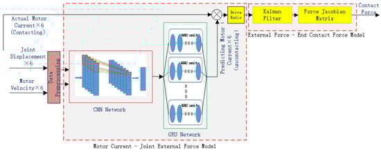
Figure 1.
Principle of the contact force estimation method.
One of the reasons why the CNN-GRU network is used to build a Motor Current-Joint External Force Model is that during robot motion, the multi-dimensional state data that the robot can directly perceive, such as joint displacement, motor current, and motor velocity, are spatially related to the robot contact force, and these state data also constitute time series data, meaning that the robot current motion state is closely related to a previous motion state in time. Since CNNs (Convolutional Neural Networks) are good at processing data with spatial structure features, and GRU (Gated Recurrent Unit) networks are good at processing time series data, this paper proposes a contact force prediction model that combines CNN and GRU. The prediction model has the advantages of both methods, and it can efficiently extract features from the motion data of the robot so as to construct a Motor Current-Joint External Force Model that is difficult to determine by traditional manual modeling and identification methods.
3. Motor Current-Joint External Force Model
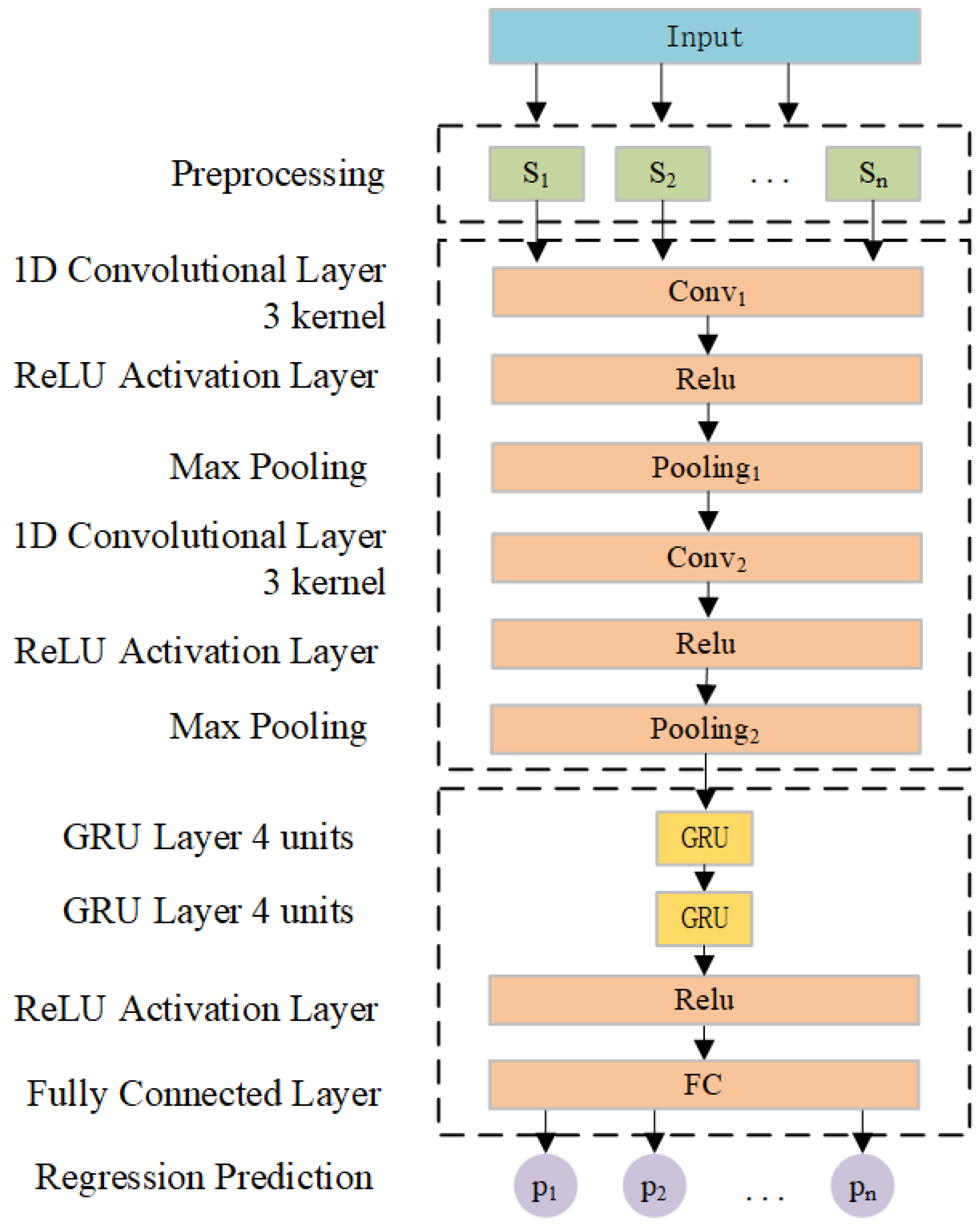
In this study, a CNN-GRU machine learning method is employed to construct a robot motor current-joint force model. The CNN is a deep neural network composed of convolutional layers, pooling layers, and fully connected layers alternately. It employs a local connection and weight-sharing method to reduce the number of weights in the entire network, facilitating network optimization and lowering model complexity. CNN is essentially a multi-layer perceptron that can efficiently extract multi-dimensional data features. The Gated Recurrent Unit (GRU) model further optimizes the gating structure of the traditional LSTM model. Using update and reset gates to extract essential input information and selecting the output information, the GRU solves the problems of gradient disappearance or explosion, and it can better capture long-term dependencies, performing well in time series prediction. Given that CNN models excel in extracting spatial data features and GRU models are particularly adept at modeling temporal data, we amalgamated these strengths to construct a unified CNN-GRU model. Initially, the CNN model is employed to extract features from the robot’s motion state information, followed by utilizing the GRU model to predict and regress the temporal feature information of robot motion. This approach facilitates the accurate prediction of the joint current of robots at non-contact states.
The structure of our constructed CNN-GRU model is depicted in Figure 2. The input data include the position of six joints and the motor velocity feedback from six drive units, etc. The prediction model includes one preprocessing layer, two convolutional layers, two max pooling layers, two CNN ReLU activation layers, two GRU layers, one ReLU activation layer, and one fully connected layer. The preprocessing layer processes input motion state data before feeding them into the convolutional layer. The latter consists of two one-dimensional convolutional layers. Both pooling layers employ maximum pooling with identical parameter settings. Subsequently, outputs from the convolutional layer are flattened and their dimensions adjusted prior to being passed to the GRU layer. Finally, the model generates the predicted joint current values of the robot at a non-contact state through the fully connected layer. In addition, the optimization objective of training the CNN-GRU network is to minimize the discrepancy between predicted values and true values through backpropagation. The mean square error (MSE) serves as the model loss function and can be defined as follows:
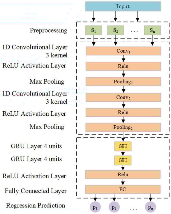
Figure 2.
CNN-GRU-based joint current prediction model.
In Equation (1), represents the root mean squared error. N is the total number of samples. denotes the observed (true) value for the i-th sample. represents the predicted value for the i-th sample.
Where represent the time step and prediction duration length. A smaller RMSE value indicates a more effective predictive model. Subsequently, the parameters of the GRU-CNN model are optimized using the Adam optimizer algorithm to minimize the RMSE. This algorithm integrates momentum and adaptive learning rate concepts, automatically adjusting learning rates to expedite convergence. The formula for the Adam algorithm is as follows:
In Equation (2), is the updated parameter at time step t. is the parameter from the previous time step. is the learning rate, which controls the step size in the optimization process. is the first moment estimate (typically the exponentially weighted moving average of the gradient). is the bias-corrected second moment estimate (typically the exponentially weighted moving average of the squared gradient). is a small constant added for numerical stability to prevent division by zero.
Here, denotes the learning rate with a default value of ; prevents division by zero with a default value of ; and represents the gradient mean obtained through the following:
In Equation (3), is the exponential decay rate for the first moment estimate, typically set to a value like 0.9. is the first moment estimate from the previous time step. is the gradient of the loss function with respect to the parameter at the current time step.
represents the gradient variance obtained through the following:
In Equation (4), is the second moment estimate at time step t, which keeps track of the exponentially weighted moving average of squared gradients. is the exponential decay rate for the second moment estimate, typically set to a value like 0.999. is the gradient squared of the loss function with respect to the parameter at the current time step.
In this formula, represent the exponential decay rate, and represents the gradient at time t. Here, controls weight allocation with a default value of 0.9, while governs previous gradient square influence with a default value of 0.999. As each joint actual current driven by the actuator in a contact state encompasses the current at a non-contact state and the current of the external force at a contact state, the current of the external force at a contact state is derived by subtracting the predicted non-contact state joint current with CNN-GRU from the actual contact state joint current. Finally, the external force for each joint is calculated by using the joint external force currents and transmission coefficients (motor torque coefficient, transmission ratio, etc.) as follows:
In Equation (5), is the real-time collected motor current at joint i, at time t, in the contact operation state. is the predicted motor current for joint i in the non-contact operation state, typically estimated using a model such as CNN-GRU. is the estimated additional motor current caused by external forces when the joint is in contact.
In Equation (6), is the estimated external torque at joint i during contact operation due to external forces. is the motor torque constant, which converts current into torque, typically measured in N·m/A. is the predicted current without external force, calculated based on joint angle and angular velocity , typically estimated using models such as CNN-GRU.
Before applying the CNN-GRU model, the model needs to be trained using data on the robot’s motion state. First, the robot is made to perform a wide range of repeated movements within the workspace in a non-contact state, and the joint displacement, motor speed, and current feedback from the six actuators during the movement are recorded. Then, the joint displacement and motor speed feedback from the six actuators are used as the model input, and the motor current feedback from the six joints are used as the model output to train the CNN-GRU model. When the CNN-GRU model is trained, it is then imported into the robot controller. After that, the robot performs contact operations, and the joint displacement, motor speed, and current feedback from the six actuators are collected in real time. Finally, the joint external force of the robot is calculated using Equations (5) and (6).
4. Joint External Force-End Contact Force Model
We constructed the Joint Motor Current-Joint External Force Model of the robot through the above machine learning method. It is observed that the actual motor current collected by the robot at a contact state includes the current of the joint at a non-contact state and (t), the current of the joint external force at a contact state. The CNN-GRU prediction of the current component has covered the uncertain and nonlinear relationship between the joint torque and the current of the robot at a non-contact state, but there still exists joint noise in the current component due to the contact operation of the robot, and then, the obtained external force of the robot joint also contains noise. Therefore, it is necessary to design a filter to estimate the joint external force obtained by the Motor Current-Joint External Force Model, followed by using the Jacobian matrix of the robot force for calculating the end contact force.
Estimation of Joint External Forces
Assuming independent Gaussian white noise as the observation noise for each joint torque, we need to filter each joint external force separately. In terms of filter selection, the Kalman filter-based observer demonstrates effective observation on random signals where process noise and measurement noise can be approximated as white noise. Compared with the Butterworth filter and other digital filters, the parameters of the Kalman filter are more convenient to adjust, with easier control over the smoothing effect of the estimated value without the problem of selecting an initial value. Hence, this paper employs the Kalman filter method for estimation with a specific design as follows:
State prediction equation:
Variance prediction equation:
Kalman gain equation:
State estimation equation:
State estimation variance equation:
Initial state estimation variance:
The definition of the terms in the above formulas is as follows: represents the estimated torque value after filtering for joint i; represents the torque value before filtering; represents the torque value state prediction; indicates the variance prediction value; stands for the Kalman gain; t represents the corresponding time; refers to the process noise variance; represents the measurement noise variance; and i denotes the sequence number for robot joints. Experiments indicate better filtering effect when initial values and .
For the selection of process noise variance , the low-speed commutation part of the robot joint can easily cause motor torque disturbance, which leads to the large process noise of the motor current. Therefore, the process noise variance is designed as a function related to the speed of the manipulator joint as follows:
where is the noise variance of the joint torque process corresponding to the joint velocity located in the normal working interval, is the noise variance of the joint torque process corresponding to the joint velocity located in the abnormal working interval (nearby 0 rpm). The larger the value of , the larger the adaptive joint velocity range. represents the order of the error change of the learned model between the adapted joint velocity range and the unadapted joint velocity range, and the more gradual the change of the model error caused by the two speed intervals, the smaller the value.
5. Experiment and Result Analysis
This section begins with an introduction to our experimental environment used for validating our proposed method, and then, the data set acquisition and preprocessing required for the experiment are carried out. After that, the model parameter selection experiment is conducted. When the model parameters are determined, the contact force estimation accuracy experiment and the contact force real-time experiment are performed, and the experimental results are analyzed.
5.1. Experimental Environment
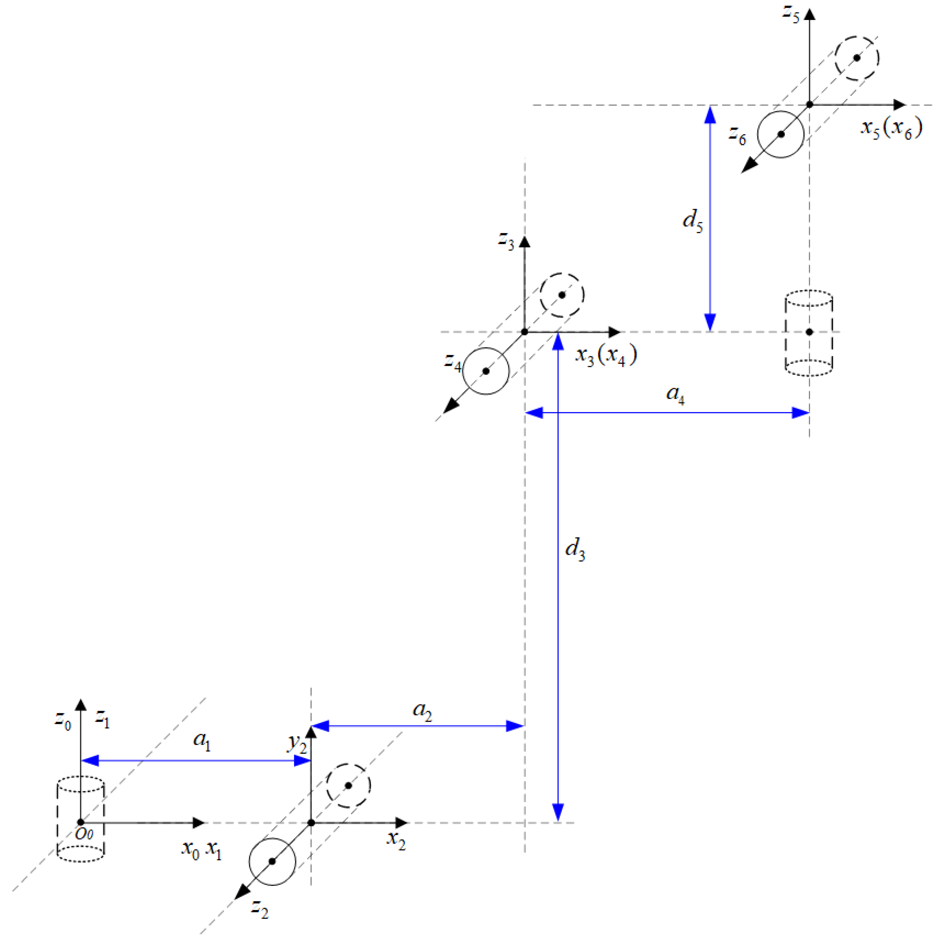
The 6-DOF robot configuration and the definition of the coordinate system used in this paper are shown in Figure 3. As shown in Figure 3, the robot joints 1, 2, 4, 5, and 6 are rotary joints, which are primarily composed of a servo motor and an RV reducer in the drive system. Joint 3 is a translational joint, mainly consisting of a servo motor, gearbox, and ball screw. The robot’s controller uses an industrial computer equipped with an Intel I7 motherboard and runs the VxWorks 6.9 real-time operating system. By combining the force estimation method proposed in this paper, impedance control can be applied to the robot’s end-effector, enabling the robot to exhibit a certain degree of compliance. The parameters of the improved D-H are shown in Table 1.
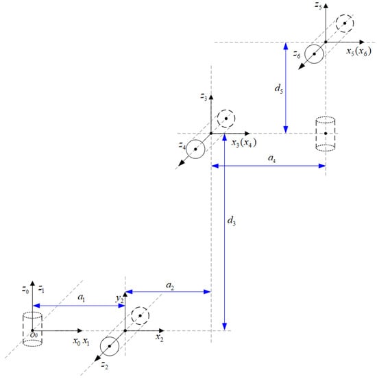
Figure 3.
Six-axis coordinate system of a robotic arm.

Table 1.
D-H parameters of the robotic arm.
The modified D-H parameters are shown in Table 1.
For developing a CNN-GRU model aimed at modeling the Motor Current-Joint External Force Model, the deep learning framework used in this paper is pytorch, which supports C++, python, and other languages. It can run on both CPU and GPU, and it has strong portability. Each experiment uses the exact same hardware computing platform, the experiment hardware configuration is Intel i7-13700H CPU, graphics card RTX 4060, and memory 16 GB. The software is configured with Ubuntu 16.04 64-bit operating system, Anaconda 3, Python 3.7, pytorch 2.0.1, and CUDA 10.0.
5.2. Dataset Acquisition and Preprocessing
Taking a specific operational trajectory of the robot as an example, the operation cycle of the trajectory is 20 s. The robot is programmed to execute 20 movements from the starting point to the end point in a non-contact state, following this operational trajectory. During each movement, robot motion state data, including six joint displacement, the motors’ speed, and current feedback from the six drivers, are recorded at a sampling frequency of 50 Hz. The selected trajectory in this study is based on the robot’s actual operating conditions, focusing on contact force estimation during its operation along the trajectory. Therefore, this trajectory does not represent the robot’s entire workspace. The dataset utilized in this study comprises time series data representing these motion states, totaling 20,000 sets of data, which providing a comprehensive set of operational trajectory motion states. An 80% portion of this dataset is allocated for training purposes, while the remaining 20% served as test data. Since the range of data corresponding to different motion state variables is different, in order to make each feature have the same measurement scale, all data need to be normalized before CNN-GRU neural network training to avoid poor training effect. The normalization method is as follows:
where, is the i element of the sampled data, is the normalized data element, is the maximum value of the sampling sequence of this element, and is the minimum value of the sampling sequence of this element. Through the above equation, we can map the whole sampling sequence data to the interval [−1,1].
5.3. Model Parameter Selection Experiment
The selection process for model parameters primarily focuses on evaluating how varying numbers of GRU layers and nodes, CNN convolution kernel sizes, different learning rates, and Dropout sizes influence model prediction accuracy using the root mean square error (RMSE) as an evaluation metric.
Firstly, in order to verify the influence of the number of GRU layers and nodes on the prediction accuracy of the model, we set the number of GRU layers to 1, 2, 3, and 4 and the nodes of each layer to 32, 64, 128, and 256, so as to construct the prediction model with different numbers of GRU layers and nodes. The experimental results are shown in Table 2.
Table 2.
Impact of different layer and node counts on model prediction accuracy.
It can be seen that when the number of layers of the GRU is 2, the accuracy of the model is higher on different numbers of nodes. With the increase in the number of nodes in the GRU, the accuracy can be increased to a certain extent, but when the number of nodes exceeds 64, it will be reduced to a certain extent, and then the region will be stable. Therefore, the number of GRU layers selected is two and the number of nodes is 64 in this paper.
Then, in order to verify the influence of the convolution kernel size of the CNN on the prediction accuracy of the model, we set the convolution kernel size of CNN to be 1 × 1, 1 × 2, 1 × 3, and 1 × 4, respectively, so as to construct feature recognition models with different convolution kernel sizes. At the same time, the GRU model uses the above optimal number of layers and nodes. The experimental results are shown in Table 3.
Table 3.
Impact of different convolutional kernel sizes on model accuracy.
It is evident that the CNN-GRU model achieves its highest accuracy when employing a 1 × 2 convolution kernel. Subsequent increases in the size of the convolution kernel lead to an escalation in model training parameters, accompanied by a decrease in accuracy. Consequently, this paper sets the size of the convolution kernel for the CNN layer at 1 × 2.
Furthermore, to investigate the impact of learning rate magnitude on prediction accuracy, four distinct learning rates are selected for evaluation. Generally, lower learning rates result in slower parameter updates and prolonged training time, while higher learning rates cause oscillations in loss function output and hinder convergence. The experimental results are shown in Table 4.
Table 4.
Impact of the learning rate on prediction accuracy.
The experimental results presented in Table 4 demonstrate that a learning rate of 0.001 yields high prediction accuracy; hence, this paper adopts a learning rate of 0.001 for model training.
Finally, to assess the influence of Dropout size on prediction accuracy, four different Dropout values are chosen for evaluation. The experimental results are shown in Table 5.
Table 5.
Impact of Dropout on prediction accuracy.
The experimental findings displayed in Table Figure 2 reveal that setting Dropout at 0.2 leads to high prediction accuracy; therefore, this paper adopts a Dropout value of 0.2.
In summary, after the experimental process of model parameter selection, the structure and parameters of the CNN-GRU model proposed in this paper are determined as shown in Table 6.
Table 6.
CNN-GRU model experimental parameters.
5.4. Experiment on Contact Force Estimation Error
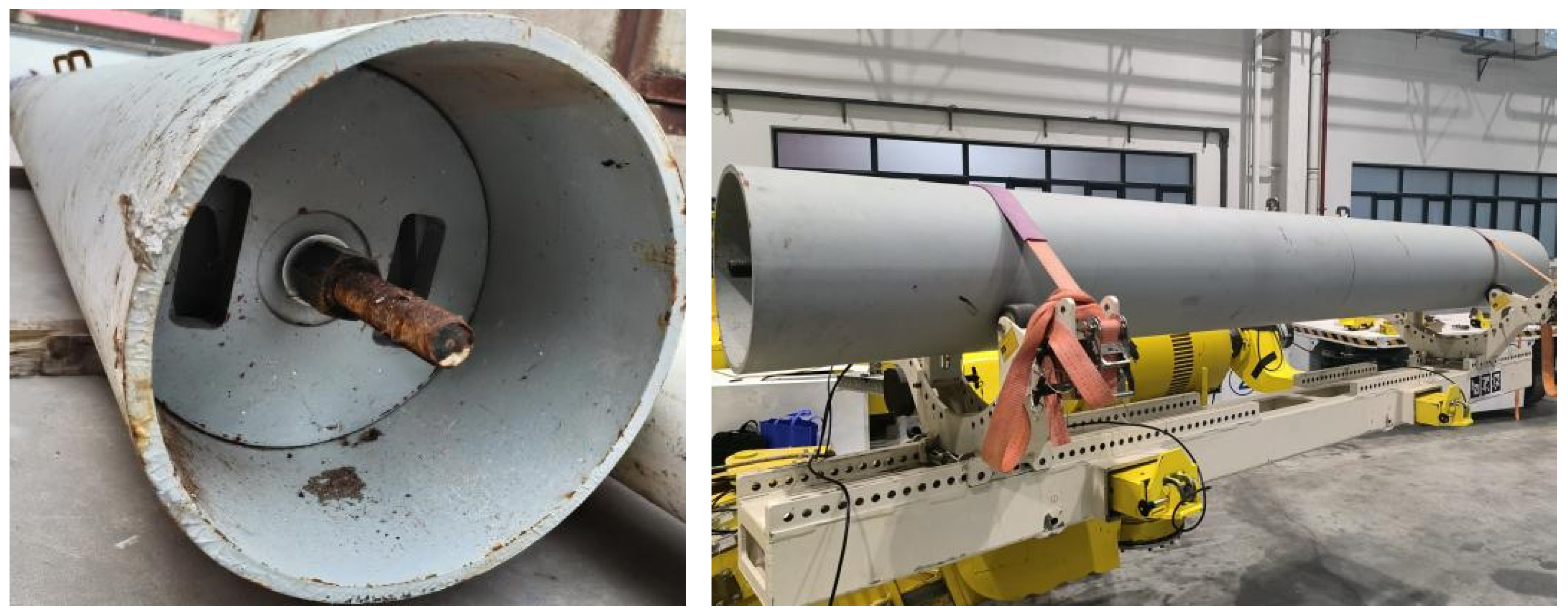
To evaluate whether our proposed contact force estimation method can accurately predict the contact force for robots without force sensors, while still taking a certain working trajectory of the robot as an example, we let the robot carry loads of 100 kg, 300 kg, and 500 kg in a non-contact state to build a robot joint current prediction model through the CNN-GRU machine learning method. The load is a steel cylinder with counterweights inside, 25 kg each, which is shown in Figure 4.

Figure 4.
Robot running with the load at the end of the manipulator.
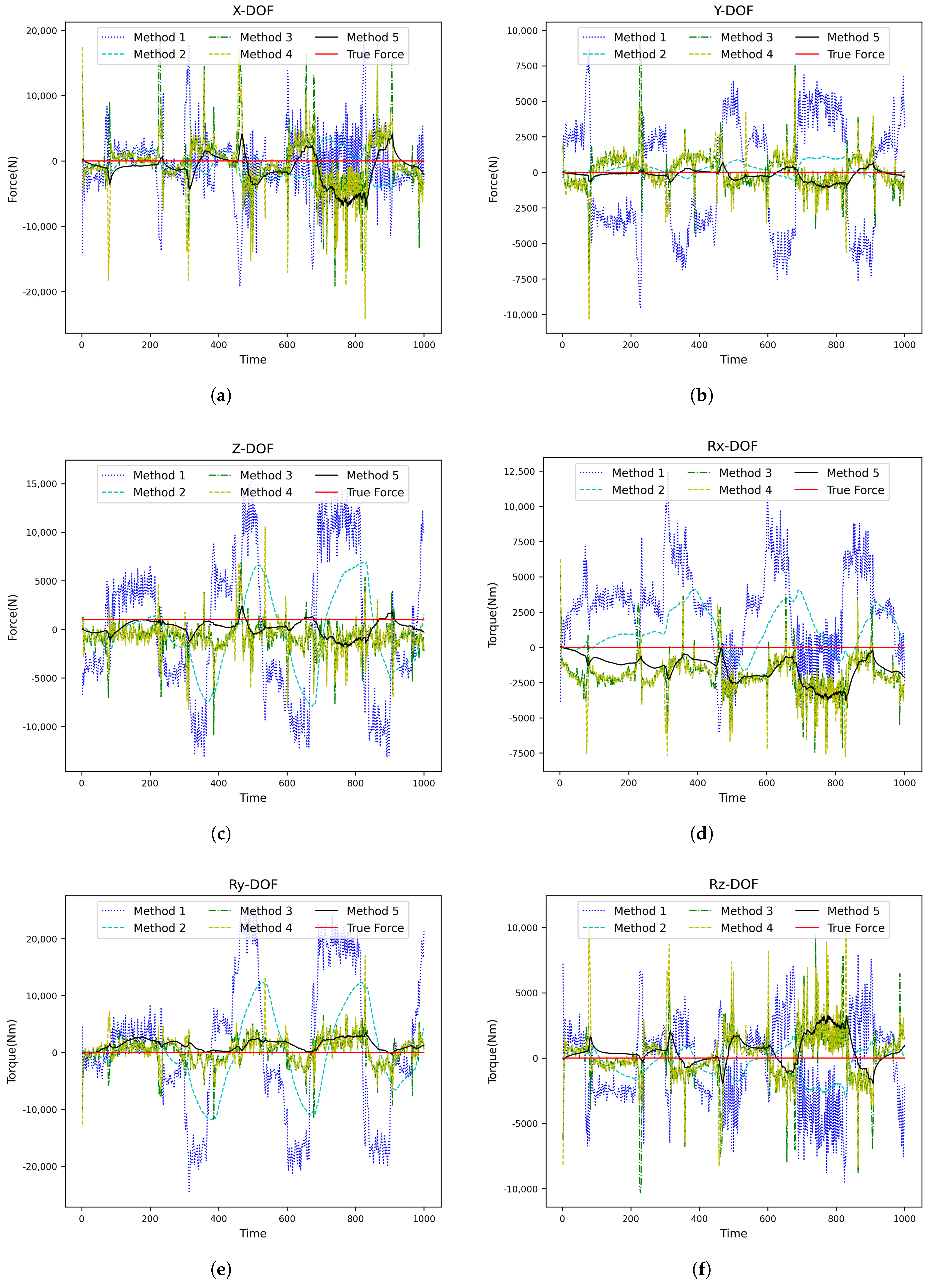
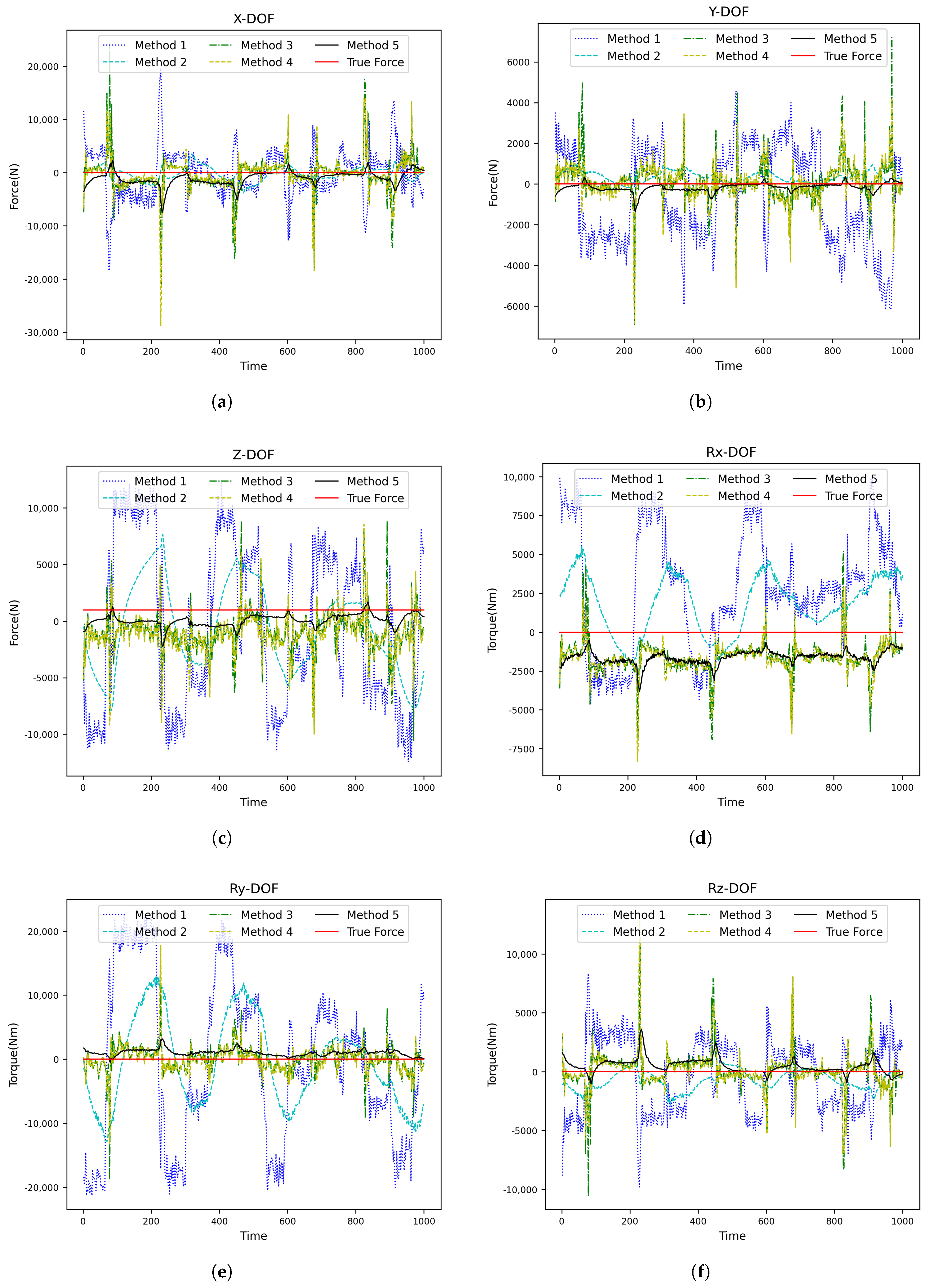
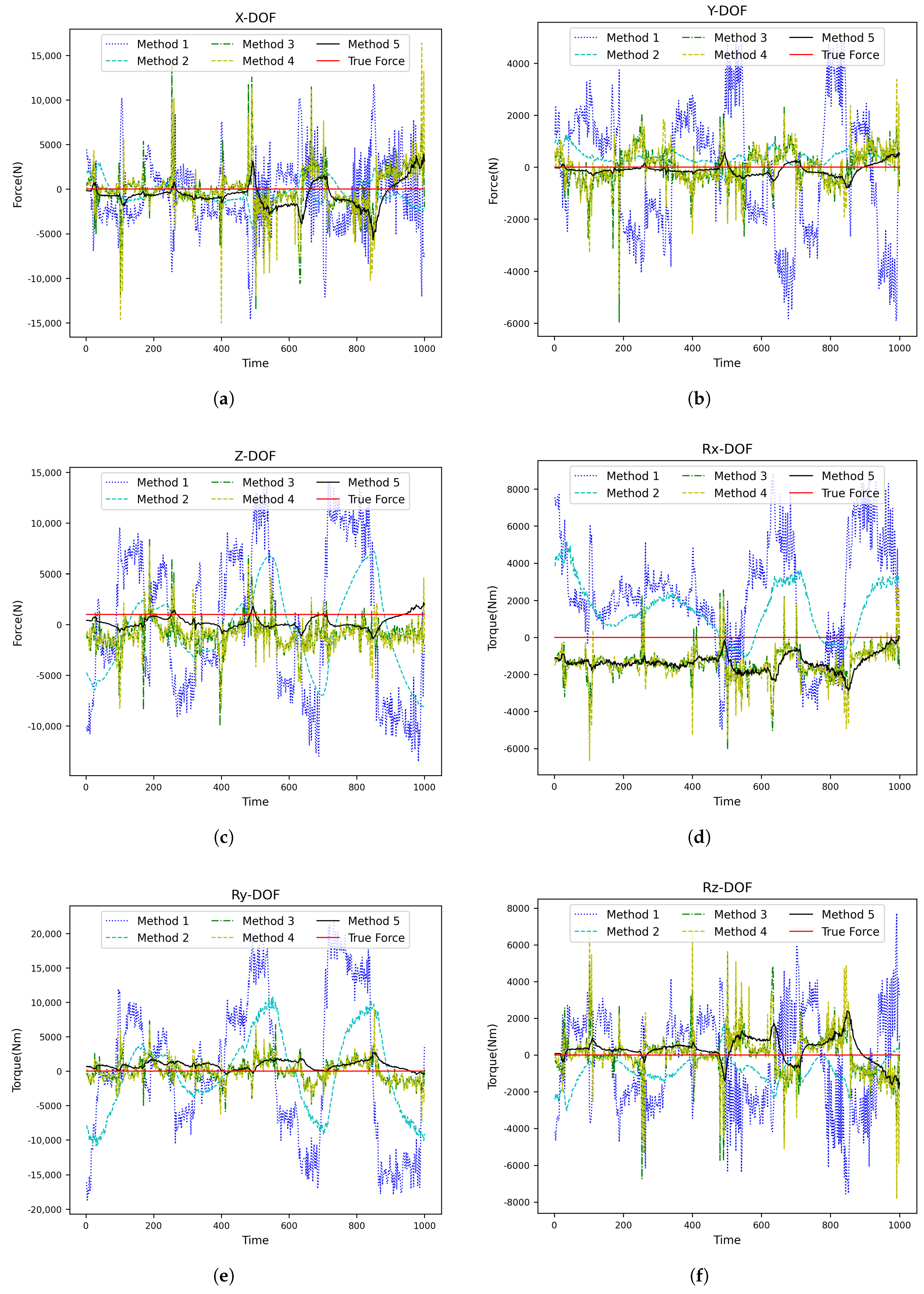
After that, an additional 100 kg is loaded onto the end of the robot to simulate the end contact force, and the robot movement is repeated five times from the starting point to the endpoint, according to the working trajectory under loads of 100 kg, 300 kg, and 500 kg. A total validation set comprising data from six joint displacements of the robot and motor speed/current feedback from six drivers during each movement was recorded (15,000 pieces). Finally, we utilize the RMSE as an evaluation index for comparative experiments across the five contact force estimation methods outlined in Table 7. The experimental results are shown in Figure 5, Figure 6 and Figure 7 and Table 8, Table 9, Table 10 and Table 11. In these figures, it can be observed that Method 5, represented by the black line, is the closest to the ground truth. This demonstrates that the proposed method is the most suitable choice for the scenario described in this paper.
Table 7.
Contact force estimation methods.
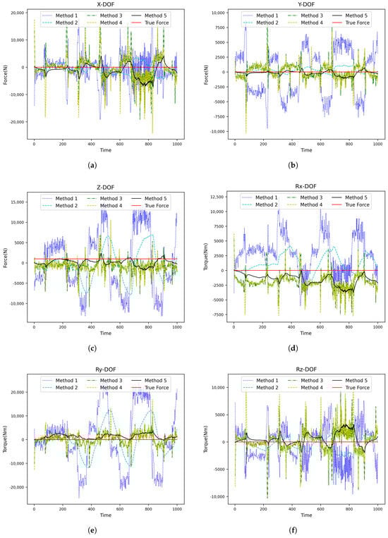
Figure 5.
Prediction results of each contact force estimation method when the robot load is 100 kg (one movement): (a) X-DOF, (b) YX-DOF, (c) Z-DOF, (d) Rx-DOF, (e) Ry-DOF, and (f) Rz-DOF.
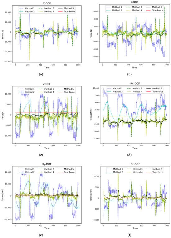
Figure 6.
Prediction results of each contact force estimation method when the robot load is 300 kg (one movement): (a) X-DOF, (b) YX-DOF, (c) Z-DOF, (d) Rx-DOF, (e) Ry-DOF, and (f) Rz-DOF.
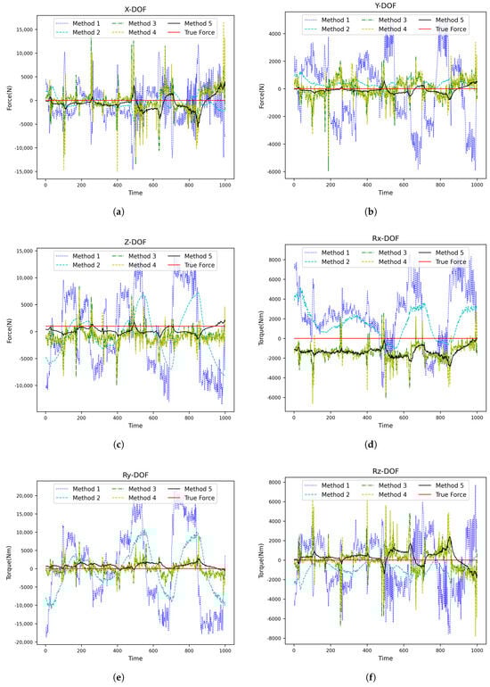
Figure 7.
Prediction results of each contact force estimation method when the robot load is 500 kg (one movement): (a) X-DOF, (b) YX-DOF, (c) Z-DOF, (d) Rx-DOF, (e) Ry-DOF, and (f) Rz-DOF.
Table 8.
Average error of different contact force estimation methods when the robot load is 100 kg.
Table 9.
Average error of different contact force estimation methods when the robot load is 300 kg.
Table 10.
Average error of different contact force estimation methods when the load is 500 kg.
Table 11.
Root mean square average of contact force errors in 6 degree of freedom directions under different loads.
According to our experimental results on robot contact force estimation error without force sensors from the above, the following can be derived: In the absence of a Kalman Filter, the error of contact force estimation using traditional manual modeling and parameter identification (Method 1) is much larger than that using machine learning (Method 3 and Method 4), and it is difficult to use in the actual operation of robot. After adding a Kalman smoothing filter into both the traditional manual modeling/parameter identification method and the CNN-GRU method, separately (Method 2 and Method 5), noticeable convergence was observed regarding the contact force estimation error. Method 5 has the smallest contact force estimation error, and its average contact force estimation error is about half of that of Method 2. At the same time, as the robot load increases, the contact force estimation error of Method 5 gradually decreases.As shown in the Table 11.Therefore, the combined approach utilizing CNN-GRU along with a Kalman filter proposed herein substantially enhances contact force estimation accuracy compared to traditional methods.
5.5. Real-Time Experiments on Contact Force Estimation
In order to evaluate whether the contact force estimation method proposed in this paper can predict more quickly, the operation time of the five contact force estimation methods shown in Table 7 is taken as the real-time evaluation index for comparison. The experimental data are based on the above 5000 validation set data, and the experimental results are shown in Table 12.
Table 12.
Comparison of time metrics across different methods.
From the real-time experimental results, the average time of estimating the contact force once by using the above five methods is less than 1.5 ms for all cases, which can meet the needs of real-time contact force estimation for the robot. Among them, the time of estimating the contact force once by using the traditional analytical modeling method (Method 1 and Method 2) is longer (>1 ms). However, the time of estimating the contact force once by using the machine learning method (Method 3, Method 4, and Method 5) is shorter (<0.5 ms), which is about half of the time consumption of the traditional contact force estimation method. Therefore, the proposed methods in this paper have obvious advantages in the real-time performance of contact force estimation.
6. Conclusions
This paper presents a new method for estimating contact force in robots without force sensors by integrating a CNN-GRU model and force transformation. A CNN-GRU neural network model is constructed to predict contact forces, effectively extracting robot motion data. The Motor Current-Joint External Force Model is trained, which is challenging to determine by using traditional manual modeling and identification methods. Additionally, the Joint External Force -End Contact Force Model is established by combining a Kalman smoothing filter and Jacobian force transformation method to estimate the robot end contact force. Compared with traditional manual modeling and identification methods, experiments show that the proposed method in this paper can approximately double the estimation accuracy of the contact force of heavy-duty robots and reduce the time consumption by approximately half. Thus, it lays a technical foundation for the safe operation of such robots.
While achieving accurate contact force estimation and force control without the use of force sensors remains a highly challenging task, it is undeniable that this direction holds significant potential for future development. Beyond the industrial heavy-duty robot applications discussed in this paper, the proposed method also shows great promise in broader fields such as medical robotics, service robotics, and agricultural robotics. In future work, we will conduct further research and exploration, focusing on developing more efficient machine learning methods tailored to kinematic and dynamic modeling, with the goal of extending robust and reliable sensorless contact force estimation techniques to a wider range of potential application scenarios.
Author Contributions
Conceptualization, P.W. and H.D.; methodology, P.W., H.D. and L.S.; software, P.L., L.S., W.D. and Y.B.; validation, P.W., H.D., W.D. and L.S.; formal analysis, P.W., W.D. and L.S.; investigation, P.W. and H.D.; resources, P.W. and H.D.; data curation, P.L., Y.B. and W.D.; writing—original draft preparation, P.W., H.D. and P.L.; writing—review and editing, W.D. and Y.B.; visualization, L.S.; project administration, P.W. and H.D.; funding acquisition, P.W. All authors have read and agreed to the published version of the manuscript.
Funding
This research was funded by the China State Shipbuilding Corporation (CSSC) Application Innovation Project, grant number 626011202. The APC was funded by the CSSC.
Institutional Review Board Statement
Not applicable.
Informed Consent Statement
Not applicable.
Data Availability Statement
Data are contained within the article.
Conflicts of Interest
Authors Peizhang Wu, Pengfei Li and Yifei Bao were employed by the company 713th Research Institute of China State Shipbuilding Corporation Limited. The remaining authors declare that the research was conducted in the absence of any commercial or financial relationships that could be construed as a potential conflict of interest.
References
- Papavasileiou, A.; Aivaliotis, S.; Mparis, P.; Mantas, P.; Makris, S. A Modular Framework of Robot Gripping Tools for Human Robot Collaborative Production Lines. Procedia CIRP 2024, 126, 164–169. [Google Scholar] [CrossRef]
- Zhou, X.; Wang, X.; Xie, Z.; Li, F.; Gu, X. Online Obstacle Avoidance Path Planning and Application for Arc Welding Robot. Robot. Comput. Integr. Manuf. Int. J. Manuf. Prod. Process. Dev. 2022, 78, 102413. [Google Scholar] [CrossRef]
- Khare, P.K.; Biswas, B.; Gupta, A. Collision Avoidance Using Potential Field in KUKA Robotic Arm. AIP Conf. Proc. 2024, 3122, 11. [Google Scholar] [CrossRef]
- Sol, E.D.; King, R.; Scott, R.; Ferre, M. External Force Estimation for Teleoperation Based on Proprioceptive Sensors. Int. J. Adv. Robot. Syst. 2014, 11, 52. [Google Scholar] [CrossRef]
- Hasanzadeh, S.; Janabi-Sharifi, F. Model-Based Force Estimation for Intra-Cardiac Catheters. IEEE/ASME Trans. Mechatron. 2016, 21, 154–162. [Google Scholar] [CrossRef]
- Stolt, A.; Robertsson, A.; Johannson, R. Robotic Force Estimation Using Dithering to Decrease the Low Velocity Friction Uncertainties. In Proceedings of the IEEE International Conference on Robotics and Automation, Seattle, WA, USA, 26–30 May 2015; pp. 3896–3902. [Google Scholar]
- Mitsantisuk, C.; Ohishi, K.; Katsura, S. Estimation of Action/Reaction Forces for Bilateral Control Using Kalman Filter. IEEE Trans. Ind. Electron. 2012, 59, 4383–4393. [Google Scholar] [CrossRef]
- Polverini, M.P.; Zanchettin, A.M.; Castello, S. Sensorless and Constraint-Based Peg-in-Hole Task Execution with a Dual-Arm Robot. In Proceedings of the IEEE International Conference on Robotics and Automation, Stockholm, Sweden, 16–21 May 2016; pp. 415–420. [Google Scholar]
- Zhang, H.W.; Ahmad, S.; Liu, G.J. Torque Estimation for Robotic Joint with Harmonic Drive Transmission Based on Position Measurements. IEEE Trans. Robot. 2015, 31, 322–330. [Google Scholar] [CrossRef]
- Sariyildiz, E.; Ohnishi, K. On the Explicit Robust Force Control via Disturbance Observer. IEEE Trans. Ind. Electron. 2015, 62, 1581–1589. [Google Scholar] [CrossRef]
- Han, L.; Mao, J.; Cao, P.; Gan, Y.; Li, S. Toward Sensorless Interaction Force Estimation for Industrial Robots Using High-Order Finite-Time Observers. IEEE Trans. Ind. Electron. 2022, 69, 7275–7284. [Google Scholar] [CrossRef]
- Aksman, L.M.; Carignan, C.R.; Akin, D.L. Force Estimation-Based Compliance Control of Harmonically Driven Manipulators. In Proceedings of the IEEE International Conference on Robotics and Automation, Roma, Italy, 10–14 April 2007; pp. 4208–4213. [Google Scholar]
- Jin, H.; Xiong, R. Contact Force Estimation for Robot Manipulator Using Semiparametric Model and Disturbance Kalman Filter. IEEE Trans. Ind. Electron. 2017, 65, 3365–3375. [Google Scholar]
- Ngo, V.T.; Liu, Y.C. Object Transportation Using Networked Mobile Manipulators Without Force/Torque Sensors. In Proceedings of the IEEE CACS, Taoyuan, Taiwan, 4–7 November 2018. [Google Scholar] [CrossRef]
- Karlsson, M.; Robertsson, A.; Johansson, R. Detection and Control of Contact Force Transients in Robotic Manipulation Without a Force Sensor. In Proceedings of the IEEE International Conference on Robotics and Automation, Brisbane, Australia, 21–25 May 2018; pp. 4091–4096. [Google Scholar]
- Kružić, S.; Musić, J.; Kamnik, R.; Papić, V. Estimating Robot Manipulator End-Effector Forces Using Deep Learning. In Proceedings of the 43rd International Convention on Information, Communication and Electronic Technology, Opatija, Croatia, 28 September–2 October 2020; pp. 1163–1168. [Google Scholar]
- Liu, S.; Wang, L.; Wang, V. Sensorless Force Estimation for Industrial Robots Using Disturbance Observer and Neural Learning of Friction Approximation. Robot. Comput.-Integr. Manuf. 2021, 71, 102168. [Google Scholar] [CrossRef]
- Zhang, T.; Liang, X.; Zou, Y. Robot Peg-in-Hole Assembly Based on Contact Force Estimation Compensated by Convolutional Neural Network. Control Eng. Pract. 2022, 120, 105012. [Google Scholar] [CrossRef]
- Zhao, Y.; Zheng, Q. RLNN: A Force Perception Algorithm Using Reinforcement Learning. Multimed. Tools Appl. 2024, 83, 60103–60115. [Google Scholar] [CrossRef]
- Tseng, B.R.; Jiang, J.Y.; Lee, C.H. Adaptive Position/Force Controller Design Using Fuzzy Neural Network and Stiffness Estimation for Robot Manipulator. Int. J. Fuzzy Syst. 2024. [Google Scholar] [CrossRef]
- Lao, Z.; Han, Y.; Chirikjian, G.S. How Heavy Is It? Humanoid Robot Estimating Physical Properties of Unknown Objects Without Force/Torque Sensors. arXiv 2021, arXiv:2104.09858. [Google Scholar]

Disclaimer/Publisher’s Note: The statements, opinions and data contained in all publications are solely those of the individual author(s) and contributor(s) and not of MDPI and/or the editor(s). MDPI and/or the editor(s) disclaim responsibility for any injury to people or property resulting from any ideas, methods, instructions or products referred to in the content. |
© 2025 by the authors. Licensee MDPI, Basel, Switzerland. This article is an open access article distributed under the terms and conditions of the Creative Commons Attribution (CC BY) license (https://creativecommons.org/licenses/by/4.0/).