Comparative Analysis of Energy Consumption and Performance Metrics in Fuel Cell, Battery, and Hybrid Electric Vehicles Under Varying Wind and Road Conditions

Abstract

As global initiatives to reduce greenhouse gas emissions and combat climate change expand, electric vehicles (EVs) powered by fuel cells and lithium-ion batteries are gaining global recognition as solutions for sustainable transportation due to their high energy conversion efficiency. Considering the driving range limitations of battery electric vehicles (BEVs) and the low efficiency of internal combustion engines (ICEs), fuel cell hybrid vehicles offer a compelling alternative for long-distance, low-emission driving with less refuelling time. To facilitate their wider scale adoption, it is essential to understand their energy performance through models that consider external weather effects, driving styles, road gradients, and their simultaneous interaction. This paper presents a microlevel, multicriteria assessment framework to investigate the performance of BEVs, fuel cell electric vehicles (FCEVs), and hybrid electric vehicles (HEVs), with a focus on energy consumption, drive systems, and emissions. Simulation models were developed using MATLAB 2021a Simulink environment, thus enabling the integration of standardized driving cycles with real-world wind and terrain variations. The results are presented for various trip scenarios, employing quantitative and qualitative analysis methods to identify the most efficient vehicle configuration, also validated through the simulation of three commercial EVs. Predictive modelling approaches are utilized to estimate a vehicle’s performance under unexplored conditions. Results indicate that trip conditions have a significant impact on the performance of all three vehicles, with HEVs emerging as the most efficient and balanced option, followed by FCEVs, making them strong candidates compared with BEVs for broader adoption in the transition toward sustainable transportation.

1. Introduction

The transportation sector plays a crucial role in global mobility and economic growth; however, it is among the most energy-intensive industries and a major contributor to greenhouse gas emissions [1,2]. In 2022, 74% of global CO₂ was released, and approximately 8 billion metric tons of CO₂ emissions were emitted only in 2023, making road vehicle transport the second most significant source of emissions and the highest among all transport methods, thus surpassing those of any other end-use industry [3,4,5]. For several decades, cars powered by internal combustion engines (ICEs) have dominated the automotive market, benefiting from established logistics for fuel supply, an extensive range, and low cost, yet they have come at the price of severe air pollution and accelerated climate change.

The transformation of the clean transportation system is mandatory to achieve climate targets, including deploying EVs. EV technologies must be continuously advanced, offering customers a much wider selection at a competitive price, to counteract the maturity that ICEs have achieved over the years [6]. Driven by significant advancements in battery technologies, fuel cells, and governmental incentives, presently, power drive train options such as BEVs, plug-in hybrid electric vehicles (PHEVs), HEVs, and FCEVs have matured [7]. These contributions have increased their affordability, making them competitive options for conventional fuel-based vehicles.

Despite the merits of vehicle electrification in terms of economic and environmental benefits, several challenges persist. One of the key concerns is the uncertainty in predicting energy consumption patterns and the lack of EV charging stations. With respect to BEVs, technology limitations due to battery energy density, low range, and degradation stand out as barriers to large-scale adoption. Additionally, limited charging stations and lengthy charging times, particularly with long-distance travel, increase EV range anxiety [8,9]. Furthermore, the range anxiety can be magnified because of inaccurate estimations of the range under nonideal operating conditions.

FCEVs, on the other hand, have a high energy density, zero-emission profile, and a rapid refuelling time of approximately 5 min or less [10]. An FCEV typically receives energy through its fuel cells, with additional onboard battery packs for start-up, acceleration, regenerative braking, and auxiliary loads. Typically, in FCEVs, the battery is rated at 5–10% of the fuel cell ratings [11]. Conversely, HEVs can be categorized into series, parallel, and series‒parallel hybrids, where the term hybridization refers to the integration of an ICE or a battery system (also referred to as an HEV in this study) with an electric powertrain. Since HEVs can operate without an ICE, in this case, fuel cells are combined with a battery pack, where the power split is greater than the typical 5–10% range of FCEVs. In fact, in this case, the power and energy split may be even between the battery and the fuel cell [12]. In addition, most HEVs utilize a smaller battery than a BEV does to counteract some deficiencies in providing sufficient power during start-up, climbing, or acceleration [13]. Despite the aforementioned benefits in offering low-carbon mobility, the energy consumption and operation of FCEVs and HEVs are complex because of their ability to switch between fuel cells and battery power, unlike BEVs, which rely solely on a predetermined battery capacity. Additionally, the lack of infrastructure through which to distribute fuel to the end user remains questionable [14]. Furthermore, drive train efficiency and fuel utilization are influenced by a wide variety of factors, such as road type, weather conditions, and driving behaviour [15], making it more challenging to estimate their driving range, hydrogen tank capacity [16], and refuelling needs accurately.

Predicting energy consumption and energy-efficiency calculations are essential to help system operators design grid management strategies, allocate charging resources, and avoid unnecessary network congestion [17]. Accordingly, two types of analyses exist at the macroscopic and microscopic levels [18]. The former provides energy consumption insights in terms of average speed, whereas the latter investigates the effects of vehicle dynamics, driving style, and weather conditions. Macroscopic analyses are capable of modelling aggregate networks in a computationally fast manner, making them more suitable for large-scale systems [19]. On the other hand, microscopic modelling is capable of estimating emissions and energy consumption on the basis of the instantaneous operating variables of individual vehicles, which are often obtained through traffic models [20,21,22,23,24,25,26,27,28,29,30,31,32,33]. While microscopic analysis for ICEs and BEVs has been extensively covered in the literature, studies on fuel cell-based vehicles remain limited, as the technology is still being developed, especially with respect to HEVs and lightweight vehicles.

The increasing penetration of EVs into power distribution networks poses new challenges and opportunities concerning grid planning, operation, and control. As EVs become prevalent, the load they exert upon the power grid continues to grow, posing challenges and opportunities. This can be better leveraged if the efficiency of different types of EVs, under realistic conditions, is understood for their integration with the grid.

To address these research gaps, this paper aims to conduct a microlevel comparative study of three vehicle technologies, namely, BEVs, FCEVs, and HEVs, to provide deeper insights into the performance of each configuration. All tested vehicles are assessed via a unified multicriteria and predictive framework that considers energy consumption and efficiency, drive train performance, and emissions under various road gradients, weather conditions, and initial battery states of charge. The key contributions of this paper are summarized as follows:

• A unified structured comparative framework using a three-category metric system is presented that compares various vehicle aspects in terms of energy, powertrain performance, and environmental impact to provide a comprehensive vehicle assessment under different real-world driving conditions.
• Unlike other studies based on fuel cell vehicles, this paper highlights the performance of HEVs, which are often overlooked in the literature from multiple technical and environmental perspectives.
• By integrating both simulation models and real-world driving data for road grades and weather conditions, a more accurate and realistic representation of EV, HEV, and FCEV performance is obtained.
• The effects of varying wind resistance on vehicle energy consumption performance, drive train response, and battery discharge are investigated, thus extending the current state of the art through quantifying the aerodynamic influence on different EV performance.
• A scalable data-driven approach using multivariate linear regression models is developed to estimate vehicle performance under diverse operational conditions and for non-explored driving scenarios, thus supporting informed decision-making for EV adoption, planning, and integration.

The rest of the paper is organized into five sections. Section 2 describes the recent literature covering electric vehicle analysis and further emphasizes the current state-of-the-art and paper contributions. In Section 3, the system description, scope of analysis and research methodology are provided. Section 4 presents the simulation results and analysis, both in time-based analysis and in a quantitative manner. A discussion is presented in Section 5. Then, in Section 6, the modelling is extended and validated using commercial EVs, representing the three configurations. Finally, the conclusions are presented in Section 7.

2. Related Work

Several works investigating the effects of microscopic influences on EV energy consumption and performance, which consider both driving styles and external impacts, have been reported [20,21,22,23,24,25,26,27,28,29,30,31,32,33]. A summary of the literature review is listed in

Table 1. Literature review for EV performance analysis.

Ref	Parameters Involved			Effect on			Performance Estimation	Analysis
	Weather	Road and Driving	Vehicle Type	CO2	Vehicle	SOC
[26]	x	Urban–rural	ICE–ICE + BATT–PHEV–BEV	✓	x	x	x	Real-world data
[30]	x	Urban	BEV	x	x	x	x	Modelling
[20]	✓	Different road types–traffic calming methods–traffic intensity	BEV	x	x	x	x	Modelling
[23]	✓	Urban–rural–motorway	BEV	x	x	x	x	Real-world data
[29]	x	Urban–rural–highway	7 BEVs	x	x	✓	x	Modelling
[31]	x	Urban	BEV–FCEV–Ultracapacitor	x	x	✓	x	Modelling
[32]	x	Urban–highway–New European Driving Cycle (NEDC)	HEV	x	x	x	x	Modelling
[25]	x	Urban–highway–short suburban	ICE- BEV	✓	x	x	x	Real-world data
[22]	✓	Urban–suburban–high-speed	BEV	x	x	x	x	Real-world data
[24]	✓	Urban–rural–motorway	BEV	x	x	x	x	Real-world data
[28]	✓	Road segments defined on a map	BEV	x	x	x	x	Real-time data
[21]	✓	Not studied	BEV	✓	x	x	x	Real-world data
[33]	x	Urban–highway–NEDC–Speed test cycle	HEV	x	✓	✓	x	Modelling
[27]	x	Urban–highway	ICE + BATT	x	✓	✓	x	Real-world data
*	✓	Urban–highway	BEV–FCEV–HEV	✓	✓	✓	✓	Modelling + real-world data

* Proposed System, x Not studied, ✓ Studied

, providing a comprehensive comparison of studies that investigate the performance of different EV configurations considering driving profile cycles and style, environmental conditions, and road nature on powertrain performance, energy and battery consumption, and emissions.

The authors of [20] studied the effects of driving style, weather variables, infrastructure, and traffic intensity on energy consumption in BEVs via energy prediction models. For the BEVs in [21,22,23,24], the authors specifically addressed the effect of temperature on energy consumption performance for several EV commercial models on the basis of trip length, road grade, and driving habits via real-time data. However, only ref. [21] extended the analysis to include the SoC. The work in [22] applied correlational analysis to identify relationships between different influencing factors and vehicle energy consumption for battery-powered vehicles. In [25], energy consumption, cost savings, and emission calculations for ICEVs and EVs across different routes were carried out, neglecting any weather influences. Similarly, studies in [26,27] investigated energy consumption for ICEs, BEVs, PHEVs, and HEVs via real-time data. Despite neglecting weather variabilities in their analysis, the former accounted for emission effects, whereas the latter investigated the effects on engine and motor efficiency operating points and battery SoCs. The effect of wind was only covered in [28] for optimal routing decisions via data-driven approaches and sensitivity analysis, emphasizing the impact of wind on energy consumption during trips. An estimation of the driving range of EVs was presented in [29,30] for different market-based vehicles, where the effect of multiple parameters on energy consumption was analyzed. However, these studies neglected any external weather influences, such as temperature and wind. In contrast, FC-based vehicles were investigated in [31,32,33], with [31] focusing on purely fuel cell-dependent configurations and [32,33] exploring HEV configuration. While [31] focused on the cost-effectiveness of different powertrains for heavy-duty vehicles, [32] developed a microscopic model to compare HEVs and EVs within traffic simulations, and [33] introduced a real-time energy consumption model, which was validated through both simulation and real-world data.

In highlights of the above, driving behaviour, road conditions, and trip characteristics were extensively analyzed in the literature, where factors such as driving speed profiles and road gradients were assessed via both modelling and real-world data. In contrast, studies that covered weather effects occasionally neglected the influence of wind on energy consumption and routing decisions. While several studies incorporated real-world data to evaluate vehicle performance, most studies overlooked vehicle motor and battery efficiency. In addition, none of the existing studies applied data-driven energy predictive models that consider varying trip conditions. Additionally, for FC-based vehicles, which are either fully fuel cell-dependent or hybrid, evaluations of energy consumption and vehicle performance in lightweight vehicles are still underrepresented in the literature. When available, studies often lack a dedicated focus on HEV-specific analysis, leading to a gap in understanding their efficiency, sustainability, and real-world operational behaviour. Moreover, the combined effects of road, environmental, and driving conditions, vehicle performance, and emissions are still essential to gain a more holistic understanding of energy dynamics across different vehicle technologies to facilitate wider adoption of fuel cell-based vehicles and consequently accelerate the transition to sustainable transportation.

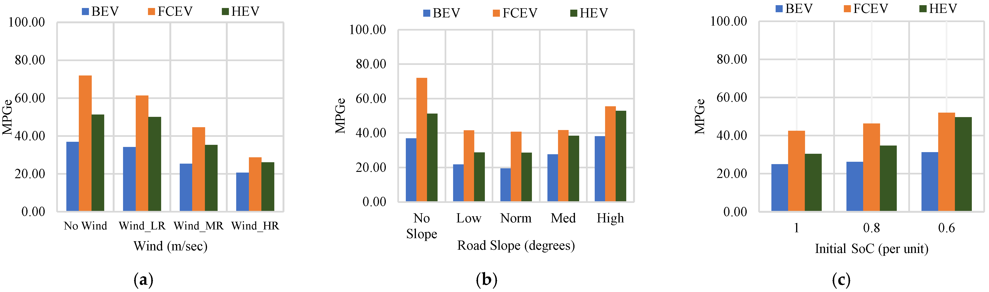
3. Methodology and System Description

This section details the main study boundaries, the considered scenarios, the various parameters, and the methodology of this paper. First, the main parameters of the case studies are discussed in Section 3.1, and then the explored scenarios are presented; the varied wind and road conditions are discussed in Section 3.2.

This paper focuses primarily on microlevel efficiency analysis of three EVs with different configurations for a specific road trip. The workflow shown in Figure 1c is divided into two main phases: phase one represents all simulations carried out on the vehicles, and phase two encompasses the analysis part, using MATLAB Simulink as a simulation environment. As depicted from the workflow in Figure 1c, the vehicles are all tested based on the standardized FTP-75 driving cycle profile, such that their performance for the whole journey is analyzed under varying trip factors for weather, road gradients, and initial SoC. These factors are examined individually and cumulatively such that a total of 39 scenarios is simulated for each vehicle. Using a comprehensive sensitivity analysis that represents all the possible combinations of these configurations and variables, the three-vehicle performance is analyzed. The second phase of the workflow is divided into (a) comparative analysis and (b) prediction. In the comparative analysis section, vehicle performance is analyzed and compared across three key metrics—energy consumption, powertrain efficiency, and emissions—in an attempt to find the most efficient and balanced configuration among BEVs, FCEVs, and HEVs under varying trip conditions. For the prediction section, a more generalized model is developed based on statistical analysis and regression to estimate vehicle performance across different driving conditions, environmental variables, and untested scenarios.

3.1. Electric Drive Train Description

This paper provides a comprehensive analysis considering three EV configurations:

(1)

Case 1: Battery-only EV (BEV);

(2)

Case 2: Fuel Cell EV (FCEV);

(3)

Case 3: Hybrid EV with Battery and Fuel Cell Energy Sources (HEV).

In the context of this research, the configuration where the power split is equal is referred to as an HEV. Performance analysis for BEVs, FCEVs, and HEVs is carried out under three initial SoC scenarios (100%, 80%, and 60%, respectively). The BEV may be considered the baseline configuration as it is the most mature and widespread technology. Figure 1 shows the main features of the three distinct EV configurations that are discussed for analysis, with the paper workflow in Figure 1c. For a fair comparison, there are shared parameters among all studied cases, which are listed in

Table 2. The main features and simulation boundaries of the EV.

Parameter	Value	Unit
Vehicle Weight	1500	kg
Vehicle Frontal Area	2.81	m2
Vehicle Drag Coefficient	0.29	-
Motor Rated Current	200	A
Motor Rated Voltage	650	V
Motor Peak Speed	20,000	rpm
Motor Peak Torque	600	Nm
Motor Peak Power	300	kW

and

Table 3. Main energy storage parameters of EVs.

Parameter	Case 1: BEV	Case 2: FCEV	Case 3: HEV
Battery Ampacity (Ah) at 100% SoC	53.1	2.5	53.1
Battery Pack Voltage at 100% SoC	303.9	303.9	303.9
Battery Capacity (kWh) at 100% SoC	15.9	0.75	15.9
Battery Peak Power (kW) at 100% SoC	80.7	3.8	80.7
Number of Cells	N/A	400	400
Voltage per Cell (V)	N/A	1.225	1.225
Exchange Current Density (A/cm2)	N/A	8.24 × 10−5	8.24 × 10−5
Maximum Current Density (A/cm2)	N/A	1.4	1.4
Active Area per Cell (cm2)	N/A	280.0	280.0
Peak Voltage (V)	N/A	490.0	490.0
Peak Current (A)	N/A	392.0	392.0
Peak Power Output (kW)	N/A	192.0	192.0
Voltage per Cell (V)	N/A	1.225	1.225

N/A: Not Available

.

Figure 1. Electric vehicle configurations: (a) System description, (b) EV free body model, (c) workflow.

Figure 1. Electric vehicle configurations: (a) System description, (b) EV free body model, (c) workflow.

3.1.1. Vehicle Physical Model

Figure 1b shows the EV’s free-body model, where the adopted vehicle modelling approach integrates both mechanical and mathematical principles to describe vehicle behaviour. Road load modelling is widely used in the literature to characterize vehicle dynamics, such that a one-dimensional vehicle model is used to represent the propulsion of the vehicle based on fundamental motion equations. The basic forces acting on the vehicle include:

• Aerodynamic drag force ($F_{AD}$);
• Rolling resistance force ($F_{RR}$);
• Gravitational force ($F_G$);
• Acceleration force ($F_A$).

These forces are illustrated in Figure 1b, and the total traction force ($F_{\mathrm{T}}$) required to move the vehicle is given by

$$F_{\mathrm{T}}=F_A+F_G+F_{RR}+F_{AD}$$

(1)

The acceleration force is the force required to accelerate the vehicle and is expressed as

$$F_A=m\cdot a$$

(2)

where

• m is the vehicle mass (kg);
• a is the acceleration (m/s²).

The sign of $F_A$ depends on the direction of acceleration. It is positive during acceleration and negative when decelerating (braking).

The gravitational force component along an inclined road is

$$F_G=m\cdot g\cdot sin\left(\theta \right)$$

(3)

where

• g is the acceleration due to gravity (9.81 m/s²).
• θ is the road inclination angle (degrees).

When the vehicle moves uphill, sin (θ) is positive, thus increasing the required traction force. If it is moving downhill, then sin (θ) is negative, reducing the force needed and potentially operating in regenerative braking mode.

The rolling resistance is caused by tyre deformation and road contact. It is expressed as

$$F_{RR}=C_r\cdot m\cdot g\cdot cos\left(\theta \right)$$

(4)

where

• $C_r$ is the rolling resistance coefficient (typically 0.01–0.02 for cars).
• $cos\left(\theta \right)$ accounts for the effect of the incline.

Rolling resistance opposes motion and is always present regardless of vehicle movement direction.

Aerodynamic drag force opposes vehicle motion due to air resistance:

$$F_{AD}={\displaystyle \frac{1}{2}}{C}_d\cdot \rho \cdot A_F\cdot { (v-v_{wind})}^2$$

(5)

where

• $C_d$ is the aerodynamic drag coefficient (typically 0.2–0.4).
• $\rho$ is the air density equivalent to 1.2 (kg/${\mathrm{m}}^3$).
• $A_F$ is the frontal area of the vehicle in $\left({\mathrm{m}}^2\right)$;
• $v$ is the vehicle velocity in (m/s).
• $v_{wind}$ is the wind speed component in the direction of travel (m/s).

If the wind is a headwind (blowing against the vehicle), then $v_{wind}$ is positive. If the wind is a tailwind (blowing in the same direction), then $v_{wind}$ is negative. In this paper, all winds are assumed to be headwind, thus opposing the vehicle. The drag force increases quadratically with speed, meaning that higher speeds result in significantly greater aerodynamic resistance.

Total traction force (F_T) can be calculated by combining all the forces acting on the vehicle:

$$F_{\mathrm{T}}=m\cdot a+m\cdot g\cdot sin\left(\theta \right)+C_r\cdot m\cdot g\cdot cos\left(\theta \right)+{\displaystyle \frac{1}{2}}{C}_d\cdot \rho \cdot A_F\cdot { (v-v_{wind})}^2$$

(6)

This equation serves as the foundation for analyzing vehicle performance, energy consumption, and powertrain efficiency.

Then, this force is used to calculate the torque and power required from the electric motor based on the following steps:

Torque is calculated as

$$T=F_{\mathrm{T}}\cdot r_{\mathrm{w}}$$

(7)

where

• T is the torque (Nm);
• $r_{\mathrm{w}}$ is the effective wheel radius (m).

The rotational power is given by

$$P_{\mathrm{m}\mathrm{e}\mathrm{c}\mathrm{h}}=T\cdot \omega$$

(8)

where

• $P_{\mathrm{m}\mathrm{e}\mathrm{c}\mathrm{h}}$ is the mechanical power (W).
• ω is the angular velocity of the wheel (rad/s).

The angular velocity ω is related to the vehicle speed:

$$\omega ={\displaystyle \frac{v}{r_{\mathrm{w}}}}$$

(9)

Thus, substitute ω into the following power equations:

$$P_{\mathrm{m}\mathrm{e}\mathrm{c}\mathrm{h}}=F_{\mathrm{T}}\cdot r_{\mathrm{w}}\cdot {\displaystyle \frac{v}{r_{\mathrm{w}}}}$$

(10)

$$P_{\mathrm{m}\mathrm{e}\mathrm{c}\mathrm{h}}=F_{\mathrm{T}}\cdot v$$

(11)

This is the mechanical power required to drive the wheels. Then, the electric motor power input depends on efficiency:

$$P_{\mathrm{m}\mathrm{o}\mathrm{t}\mathrm{o}\mathrm{r}}={\displaystyle \frac{P_{\mathrm{m}\mathrm{e}\mathrm{c}\mathrm{h}}}{\eta }}$$

(12)

where

• η is the motor efficiency.

3.1.2. Drive Train Specifications and Case Studies Description

As mentioned earlier, all simulations carried out in this work were conducted using MATLAB Simulink to model the vehicle dynamics and evaluate performance metrics across the defined scenarios, given the main features and simulation boundaries of the EV, as presented in Table 2. To ensure a meaningful evaluation of the driving cycle’s impact on the battery’s state of charge (SoC) within a manageable simulation time, the total battery capacity was intentionally scaled down from standard values. This adjustment allows the simulation to demonstrate the SoC variations more effectively, as a full-scale battery would require significantly longer driving distances to exhibit comparable changes. With a vehicle weight of 1500 kg and a frontal area of 2.81 m², the aerodynamic efficiency of the EV is influenced by its drag coefficient of 0.29, which represents the resistance of the vehicle to airflow.

These factors determine the energy consumption necessary to overcome the rolling resistance and aerodynamic forces as the vehicle moves. The motor specifications include a peak output power of 300 kW, a peak torque of 600 Nm, and a maximum rotational speed of 20,000 rpm. Additionally, the motor is designed for efficient power delivery while maintaining operational stability with a rated voltage of 650 V and current of 200 A. The performance chart of the electric motor employed in the electric vehicle is depicted in Figure 2, including its speed‒torque profile and motor efficiency map. These parameters were constant across the three EV configurations.

The storage parameters of EVs are responsible for determining the performance, range, and lifespan of an energy storage system in an electric vehicle. Table 3 provides information about the storage parameters of the EVs. In Case 1 (BEV) and Case 3 (Hybrid EV), the battery has a capacity of 15.9 kWh, a voltage of 303.9 V, and an ampacity of 53.1 Ah, indicating that both configurations rely significantly on battery storage. However, in Case 2 (FCEV), since the primary energy source is the fuel cell stack, the battery capacity is significantly lower (0.75 kWh, 2.5 Ah).

For the fuel cell-based configurations (Cases 2 and 3), additional fuel cell parameters are provided. With 1.225 V per cell, the fuel cell stack consists of 400 cells in both cases, resulting in a peak voltage and current of 490 V and 392 A, respectively. This setup enables a peak power output of 192 kW, thus providing substantial energy support. The exchange and maximum current densities are 8.24 × 10⁻⁵ A/cm² and 1.4 A/cm², respectively, with an active area per cell of 280 cm², highlighting the electrochemical efficiency of the system. The hybrid case (Case 3) benefits from both battery and fuel cell contributions.

3.2. Operational and Environmental Parameters

The objective of this analysis is to provide a unified comparison of the performance of different EV configurations under realistic conditions, which involves considering diverse external parameters. Accordingly, this section provides details of the operational and environmental parameters that will be incorporated in this study to identify the most efficient configuration among the three tested vehicles by analyzing key parameters such as energy consumption, driving range, and adaptability to varying road and climate conditions, as described in Section 4 and Section 5.

3.2.1. Operational Parameters

These parameters represent the way the vehicle is driven and operated. Typically, EVs are tested under standard driving cycles such as WLTP, NEDC, and FTP-75, which represent urban, highway, and mixed roads, respectively, or with real-time-based driving data for a portion of the road. Standardized performance evaluation is crucial for fair comparisons and evaluations regardless of personal preferences. For this reason, the FTP-75 driving profile illustrated in Figure 3 is utilized. This driving profile represents varying degrees of driving styles, such as economic and aggressive, and periods of acceleration, deceleration, and sustained speed.

3.2.2. Environmental Parameters

To further improve the testing conditions and add a sense of realism to the driving cycles, varying wind and road slopes are added as parametric studies. In this way, these external factors are reflected in the results, with details of the environmental parameters as follows.

Figure 3. Speed profile and distance over the driving cycle.

Figure 3. Speed profile and distance over the driving cycle.

Road Slope (Gradient)

Road slopes significantly affect EV’s peak power demand, driving cycle, and overall energy consumption. Driving uphill typically requires more torque to maintain the required speed, which increases the demand from the energy source and the drive-train. On the other hand, regenerative braking is possible in downhill driving, which can improve the overall efficiency and battery SoC. In this analysis, four road slope profiles are considered; which are identical in shape but with incremental magnitudes to emulate a wide range of road conditions. The data are based on extracted road slope conditions from central Cairo, which represent urban conditions and moderate road slopes. Then, it moves to the outer regions with more aggressive slopes. This baseline condition is identified in

Table 4. Wind speed and road grade values.

Parameter	Wind Speeds Range
	Low		Moderate		High
Average Wind Speed (m/s)	20.0		40.0		60.0
Minimum Wind Speed (m/s)	0.0		0.0		20.0
Maximum Wind Speed (m/s)	8.8		20.7		37.3
Parameter	Road Slope Range
	Low	Normal		Moderate		High
Average Slope (°)	0.10	0.20		0.41		0.61
Maximum Uphill Slope (°)	2.83	5.65		11.30		16.95
Maximum Downhill Slope (°)	−3.43	−6.87		−13.74		−20.61
Peak to Peak Slope (°)	6.26	12.52		25.04		37.56

and Figure 4b as ‘Normal’, which has maximum road slope angles of 5.65° and −6.87° representing uphill and downhill, respectively. To simulate smoother conditions, the same profile is repeated at half these normal values and labelled ‘Low’; then, after doubling and tripling, the normal values are considered ‘Moderate’ and ‘High’, and specific values are listed in Table 4 and illustrated in Figure 4b. In summary, performance analysis is performed for 4 variations in road slopes (low, normal, moderate, and high), representing a wide range of road severities, thus improving the understanding of EV performance.

Wind Conditions

Based on real-world wind data, three wind profiles representing low, moderate, and high winds are examined, with assumed direction to be headwind, thus representing the hardest scenario. Wind profiles are shown in Figure 4a, with details listed in Table 4.

Figure 4. Wind speeds and road grade profiles: (a) wind speed, (b) road slope.

Figure 4. Wind speeds and road grade profiles: (a) wind speed, (b) road slope.

3.3. Case Studies and Performance Metrics

As discussed earlier, three EV configurations are under study, namely, BEVs, FCEVs and HEVs, and this represents the major comparative part of the analysis. The three main variables are the initial SoC, road slope, and wind speed. A multivariable sensitivity analysis is performed, which represents all the possible combinations of these configurations and variables. Specifically, three wind speed ranges, four road slope conditions, and three initial SoC values are explored; thus, for each configuration, 36 different scenarios are explored. In addition to these 36 scenarios, three baseline conditions are also considered, which represent zero wind speed and zero road slope at 100%, 80%, and 60% initial SoCs. Thus, a total of 39 variations are simulated for each EV configuration, with all simulations executed via an elaborate model in the MATLAB Simulink environment. The data are then collected, processed, and evaluated, as discussed in Section 4 and Section 5.

Since the main scope of this work is focused on evaluating the effect of external factors on system-level vehicle performance, the modelling approach incorporates battery and motor efficiency into account while neglecting energy losses associated with internal elements such as auxiliaries, power electronic units, and transmission system components [34]. Nevertheless, such losses typically represent a minor portion of total energy consumption, with typical values of 5–8% of overall energy use under standard driving conditions for auxiliary systems and a value of 5% or less for the transmission system [35,36]. As for converter losses, they are often simplified or assumed to be ideal in sensitivity studies [37]. While the analysis carried out in this work uses a model with neglected auxiliaries, transmission, and converter losses to prioritize comparative analysis and computational feasibility of 117 simulated cases, it is worth noting that the magnitude for such losses remains within acceptable bounds and would affect all compared vehicles similarly.

To create a unified framework for comparing the three vehicles, a comparative metric analysis is constructed, which divides the areas of comparison into three main categories: (a) energy, (b) powertrain performance, and (c) environmental impact metrics, as depicted in Figure 1b. This structured approach enables comparison and assessment of the three vehicle types under a variety of conditions, including weather variability, road gradients, and different initial SoCs.

4. Results

This section presents the results obtained from running several simulation experiments on BEVs, FCEVs, and HEVs via the model described in Section 3. The results are divided into three major subsections. The first subsection relates to the energy and efficiency performance parameters, the second section addresses the powertrain performance, and the third section presents the main environmental impacts of the analysis.

4.1. Energy Performance

In this part, vehicles are compared in terms of energy utilization under different driving conditions of weather, roads, and SoCs, providing a better understanding of how efficiently each vehicle type converts stored energy into propulsion under the influence of external factors such as wind, road slopes, and battery initial SoCs. In addition, under this category, factors such as energy per distance, total net energy, battery energy discharge, and the FC/battery energy ratio are evaluated for comparison, as indicated in Figure 5, Figure 6, Figure 7 and Figure 8.

4.1.1. Total Net Energy

With respect to the total net energy in the battery and fuel cell, this metric represents the overall energy consumed during the whole drive cycle and is regarded as a complementary metric with energy per distance, as it provides a broader perspective on the vehicle’s total energy usage over a given journey. It is clear from Figure 5a–c that wind resistance and road slopes are the most influential factors affecting total net energy consumption, whereas minimal effects are exhibited due to the initial SoC. Higher initial SoC levels improve efficiency, underscoring the importance of effective battery management. Compared with FCEVs and HEVs, BEVs have higher total energy usage, which benefits from fuel cell and hybrid energy management.

Figure 5. Total net energy variations: (a) wind speed, (b) road slope, (c) initial SoC.

Figure 5. Total net energy variations: (a) wind speed, (b) road slope, (c) initial SoC.

4.1.2. Energy Consumption per Distance

Figure 6a–c shows the influence of environmental factors (wind), road slopes, and initial SoC on energy per distance. As shown in Figure 6, energy consumption per distance is affected primarily by weather conditions and the road slope, with a minimum effect due to the initial SoC and following the same trend as the total net energy. In terms of vehicle performance, BEVs are the most affected by consuming the most energy under high-wind conditions compared with FCEVs and HEVs. Compared with that with no wind effect, the percentage increase in energy per distance due to wind resistance is greater for BEVs, accounting for 72.25%, followed by HEVs, with an increase of 69.82%, and FCEVs, with an increase of 68.21%. This is due to the total reliance of BEVs on battery power, making them more susceptible to efficiency drops under aerodynamic drag, whereas for FCEVs and HEVs, a lower energy demand increase is exhibited because of their reliance on alternative energy sources.

Similarly, the road gradient increases energy consumption as the road inclination increases, where the impact is mostly exhibited in BEVs, followed by FCEVs, and HEVs are the lowest, as they can alternatively switch between resources effectively. This translates into a 63.1% energy consumption per distance increase in BEVs, followed by a 59.85% increase with HEVs, and finally, a 59.33% increase in the FCEV case.

In terms of the influence of the initial SoC, the trends in Figure 6 are relatively stable across all vehicles, indicating that the initial SoC does not have a direct effect on energy efficiency per distance if a sufficient charge is available. However, it is worth noting that the HEV is the most affected in that case, as when the SoC is low, the FC tries to compensate for its energy requirements, leading to higher energy consumption by relying more on hydrogen power. In contrast, SoC does not affect the FC, which relies solely on the FC for powering its needs.

Figure 6. Energy per distance variation: (a) wind speed, (b) road slope, (c) initial SoC.

Figure 6. Energy per distance variation: (a) wind speed, (b) road slope, (c) initial SoC.

4.1.3. Miles per Gallon Equivalent

Miles per gallon equivalent (MPGe) is a standardized comparison metric and represents how far a vehicle can travel using the energy equivalent of one gallon of gasoline. The higher the MPGE is, the less energy is required per mile, and the more efficient the drive train is. As shown in Figure 7, MPGe is negatively impacted by the wind speed and road slope, requiring more energy to overcome the air drag resistance and gravitational force. On the other hand, energy recovery is maintained with regenerative braking at high slopes, which slightly improves MPGe performance in BEVs and HEVs. In terms of the effect of the initial SoC, the MPGe slightly increases as the initial SoC decreases. Conclusively, the FCEV performs better among all three vehicles in terms of showing the lowest efficiency drop, whereas the lowest efficiency drop is achieved by the BEV.

Figure 7. MPGE variation: (a) wind speed, (b) road slope, (c) initial SoC.

Figure 7. MPGE variation: (a) wind speed, (b) road slope, (c) initial SoC.

4.2. Powertrain Performance

For the powertrain performance assessment, this section evaluates the motor and battery system for the three vehicles studied by examining the efficiency, motor, battery, and FC performance for the whole driving cycle.

4.2.1. Efficiency

The efficiency map of the motor equipped with the three vehicles is shown in Figure 8, in addition to the torque/speed operating points. This represents the motor’s operating conditions during different driving scenarios. The optimal operating range is the range of speed and torque where the motor performs most efficiently, which is crucial for optimizing performance and energy consumption. As seen from the efficiency map and

Table 5. Summary of the operating ranges of the motor efficiency, speed, and torque.

	BEV	FCEV	HEV
Efficiency (%)	~85–88%	~85–91%	~89–94%
Speed range (rpm)	~(775–1062)	~(887–1251)	~(826–1192)
Torque range (Nm)	~(15.35–78.14)	~(26.8–85.9)	~(25.2–87.4)

, the BEV operational points are clustered mainly in the speed range of 775–1250 rpm and positioned in the lower efficiency zone. This suggests that the vehicle operates at lower efficiency values, particularly in low-speed, high-torque regions. Moderate efficiency is observed in all operating ranges of FCEVs, which are positioned at a slightly higher speed range and efficiency than BEVs (between 887 rpm and 1251 rpm). For HEVs, higher efficiency is achieved with slightly less speed variation than for FCEVs. It can be concluded that HEVs are the highest among all three vehicles in terms of efficiency, followed by FCEVs and BEVs. In terms of torque variations, for the three vehicles, the highest variability is achieved for BEVs, followed by FCEVs and HEVs. This could indicate that BEVs experience more torque variations during a trip because of their full reliance on battery power, unlike FCEVs and HEVs, which rely on fuel cells and batteries, leading to a better load distribution.

Figure 8. Efficiency map and speed/torque operating points.

Figure 8. Efficiency map and speed/torque operating points.

4.2.2. Motor Performance

Figure 9 provides insight into motor performance throughout the entire driving cycle. The motor current, power, speed, and torque are analyzed for the three vehicles under investigation. With respect to motor current, large spikes are exhibited in BEVs, which are accompanied by high power and torque bursts, indicating their suitability for high acceleration and rapid response. In contrast, FCEVs and HEVs have similar smooth current, motor power and torque responses, which makes them more applicable for long-distance, steady-state driving.

4.2.3. Battery and Fuel Cell Performance

The FC-to-battery energy and power ratios are two key performance metrics since they represent the amount of total long-term energy usage and the instantaneous power supplied by the fuel cell relative to the battery over the trip, respectively [38]. Unlike BEVs, which are fully dependent on the battery system, the energy for propulsion in FCEVs and HEVs comes from two sources: the battery and the fuel cell. Figure 10 shows a stacked column chart for how energy consumption is managed between both sources, where the areas of battery-only operation and areas of dual power source cooperation are demonstrated. For all wind speed conditions, the propulsion energy mainly comes from the fuel cell in the case of the FCEV. In contrast, in the HEV case, higher wind speeds result in more fuel cell operation in the power generation process. Similar effects are observed as the road gradient and initial SoC change, steeper slopes, and lower SoCs drive both FCEVs and HEVs to rely more on the fuel cell, mainly as the prime source for propulsion, due to the increased power demand. Unlike FCEVs, which rely heavily on fuel cells, the energy share is greater in HEVs with more balanced energy management.

The ratio between the battery energy charge and discharge is an important metric utilized to assess vehicle performance. This metric is crucial for improving vehicle range predictions, which affects the planning of EV infrastructure elements and charging station allocation. In Figure 11a–c, the stacked column chart of average battery energy discharging vs. charging is shown for the tested vehicles. A significant increase in energy discharge is noted in Figure 11a for BEVs, indicating that more energy is needed to maintain performance under windy conditions. In contrast, FCEVs and HEVs also increase; however, this increase is less noticeable than that of BEVs. Figure 11b shows that, compared with FCEVs and HEVs, BEVs exhibit a noticeable increase in energy discharge with increasing road slopes. Finally, in Figure 11c, a more noticeable increase in energy discharge for FCEVs and HEVs is noted as the initial SoC increases compared with the consistent energy discharge in BEVs across all initial SoC levels. Conclusively, under varying conditions, BEVs exhibit more significant changes in energy discharge than FCEVs and HEVs.

Figure 10. Average fuel cell energy vs. battery net energy variation: (a) wind speed, (b) road slope, (c) initial SoC.

Figure 10. Average fuel cell energy vs. battery net energy variation: (a) wind speed, (b) road slope, (c) initial SoC.

Figure 11. Average battery energy charge and discharge variations: (a) wind speed, (b) road slope, (c) initial SoC.

Figure 11. Average battery energy charge and discharge variations: (a) wind speed, (b) road slope, (c) initial SoC.

Battery performance throughout the vehicle’s journey can be assessed, as shown in Figure 12, which shows how the SoC changes. High depletion rates are exhibited in BEVs, with a steady drop in battery voltage due to large battery discharge, as observed in Figure 12a,b. In addition, high battery power fluctuations and high current spikes are experienced, especially in driving mode, as shown in Figure 12c,d. In contrast, moderate depletion is exhibited by the FCEV because of the slight battery voltage drop and moderate power and current. Finally, the lowest current and power demand is achieved in the HEV, accompanied by slow battery depletion and a stable voltage profile.

Analyzing the FC curves, the voltage produced by the fuel cell changes as the driving cycle proceeds, as depicted in Figure 13a. The additional power from the battery causes HEVs to have more stable voltage behaviour than FCEVs. FCEVs’ prime reliance on the fuel cell for power results in greater voltage fluctuations during different driving conditions. Figure 13b shows the current responses of the fuel cell vs. the driving cycle time. HEVs exhibit more stable current behaviour for the same reason of stable fuel cell voltage, whereas FCEVs experience more significant current fluctuations since they rely solely on the fuel cell, leading to greater current variations during different driving conditions. The hybrid system in HEVs can lead to better overall efficiency and fuel cell longevity by reducing the load on the fuel cell during high-power demand. The variation in fuel cell power in Figure 13c is clearly related to the variation in the fuel cell current, where the HEV exhibits more stable behaviour than the FCEV.

Figure 14 shows the battery, fuel cell, and motor power consumption variations in the three vehicles investigated over the entire driving cycle. Since the battery is the sole source of power for the BEV’s propulsion system, the power consumption of the battery and motor varies significantly with different driving conditions, as shown in Figure 14a. On the other hand, the power consumption of the FC and motor is depicted in Figure 14b, where the fuel cell acts as the primary power source supplying all of the vehicle’s power demands. The fuel cell’s power output fluctuates with driving conditions, similar to the BEV response. Additionally, Figure 14c illustrates how power consumption varies in the battery, fuel cell, and motor over the driving cycle in FCHEVs. With the aid of hybridization, a combination of a fuel cell and battery power guarantees more stable power consumption, leading to smoother variations in power consumption than those of BEVs and FCEVs.

Figure 13. Fuel cell performance parameters: (a) fuel cell voltage, (b) fuel cell current, (c) fuel cell power.

Figure 13. Fuel cell performance parameters: (a) fuel cell voltage, (b) fuel cell current, (c) fuel cell power.

Figure 14. Power consumed (kW): (a) BEV, (b) FCEV, (c) HEV.

Figure 14. Power consumed (kW): (a) BEV, (b) FCEV, (c) HEV.

4.3. Environmental Metrics

CO₂ emission calculation is an important metric for environmental sustainability and a core objective for sustainable transportation [39]. By measuring the amount of CO₂ kg emissions, the three vehicles were compared, taking into account the effects of the battery’s state of charge, road slope, and external wind conditions. As per Figure 15 and the parallel plots of Figure 16, it is clear that the wind speed and road conditions affect emissions, particularly for BEVs and FCEVs, because of the increased energy consumption to overcome wind air resistance and uphill driving. On the other hand, the emissions remain relatively constant with varying initial SoCs, indicating that the battery’s initial state has less impact on CO₂ emissions. A comparison of all three vehicles clearly reveals that FCEVs have the lowest CO₂ emissions among the three vehicle types, followed by HEVs and BEVs, with the highest CO₂ emissions compared with those of the other two vehicle types across all trip-varying conditions.

5. Discussion

As demonstrated in Section 4, this paper presents a comparative study of BEVs, FCEVs, and HEVs via a simulated modelling approach, integrating real-world weather data and driving cycles via actual road data with frequent stops, intersections, and varying driving styles (eco and aggressive). Vehicles are assessed via a multicriteria assessment metric system that compares the three vehicles in terms of energy and efficiency, powertrain performance, and emissions. This metric system has been structured to examine the effects of weather conditions (low to high winds), road gradients (low to high slopes), and different initial SoCs on vehicle performance in both individual and cumulative manners.

Section 5.1 is provided to evaluate each vehicle’s overall performance and sustainability, thus providing more insights for evaluating vehicle performance in a more holistic, qualitative manner by consolidating all previously discussed metrics. In addition, a more generalized methodology involving correlation and regression analysis is carried out in Section 5.2 and Section 5.3 to quantify the impacts of the initial state of charge, road grade, and wind speed on energy consumption and performance. This helps provide a more structured predictive approach for analyzing unexplored driving scenarios in a systematic manner, allowing for better data-driven decision-making with respect to EV power evaluation, environmental sustainability, and fleet management.

5.1. Overall Vehicle Performance Evaluation

Table 6. Comparative evaluation of BEVs, FCEVs, and HEVs.

Metric	BEV	FCEV	HEV
Energy Utilization	Low	Moderate	High
Net Energy Saving	Low	Moderate	High
MPGe	Low	High	Moderate
Efficiency	Moderate	Moderate–High	High
Speed Range	Moderate	Moderate–High	High
Torque Range	Moderate	High	High
Motor Performance	Moderate	Moderate	High
Energy Distribution	Low	Moderate	High
Power Energy Characteristics	Low	High	Moderate
Carbon Neutrality	Low	High	Moderate

compares the three vehicles via the multiple key metrics explained in Section 4, which utilize a qualitative scale and four comparative levels to indicate relative performance, namely, low, moderate, moderate-high, and high. Consequently, Table 6 highlights the strengths and weaknesses of each vehicle technology across the studied areas. Furthermore, the radar plot in Figure 17 provides a better visual representation of the benefits and limitations of each configuration. With respect to the evaluation of BEVs, their moderate motor and torque capabilities may slightly compensate for their overall low performance, making them ideal for rapid and dynamic urban driving where more regenerative braking action can assist in recovering some of the lost energy. Long-distance driving is still a major concern, raising more doubts regarding range anxiety and the need for more reliable and robust charging stations. Its low energy utilization is reflected by high total net energy and low MPGe, resulting in higher energy consumption over the entire drive cycle. Consequently, this is further reflected in the vehicle’s overall efficiency, making it less efficient than other vehicle technologies. In addition, since they are fully battery dependent, BEVs have low energy distribution flexibility, which may be translated into a limited driving range and long charging times. Furthermore, its low degree of carbon neutrality indicates that BEV emissions have a highly negative environmental effect.

A more balanced performance across all metrics is demonstrated by FCEV performance, offering a moderate to high overall status. Compared with BEVs, their better energy consumption pattern, MPGe, and net energy savings indicate a promising distance-to-energy ratio and energy efficiency, making them well suited for long trips on highway roads. In addition, their strong powertrain response due to fuel cell utilization is evidenced by their high-power characteristics and torque range, particularly under varying load and trip conditions. Their reliance on a double-power propulsion system increases their flexibility in energy distribution. Moreover, their highest carbon neutrality score highlights their potential for zero-emission operation when they are operated with green hydrogen. However, despite their ability to deliver a smooth and dependable powertrain response, they do not possess the immediate torque and seamless power delivery that BEVs possess.

HEVs, meanwhile, demonstrate the highest among the three configurations as the best compromise among all covered metrics by combining the benefits of both BEVs and FCEVs. With an overall moderate to high score, HEVs are the most energy-efficient option in terms of achieving the best energy consumption per distance travelled and total net energy savings. Because they are able to operate both battery and fuel cells, this hybridization allows them to optimize and balance the energy distribution and offer a high torque range, making them strong powertrains suitable for both urban and highway roads. Although HEVs do not achieve full zero-emission operation, their high motor efficiency and ability to recover energy through regenerative braking make them a practical transition solution toward full electrification.

Figure 17. Radar plot comparing overall BEV, FCEV, and HEV performance.

Figure 17. Radar plot comparing overall BEV, FCEV, and HEV performance.

5.2. Statistical Analysis

In

Table 7. Correlation analysis of the main factors.

	Key Predictors
Response	Initial SoC			Road Grade (°)			Wind Speed (m/s)
	BEV	FCEV	HEV	BEV	FCEV	HEV	BEV	FCEV	HEV
Batt SoC Final	0.798	0.171	0.956	−0.19	−0.302	−0.064	−0.59	−0.829	−0.288
Batt Net Energy (kWh)	0.048	0.983	0.498	0.334	0.055	0.193	0.976	0.152	0.856
FC Energy (kWh)	N/A	−0.08	−0.24	N/A	0.362	0.371	N/A	0.973	0.943
Total Net Energy (kWh)	0.048	0.003	0.097	0.334	0.363	0.315	0.976	0.976	0.978
Energy per Distance (Wh/km)	0.048	0.003	0.097	0.334	0.363	0.315	0.976	0.976	0.978
Grid Carbon Intensity (gCO2/kWh)	0.132	0.717	0.843	0.106	−0.307	−0.338	−0.093	−0.575	−0.292

N/A: Not available, Color Map: Green (+1) → White (0) → Red (−1)

, a correlation analysis is performed, taking into account four main variations, such as the EV configuration, initial SoC, road grade, and average wind speed, while measuring their correlation to some of the main performance metrics. Specifically, the battery’s final SoC is measured along with the battery’s net energy, FC energy, total net energy, energy per distance, and carbon intensity.

For this paper, the Pearson correlation coefficient measures the strength and direction of the linear relationship between two variables, X and Y. In this case, X represent the state of charge, road grade angle, and wind speed, and Y represent various performance metrics as listed in Table 7.

$$r={\displaystyle \frac{\sum (X_i-\overline{X})(Y_i-\overline{Y})}{\sqrt{{\sum (X_i-\overline{X})}^2} ·\sqrt{{\sum (Y_i-\overline{Y})}^2}}}$$

(13)

where

• X_i, Y_i represent individual data points;
• $\overline{X}, \overline{Y}$ represent the mean of X and Y, respectively.
• r ranges from −1 (perfect negative correlation) to +1 (perfect positive correlation), with 0 indicating no correlation.

All three EV configurations show a relatively strong linear relationship between their initial and final SoCs, especially for BEVs at 0.798 and HEVs, where the correlation coefficient is almost equal to 1 (0.956). This means that a high initial charge helps preserve battery charge levels while making the batteries very efficient. In contrast, in FCEVs, the initial charge level appears to have much less influence on the final SoC (0.173). Indeed, for FCEVs, the final SoC is influenced mostly by the wind speed and road grade.

It is evident that road grade specifications significantly impact fuel cell power consumption. In accordance with the correlation analysis, a moderate correlation is exhibited (0.362 for FCEVs; 0.371 for HEVs), primarily due to increased energy requirements in ascending regions. In contrast, BEVs show a weaker correlation (0.334) between the road grade and the total energy consumption. This indicates that regenerative braking is more prominent in HEVs since the energy demand can be split among multiple energy sources. The relatively strong negative correlation between grid carbon intensity and road grade (−0.307 for FCEVs, −0.338 for HEVs) suggests that vehicles operating in hilly terrains tend to decrease energy efficiency and carbon emissions per unit of energy drawn from the grid.

The effect of the average wind speed is also substantial, with a strong negative correlation (−0.829 in FCEV, −0.288 in HEV) for the final battery SoC, indicating that higher wind speeds tend to deplete the battery more quickly. Moreover, as fuel cell energy consumption in FCEVs and HEVs appears very high, a strong positive relationship is exhibited with the speed of wind (0.973 and 0.943, respectively), confirming the increased energy demand for overcoming aerodynamic drag. However, in the case of BEVs, the correlation between the wind speed and the carbon equivalence factor is almost absent (−0.093), probably indicating that energy consumption is very stable even during the variation in winds because the fuel cells do not operate during the entire trip.

5.3. Regression Models

In Section 5.2, statistical analysis was carried out as an initial stage, which helped identify relationships and associations among variables. This helped identify the most influential factors (among the initial Soc, road grade, and wind speed) affecting vehicle performance and emissions for each vehicle type. In addition, this correlational analysis aids in identifying how varying environmental and operational conditions affect each vehicle configuration.

Consequently, regression analysis is conducted in this subsection to quantify the degree of influence of the aforementioned factors on energy consumption and emissions, thus allowing for a more generic and precise estimation of vehicle performance under unexplored conditions.

The required performance metric is modelled using the three main variables considered in a multiple linear regression problem, and the equation can be defined as follows:

$$Y=b_0+b_1 X_1+b_2 X_2+b_3 X_3$$

(14)

where

$X_1, X_2, X_3$ are the independent variables. In this case, they are the initial SoC, wind speed, and road grade.

• $Y$ is the performance metric to be calculated.
• ${b_0, b}_1, b_2, b_3$ are the coefficients of the regression equation indicating the effect of each variable on Y.

To find the regression coefficients, the least-squares method is used, solving the following equation:

$$\mathit{B}={\left({\mathit{X}}^{\mathit{T}}\mathit{X}\right)}^{-1} {\mathit{X}}^{\mathit{T}}\mathit{Y}$$

(15)

where

• X is the design matrix such that

$$\mathit{X}=\left[\begin{array}{c}\begin{array}{cc}1& X_{11}\\ 1& X_{21}\\ 1& X_{31}\end{array} \begin{array}{cc}{X}_{12}& X_{13}\\ X_{22}& X_{23}\\ X_{23}& X_{33}\end{array}\\ \begin{array}{cc}⋮& ⋮ \end{array} \begin{array}{cc}⋮ & ⋮\end{array} \\ \begin{array}{cc}1& X_{n1}\end{array} \begin{array}{cc}{X}_{n2}& X_{n3}\end{array}\end{array}\right]$$

(16)

• Y is the output vector for the performance metrics such as

$$\mathit{Y}=\left[\begin{array}{c}\begin{array}{c}{Y}_1\\ Y_2\\ Y_3\end{array}\\ ⋮\\ Y_n\end{array}\right]$$

(17)

• B is the coefficient vector:

$$\mathit{B}=\left[\begin{array}{c}\begin{array}{c}{\mathit{B}}_1\\ {\mathit{B}}_2\\ {\mathit{B}}_3\end{array}\\ ⋮\\ {\mathit{B}}_{\mathit{n}}\end{array}\right]$$

(18)

• ${\mathit{X}}^{\mathit{T}}$ is the transpose of X.

After obtaining the regression equation, it is crucial to find the coefficient of determination R², which measures how well the model explains Y:

$$R^2=1-{\displaystyle \frac{\sum {(Y_i-\widehat{Y})}^2}{\sum {(Y_i-\overline{Y})}^2 }}$$

(19)

where

• $\widehat{Y}$ is the predicted value.
• $\overline{Y}$ is the mean of Y.

Accordingly,

Table 8. Regression model equations and R² values.

Configuration	BEV	FCEV	HEV	Regression (R-sq) %
Batt SoC Final	9.39 + 64.37 SoC_i − 0.0563 RG − 0.4958 W_avg	−4.45 + 64.37 SoC_i − 0.0563 RG − 0.4958 W_avg	26.31 + 64.37 SoC_i − 0.0563 RG − 0.4958 W_avg	81.39%
Batt Net Energy (kWh)	2.117 + 1.180 SoC_i + 0.00738 RG+ 0.06155 W_avg	−2.023 + 1.180 SoC_i + 0.00738 RG+ 0.06155 W_avg	−0.321 + 1.180 SoC_i + 0.00738 RG+ 0.06155 W_avg	86.29%
FC Energy (kWh)	−0.844 − 0.688 SoC_i + 0.01127 RG+ 0.05762 W_avg	3.015 − 0.688 SoC_i + 0.01127 RG+ 0.05762 W_avg	1.262 − 0.688 SoC_i + 0.01127 RG+ 0.05762 W_avg	89.26%
Total Net Energy (kWh)	1.273 + 0.492 SoC_i + 0.01865 RG+ 0.11917 W_avg	0.992 + 0.492 SoC_i + 0.01865 RG+ 0.11917 W_avg	0.992 + 0.492 SoC_i + 0.01865 RG+ 0.11917 W_avg	97.06%
Energy per Distance (Wh/km)	106.1 + 41.0 SoC_i + 1.554 RG + 9.931 W_avg	82.7 + 41.0 SoC_i + 1.554 RG + 9.931 W_avg	78.4 + 41.0 SoC_i + 1.554 RG + 9.931 W_avg	97.06%
CO2 Intensity (gCO2/kWh)	385.3 + 105.6 SoC_i − 0.442 RG − 0.559 W_avg	−25.7 + 105.6 SoC_i − 0.442 RG − 0.559 W_avg	159.5 + 105.6 SoC_i − 0.442 RG − 0.559 W_avg	98.67%

RG: road grade pk-pk (°); I_SoC_i: initial state of charge; W_avg: average wind speed (m/s).

shows the regression equations and how key parameters influence the battery state of charge, energy consumption, fuel cell usage, and carbon emission intensity across all three vehicle configurations. The high R² values, which range between 81.39% and 98.67%, indicate the model’s strong predictive ability, with a strong explanation of the variations in the dependent variables. Furthermore, these linear models are a major outcome of this analysis, offering a scalable and programmable approach for predicting a vehicle’s performance under unexplored and diverse conditions.

6. Model Validation Analysis Using Commercial EV Models

In this section, the simulation is extended to utilize the battery capacity and power split of three commercial EVs representing the three technologies addressed in this paper, with vehicle specifications listed in

Table 9. Specification of the commercial EV models.

Specification	BEV: Tesla Model 3	FCEV: Toyota Mirai (Gen 2)	HEV: BMW iX5 Hydrogen
Battery Capacity (kWh)	82 kWh	1.24 kWh	20 kWh
Battery Capacity (Ah)	205 Ah	4 Ah	50 Ah
Battery Power (kW)	250+ kW	30 kW	125 kW
Fuel Cell Power (kW)	N/A (Battery Only)	128 kW	125 kW

. In this section, models were tested for two scenarios: (a) a baseline case, representing normal driving conditions, characterized by zero wind speed, flat terrain, and with an initial SoC of 0.6 p.u; (b) an extreme scenario, where vehicles experience the most challenging journey conditions, with the highest wind speeds, roughest road, and same initial SoC as the normal case. Hence, the adverse effects of wind and road conditions can be observed for these commercial EV models compared to normal driving conditions.

The results for SoC profiles over time are summarized in Figure 18 for the three tested vehicle models under both normal and extreme journey conditions. In Figure 18a, it is evidenced that the SoC drop for both BEV and HEV is around 3% for normal conditions, indicating efficient energy usage in mild environments. In contrast, in extreme conditions, the SoC for both vehicles drops significantly to 10% and 14%, respectively, at the end of the drive cycle. This is also reflected in Figure 18b for the battery power consumption with time. Regarding the FCEV, SoC trends of Figure 18c exhibit greater fluctuations compared to the BEV and HEV, with a gradual decrease under normal driving conditions, compared to sharp drops and irregular variations in extreme driving scenarios.

This behaviour can be interpreted due to the different dynamic response characteristics exhibited by the fuel cell, compared to the more stable energy delivery patterns of battery-dominant systems like the BEV and HEV. In Figure 18c, the power split between the battery pack and the FC is illustrated. It shows that the power split is nearly the same for the HEV model and the FCEV; the battery is only used for peak power and acceleration periods and benefits from the regenerative braking.

Figure 18. Commercial EV models result under normal conditions and extreme wind and road grade conditions: (a) battery SoC, (b) battery power, (c) battery and FC power split.

Figure 18. Commercial EV models result under normal conditions and extreme wind and road grade conditions: (a) battery SoC, (b) battery power, (c) battery and FC power split.

Comparing the three modelled vehicles under standard drive cycles for both normal and extreme driving conditions, it can be concluded that although BEVs exhibit the most stable SoC performance with minimal variation and smooth power delivery, their total dependability on battery capacity and recharging demands may often limit their usable range. In contrast, FCEVs demonstrate better potential for extended driving ranges but at the cost of more dynamic SoC behaviour, with noticeable fluctuations due to the transient response characteristics of the fuel cell system, especially under extreme driving. Ultimately, HEVs offer a balanced alternative among all technologies with moderate SoC variations and reasonable energy efficiency, thus placing them as a viable option for mixed driving conditions.

7. Conclusions

EVs offer a promising pathway toward green and more efficient transportation solutions, particularly fuel cell-based solutions. As a result, microlevel efficiency modelling and regression analysis of these vehicles are essential for understanding their energy optimization, performance trade-offs, and environmental impact under varying driving conditions. In this work, the performance of three EVs, including BEVs, FCEVs, and HEVs, was compared via a unified multicriteria framework under a standardized driving cycle while varying the road slope, thus representing different terrains, varying the wind speed profiles for different seasonal effects, and implementing three ranges of initial SoCs. In total, for each EV configuration, 39 scenarios were performed, thus covering a very wide range of operational and environmental conditions.

Compared with other works related to HEVs, this study covers a more comprehensive vehicle performance analysis, covering technical, environmental and predictive measures that have been overlooked in other similar studies. In addition, a thorough and detailed analysis of the results provided valuable insights into the energy consumption, regenerative braking capabilities, drive train limits, and carbon emissions for each case study.

The results revealed that the range and energy consumption are highly affected by the wind speed and terrain conditions. Hence, by including these factors, a more reliable and accurate estimation of the total energy consumption and the driving range is possible. In terms of vehicle performance, FCEVs have an inherently lower refuelling time and lower dependency on lithium-ion batteries; hence, FCEVs can be promising as a sustainable EV solution, assuming green hydrogen production. Among all the tested vehicles, HEVs are the best in terms of efficiency and range in real-world operation, especially when limitations arise against a pure battery electric powertrain. Future studies may also consider evaluating the effects of hydrogen availability, battery degradation, and economic viability on the long-term uptake of these technologies. Awareness of these factors will be instrumental in facilitating the evolution of more sustainable transport solutions.

References

1. International Energy Agency. Global EV Outlook 2024 Moving Towards Increased Affordability. 2024. Available online: https://www.iea.org/reports/global-ev-outlook-2024 (accessed on 1 February 2025).
2. Recalde, A.A.; Lukic, M.; Hebala, A.; Giangrande, P.; Klumpner, C.; Nuzzo, S.; Connor, P.H.; Atkin, J.A.; Bozhko, S.V.; Galea, M. Energy Storage System Selection for Optimal Fuel Consumption of Aircraft Hybrid Electric Taxiing Systems. IEEE Trans. Transp. Electrif. 2021, 7, 1870–1887. [Google Scholar] [CrossRef]
3. Eweda, M.M.; ElNaggar, K. Reinforcement learning for autonomous underwater vehicles (AUVs): Navigating challenges in dynamic and energy-constrained environments. Robot. Integr. Manuf. Control 2024, 1, 31. [Google Scholar] [CrossRef]
4. Hebala, A.; Connor, P.H.; Nuzzo, S.; Gerada, C.; Galea, M. A Holistic Analysis and Experimental Testing of a Passive Heat Path for Electric Motors Slots; IEEE Transactions on Transportation Electrification: New York, NY, USA, 2025; p. 1. [Google Scholar] [CrossRef]
5. International Energy Agency. World Energy Outlook 2024. 2024. Available online: https://www.iea.org/terms (accessed on 1 February 2025).
6. Abo-Khalil, A.G.; Abdelkareem, M.A.; Sayed, E.T.; Maghrabie, H.M.; Radwan, A.; Rezk, H.; Olabi, A. Electric vehicle impact on energy industry, policy, technical barriers, and power systems. Int. J. Thermofluids 2022, 13, 100134. [Google Scholar] [CrossRef]
7. Ibrahim, R.A.; Gaber, I.M. Electric Vehicles: From Charging Infrastructure to Impacts on Utility Grid; IOS Press Ebooks: Amsterdam, The Netherlands, 2024. [Google Scholar] [CrossRef]
8. Rahman, M.; Thill, J.-C. A Comprehensive Survey of the Key Determinants of Electric Vehicle Adoption: Challenges and Opportunities in the Smart City Context. World Electr. Veh. J. 2024, 15, 588. [Google Scholar] [CrossRef]
9. Ibrahim, R.A.; Gaber, I.M.; Zakzouk, N.E. Analysis of multidimensional impacts of electric vehicles penetration in distribution networks. Sci. Rep. 2024, 14, 27854. [Google Scholar] [CrossRef]
10. Christos, T.; Pompodakis, E.E.; Orfanoudakis, G.I. Techno-Economic Feasibility of Fuel Cell Vehicle-to-Grid Fast Frequency Control in Non-Interconnected Islands. Hydrogen 2024, 6, 1. [Google Scholar] [CrossRef]
11. Vengatesan, S.; Jayakumar, A.; Sadasivuni, K.K. FCEV vs. BEV—A short overview on identifying the key contributors to affordable & clean energy (SDG-7). Energy Strategy Rev. 2024, 53, 101380. [Google Scholar] [CrossRef]
12. Mao, T.; Zhang, X.; Zhou, B. Intelligent Energy Management Algorithms for EV-charging Scheduling with Consideration of Multiple EV Charging Modes. Energies 2019, 12, 265. [Google Scholar] [CrossRef]
13. Ragab, A.; Marei, M.I.; Mokhtar, M. Comprehensive Study of Fuel Cell Hybrid Electric Vehicles: Classification, Topologies, and Control System Comparisons. Appl. Sci. 2023, 13, 13057. [Google Scholar] [CrossRef]
14. Asif, U.; Schmidt, K. Fuel Cell Electric Vehicles (FCEV): Policy Advances to Enhance Commercial Success. Sustainability 2021, 13, 5149. [Google Scholar] [CrossRef]
15. Swelam, R.; Khalifa, M.; Mohareb, N.; Moustafa, Y.; Affifi, S. A comprehensive study of travel mode captivity: A nuanced perspective on car captivity in new Cairo, Egypt. Renew. Energy Sustain. Dev. 2024, 10, 16. [Google Scholar] [CrossRef]
16. Al-Ani, S.A.; Dhahir, M.K. Laser-enhanced hydrogen production: Designing a PEC cell photoanode with an exclusive dye material for superior efficiency. Renew. Energy Sustain. Dev. 2024, 10, 407. [Google Scholar] [CrossRef]
17. Xu, Q.; Wu, Z.; Xin, S.; Niu, H.; Zhang, P.; Wang, X. Grid capacity planning model for electric vehicle high charging penetration in power distribution networks. Int. J. Low Carbon Technol. 2025, 20, 279–288. [Google Scholar] [CrossRef]
18. Othman, B.; De Nunzio, G.; Di Domenico, D.; Canudas-De-Wit, C. Ecological Traffic Management: A Review of the Modeling and Control Strategies for Improving Environmental Sustainability of Road Transportation; Elsevier: Amsterdam, The Netherlands, 2019. [Google Scholar] [CrossRef]
19. Fiori, C.; Montanino, M.; Nielsen, S.; Seredynski, M.; Viti, F. Microscopic energy consumption modelling of electric buses: Model development, calibration, and validation. Transp. Res. D Transp. Environ. 2021, 98, 102978. [Google Scholar] [CrossRef]
20. Donkers, A.; Yang, D.; Viktorović, M. Influence of driving style, infrastructure, weather and traffic on electric vehicle performance. Transp. Res. D Transp. Environ. 2020, 88, 102569. [Google Scholar] [CrossRef]
21. Ansari, A.; Abediasl, H.; Shahbakhti, M. Ambient Temperature Effects on Energy Consumption and CO2 Emissions of a Plug-in Hybrid Electric Vehicle. Energies 2024, 17, 3566. [Google Scholar] [CrossRef]
22. Yang, D.; Liu, H.; Li, M.; Xu, H. Data-driven analysis of battery electric vehicle energy consumption under real-world temperature conditions. J. Energy Storage 2023, 72, 108590. [Google Scholar] [CrossRef]
23. Al-Wreikat, Y.; Serrano, C.; Sodré, J.R. Driving behaviour and trip condition effects on the energy consumption of an electric vehicle under real-world driving. Appl. Energy 2021, 297, 117096. [Google Scholar] [CrossRef]
24. Lee, G.; Song, J.; Lim, Y.; Park, S. Energy consumption evaluation of passenger electric vehicle based on ambient temperature under Real-World driving conditions. Energy Convers. Manag. 2024, 306, 118289. [Google Scholar] [CrossRef]
25. Muzir, N.A.Q.; Hasanuzzaman; Selvaraj, J. Modeling and Analyzing the Impact of Different Operating Conditions for Electric and Conventional Vehicles in Malaysia on Energy, Economic, and the Environment. Energies 2023, 16, 5048. [Google Scholar] [CrossRef]
26. Suttakul, P.; Fongsamootr, T.; Wongsapai, W.; Mona, Y.; Poolsawat, K. Energy consumptions and CO2 emissions of different powertrains under real-world driving with various route characteristics. Energy Rep. 2022, 8, 554–561. [Google Scholar] [CrossRef]
27. Jeong, J.W.; Lee, J.; Lee, J.; Cha, J.; Lee, K. Comparison of energy consumption between hybrid and electric vehicles under real-world driving conditions. J. Power Sources 2024, 618, 235190. [Google Scholar] [CrossRef]
28. Tran, T.B.; Kolmanovsky, I.; Biberstein, E.; Makke, O.; Tharayil, M.; Gusikhin, O. Effect of Wind on Electric Vehicle Energy Consumption: Sensitivity Analyses and Implications for Range Estimation and Optimal Routing. ACM J. Auton. Transp. Syst. 2024, 1, 8. [Google Scholar] [CrossRef]
29. Sagaria, S.; Neto, R.C.; Baptista, P. Modelling approach for assessing influential factors for EV energy performance. Sustain. Energy Technol. Assess. 2021, 44, 100984. [Google Scholar] [CrossRef]
30. Miri, I.; Fotouhi, A.; Ewin, N. Electric vehicle energy consumption modelling and estimation—A case study. Int. J. Energy Res. 2021, 45, 501–520. [Google Scholar] [CrossRef]
31. Sagaria, S.; Neto, R.C.; Baptista, P. Assessing the performance of vehicles powered by battery, fuel cell and ultra-capacitor: Application to light-duty vehicles and buses. Energy Convers. Manag. 2021, 229, 113767. [Google Scholar] [CrossRef]
32. Ahn, K.; Rakha, H.A. Developing a Hydrogen Fuel Cell Vehicle (HFCV) Energy Consumption Model for Transportation Applications. Energies 2022, 15, 529. [Google Scholar] [CrossRef]
33. Ahn, K.; Rakha, H.A. Simple Energy Model for Hydrogen Fuel Cell Vehicles: Model Development and Testing. Energies 2024, 17, 6360. [Google Scholar] [CrossRef]
34. Roshandel, E.; Mahmoudi, A.; Kahourzade, S.; Yazdani, A.; Shafiullah, G. Losses in efficiency maps of electric vehicles: An overview. Energies 2021, 14, 7805. [Google Scholar] [CrossRef]
35. Meléndez-Useros, M.; Viadero-Monasterio, F.; Jiménez-Salas, M.; López-Boada, M.J. Static Output-Feedback Path-Tracking Controller Tolerant to Steering Actuator Faults for Distributed Driven Electric Vehicles. World Electr. Veh. J. 2025, 16, 40. [Google Scholar] [CrossRef]
36. Wang, Z.; Qu, X.; Cai, Q.; Chu, F.; Wang, J.; Shi, D. Efficiency Analysis of Electric Vehicles with AMT and Dual-Motor Systems. World Electr. Veh. J. 2024, 15, 182. [Google Scholar] [CrossRef]
37. Fotouhi, A.; Propp, K.; Longo, S.; Auger, D. Simulation for prediction of vehicle efficiency, performance, range and lifetime: A review of current techniques and their applicability to current and future testing standards. In Proceedings of the 5th IET Hybrid. and Electric Vehicles Conference (HEVC 2014), Institution of Engineering and Technology 2014, London, UK, 5–6 November 2014; p. 9.1. [Google Scholar] [CrossRef]
38. Knibbe, R.; Harding, D.; Burton, J.; Cooper, E.; Zadeh, Z.A.; Sagulenko, M.; Meehan, P.A.; Buckley, R. Optimal battery and hydrogen fuel cell sizing in heavy-haul locomotives. J. Energy Storage 2023, 71, 108090. [Google Scholar] [CrossRef]
39. Dulău, L.-I. CO2 Emissions of Battery Electric Vehicles and Hydrogen Fuel Cell Vehicles. Clean. Technol. 2023, 5, 696–712. [Google Scholar] [CrossRef]
Figure 2. Electric motor performance chart: (a) speed-torque profile, (b) efficiency map.
Technologies 13 00150 g002
Figure 9. Motor performance parameters: (a) current, (b) power, (c) speed, (d) torque.
Technologies 13 00150 g009
Figure 12. Battery performance parameters: (a) battery final SoC, (b) battery voltage, (c) battery power, (d) battery current.
Technologies 13 00150 g012
Figure 15. Total CO2 emission variations: (a) wind speed, (b) road slope, (c) initial SoC. CO2 emission: (a) variation with wind speed, (b) variation with road slope, (c) variation with initial SoC.
Technologies 13 00150 g015
Figure 16. Parallel plots for performance comparison of electric vehicle technologies.
Technologies 13 00150 g016