Abstract
Over recent years, location-routing problems have become popular, since they tackle multiple major decisions in supply chains. With the focus now on sustainable supply chains, the problem has become sought-after, with the emphasis on complying with goals set by world leaders such as complying with environmental rules and social equity. As a result, this has opened multiple research directions within the location-routing problem. In the literature, the focus has merely been on two of the sustainability pillars, the environmental and economic pillars, with no integration of the social pillar. In this article, the aim is to integrate the social pillar alongside the environmental and economic ones by modeling the system as a capacitated two-echelon location-routing problem tackling multiple scenarios. Under the umbrella of optimization technology, the algorithm used to solve the problem is a genetic algorithm. This article also demonstrates the process of designing the experimentation phase and selecting variables aiming to fine-tune the models. Multiple parent selection methods and crossover methods were tested, among other variables. The algorithm has proven its success in finding a near-optimum value when compared to the benchmark solution, with an error less than 0.05%. Tournament has performed better as a parent selection method in contrast to stochastic universal sampling, and has proved to be more stable in the face of the stochastic noise induced in the models. This study shows that the social pillar, like the other two pillars, can be integrated in the location-routing problem at an extensive level, beyond what is normally implemented.
1. Introduction
With the year 2030 now in sight, emphasis on turning conventional supply chains into sustainable ones is at an all-time high. All enterprises, of all sizes, are trying to align their goals with the ones set by world leaders for a more sustainable world as a result of the world being in a critical state [1]. The Sustainable Development Goals (SDGs) stressed by world leaders cover various aspects, from ending world hunger to gender equality. These goals are related to the original classification of sustainability, which has three categories—environmental, economic, and social, or as they are also called, the triple bottom line (TBL) [2]. In addition to the challenges normally faced by the traditional supply chain, such as, but not limited to, cost reduction and complying with market demands, the environmental and social demands of the pillars are also considered as challenges. This has come as a result of increased public awareness on the topic of sustainability, affecting the public’s decision to use an enterprise’s services or products based on goodwill. Whether discussing upstream or downstream areas of supply chains, implementing sustainable practices in these focal areas is a current necessity. One of the problems with such a focus is the location-routing problem.
Already a heavily discussed topic, the emergence of the SDGs has led to the location-routing problem (LRP) being one of the most commonly discussed problems in the literature, since it is the combination of two of the four main supply chain decisions: location and transportation [3]. In a sense, LRP is a variant of the conventional vehicle-routing problem (VRP); the variance comes from the idea that all supply chain decisions, including the aforementioned ones, are interrelated with each other. Hence, tackling only one of the decisions without including the others is somehow infeasible. In this case, location and transportation are significantly interrelated with each other. Transportation is an integral part of all supply chain logistics. It includes the delivery of the finished goods from the enterprise facility to the distribution center, and/or from the distribution centers to their customers [4]. This depends on an enterprise’s business model, whether it has a business-to-business model (B2B) or a business-to-customer model (B2C). In addition, especially for manufacturing enterprises, efficient routes from the facility location to distribute the goods is a major problem since the aim is to reduce operational costs and the total cost of investment [4]. This shows the importance of determining the location of the facility early on to serve the enterprise’s allocated budget.
A very common variation of the conventional LRP is the capacitated LRP (CLRP), where the facilities, depots, vehicles used, and customers are all assigned a value for capacity. The CLRP represents a more realistic approach to real-life logistics, since the problem has now become more complex. For facilities, capacity is the production capability of the facility, while for depots, it is its storage capability. For vehicles, it is the weight that can be transported, and for customers, it is the demand value required to be delivered. Uncertainty in CLRP has also been thoroughly discussed in recent years, since market demands have been found to be significantly vulnerable to global events, such as wars and natural disasters. These events deemed the CLRP a stochastic problem in nature. Exact and metaheuristic methods are dominant in the literature for solving different problems regarding CLRP, such as simultaneous pickup and delivery, timed delivery windows, multi-vehicle utilization, etc. These problems directly or indirectly serve the environmental and economic pillars of sustainability. Directly and indirectly mean that the articles in question either clearly state that tackling the LRP aims to achieve more sustainable behavior, or indirectly by simply optimizing the routes and location; this results in sustainable goals being covered.
From both research directions, it is noticeable that there is a lack of inclusion of social pillar factors in the problem itself. This could be affiliated to multiple reasons, including the difficulty of quantifying certain social aspects of sustainability such as health, safety, and corruption, and it was found that most focused on indicators are “job creation”, as in providing jobs for people in the community, and “community development”, as in providing projects to the community, like road construction [5,6,7].
In this article, the aim is to integrate the social pillar alongside the environmental and economic pillars when modeling the LRP. The modeling of the system is performed by solving a two-echelon capacitated location-routing problem (2E-CLRP) using metaheuristic methods in a specific genetic algorithm (GA). The technology is used to determine the location of the main facility and a secondary relay, which suppliers and distribution centers could target for contracting from the available list, the routes taken by assigned vehicles for delivery, and more importantly, the integration of social aspects to consider within the CLRP. Two models were constructed, each tackling a different case: the normal case and the uncertain case. The first model deals with the demand as a static value, while the second model deals with the market demand as a range. The social aspects considered for integration were induced breaks for drivers and the proximity to a transportation hub as monetary penalties which are beyond the topics which are currently being tackled in the literature, namely “job creation” and “community development”. The article also aims to shed light on some details regarding the parameters used in the Genetic Algorithm which seem to be usually overlooked in the literature. This was performed through the fine-tuning of the model, where it was experimented with multiple variables. The remainder of the article is structured as follows: Section 2 is the relevant literature review; Section 3 is the methodology used; Section 4 is the case study section; Section 5 is the experimentation section; Section 6 is the results and discussion section, and finally, Section 7 is the authors’ conclusion and recommendations for future work.
2. Literature Review
2.1. Supply Chain Management
Supply chain management, or SCM, can be defined as the interconnection of the organizations involved in the supply chain. Whether they are the customers or the suppliers, this interconnection is established through upstream and downstream linkages that require coordination between the parties involved. In order to produce a final product or provide a certain service to the consumer, several activities and processes are required to achieve such goals. This is where supply chain management is involved; SCM provides the required tools to enhance the performance of the aforementioned interconnection, hence improving long-term management [8,9]. Supply chain management can be classified into two main categories: traditional supply chain management and modern supply chain management.
2.2. Traditional and Modern Supply Chain Management
- Processes of SCM
There are five SCM processes: planning, sourcing, production, delivery, and return. These five processes are intertwined with each other, and communication between different departments responsible for each process is vital [10].
- Planning:
The planning process involves processes such as business rules, data resources, contracts, compliance, and risk management. For every process involved in planning, a plan element is included. For example, a plan element regarding the delivery is made, including all the necessary information for the commitment of delivery of customers’ orders [10].
- Sourcing:
The sourcing process is responsible for requesting the raw materials required for products or services provided to customers. This task could be directly performed by the main organization, or it could be subcontracted to other companies. These tasks include, but are not limited to, tracking goods throughout their life cycle in the supply chain, scheduling checking, and authorizing suppliers’ payments [10].
- Production:
The production process is dependent on the previous step, where the resources gathered in the sourcing step are used to change them into goods or services that satisfy the customers’ needs. The process normally includes a testing phase, which is repeated multiple times throughout the process to make sure that the product meets the quality and safety standards set by the organization, and more importantly, the governmental bodies responsible for setting these regulations. These tests are performed before mass production and before the product reaches the market. No matter what type of products being produced, these tests are performed on various products, ranging from food products to children’s toys [10].
- Delivery:
The delivery step is a very important step of the supply chain from a logistics perspective since it is responsible for the inventory of goods, the warehouses, how they are managed, and the transportation to and from the previously mentioned warehouses [10].
- Return:
The last process within the supply chain is the return process. This step is affiliated with communicating with sales collection centers to gather information regarding various points, such as the number of sales and returns of products. These returned products can vary from incorrect or defective to unsatisfactory products that require maintenance, repair, and overhauling [10].
Management Strategies
Several strategies utilized for supply chain management have been developed and adopted by different countries and companies around the world. These strategies include, but are not limited to, lean management and total quality management (TQM).
- Lean Management:
Lean management stems from the lean concept, which was first created by Toyota Motor Group in the early 1990s. The main goal of lean management is the optimization of various processes by eliminating and reducing the time spent on non-value-added tasks. These tasks are necessary operations that do not add value to the product, such as transport, waiting, and delays. Within management, it is concerned with identifying and removing waste within the enterprises in the supply chain. Lean management is widely used across major and minor industries [11].
- 2.
- Total Quality Management:
Total quality management shares a lot of the goals and beliefs of lean management regarding the elimination of waste. It is a framework for management that is built on the belief that an organization can achieve long-term success by making sure that all its members, from low-ranking ones to high-level management officials and executives, focus on improving the quality of the products or services provided, and hence deliver on a very important aspect, which is customer satisfaction. Customer satisfaction is a common goal in both total quality management and lean management [12].
To ensure that this quality is achieved, several factors and measures were developed in order to measure the usage of technology from different aspects, since this directly impacts product or service quality.
- Quality of Technology:
This factor is relevant to the type of technology used in production and management activities. For example, using standard data collection techniques such as manual collection is very different from the usage of the capabilities of the Internet of Things. The usage of the Internet of Things in product development, or using big data in the suppliers’ processing, will give the team responsible for the product or service demand the ability to respond faster to fluctuations in demand, which gives the enterprise a competitive advantage [12].
- Quality of Humans:
This factor is concerned with the capability of the human factor in adapting to the technology used. This is absolutely essential for the success and efficiency of the supply chain. The necessity of adaptation of these technologies comes from the nature of this technology, emerging from a very dynamic and a competitive market. Hence, supply chain users and stakeholders must have the necessary skills to use the system and understand their effect and additions to the system [12].
- Quality of Economy:
This factor is used to measure the strength of an enterprise. This is performed by calculating the cost of multiple decisions and their respective alternatives. For example, the usage of new technologies and capable labor may impact the product quality positively, but there might be an increased cost in labor acquisition and technology maintenance [12].
- Quality of Processes:
As previously mentioned, the supply chain can be divided into five main processes: enable, make, source, deliver and return. These processes must be effectively and efficiently operated so that the supply chain becomes successful. This is where quality of processes comes in; several factors are created to evaluate the processes in terms of the following: reliability, repeatability, controllability, and stability. These processes must be applied under similar circumstances and conditions [12].
2.3. Challenges of SCM
Several challenges are easily identified in the implementation of traditional SCM systems: insufficient planning and management of the shipment of goods through the traditional SCM. The traditional SCM has shown its inability to adapt and respond not only to the always growing complexity of the globalization phenomenon, but also to the fluctuating status of the markets, whether domestic or global, which always demands that enterprises compete for the edge in the market [13]. This problem could be specifically associated with the traditional type of SCM, since it does not depend on modern technologies. This is where modern SCMs have a major advantage over traditional ones [14].
One of the strongest challenges in modern SCMs is data management. Data management varies from data cleansing, which removes incomplete information, to interpreting data by using various techniques. The interpretation of data produces useful information, which may be used to achieve a competitive advantage in the market. The second challenge that comes into question is the security and privacy of the information. This has a very negative effect, spanning from affecting the timely delivery of goods from source to destinations to other companies using such information to gain competitive edge over the enterprise [13]. Sharing with suppliers requires information (or a lack of it), and a general mistrust between the members of the entire supply chain is considered as the main barrier in the traditional SCM [14].
2.4. Sustainable Supply Chain Management
Sustainable supply chain management can be defined as the management of various items, such as information, capital flows, and material, not to mention managing interoperability among companies and other stakeholders along the supply chain, while simultaneously taking into consideration all of the three dimensions of sustainable development. It is worth noting that sustainable supply chain management, or SSCM, is an extension of traditional supply chain management which combines both environmental and social issues [15].
The three pillars of sustainability, or the triple bottom line, stipulates that all manufacturing industries and enterprises consider all three aspects thoroughly and simultaneously [16]. The concept is adapted through a model which sets up long-term strategies used by companies that are willing to make the transition from conventional practices to sustainable practices. The transition focuses on the three main pillars of sustainability: environmental quality, social equity, and economic benefits. This research field has a lot of accepted models that describe the three pillars of sustainability and how they overlap with each other, yet the most known and used one is the nested spheres model, which is also known as the Venn diagram explanation. The intersection of all three spheres is where sustainability can be illustrated, as shown in Figure 1 [17].
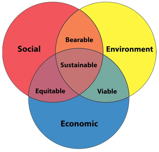
Figure 1.
Venn diagram [18].
Since the scope of this article is on the social pillar of sustainability, an in-depth explanation of the social pillar of sustainability, discussing its challenges, is provided.
2.5. Social Pillar of Sustainability
The social pillar of sustainability refers to the individuals within a specific community. Scholars have concentrated on establishing a definition for sustainability and measuring it using various indicators. Some indicators that may be associated with the social pillar include housing, education, safety and health, fair access to essential services, transportation, recreation, and intergenerational equity. The aim is for future generations not to be disadvantaged by the actions of current and past generations [18]. Numerous definitions of the social pillar of sustainability can be found in the literature. These definitions vary based on the viewpoint and objectives of the organization providing the definition, with several examples outlined below.
The social pillar of sustainability is defined by IUCN WWF, UNEP in 1991 as “development that improves the quality of human life while living within the carrying capacity of supporting ecosystems” [19]. In 1998, Hill defined the social pillar of sustainability as “the preservation of the planet and its ecosystems, society and its communities, for finest, equitable environmental and human health and well-being” [20]. In 1999, Lafferty and Langhelle referred to the social pillar as “A human code of conduct which needs to be achieved in an equitable, inclusive and prudent manner” [21]. In 2000, the World Business Council for Sustainable Development (WBCSD) defined the pillar as “the continuing obligation by business to behave ethically and contribute to economic development while improving the quality of life of the workforce and their families, local community and society at large” [22]. In 2008, Dillard et al. defined the pillar as “social sustainability should be regarded as the process that creates social well-being and health in the present time and also in the future by the efforts of social institutions that facilitate environmental and economic sustainability now and for the future”. The social pillar is regarded in two different dimensions, according to the Organization for Economic Cooperation and development (OECD). The first dimension is the social dimension, which refers to human skills, abilities, knowledge, and talent. The second dimension is the human dimension, which refers to an individual’s performance in the labor market. This was cited by Tracey and Anne in 2008. In 2018, Mani and Delgado concluded that “Social sustainability is all about addressing the social issues in today’s societies, facilitating a sustainable future for the future generations” [18].
Challenges Facing the Social Pillar
As seen from the previous literature, scholars have worked on defining what the social pillar is. Yet, with its importance highlighted, a major challenge has been noticed and highlighted by researchers.
- Undermining of the Social Pillar
Several scholars have stressed the importance of the integration of the social pillar into models tackling various logistics systems in supply chains.
A literature review regarding sustainable supply chains (SSCs) was conducted by Stefan Seuring and Martin Müller in 2008 This was performed in an effort to propose a framework to turn conventional supply chains into more sustainable ones. The study found out that sustainable development performed in supply chains is restricted to environmental development, with no work being conducted on the social aspect [23]. Ashby et al. in 2012 [24] came to the same conclusion when conducting a literature review regarding SSCs. The authors emphasized the importance of taking the social pillar into consideration when introducing frameworks in line with supply chain sustainable development [24]. The major challenge highlighted earlier might seem restricted to undeveloped countries or countries that lack a progressive economy. However, the literature proved that the majority of countries facing such problems are developed countries with high economic stability, as expressed by several scholars, such as Gunasekaran and Spalanzani in 2012 when conducting research in order to develop a sustainable business development (SBD) framework [25]. Similar conclusions were also reached by Pinar et al. in 2014 [26] when developing a sustainability index. A thorough literature review was conducted by the authors, reaching the same conclusion as Gunasekaran and Spalanzani in 2012 [26].
The severity of the problem remains as discovered by Walker et al. in 2021 [27]. A study was conducted by the authors with the aim to see how essential the social pillar is for industries in Italy and the Netherlands. The study conducted interviews qualitatively and quantitively to measure how important the social sector of sustainability is for large companies and small to medium enterprises (SMEs), and also how such companies measure the social pillar. The results showed that the social pillar has almost no significance for SMEs and a medium importance for large companies, but it is very challenging to implement. The results also showed that the companies perform their analysis qualitatively. These conclusions might be a bit worrying since SMEs represent a large portion of the economy in both Italy and the Netherlands, with both countries considered as leading countries in implementing sustainable development [27].
Aref Hervani et al. in 2022 [28] reached a similar agreement regarding the importance of the social pillar when conducting a literature review regarding their study. The study’s aim was to strategically measure resilience capabilities and supply chain social behavior. The same conclusion was reached by authors regarding the importance of the social pillar, such as Walker in 2021 [28].
2.6. Problem Definition and Applications
As mentioned earlier, LRP has been widely discussed in the literature, with definitions being made for the problem that might be considered misleading. A widely accepted definition suggested by Gábor Nagy and Saïd Salhi in 2007 is as follows: “location planning with tour planning aspects taken into account’’ [29]. This definition could be expanded for further interpretation by saying that the location is the main problem, with the routes taken to secondary locations, such as distribution centers, suppliers, and relays, as the secondary problem or objective.
Xue Yu et al. classified LRP into several categories. The first category discusses the type of LRP—whether it is capacitated or un-capacitated. The second category is the number of echelons in the problem, whether it is a single-echelon or a multi-echelon problem. The third category is whether cost is the only objective to consider, making it a single-objective problem, or there are other objectives besides the cost, making it a multi-objective problem. The fourth category is the type of input data—whether it is deterministic, stochastic, or periodic. The fifth and final category is the type of solution to tackle, meaning whether the method is exact, heuristic, or meta-heuristic [30]. This classification is a preferred classification since it is sequential in nature. This gives an insight into how to tackle LRP by simply following each category and determining which direction to be taken for each category. Figure 2 shows the classification as discussed earlier, with each category being expanded on afterwards.
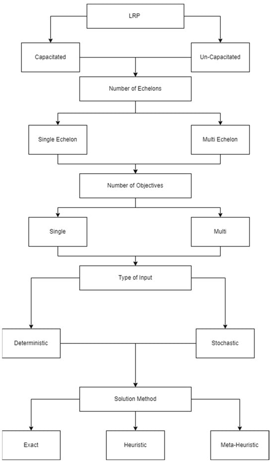
Figure 2.
LRP classification.
2.6.1. Problem Type
Initially, most researchers and scholars focused their efforts on uncapacitated LRP, but since the beginning of the 21st century, the focus has shifted to CLRP. This is the result of CLRPs being more representative of the real-life case [31]. This result was also reciprocated by a study conducted in 2017 by Michael Schneider and Michael Drexl [32] and another study conducted in 2021 by Setyo Tri Windras Mara et al. [33]. After the overall type of problem is defined, the scale of the problem is then introduced.
2.6.2. Number of Echelons
The scale of the problem is introduced by determining how many echelons to tackle. A single echelon, for example, could determine the location of the facility, then determine the routes to take to the suppliers. If the distribution centers are to be added, then the problem shifts from being a single-echelon to being a two-echelon problem. In sense, the two echelons came from the idea of dividing the problem into two: an LRP between the facility and suppliers, and another LRP between the facility and the distribution centers. The same could be said if a relay or a secondary facility is added to the original problem of only the facility and the suppliers. Then, the problem again shifts from being a single-echelon to being a two-echelon problem.
Two-echelon LRPs are very common in the literature, since they are a more realistic presentation of real-life logistics. Yong Wang et al. studied a two-echelon, multi-depot LRP with pickup and delivery. The aim of the study was to minimize the total operation cost and to improve the overall efficiency of the network. The scope of the model constructed was one logistics center serving multiple pick-up depots and distribution depots. This serves as the first echelon, while the second echelon is between the distribution depots, the pick-up depots, and the customer demand nodes [34]. Valeria Soto-Mendoza et al. tackled a collection and delivery open-location problem, which is a classic variant of LRP. The two-echelon model was constructed with one echelon collecting the required raw material from the suppliers, while the second echelon was responsible for delivering the final product produced to the customer nodes [35]. Xi-Dan Tian and Zhi-Hua Hu conducted a study of a two-echelon LRP with fixed relays. The first echelon was concerned with the transportation of the goods from the facility to the chosen relays, while the second echelon was responsible for the distribution of the goods from the relays to the customer nodes [36]. It can be seen from the literature sample presented that the meaning of a two-echelon LRP may differ from one variant of LRP to another. Figure 3a,b show the difference between a single-echelon and two-echelon problem.
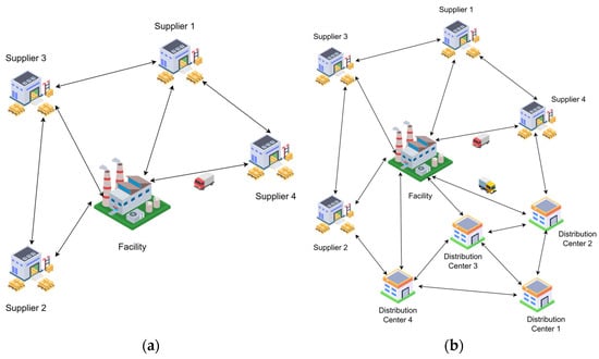
Figure 3.
(a) An example of a single echelon; (b) an example of two echelons.
2.6.3. Number of Objectives
LRPs can be single-objective or multi-objective in nature. Single-objective means that the only aim is to minimize cost. This cost could harbor multiple factors varying from fuel consumption to contracting costs of suppliers or avoiding delay penalties. While multi-objective is next to where the cost is being minimized, there is another objective, such as improving efficiency or waste management. It is worth mentioning that some authors consider the reduction in the cost of multiple objectives as a multi-objective problem.
Abed Zabihian-Bisheh et al. tackled an LRP with the goals of minimizing the costs of location and transportation of harmful waste to certain disposal locations. The model’s aim was to minimize the waste management system cost, the hazards of the facilities, and transportation and carbon emissions from transportation [37]. Jianhui Du et al. constructed a two-echelon, multi-depot joint delivery model to tackle an LRP with the aim of minimizing operational costs and carbon emissions. Another objective targeted by the authors was to achieve maximum customer satisfaction [38]. Yuhe Shi et al. tackled a simultaneous location and routing problem for parcel delivery and recyclable express packaging recycling. The purpose of that study was to reduce operational costs and vehicle working times [39]. The aforementioned literature shows that several of these studies conducted by their respected authors have mentioned clearly that one of the aims of the study was to achieve sustainable behavior, specifically sustainable behavior regarding the environmental pillar.
2.6.4. Type of Input
When discussing the types of input, the type of data served as input to the model is what comes to mind. Two main types of data input are seen to be used with LRP: deterministic and stochastic or fuzzy. The deterministic type of data input is the simplest type to use. The data are given in the form of constant values; this could be transportation times, distances between locations, and even time frames for which delivery and pickup from locations are allowed. For stochastic data which can be called fuzzy, there is uncertainty in the data. This uncertainty could be the demand asked by a customer, uncertainty in travel times between locations, and so forth. This uncertainty is usually modeled using probabilistic or fuzzy equations. Masoud Hajghani et al. approached an LRP taking into consideration the three pillars of sustainability. The model constructed was a two-echelon model with open and closed routing. The uncertainty rose from the amount of constraints applied to the model. To counter such an effect, the authors opted to deploy a probabilistic model to deal with the uncertainty of the data [40]. Alan Osorio-Mora et al. tackled a variant of the classical LRP, the latency LRP. The uncertainty presented in the model is in the travel times between locations. The authors offered additional insight by stating the risk level in the solutions produced [41]. Alireza Eydi and Pardis Shirinbayan tackled a multi-commodity multi-model hierarchical hub location problem with uncertain demand. The uncertainty presented in the model comes from the fuzzy demand of the customer in which the customer demand is uncertain [42]. Another case worth mentioning is the periodic demand case. It is not an uncommon case that customer nodes or suppliers may require multiple visits every period of time, for example, on certain days of the week. In this case, the schedule of each customer or supplier is also required. This type of problem was first introduced by Prodhon in 2008 [43].
Periodic data is not necessarily a data type in sense, but it can be considered as data type since it is given as an input. Normally, no single type of data input is dominant in these problems but rather a mixture of deterministic with stochastic, deterministic with periodic, or stochastic with periodic. Imen Ben Mohamed et al. tackled a two-echelon distribution system with uncertainty. The uncertainty comes from the demand of the customer nodes while also requiring future visits for delivery, hence the periodic segment [44].
2.6.5. Solution Methods and Applications
Three main categories of solutions could be found in the literature: exact, heuristic, and meta-heuristic methods.
Exact method: Ece Arzu Yıldız et al. utilized an exact branch and cut algorithm (B&C) to solve a two-echelon LRP with simultaneous pickup and delivery. In this study, the authors were able to provide optimal solution for up to 50 customers and 10 relays in reasonable computational time. The model was then deployed in a case study of a two-echelon supermarket distribution system in Turkey [45]. Bencomo Domínguez-Martín et al. used another B&C algorithm to solve an LRP with the one-commodity pick-up and delivery traveling salesman problem. The model had the aim of reducing the overall cost of the routes taken and the facilities used. The model was able to solve instances up to 100 nodes [46]. Maria Barbati et al. developed a multi-objective evolutionary technique with the name of NEMO-II-Ch which takes into consideration the preferences of the user. This algorithm was then compared to three other algorithms, which resulted in the model being superior to these models in terms of time [47]. While exact solutions are preferred for accuracy, it has been proven that it takes significant computational time and power to achieve the target required. In addition, with increasing difficulties and complexities of problems introduced, the focus turned to heuristics and meta-heuristics to be used for these types of problems with only a near-optimum solution as a target.
Heuristics and meta-heuristics: Dekun Tan et al. utilized a heuristic artificial bee colony algorithm to solve a two-echelon location-routing problem with pick-up and delivery. The model constructed was a multi-objective model with the aim of reducing the overall cost and carbon emissions as a result of transport. The algorithm was then compared to four other heuristic algorithms on simulated instances and a real-life case. The proposed algorithm outperformed the other heuristic algorithms in a relatively short time [48]. Naman Mahmoudi et al. utilized a meta-heuristic algorithm in order to tackle a single-hub same-day delivery transportation problem. The genetic algorithm’s aim was to minimize the transportation costs in scenarios where demand could be split among nodes. The algorithm was then tested in a case study, showing good performance [49]. Mi Hu et al. addressed a multi-period emergency facility location-routing problem, in which the uncertainties in material demands and transportation time were analyzed using a meta-heuristic algorithm. The algorithm was tested on several instances and applied to the real case study of the Wenchuan earthquake in China. The algorithm performed significantly better when compared with a Gurobi solver in terms of quality solutions and computational time [50]. Behrang Bootaki and Guoqing Zhang utilized another genetic algorithm to solve the LRP. The algorithm tackled three different types of decisions: the facility location, production planning, and routes planning. The genetic algorithm used was a hybrid method mixed with artificial neural networks and called the neural genetic algorithm. The algorithm produced near-optimum results, with a gap of 3% and 99% enhancement in computational time [51].
2.7. Literature Findings and Gap
Several conclusions could be deducted from the previously discussed literature. With the emphasis of scholars on the necessity of implementing social aspects in supply chain decisions, it seems that it is still being ignored or overlooked due to the challenges mentioned earlier. In the LRP context, the social aspect is still not heavily integrated, with the focus mainly being on environmental and economic aspects. This could be deducted from the goals mentioned earlier by each research article discussed. The first highlight was the overall minimization of costs; this serves as the economic pillar. The second highlight is that some articles are taking into consideration their carbon emissions or waste management; this serves as the environmental pillar. The nearest article to remotely discuss the social pillar is the one authored by Masoud Hajghani et al., where the social aspect proposed was an increase in employment rate [40]. This is very relatable, as discussed earlier, where the social aspect is seen as job creation or community development, as highlighted by Kravchenko et al., Padilla-Rivera et al., and Roos Lindgreen et al. [5,6,7]. The second-nearest article which may have contributed to social sustainable behavior was the one authored by Yuhe Shi et al. In this article, the vehicle working times were considered which may or may not indirectly contribute to the human factor of the vehicle, which is the driver [39]. It is important to mention that the majority of the research published by fellow scholars is directed towards big enterprise logistics. In concept, the algorithms proposed will provide solutions for both big enterprise logistics and SME logistics. However, not all solutions could be feasible for SMEs, since big enterprises have the capability of allocating larger funds in comparison to SMEs. As a result, the solutions proposed may not be appealing for implementation by SMEs, further complicating the issue.
3. Methodology
3.1. Research Flow
As the first step, the problem is defined and formulated; this includes explaining the problem clearly and defining the boundaries of the system. The second step is the construction of the model based on the assumptions made and the constraints restricting the model. The third step is model testing; this step is where the model is evaluated to make sure that it is functioning as required. The evaluation is performed in two steps: verification and validation. The fourth step is the experimental work to be implemented in the model. The fifth and final step is the analysis of the results. Each step will first be discussed generally, then extensively explained in a dedicated section. Figure 4 shows the process flow.
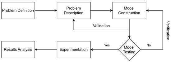
Figure 4.
The proposed methodology.
3.1.1. Problem Definition
In this article, the aim is to integrate the social aspect in the supply chain problem by solving a two-echelon capacitated location-routing problem using meta-heuristics, specifically a genetic algorithm, taking into consideration breaks induced for the driver and the proximity of the facility location to a transportation hub. The proximity of the facility to a transportation hub is already considered a secondary decision in supply chain logistics. Martin Aleksandrov defined the social aspects of vehicle-routing problems, which include aspects such as fairness for drivers and fairness and efficiency for customers [52]. Breaks for vehicle drivers are considered in this study since they are considered as a simple aspect to implement that guarantees some sort of fairness to the driver. These two aspects were specifically chosen since they are feasible solutions to both major enterprises and SMEs. The aim of the model is to minimize the overall cost of operations, making it a single-objective model. Two cases will be discussed: the normal case and the uncertain case.
3.1.2. Problem Description
In the problem description phase, each case is discussed thoroughly. This includes defining the entities within the system, how these entities interact with each other, and the system boundaries. For each case, the scope of the model is defined, the number of entities within the model is set, and the goal which the model aims to achieve is determined.
3.1.3. Model Construction
In this section, the model construction phase is explained thoroughly. First, the assumptions that are related to the problem are defined. Second, the type of input that will be provided is clearly stated. The third step is providing the mathematical notation related to the problem. The fourth step is defining the constraints restricting the problem solutions. The fifth step is defining the objective of the model mathematically. The sixth and final step is the implementation of the algorithm for solving such a problem. The previously discussed steps will be duplicated for both cases, the normal and uncertain cases. This is excluded in the selection of algorithm section since both cases share the same step; hence, it will only be discussed once. Figure 5 shows how the model will be constructed.

Figure 5.
Model construction phase.
3.1.4. Model Testing
In the model testing phase, two steps are performed to make sure the model works as intended: verification and validation. Verification is performed either by static or dynamic testing. In this case, static testing is used where each element in the model is observed by a peer to make sure it behaves as it was first made in the model construction phase. This is followed by corrective action if any element is found not as behaving as intended. Validation, on the other hand, is making sure that the model complies with the initial problem formulated. This could be performed by using a benchmark problem where the mathematical answer is already known [53]. This step is shared between both cases since the base model for both cases is the same.
3.1.5. Experimentation and Validation
In the experimentation phase, a set of experiments is developed in order to determine certain aspects. In LRPs, the accuracy of the mathematical result of the model is usually discussed. This is performed by comparing the result produced to the exact answer to the problem or the ground truth. This accuracy can be interpreted in two different values: the mean value of the test runs made on the model and the root mean square error (RMSE). Both values are discussed among other aspects that will be further investigated for each case.
In the following sections, the research flow discussed will be duplicated for each case, further detailing the various steps already highlighted.
4. Case Study
4.1. Research Flow Application
In this section, each case study is tackled based on the methodology explained in Section 3. Some parts of the methodology will be shared between the two cases since the steps are identical.
4.1.1. Problem Description: Normal Case
The normal case was discussed early on in the selection of the main facility, the suppliers and distribution centers to contract with, and the routes to be taken. The locations of five facility locations are identified to be selected from, and a shortlist of twenty suppliers and distribution centers to choose from, with ten for each side. Each facility is assigned a purchasing fee. Each supplier and distribution center are also assigned a contracting fee and a capacity. The capacity for the suppliers is the amount of supplies that could be taken from this supplier while the capacity for the distribution centers is the number of products that could be distributed through that specific center.
Two versions of the normal case are tackled: the first case is where it is requested to contract three different suppliers and three different distribution centers, and the second case is where the number is increased to four from each type. This was achieved as a level of flexibility for the model as an attempt to tackle multiple scenarios. Two vehicles are assigned to the problem with each vehicle handling one of the echelons. The first echelon is between the suppliers and the main facility location and the second echelon is between the main facility and the distribution centers. The number of vehicles was chosen based on the assumption of the worst-case scenario which is that supplies are required to be brought in to the facility and products are to be distributed from the facility at the same time. Six transportation hubs have been added so that the distance from the facility is taken into consideration. Figure 6 shows the scope of the model.
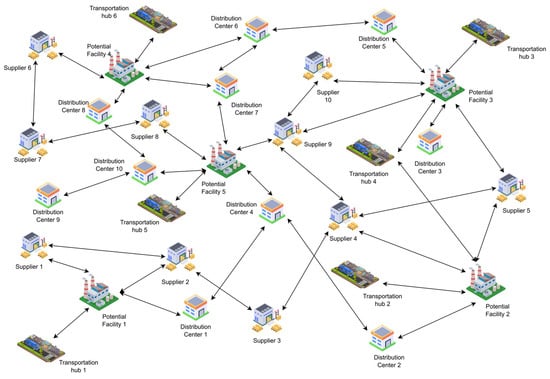
Figure 6.
A conceptual model of a normal case.
4.1.2. Model Construction: Normal Case
Definition of Model Assumptions
In this section, several assumptions are made that will be applied to the model. In addition to the assumptions previously defined by authors in their respected models in the literature, several assumptions that are specific to this model are also added.
- Assumptions that are used by other authors in the literature:
- Each vehicle can, at most, be at one location at any time.
- The vehicles must start and end at the facility location.
- Each of the two vehicles is assigned to one type of destination (one for suppliers and the other for distribution centers).
- Temporary visits are made to the facility in case the vehicle assigned is fully capacitated for suppliers or empty in case of distribution centers.
- The capacity of both vehicles is equal.
- The cost of leasing/renting both vehicles is equal.
- The number of suppliers required is equal to the number of distribution centers needed.
- Assumptions that are specific to this research article:
- The break time duration for each driver.
- The break rate, in USD, per break.
- The compensation fee for proximity to a transportation hub.
- Number of employees in facility.
Definition of Model Input
- The following information is provided in the model:
- The locations of each possible facility for purchasing, the suppliers, and distribution centers for contracting are given.
- The capacity of each vehicle is given.
- The capacity of each supplier and distribution center is given.
- The distances between each location and the other are given in Euclidean distances.
- The cost of each facility location, each supplier, and distribution center available for contracting are given.
- The cost of fuel liter per kilometer is given.
- The cost of carbon emissions per kilometer is given.
- The leasing/renting cost for each vehicle is given.
- The tank capacity of both vehicles is given.
Creation of Mathematical Notation
In this section, the mathematical notation used is shown in Table 1. showing each symbol and its meaning. These symbols will then be used to construct the mathematical model by expressing the constraints afflicted on the model, as well as the model objective.

Table 1.
Mathematical notations and their explanation.
Definition of Model Constraints
In this section, the constraints that will be applied for the model are explained with their mathematical notation.
- No vehicle can be at multiple locations at the same time:
- The trucks should start and finish at the same point:
- A total of three or four suppliers are required (in case of both versions of the model):
- A total of three or four distribution centers are required (in case of both versions of the model):
- The capacity of both vehicles at any time cannot exceed the value of 30:
Definition of Model Objective
The main objective is to minimize the overall cost of operations. The objective function is divided into three sections: each section is related to one of the pillars of sustainability, environmental, economic, and social. For the environmental section, the distances covered by the vehicles reaching the different locations is translated into cost by multiplying of the distances by the cost of carbon emissions per kilometer given as an estimate. For the economic section, it includes the cost of purchasing the facility location, the leasing or rental of both vehicles, the contracting fees for both the suppliers and distribution centers, and the fuel consumption of both vehicles. For the social aspect, two aspects were considered: the breaks taken by both drivers during their transportation and the proximity of the main facility to a near transportation hub. These aspects are introduced as penalties where the number of breaks that are induced are counted and the driver is compensated with a monetary value, and the proximity to the hub is a compensation fee offered to the employees based on the distance to the transportation hub.
4.1.3. Problem Description: Uncertain Case
The second case is where uncertainty in the market demand occurs, causing an increase in the production that cannot be fulfilled using a single facility. The main facility chosen from the first model is expected to run at 80% of its production capacity. If the demand increases by an extra 10%, the assumption is made that it can be handled by increasing the number of shifts. Any further demand cannot be occupied by the main facility. As a result, a secondary facility is required to work next to the main facility to support the production. The secondary facility will also act as a relay to convey the delivered goods to the requested destinations. Eight possible secondary facilities are added to the model. Each secondary facility is assigned a purchasing cost and a facility size, four small sized and four medium-sized. Depending on the severity of the uncertainty of demand, the size of the secondary facility is chosen accordingly.
Two uncertainty states are identified. The first state is where the uncertainty in demand may increase from 10% of the market demand until 40%. In this state, a small-sized secondary facility will be selected. The second uncertainty state is where the uncertainty in demand may vary from 40% to 70%. In this case, a medium-sized facility will be selected. No case further than 70% was tackled due to the unlikelihood of the case and the incapability of an SME to handle such load. In a case where uncertainty is between 10% and 40%, four suppliers and four distribution centers will be selected from the available list for contracting. If the demand is between 40% and 70%, the number of suppliers and distribution centers are increased to five. As implemented for the first model, this was achieved as a level of flexibility to the model to accommodate different sizes. The two vehicles assigned in the first model will be replaced with another two vehicles of bigger capacity and a penalty for abandoning the lease of the older vehicles will be implemented as a fixed cost. The two vehicles will also serve both the main and secondary facilities. Figure 7 shows the scope of the model.
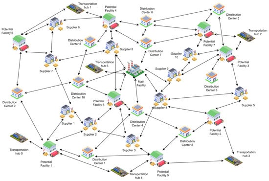
Figure 7.
A conceptual model of the uncertain case.
4.1.4. Model Construction: Uncertain Case
Definition of Model Assumptions
In addition to the assumptions made earlier in the normal case model, some assumptions are modified:
- Temporary visits are made to the main facility and secondary facilities in case the vehicle assigned is fully capacitated for suppliers or empty in case of distribution centers;
- The tank capacity of the new vehicles is the same as the old ones;
- The number of employees in the main facility is equal to the number of employees in the secondary facility;
- The compensation fee given to the employees in the main facility is the same as the one given to the employees in the secondary facility.
Definition of Model Input
As extra information added to the information mentioned in Section 4.1.2.
- The locations of the secondary facilities to select from are given;
- The purchasing value for each facility is given;
- The fixed cost inflicted as penalties for abandoning the old vehicles’ leases is given;
- The new leasing/renting value of the new vehicles is given.
Creation of Mathematical Notation
In addition to the previously mentioned mathematical notations, several new ones were added to accommodate for the uncertain case model. Table 2 shows the addition to the original mathematical notation.
Table 2.
Mathematical notation and their explanation.
Definition of Model Constraints
In this section, the new set of constraints that are applied to the uncertain case model are explained with their mathematical notation.
- No vehicle can be at multiple locations at the same time:
- The trucks should start and finish at the same point:
- A total of four or five suppliers are required (in case of both versions of the model):
- A total of four or five distribution centers are required (in case of both versions of the model):
- The capacity of both vehicles at any time cannot exceed the value of 40:
Definition of Model Objective
Several additions were added to the original objective function to accommodate the changes to the model. These additions are the cost of purchasing the secondary facility, the penalty of abandonment of the old vehicles, and the lease/rent of the new vehicles. The compensation fee given to employees in the secondary facility for distance from the nearest transportation hub is also taken into consideration.
4.2. Selection of Algorithm
Meta-heuristic methods were selected as the solving technique in this problem for multiple reasons. The first one is that the more complex the problems become, the more difficult they are to be solved using exact methods. The second reason is the computational power and time required to solve such problems. Meta-heuristics have proven their capability of handling such problems at much lower computational times and with minimal power required in comparison to the exact methods. Evolutionary algorithms have been used extensively in the literature, as demonstrated by Dekun Tan et al., Naman Mahmoudi et al., and Qing-Mi Hu et al. [48,49,50]. For this problem, a genetic algorithm will be used to solve both cases, the normal and uncertain cases, previously discussed. The genetic algorithm was chosen since it has proven its effectiveness with such problems, as shown by Naman Mahmoudi et al. [49]. Its ability to be used as a hybrid technique and producing near-optimum results, as shown by Behrang Bootaki and Guoqing Zhang, is also a strong point [51]. The DEAP library has been utilized in this research for its flexibility and the wide variety of operators that can be used [54]. For the genetic algorithm, there are several aspects to consider. First, the initial population is generated fitting the initial assumptions and constraints made to both case models. The parents that will be used for crossover will be selected based on certain selection techniques. The crossover and mutation agents are then selected. The algorithm is then executed multiple times until the termination criteria is reached. Figure 8 shows how the genetic algorithm operates.

Figure 8.
The steps of the selection method.
4.2.1. Initial Population Generation
The initial population is the population of feasible solutions that can be considered. This means that these solutions abide by the model assumptions and respect the constraints inflicted on the model. The feasible solutions in question are the routes that can be taken by the vehicles, showing the stops that the vehicles will make. The initial population for the normal case differs from the uncertain case due to the different requirements of the solution. Both cases’ initial populations will be discussed in detail.
- Normal Case: Initial Population;
The solution is presented in the form of a chromosome; the chromosome represents the route that will be taken by both vehicles to reach their destination. The chromosome is divided into genes or bits, with each bit showing where the vehicle had its stop whether at a main facility or at a supplier or distribution center. To accommodate both model sizes of the normal case, two different functions were created. The first function populated an 11-bit-sized solution and the second function populated a 13-bit-sized solution. Since there are two vehicles, each servicing one of the echelons, the chromosome is divided into two. The first half of the chromosome shows the routes taken by vehicle M between the main facility and the suppliers, while the second half of the chromosome shows the route of vehicle K between the main facility and the distribution centers. Since there are five main facilities to consider, five subsections of the initial population function were created to produce a solution for each main facility. Despite the fact that this could have been made within the same population generation function, it was decided that the choice should be given to the user of the algorithm to decide which of the five main facilities which to use.
The numbering of the facilities works as follows: the facilities are numbered from one to five, the suppliers are numbered from six to fifteen, and the distribution centers are numbered from sixteen to twenty-five. The initial chromosome only shows the numbering of the main facility in multiple bits, indicating that this is the time allowed for one of the vehicles to stop at the main facility. The remainder of the bits is left assigned a number zero. The function then starts the creation of the initial routes by randomly selecting values in the bits allocated for the suppliers and distribution centers. After the randomization is completed, the function then checks that the route would respect the capacity constraint of the vehicle, which should not pass the threshold of thirty. If a part of the chromosome fails the criteria, the function keeps on generating random numbers until the capacity constraint is respected. If the chromosome created is already a duplicate of a pre-existing chromosome, the chromosome is eliminated and another chromosome is generated. This process continues until the number of initial solutions required has been reached. Figure 9 shows an example of a chromosome for main facility number 1 with the suppliers and distribution centers selected and the route shown.

Figure 9.
Example of chromosome for normal case.
- Uncertain Case: Initial Population.
The uncertain case continues after the normal case; the main facility had been selected earlier, with the focus on the secondary facility. The chromosome of the uncertain case as the normal case is divided into two segments, with each segment serving one of the echelons. The chromosome size in the uncertain case differs from the normal case depending on the level of uncertainty. The chromosome for the minor case of an uncertain increase in demand ranging from 10% to 40% is a 16-bit-sized chromosome, while the major case chromosome is an 18-bit-sized one. Unlike the normal case, the function for the initial population generates all feasible solutions within the same population, taking into consideration the different secondary facilities. In this case, the choice was not to subdivide since the risk of choosing a secondary location was deemed lower in comparison to choosing the location of the main facility.
The initial chromosome is given with the facility already implemented in certain bits, knowing that at these times the vehicle shall return to the main facility location. For the bits assigned to the suppliers, distribution centers, and secondary facility, they are assigned the value of zero. The same numbering of the suppliers and distribution centers is used in the uncertain case. The numbering of the secondary facilities is given, from thirty to thirty-seven. From thirty to thirty-three is for secondary facilities of small size, and thirty-four to thirty-seven is assigned to secondary facilities of medium size. The function then randomizes values for each bit that is assigned a zero. The next step is checking the capacity constraint. If the constraint is not respected, the function keeps on randomizing numbers until the capacity constraint is applied. The function then checks the chromosome for duplicity. If the chromosome is duplicated, it will be eliminated and another chromosome will be generated. The function continues on generating chromosomes until the required number is reached. Figure 10 shows how the chromosome is changed from its initial form to the final feasible solution form.
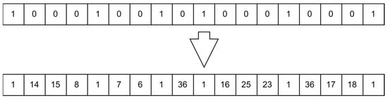
Figure 10.
Example of chromosome for uncertain case.
4.2.2. Parents Selection
The parents that will be chosen for breeding can be chosen using different parent selection methods. Many techniques are found in the literature on how to select parents. For this problem, three different selection techniques were chosen: the tournament selection technique, the stochastic universal sampling (SUS) selection technique, and the elitism selection technique. The three techniques were chosen for different reasons. Tournament has proven itself to be researchers’ favorite technique due to its versatility. On the other hand, SUS has proven itself in minimization problems. Elitism, which is considered to be the newest of the techniques in terms of age, has also proven its worth in enhancing results. Each technique will be discussed in detail.
- Tournament Selection
Tournament selection is a random selection technique based on the fitness value of the solution. This means that for each solution provided in the initial population, a fitness value f is assigned based on the quality of the solution. In this case, the value comes from the model of the objective. Equations (11) and (25) are used to assign the fitness value for each solution. The number of parents is set by the user, and this number is used to randomly select the parents from the population. The tournament size k is set to initially select the number of individuals that one parent will be chosen from. These individuals are then evaluated based on their fitness value, and the best fitness value parent is selected. The best fitness value in this case will be the individual with the lowest fitness score since the fitness score is cost and the aim is to minimize the cost. This process is then repeated a number of times, equal to the number of parents needed [55]. Figure 11 shows how the tournament process is carried out.
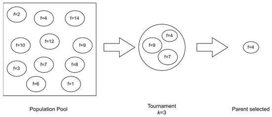
Figure 11.
Example on tournament selection.
- 2.
- Stochastic Universal Sampling (SUS) Selection
The SUS technique is a subset of the original roulette technique. The original roulette technique first calculates the total fitness value of the entire population. The selection probability is then set as value for every chromosome, and the cumulative probability is calculated for every chromosome. A random value r is generated between [0,1], and if , then the chromosome is selected. These values are then set in a pie wheel with one pin to stop the wheel. The sizes of the pie on the wheel differs depending on the fitness value of the solutions. The problem with such a technique is that it is biased towards the stronger chromosomes, limiting the variety of the solutions that could possibly be better [55]. As an enhancement to this technique, SUS is used. The difference between the two techniques is that the total number of parents are selected at the same time in the SUS technique. This is achieved by using an outer wheel on the pie with pins that are equidistant from each other. The number of pins is equal to the number of parents required. This guarantees that there is less bias in the selection process. Figure 12 shows the difference between the standard roulette and the SUS technique.
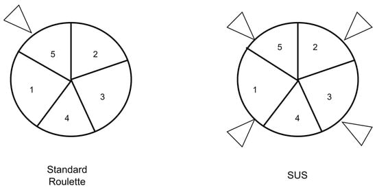
Figure 12.
Difference between roulette and stochastic universal sampling.
- 3.
- Elitism Selection
Elitism could be used as a hybrid parent selection technique or as a standalone technique. This means that it could be mixed with another type, such as tournament selection, or it could be used as a standalone process. Elitism, as a technique, ensures that the best individuals continue to the next stage untouched. For the hybrid case, the parents are selected using the normal method. In the case of tournament selection, tournament is first applied, and then the parents are used for creation of offspring. In this case, the best of the parents is withheld from the population and added to the new population that will be used later on. This number could differ; the number of elites can be controlled so that not only one parent is withheld, but multiple ones. The criteria for withholding will be the fitness value of each parent. In the standalone case, the parents are selected from the initial population using their fitness value. This means that the entire population is evaluated, and if the number of elites, for example, is five, the top five individuals in the population are chosen as the parents. After the breeding process is completed, these parents are withheld so that they are not lost with the older population and are transferred to the new initial population. This ensures that the strongest individuals survive across the generations [55].
4.2.3. Crossover Agent Selection
In reality, crossover mimics biological combination. A portion of the chromosome is swapped with another to produce an offspring. The same concept applies to the genetic algorithm. Two solutions are partially swapped to produce a new solution. The only solutions considered are the parents which were previously selected using the parent selection techniques. Three crossover agents are considered for utilization: one-point crossover, two-point crossover, and uniform crossover. Each agent will be explained in detail.
- One-Point Crossover
In one-point crossover, a random point is selected in the chromosome length of one parent, and that same point is selected in the chromosome of the other parent. The chromosome is then divided at that point and swapped between both parents to create two new offspring. The first half of the first parent is swapped with the second half of the second parent, and the first half of the second parent is swapped with the second half of the first parent [55]. Figure 13 shows how one-point crossover works.
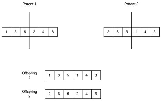
Figure 13.
One-point crossover.
- 2.
- Two-Point Crossover
Similarly to how one-point crossover works, two random points are selected for the parents and the chromosome bits selected are swapped between the two parents creating two new offspring [55]. Figure 14 shows how two-point crossover works.

Figure 14.
Two-point crossover.
- 3.
- Uniform Crossover.
Uniform crossover works as a random gene selector operator. This means that bit by bit, the crossover passes over the chromosome. Each parent is assigned heads or tails as a coin, a random toss is performed, and the selected parent occupies this part of the chromosome. Similarly, the second offspring is the exact inverse of the first offspring. Uniform crossover does not need to pass over the entire chromosome. Only a segment of the chromosome could be used for the offspring creation [55]. Figure 15 shows how uniform crossover operates.

Figure 15.
Uniform crossover.
4.2.4. Mutation Agent Selection
While there are multiple operators that can be used in the literature, none fit the description of what is required. A special function was created to perform the mutation process. Mutation occurs in the offsprings that were created from the crossover process. Based on the percentage of mutation, multiple bits could be mutated to give variety to the solutions produced, hence emphasizing exploration. The created function checks certain aspects before mutation. If the bit is assigned a value regarding a main facility, the bit remains untouched. The only bits that are allowed to mutate are the ones responsible for the suppliers and distribution centers. Once the bit is mutated, a check is made to see whether there is a duplicated number; this means that there are two bits having the same supplier or two bits that have the same distribution center. In case there is duplication, the mutation is repeated until no duplication occurs. The second check the function employs is the capacity constraint check. The function makes sure that the capacity constraint is respected. If not, the mutation reoccurs until the chromosome becomes feasible. Figure 16 shows how the mutation process occurs.
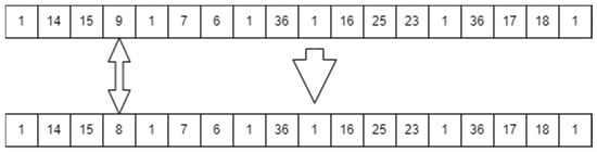
Figure 16.
Example of a mutation agent.
4.2.5. Algorithm Execution
In this section, the method of execution of the algorithm will be discussed in detail. Each case will be tackled in a separate section. While the algorithm for both cases is the same, the method of execution is not similar; hence, the sections will be separated.
- Normal Case
Since the selection of the main facility is an important decision to make, the algorithm is divided into five subsections. Each section shows the feasible solutions regarding only one facility. This means that there are five different genetic algorithms that run in parallel. The algorithm first uses the initial population function in order to create the feasible solutions. The parent selection process then starts until the number of parents set by the user is reached. The three previously defined techniques are used in parallel to determine the parents. The crossover and the mutation processes start to create the offspring. These offspring, for extra security, pass through a validity check to make sure that they respect the model’s assumptions and constraints. Afterwards, the offspring replace some individuals from the population. The individuals replaced are usually the ones with the lowest fitness score; hence, they will no longer be considered. The algorithm keeps on executing until the termination criteria is reached. Five different results, one for each location, are shown. Figure 17 shows how the algorithm is executed.
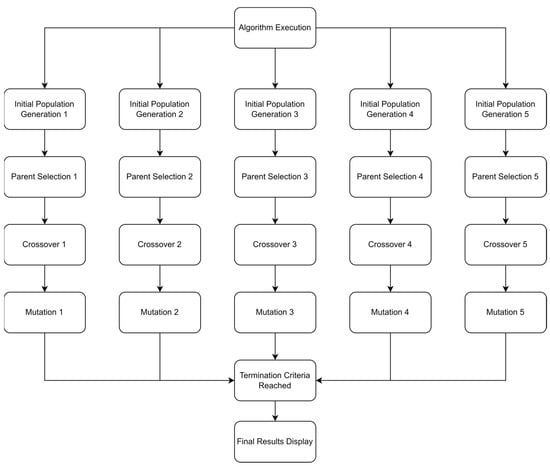
Figure 17.
Algorithm execution: normal case.
- 2.
- Uncertain Case.
For the uncertain case, the algorithm execution sequence is the same. However, the process is not duplicated for the secondary facilities. This means that for each stage, all secondary locations are considered at once. The initial population stage includes only one function that generates all possible solutions for the different secondary facilities. The parent selection process is then initiated using the different techniques. The crossover and mutation agents are utilized, and once the termination criteria is reached, the algorithm displays a single final result. Figure 18 shows how the algorithm is executed.

Figure 18.
Algorithm execution: uncertain case.
4.2.6. Termination Criteria
The termination criteria are user-dependent; the user can set a certain number of generations which when reached, the algorithm terminates its execution, and the solution reached is displayed with its fitness score. The other termination criterion that could be set is time. After the algorithm runs for a certain amount of time, it terminates, showing the solution reached and its fitness score. For the normal and uncertain cases, the number of generations is set as the termination criteria, and the time for each run is recorded.
4.2.7. Model Testing Steps
Model testing is performed by verification and validation. Verification is the first step, since this ensures that the model follows the assumptions and constraints made by the user. Validation follows afterwards, affirming that the mathematical values produced are correct.
- Verification
Intuitively, verification is performed by peers to make sure that the model is constructed correctly. In this case, this is performed by making sure that the solution produced follows a certain sequence. The chromosome design is key to this step, since it shows the sequence of locations that the vehicle passes by. By checking the logic of the sequence, verification is made. The checks that were considered for verification are as follows:
- The chromosome is divided into two sections: the first half is for the first echelon and the second half is for the second echelon. This is performed by checking the numbering assigned for each bit, since the suppliers and distribution centers have different numberings.
- No duplication of bits; this means that the numbering of the bits that are assigned to the facilities are different from the other bits.
- The size of the chromosome is the same after crossover and mutation. This ensures that the length of the chromosome is the same after any step.
- The capacity constraint is respected; this is performed by manually calculating the capacities of the bits to make sure that they uphold the capacity constraint.
- 2.
- Validation
Validation makes sure that the numerical values produced from the model are correct. This means that the fitness score of the chromosome produced is calculated correctly. Validation through literature is performed using a benchmark problem, a problem where its fitness score is known. In this article, no benchmark was used, since the problem is of the authors’ design. This was made to induce stochastic noise into the problem, since most benchmark problems do not consider noise. Stochastic noise in this case is induced by designing the problem with multiple solutions which have the same fitness score. For example, the sequence [1, 7, 8, 1, 6, 1, 17, 18, 1, 23, 1] can have the same fitness score as [1, 8, 7, 1, 6, 1, 18, 17, 1, 24, 1].
Validation was performed in two steps. First, a small instance was constructed so that the fitness score could be checked. Out of a pool of four suppliers and four distribution centers, only two of each type are required. A problem of that scale can have a total of sixteen solutions. This minor model was validated by using a linear programming model (LPM), which is an exact model. The sixteen solutions were also solved manually to make sure that the LPM was functioning correctly. Comparison with the algorithm was made to make sure that it complied with the manual calculations and the LPM. Only a single parent selection method out of the three was used for validation. The second step was constructing two LPMs, each accommodating one of the cases, the normal and the uncertain to validate each model. The exact fitness value for each model was then reached and validated against the problem design. Figure 19 shows the steps performed for validation.
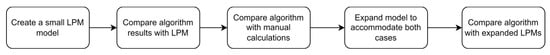
Figure 19.
Steps taken for validation.
5. Experimentation
As previously mentioned, the criteria for evaluating the performance of meta-heuristic models is the accuracy of the model. This accuracy can be interpreted in two numerical values which are the mean value of the test runs and the RMSE. In this study, these values will be used as the criteria for the model performance. It was seen in the literature that the major focus of discussion is usually on the crossover and mutation agents, with minimum to no focus on other aspects. Some of the aspects that were found to be given minimal attention are as follows: the specific initial population size to start the iterations with, the parent selection technique to be used, the specific number of generations to use as termination criteria, and the percentage distribution of parents among the crossover and mutation. While the mutation and crossover agents are very important to discuss, having an idea beforehand on which values for the other aspects to use may reduce the computational time and power is needed. Hence, the aim of this study, for both the normal and uncertain cases, is to shed light on which values to start the experimental runs with that would ensure high success rates. These values cannot be generalized to any problem that is solved using metaheuristic methods, but they can be generalized to an LRP of this magnitude. For each case, the mean and RMSE are evaluated in different perspectives. These perspectives will be discussed in detail for each case.
5.1. Normal Case
For the normal case, the problem is of medium size, with the algorithm proving successful in finding the minimal fitness score and the correct route. Hence, a series of runs is designed to determine the number of instances where the algorithm was successful in achieving the score. The series of trials was only tested on a single location for the main facility since the algorithm runs five different sub-algorithms in parallel. The main umbrella for experimentation would be to determine which parent selection method is the best for the model. Four different parent selection methods were chosen for the testing process: tournament, SUS, tournament hybrid with elitism, and SUS hybrid with elitism. These parent selection methods were chosen for multiple reasons. Tournament was chosen because of its lower sensitivity to stochastic noise. SUS was chosen due to its ability to solve minimization problems. Their mixing with elitism was performed to see whether the performance of the model would improve with its addition. The programming language used for the model was the Python programming language. The platform used for computation was Google Collab, which offers the computational power of an Intel Xeon CPU with 13 GB Ram.
5.1.1. Parameters Setting and Calibration
Under the umbrella of the parent selection methods, the size of the initial population of solutions PS was also tested. Three main levels were designed for experimentation: the first level is at 300, the second level is at 600; and the third level is at 1000. These levels were specifically chosen to test different initial populations, starting from a relatively small value, which is 300, until reaching a medium-sized value, which is 1000 . For the termination criteria, percentages of the initial population were chosen to ensure fairness of the tests across the different populations. Three levels were also set to decide when to terminate the algorithm: 75%, 100%, and 125% . For example, if the initial population size is 1000, the three levels for testing would be 750, 1000, and 1250 generations . The previously mentioned levels for the parent selection methods, the initial population size, and the number of generations at which to terminate the algorithm are the main experimentation levels to consider.
Beneath these levels, a series of trials was set to fine-tune the other variables affecting the model. These variables are the type of crossover to use and the percentage between the crossover and mutation. For the crossover, three types are used: one-point, two-point, and uniform. For the percentages of crossover and mutation, three levels were also set: 90% crossover–10% mutation, 80% crossover–20% mutation, and 70% crossover–30% mutation , . For example, for the 90–10% percentage, this means that out of 10 parents selected, 9 will be used for crossover, while only one will be mutated. For the variables, such as the number of parents, number of elites in case of hybrid parent selection methods, and probability of mutation, these values were kept constant across the trials. Table 3 shows the values used for the constant variables.
Table 3.
Values used for constants.
5.1.2. Experimental Runs
Combinations of the crossover type and percentages were made creating a series of nine trials. These trials are shown in Table 4. Ten iterations were made for each trial, and the number of instances where the global minimum was reached was recorded. This means that, for each parent selection method, a total of 810 instances were recorded for a total of 3240 instances across all parent selection methods. Figure 20 shows the experimental results of the normal case.
Table 4.
Combination of variables.

Figure 20.
Experimentation: normal case.
5.2. Uncertain Case
For the uncertain case, the scale of the problem has grown, turning it from a medium-sized problem to a large-sized one. Hence, the algorithm would not frequently reach the global minimum. In that case, the nearest value to the global minimum is the criteria. The experimentation phase for the uncertain case is divided into multiple sections. The same as the normal case, the programming language used was the Python programming language, and the platform used for computation was Google Collab, which offers the computational power of an Intel Xeon CPU with 13 GB Ram.
5.2.1. Parameters Setting and Calibration: First Experiment
The first section tests which parent selection method would get the nearest to the global minimum. The same four parent selection methods used in the normal case were used in the uncertain case. For the initial population size, an extra level was added, which is 3000, to accommodate for the size of the model . The same levels for the termination criteria were set, and the same nine trials were tested. The same constant variables shown in Table 3 remained the same for the uncertain case. Figure 21 shows the steps for the experimentation phase of the first section.
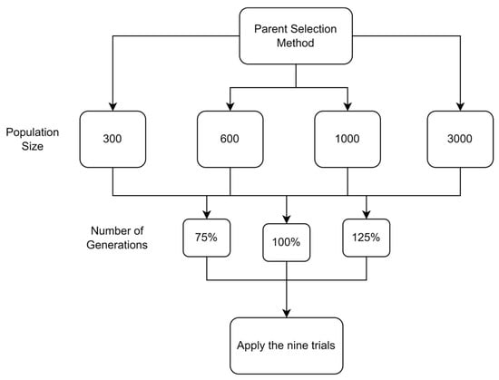
Figure 21.
Steps for first experimentation phase for uncertain case.
- Experimental Runs: First Experiment:
The same as for the normal case, the number of iterations for each trial is also set to ten and an average of the ten iterations is recorded. In the parent selection method, 1080 instances were recorded for a total of 4320 instances for all four parent selection methods. The number of blanks was also collected for statistics. A blank means that the algorithm failed to achieve any result, resulting in a straight horizontal line when plotting the fitness values against the number of generations. The blanks were collected since they give an indication of the stability of the model.
- Performance Metrics: First Experiment:
The instances recorded were evaluated based on the average fitness value produced in each trial. The best scoring trial is then recorded and used for the plotting of the line charts, showing the data trend for the statistical analysis performed on the data.
5.2.2. Parameters Setting and Calibration: Second Experiment
The second section builds on the first section in terms of results improvement. This was made by filtering the trials to find which trial scored the best result in the 125% number of generations. This trial would then be tested at 200% and 300% generations . This was performed as an attempt to determine whether smaller populations would perform better if given a higher number of generations. The parent selection methods would also be filtered depending on the first section. Hence, it is also a comparison between standalone parent selection methods and hybrid ones. Figure 22 shows the steps of the second section.

Figure 22.
Steps for second experimentation phase for uncertain case.
- Experimental Runs: Second Experiment:
Once the best performing trial has been identified, the number of generations is increased to 200% and 300% and ten iterations per trial are run. This produced 320 instances for all parent selection methods. The mean of the iterations is then recorded, and the average time is also recorded per trial.
- Performance Metrics: Second Experiment:
The instances recorded were evaluated based on the average fitness value produced per trial. These averages were then used for data plotting.
5.2.3. Parameters Setting and Calibration: Third Experiment
The final section tests the effect of the number of elites on the model. Four levels were added, which are 3, 5, 8, and 10 elites . After the trials from the first section are recorded, an average performing trial is taken as reference and the number of elites is changed. This was made so that if any improvement is made, it would be noticeable. The fitness score and RMSE were recorded for each trial. For each section, a flow chart showing the steps is constructed. Figure 23 shows the steps of the third section.
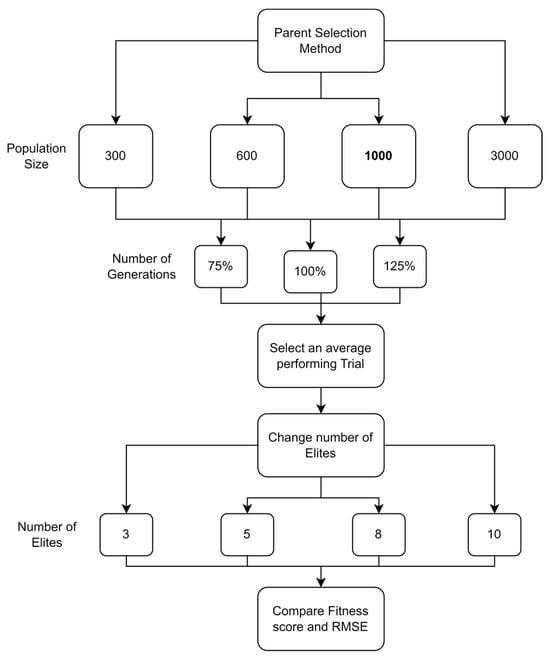
Figure 23.
Steps for third experimentation phase for uncertain case.
- Experimental Runs: Third Experiment:
The number of iterations for each trial is set to ten and an average of the ten iterations is recorded. For each parent selection method, 480 instances were recorded for a total of 960 instances for both parent selection methods. The RMSE for each trial and the average time taken for each trial to be completed were calculated.
- Performance Metrics: Third Experiment:
The instances recorded were evaluated based on the average fitness value produced for each trial. The criteria for evaluating the performance in that case would be both the mean value of the ten iterations for each trial and the RMSE calculated. These variables would then be plotted in line charts to test whether there is an effect of changing the number of elites.
6. Results and Discussion
For the results section, the results of each case are discussed separately. For each parent selection method, they are denoted to differentiate between each one. SUS stands for the combination of SUS with elitism. SUS W stands for using only SUS with no combination. TOURN stands for tournament in combination with elitism. TOURN W stands for tournament with no combination. This presentation is used for both the normal case and the uncertain case. The results shown for each case can differ since multiple runs of the same experimentation phase may show a difference related to the random nature of the genetic algorithm. However, it is believed that very near values will be achieved.
6.1. Normal Case Results
For the normal case, the maximum number of instances that a single parent selection technique can achieve across all levels and trials are 810 instances. SUS W recorded the highest number of instances that is 719 instances. This result was followed by SUS, with 696 instances recorded. TOURN and TOURN W recorded the lowest results, with 552 instances for TOURN and 536 instances for TOURN W. This shows that for a model of medium size, SUS as a parent selection technique is more suitable. It is also evident that the stochastic noise induced had no effect on SUS and tournament as parent selection techniques. Figure 24 shows the number of instances recorded per parent selection method. Elitism had a positive effect on tournament as a parent selection method since the number of instances increased by almost 3%. For SUS, elitism had a negative effect on the number of instances with a decrease of 3%.
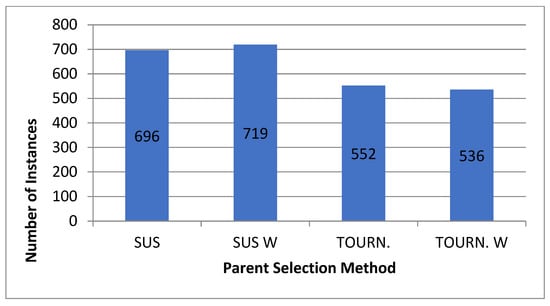
Figure 24.
Number of instances recorded in the parent selection method.
When further investigating the data, the contribution of each trial and the contribution of each population size to the number of instances were explored. For the contribution of trials for SUS W and SUS, no trial was found to be dominant with respect to the number of instances. The difference between each trial and the other is fairly insignificant, with differences of no more than 2%. This shows that the combination of the crossover technique and the percentages between crossover and mutation had no significant effect on the number of instances. This is shown in Figure 25 and Figure 26. For TOURN W and TOURN, the effect was slightly more significant than SUS and SUS W, with a difference ranging between 3 and 3.5%. While the values are a bit more than SUS and SUS W, it is still considered an insignificant effect made by the combination of crossover methods and the percentages of crossover and mutation. Figure 27 and Figure 28 show the effect of the trials on the number of instances regarding TOURN and TOURN W.

Figure 25.
Trial contribution in instances: SUS W.
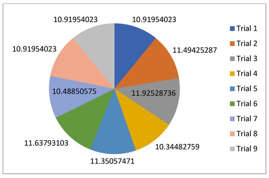
Figure 26.
Trial contribution in instances: SUS.

Figure 27.
Trial contribution in instances: TOURN W.
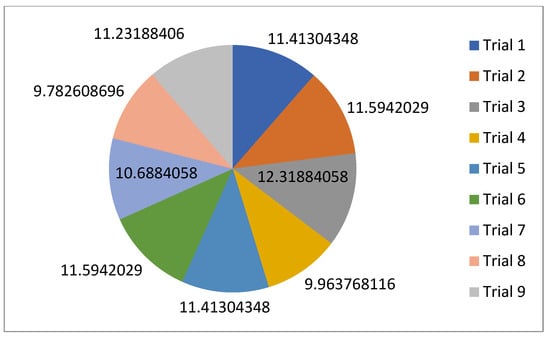
Figure 28.
Trial contribution in instances: TOURN.
For the contribution of the population and the number of generations, the effect varies slightly more than in between trials. For SUS and SUS W, the effect varies slightly more than the effect of the trials. Across a single population size, the change in the effect is less than 1% across the same population size, with the best performing population being the bigger size of 1000. Across all population sizes, the difference in the effect is relatively insignificant, with an increase of 4%. Hence, it can be deduced that it is preferable to use a bigger population size with any number of generations within the levels set for more instances. Figure 29 and Figure 30 show the effect of the population size and number of generations on the number of instances. For TOURN and TOURN W, the effect across population size is significant. Across the same population size, the effect of the generations is relatively insignificant, with an increase of 2%. Yet when the effect across all populations is investigated, it is found that there is a major increase in the number of instances, which rise up to 10%. In comparison to SUS and SUS W, a population size of 1000 was the best performing population size; however, it scored lower values than the ones achieved by SUS and SUS W. Figure 31 and Figure 32 show the effect of the population size and number of generations on the number of instances. The only difference here is the computational time scored. For tournament, the computational time is around 46 s per iteration, while SUS scored a computational time of 51 s per iteration.
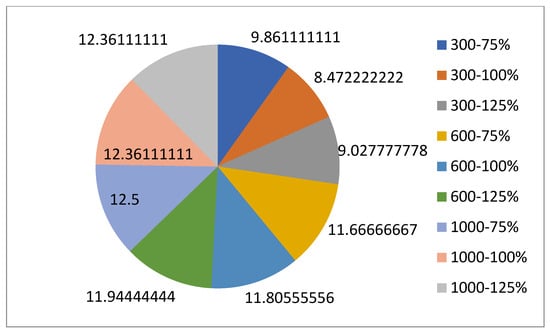
Figure 29.
Population/generations contribution in instances: SUS W.
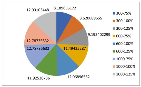
Figure 30.
Population/generations contribution in instances: SUS.
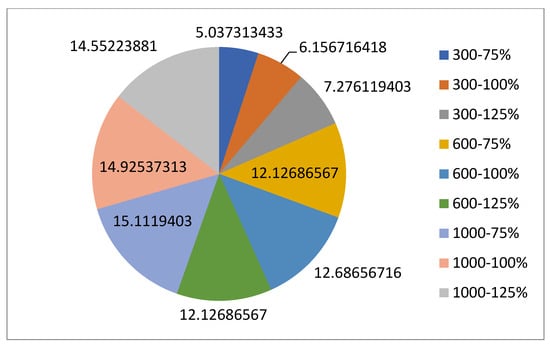
Figure 31.
Population/generations contribution in instances: TOURN W.
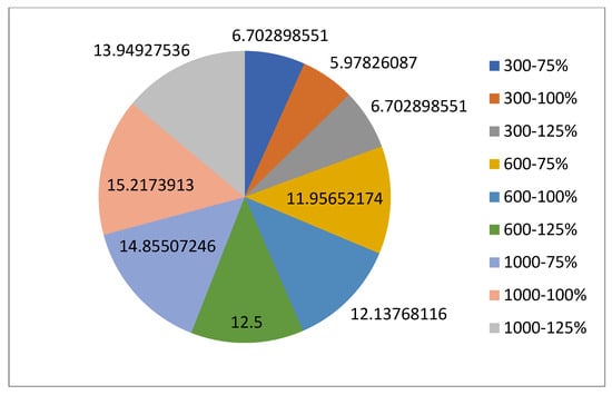
Figure 32.
Population/generations contribution in instances: TOURN.
6.2. Uncertain Case Results
For the uncertain case, the results are discussed per section. As mentioned earlier, there are three sections for discussion, each tackling a different point. For each parent selection method tested, a total of 1080 instances were recorded, which makes the total number of instances for all four parent selection methods 4320 instances. For the line plots used throughout this section, the best scoring instances recorded for each population and number of generations were used to plot the data.
6.2.1. First Experimental Phase
The first section had the purpose of having the nearest value to reach the global minimum possible. The number of blanks has also been recorded. In the literature, the acceptable results regarding the accuracy of the model are a variation of 5% from the global minimum. The global minimum is known to be USD 9110.475. Figure 33, Figure 34, Figure 35 and Figure 36 show line charts comparing each parent selection method in terms of fitness score. The results show that with the increase in the population size, the result is closer to the acceptable level. However, it is shown that TOURN and TOURN W are superior to the results for SUS and SUS W. This can be affiliated with tournament being less sensitive to stochastic noise. With the scale of the model increasing in comparison to the normal case, the effect of the stochastic noise more significantly affects the performance of SUS as a parent selection technique.
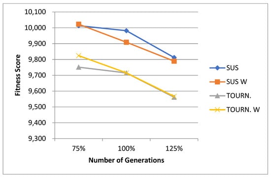
Figure 33.
Best fitness scores per parent selection method for a population of 300.
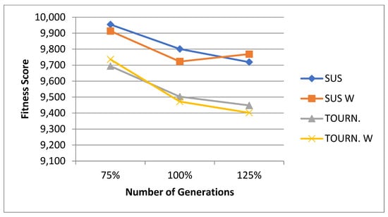
Figure 34.
Best fitness scores per parent selection method for a population of 600.
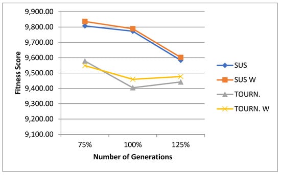
Figure 35.
Best fitness scores per parent selection method for a population of 1000.
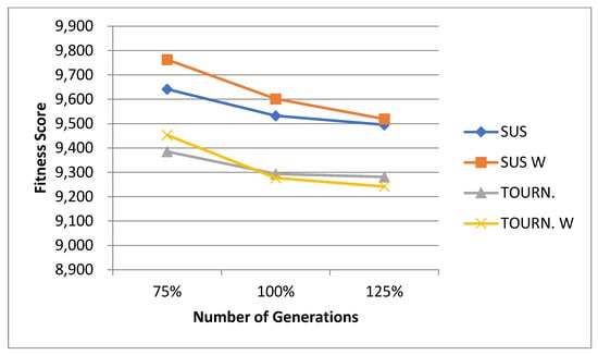
Figure 36.
Best fitness scores per parent selection method for a population of 3000.
The best fitness value achieved was by TOURN W, with a fitness score of USD 9241.876. In terms of accuracy, this is an error of 1.41%, which is well within the benchmark set in the literature. For TOURN, it was able to achieve a score within the 5% error starting from a population size of 300 at 125% number of generations. However, this result is relatively on the border of the 5% figure, meaning that it may vary across multiple runs. As a result, it can be said that TOURN and TOURN W were able to achieve a result within the error range starting from a population size of 600 and a number of generations of 100%. On the other hand, SUS and SUS W were able to achieve a value within the error range starting from a population size of 3000. For SUS, it was able to achieve a value within the error range starting from 100%. Similarly to TOURN, this value is on the border of the error range; hence, it is safer to start at a higher number of generations. As a result, it can be concluded that SUS and SUS W were able to achieve a score within the error range, starting from 125%.
The second factor to consider would be the computational time. For TOURN and TOURN W, the computational time for a single iteration is around 3 min. However, for SUS and SUS W, a very high computational time of approximately 13 min was recorded. While it is normal behavior for SUS to take a long time to achieve a score due to its random nature, it shows the superiority of tournament in this aspect. For the crossover method, it was found that one-point and two-point were the best methods to use, with uniform performing poorly. The application of elitism seems to have no significant effect on the results produced. This can be seen in Figure 33, Figure 34, Figure 35 and Figure 36, where the line charts show very close values achieved between the hybrid techniques and the normal techniques. The values seen are interchangeable with each other, as per the level tested. This means that, for example, at a population size of 300 and number of generations of 100%, the fitness score for SUS is lower than SUS W, while for a population size of 600 and number of generations of 100%, the fitness score for SUS W is lower than SUS. This could be attributed to the random nature of the algorithm itself. It is expected that there would not be a consistent result across all populations and generations. Figure 33 shows a line chart for a population of 300, and Figure 34 shows a line chart for a population of 600. Figure 35 shows a line chart for a population of 1000 and Figure 36 shows a line chart for a population of 3000.
The random nature of the algorithm is also shown using Figure 37, Figure 38, Figure 39 and Figure 40. The figures show box plots for each parent selection method against the population size and generations used. The sample used for each box is the best fitness score achieved from each level tested. From the figures, it can be seen that there is an overall trend in the data where the mean of each sample decreases with an increase in population size. With an increase in the population size, the probability for the algorithm to find a better solution increases, justifying the decrease in the mean value. There is no other consistent trend when describing how the data are plotted. For example, each box is a different size from the other boxes, and the length of the whiskers varies from one box to the other. This supports that the data are unbiased since there is no general trend visible. Another feature that can be seen across all four figures is that the mean value of the results when tested at a 125% number of generations for a certain number of populations is always lower than the consecutive number of populations at a 75% number of generations. This can be explained by the ability of the algorithm to reach a better result, as it has more time to converge given that the number of generations is the termination criteria. When comparing Figure 37 and Figure 38, which are the box plots for SUS and SUS W, it can be seen that there is no clear trend that can be interpreted from both plots. For example, the box size for SUS W is bigger than the box size for SUS at 600–125%; at the same time, the box size for SUS W is smaller than the box size for SUS at 3000–100%. This implies that it is more relatable to the random nature of the algorithm. Furthermore, elitism was used as a hybrid parent selection technique. Similar trends could be seen in Figure 39 and Figure 40 showing the box plots for TOURN and TOURN W.

Figure 37.
Box plot for SUS W.

Figure 38.
Box plot for SUS.
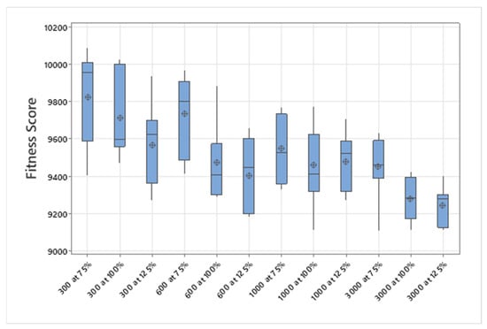
Figure 39.
Box plot for TOURN W.
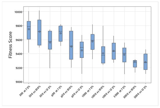
Figure 40.
Box plot for TOURN.
For the number of blanks recorded in the trials, SUS and SUS W recorded a very high number in comparison to the ones recorded by TOURN and TOURN W. SUS W recorded the highest value of 186, followed by SUS, at 152 blanks. TOURN W recorded 75 blanks, followed by 62 blanks for TOURN. It can be seen that elitism had an effect on the stability of the results in terms of the algorithm being able to converge within the allowed number of generations. Figure 41 shows a bar chart comparing the number of blanks produced by each parent selection method. Further analyzing the data, it was found that across all nine trials combining the crossover technique with the percentages of crossover and mutation, the highest number of blanks recorded was the one utilizing uniform as a crossover method. This can be interpreted by the fact that uniform enhances the exploration of the genetic algorithm, regardless of the parent selection technique. Hence, the number of blanks recorded produced by uniform is higher in comparison to the ones produced by one-point and two-point crossover methods. This shows that one-point and two-point methods encourage exploitation more than exploration. Figure 42, Figure 43, Figure 44 and Figure 45 show pie charts presenting the percentage contribution of the trials to the number of blanks.

Figure 41.
Number of blanks per parent selection method.
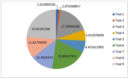
Figure 42.
Contribution of trials in blanks: SUS W.
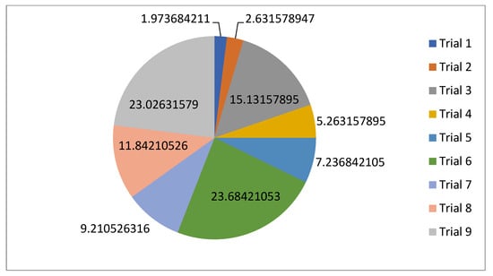
Figure 43.
Contribution of trials in blanks: SUS.
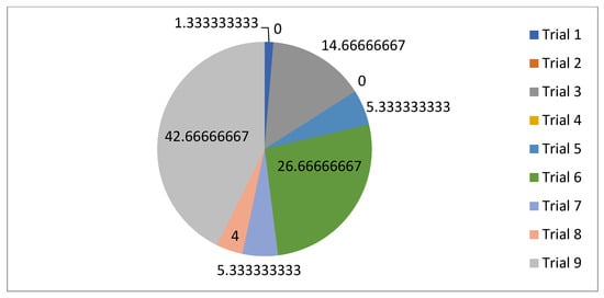
Figure 44.
Contribution of trials in blanks: TOURN W.
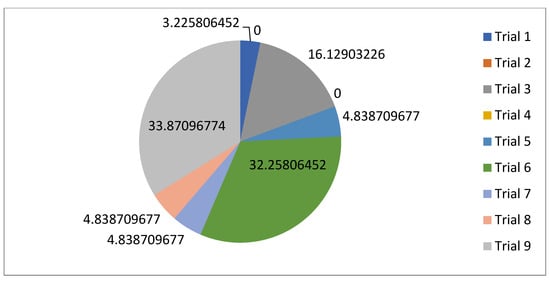
Figure 45.
Contribution of trials in blanks: TOURN.
For the effect of the population size with the number of generations, it was found that the highest number of blanks was recorded by the lowest number of generations, which is 75%. This is consistent across all population sizes. This can be attributed to 75% of the population size being used as a number of generations, which is not enough time for the algorithm to find a result that would be lower than the fitness value that the algorithm started with. This result is consistent across all four parent selection methods. Figure 46, Figure 47, Figure 48 and Figure 49 show pie charts demonstrating the contribution of the population size and number of generations per parent selection method.
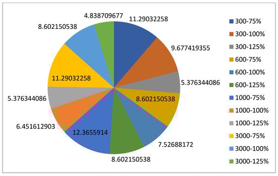
Figure 46.
Population/generation contribution in blanks: SUS W.
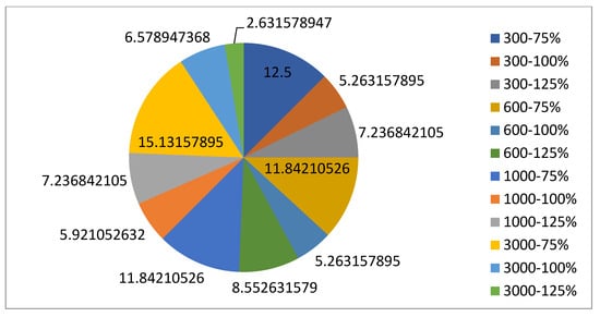
Figure 47.
Population/generation contribution in blanks: SUS.

Figure 48.
Population/generation contribution in blanks: TOURN W.
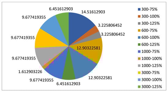
Figure 49.
Population/generations contribution in blanks: TOURN.
6.2.2. Second Experimental Phase
Based on the results of the first section, it was determined that the effect of elitism on the fitness score is insignificant. However, the experimentation continued utilizing elitism as a hybrid technique for results enhancement. The results show that TOURN remained the better parent selection method across the different population sizes. The best fitness score was achieved by TOURN with a population size of 3000 at level 300% of USD 9114.492 with an error of 0.044%. The best result achieved by SUS was also with a population size of 3000 at level 300% at USD 9171.906. This result was achieved with an error of 0.66%. With very close results reached, the computational time is taken into consideration. The computational time taken by TOURN was approximately 7 min. In comparison to SUS, it was found to be superior in terms of time than SUS, taking approximately 25 min to converge.
The results also show that for the smallest population size of 300, there is a significant improvement in the results between levels 125% and 200%. Between the levels of 200 and 300%, the behavior shifts, with the fitness score increasing. This behavior is seen in both parent selection methods. While this behavior could be explained by the random nature of the algorithm, it is worth investigating further to make sure that the behavior is not explicit to small-sized populations. For the remainder of the population sizes, the behavior is relatively consistent. Figure 50, Figure 51, Figure 52 and Figure 53 show line plots of the data.
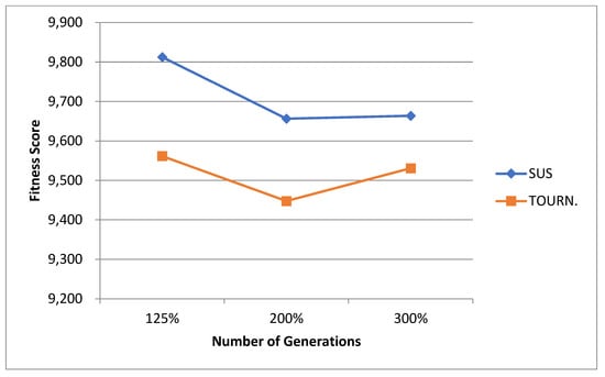
Figure 50.
Best fitness score per parent selection method: population of 300.
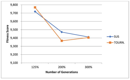
Figure 51.
Best fitness score per parent selection method: population of 600.
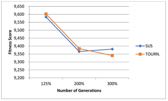
Figure 52.
Best fitness score per parent selection method: population of 1000.
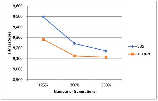
Figure 53.
Best fitness score per parent selection method: population of 3000.
For the comparison between the population sizes and the number of generations, it was found that the smaller population size of 300% would surpass the next largest population size at 125%. This shows that given enough time to converge, small population sizes are more capable of producing reliable results than increasing the population size. This behavior was found to be consistent across both parent selection methods, with the exception of TOURN at 1000 at 125% against 3000 at 125%. This is an anomaly in the data since the behavior is consistent across both parent selection methods. Further analysis was made by retrying this specific level to show whether it would change. The result was consistent with the initial trial. It might need further investigation and experimentation with larger population sizes to see whether this anomaly can be attributed to the randomness of the algorithm or if it is the behavior itself that shifts after a certain population size. Table 5 shows the comparison between each population size at larger number of generations against the second largest population size with the lower number of generations for SUS. Table 6 shows the comparison between each population size at a larger number of generations against the second largest population size with the lower number of generations for TOURN.
Table 5.
Comparison between population size and number of generations: SUS.
Table 6.
Comparison between population size and number of generations: TOURN.
6.2.3. Third Experimental Phase
For the change in the number of elites, both parent selection methods show that changing the number of elites did not have a significant effect in terms of the fitness score and RMSE. The fitness score changed with an average of USD 100 across all levels tested; this can be translated into a 1% change in the overall cost. This is deemed an insignificant result since the behavior across all population sizes varies due the random nature of the algorithm. The RMSE also exhibited the same behavior as the fitness score. While the change in the RMSE was more significant than the fitness score, the random behavior can still be seen and the RMSE itself is within the acceptable level. Figure 54 and Figure 55 show the change in the fitness score for SUS for population sizes of 300 and 3000, and Figure 56 and Figure 57 also show the change in the RMSE for SUS. Figure 58 and Figure 59 show the change in the fitness score for TOURN for population sizes of 300 and 3000, and Figure 60 and Figure 61 also show the change in the RMSE for TOURN.

Figure 54.
Effect on fitness score: SUS 300.
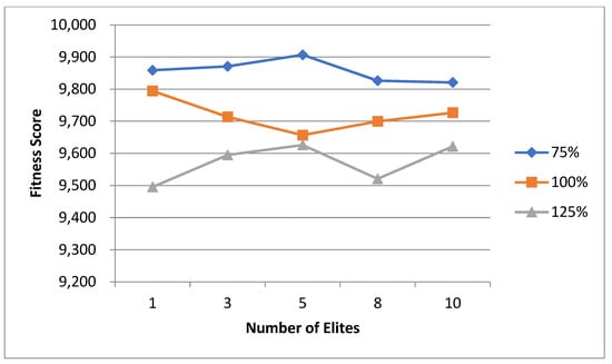
Figure 55.
Effect on fitness score: SUS 3000.
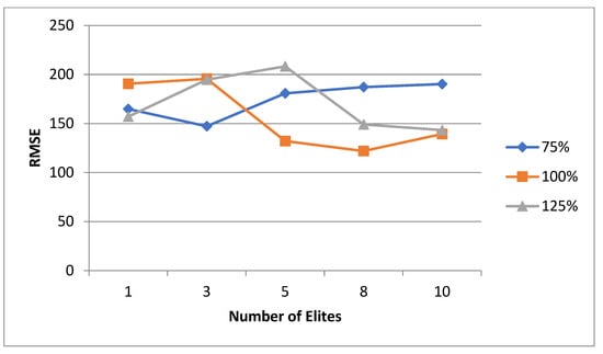
Figure 56.
Effect on RMSE: SUS 300.
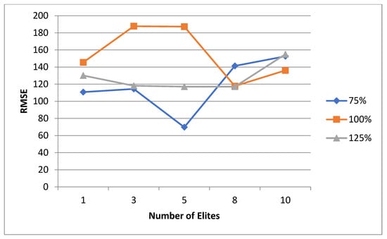
Figure 57.
Effect on RMSE: SUS 3000.
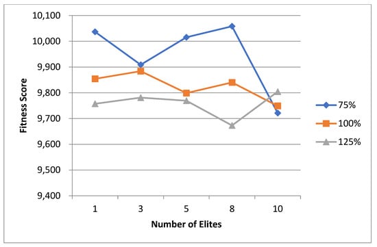
Figure 58.
Effect on fitness score: TOURN 300.
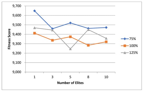
Figure 59.
Effect on fitness score: TOURN 3000.
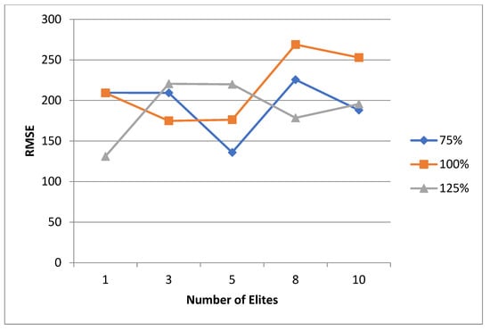
Figure 60.
Effect on RMSE: TOURN 300.
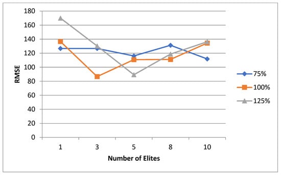
Figure 61.
Effect on RMSE: TOURN 3000.
6.3. Variable Selection Outlook
For the smaller model tackling the normal case, it is recommended to use SUS as the parent selection method at a population of 600 and a number of generations equal to 75% of the population size. For the crossover technique, any of the three methods tried for crossover will deliver the required result. For the percentages between crossover and mutation, any of the three levels will also be acceptable for a satisfying result. If tournament is the parent selection method to use, it is recommended to increase the population size to 1000 to produce satisfactory results. The same is utilized for the crossover methods and the percentages used for SUS can be utilized for tournament. These recommendations are made in a real-life case; the global minimum is unknown, and hence the number of instances cannot be tested.
For the larger model tackling the uncertain case, it is recommended to use tournament as the parent selection method. The recommendation is to first try at a 1000 population size and at 125% value for the number of generations. It is recommended to first test one-point and two-point as crossover methods, and use 90–10% and 80–20% as the percentages for crossover and mutation of the parents. Afterwards, it is recommended to determine which variables produced the best results and then test at 200% as the number of generations. If a hybrid technique is used, a single elite would suffice for an acceptable result. For a model of that size, the usage of these variables and applying the proposed methodology would ensure the production of a satisfactory result within the allowed error range.
6.4. General Discussion
Overall, the results produced by the genetic algorithm have shown that the implementation of social aspects is possible through the concept of monetary penalties. This has proven that social aspects are not limited in implementation to “job creation” and “community development”. The in-depth analysis of the variables gives an insight into where to start when experimenting with the genetic algorithm. The variables tackled and recommended are for models of the sizes tackled in this article. It is recommended to expand the model by increasing the number of locations and expanding the model boundaries to include other areas of improvement. These areas may include the production system. This expands the model boundaries beyond the distribution system to include what happens within the facility itself. An example for the expansion of the model can be seen from Yushuang Hou et al., where the authors developed a multi-objective brain storm algorithm to maximize the processing quality and minimize tardiness [56]. This opens further research directions to determine what social aspects can be introduced to the production system. In that case, the employees would be the focus of the social aspects. Since expanding the model is the preferable research direction, it is recommended to test the genetic algorithm to determine whether it would perform under the new boundaries. It is also recommended to use a hybrid technique of the optimizer and reinforcement learning methods, such as the one utilized by Behrang Bootaki and Guoqing Zhang [51]. A recent study conducted by Yaping Fu et al. shows that there is a significant increase in the utilization of hybrid techniques where an optimizer is joined with a reinforcement learning technique to solve large-scale problems [57]. Yushuang Hou et al. showed the strength in the concept of hybridization when developing a Q-learning-based multi-objective evolutionary algorithm to tackle an optimization problem covering both the production system and the distribution system [58]. Another example for the hybridization of algorithms is given by Zhengpei Zhang et al., who developed an artificial bee colony algorithm that utilizes Q-learning within the model to strengthen the exploration and exploitation [59].
7. Conclusions
This study aimed at integrating the social pillar of sustainability in solving a capacitated two-echelon location-routing problem for SMEs using optimization technology. The technology used was a genetic algorithm which tackled two models of different sizes; one tackling the normal demand case, and the other tackling a case of uncertainty. The study focused on introducing social aspects of sustainability to the problem from aspects that, to the authors’ knowledge, have not been tackled before. These aspects are introducing breaks for the driver and the proximity to a transportation hub as monetary penalties. This has proved to be successful in implementation. The study also aimed to shed light on the process of experimenting on the algorithm, since this is overlooked in the literature. This process was made as a part of refining the results produced by the algorithm and providing an insight for future research on which variables to start with that would guarantee a satisfying result. The algorithm tackled a problem of the authors’ design that induced stochastic noise. The algorithm was successful in solving the problem with an accuracy of 99.956%. The study showed that tournament performed better than SUS as a parent selection method, since tournament is less sensitive to stochastic noise. The study also showed that when tackling a problem of that size, elitism had no significant effect on the result achieved as a hybrid parent selection technique. When discussing the number of elites to use, it was found that the number of elites had no significant effect on either the fitness score or the RMSE. Overall, the study was successful in showing that social factors can be introduced to models further than what is currently being tackled and it opens more research directions to further consider. On a more technical aspect, while the variables selected for the study cannot be generalized to any problem, this gives an insight specifically for LRPs on where to start the experimentation phase, so as not to waste computational time and power.
As a recommendation for future work, the size of the models should be increased to tackle larger-sized problems that are suitable for larger enterprises. It is also recommended to tackle larger population sizes for larger models to determine whether similar behavior could be achieved and to pave the way for future research to produce satisfactory results. Furthermore, comparison of the results of the genetic algorithm with more recent evolutionary algorithms should be performed. More social aspects that can be implemented for both SMEs and larger enterprises need to be considered. It is also recommended to explore other solutions on how to implement social aspects generally. While the concept of monetization has proved its success in LRP, it may not be applicable to other social aspects in other problems. Certain delivery periods can also be introduced to the model since this is closer to the real-life case. By nature, the algorithm was found to target the nearest suppliers and distribution centers to reduce transportation costs. If a handicap is to be introduced, it is recommended to use clustering so that faraway suppliers and distribution centers could also be targeted.
Author Contributions
Conceptualization, M.M. and L.A.S.; methodology, M.N.; software, M.N.; validation, M.N. and M.M.; formal analysis, M.N.; investigation, M.N.; resources, M.M.; data curation, M.N.; writing—original draft preparation, M.N.; writing—review and editing, M.M. and L.A.S.; visualization, M.N.; supervision, M.M. and L.A.S.; project administration, M.M. and L.A.S. All authors have read and agreed to the published version of the manuscript.
Funding
This research received no external funding.
Data Availability Statement
All codes used in this study are publicly available at https://github.com/MohamedMagdy95/LRP-2 (accessed on 23 March 2025).
Acknowledgments
I would like to give a special thank you to Nahla Afifi of the Institute of Medical Systems Biology, University of Ulm for her valuable contribution to this work. Her dedication to the work is unmatched.
Conflicts of Interest
The authors declare no conflicts of interest.
Abbreviations
The following abbreviations are used in this manuscript:
| SDGs | Sustainability Development Goals |
| TBL | Triple bottom line |
| LRP | Location-routing problem |
| VRP | Vehicle-routing problem |
| B2B | Business-to-business |
| B2C | Business-to-customer |
| CLRP | Capacitated LRP |
| 2E-CLRP | Two-echelon capacitated LRP |
| GA | Genetic algorithm |
| SCM | Supply chain management |
| TQM | Total quality management |
| WBCSD | World Business Council for Sustainable Development |
| WACOSS | Western Australian Council of Social Services |
| OECD | Organization for Economic Cooperation and Development |
| SSCs | Sustainable supply chains |
| SBD | Sustainable business development |
| SMEs | Small to medium enterprises |
| B&C | Branch and cut algorithm |
| RMSE | Root mean square error |
| SUS | Stochastic universal sampling hybrid with elitism |
| SUS W | Stochastic universal sampling |
| TOURN | Tournament hybrid with elitism |
| TOURN W | Tournament selection |
| PS | Population size |
| NOG | Number of generations |
| NOE | Number of elites |
| CO | Crossover percentage |
| M | Mutation percentage |
References
- Easterly, W. The trouble with the sustainable development goals. Curr. Hist. 2015, 114, 322. [Google Scholar] [CrossRef]
- Hamilton, K. Measuring sustainability in the UN system of environmental-economic accounting. Environ. Resour. Econ. 2016, 64, 25–36. [Google Scholar] [CrossRef]
- Lopes, R.B.; Ferreira, C.; Santos, B.S. A simple and effective evolutionary algorithm for the capacitated location–routing problem. Comput. Oper. Res. 2016, 70, 155–162. [Google Scholar] [CrossRef]
- Pham, Q.D.; Nguyen, T.H.; Bui, Q.T. Modeling and solving a multi-trip multi-distribution center vehicle routing problem with lower-bound capacity constraints. Comput. Ind. Eng. 2022, 172, 108597. [Google Scholar] [CrossRef]
- Kravchenko, M.; Pigosso, D.C.A.; McAloone, T.C. Towards the ex-ante sustain- ability screening of circular economy initiatives in manufacturing companies: Consolidation of leading sustainability-related performance indicators. J. Clean. Prod. 2019, 241, 118318. [Google Scholar] [CrossRef]
- Padilla-Rivera, A.; Russo-Garrido, S.; Merveille, N. Addressing the social as-pects of a circular economy: A systematic literature review. Sustainability 2020, 12, 7912. [Google Scholar] [CrossRef]
- Roos Lindgreen, E.; Salomone, R.; Reyes, T. Measuring circular economy at the micro level: Is the social dimension included? In Proceedings of the Atti XXIX Congresso Nazionale Di Scienze Merceologiche 2020, Milan, Italy, 13–14 February 2020; pp. 396–403. [Google Scholar]
- Toorajipour, R.; Sohrabpour, V.; Nazarpour, A.; Oghazi, P.; Fischl, M. Artificial Intelligence in Supply Chain Management: A systematic literature Review. J. Bus. Res. 2021, 122, 502–517. [Google Scholar]
- Cerqueria-Streit, J.A.; Endo, G.Y.; Guarnieri, P.; Batista, L. Sustainable Supply Chain Management in the Route for a Circular Economy: An Integrative Literature Review. Logistics 2021, 5, 81. [Google Scholar] [CrossRef]
- Putro, P.A.W.; Purwaningsih, E.K.; Sensuse, D.I.; Suryono, R.R. Model and implementation of rice supply chain management: A literature review. Procedia Comput. Sci. 2022, 197, 453–460. [Google Scholar]
- Ugochukwu, P.; Engström, J.; Langstrand, J. Lean in the supply chain: A literature review. Manag. Prod. Eng. Rev. 2012, 3, 87–96. [Google Scholar]
- Baran, E.; Korkusuz Polat, T. Classification of Industry 4.0 for Total Quality Management: A Review. Sustainability 2022, 14, 3329. [Google Scholar] [CrossRef]
- Arora, R.; Haleem, A.; Arora, P.K.; Kumar, H. Impact of Integrating Artificial Intelligence with IOT-Enabled Supply Chain—A Systematic Literature Review. In Advances in Manufacturing and Industrial Engineering; Lecture Notes in Mechanical Engineering; Singari, R., Mathiyazhagan, K., Kumar, H., Eds.; Springer: Singapore, 2021. [Google Scholar]
- Singh, R.K.; Kumar, R. Strategic issues in supply chain management of Indian SMEs due to globalization: An empirical study. Benchmarking Int. J. 2020, 27, 913–932. [Google Scholar] [CrossRef]
- Stroumpoulis, A.; Kopanaki, E. Theoratical Perspectives on Sustainable Supply Chain Managmenet and Digital Transformation: A Literature Review and a Conceptual Framework. Sustainability 2022, 14, 4862. [Google Scholar]
- Ahmad, S.; Wong, K.Y.; Rajoo, S. Sustainability indicators for manufacturing sectors: A literature survey and maturity analysis from the triple-bottom line perspective. J. Manuf. Technol. Manag. 2019, 30, 312–334. [Google Scholar] [CrossRef]
- Correia, M.S. Sustainability: An overview of the Triple Bottom Line and Sustainability Implementation. Int. J. Strateg. Eng. (IJoSE) 2019, 2, 29–38. [Google Scholar] [CrossRef]
- Mani, V.; Delgado, C. Supply Chain Social Sustainability for Manufacturing; India Studies in Business and Economics; Springer: Berlin/Heidelberg, Germany, 2018. [Google Scholar]
- IUCN; WWF; UNEP. Caring for the Earth, A Strategy for Sustainable Living; WWF: Gland, Switzerland, 1991. [Google Scholar]
- Hill, S.B. Redesigning agro ecosystems for environmental sustainability: A deep systems approach. Syst. Res. Behav. Sci. 1998, 15, 391–402. [Google Scholar] [CrossRef]
- Lafferty, W.M.; Langhelle, O. Towards Sustainable Development: On the Goals of Development-and the Conditions of Sustainability; Springer: Berlin/Heidelberg, Germany, 1999. [Google Scholar]
- Mani, V.; Gunasekaran, A.; Delgado, C. Supply chain social sustainability: Standard adoption practices in Portuguese manufacturing firms. Int. J. Prod. Econ. 2018, 198, 149–164. [Google Scholar] [CrossRef]
- Seuring, S.; Müller, M. From a literature review to a conceptual framework for sustainable supply chain management. J. Clean. Prod. 2008, 16, 1699–1710. [Google Scholar] [CrossRef]
- Ashby, A.; Leat, M.; Hudson-Smith, M. Making connections: A review of supply chain management and sustainability literature. Supply Chain. Manag. Int. J. 2012, 17, 497–516. [Google Scholar] [CrossRef]
- Gunasekaran, A.; Spalanzani, A. Sustainability of manufacturing and services: Investigations for research and applications. Int. J. Prod. Econ. 2012, 140, 35–47. [Google Scholar] [CrossRef]
- Pinar, M.; Cruciani, C.; Giove, S.; Sostero, M. Constructing the FEEM sustainability index: A Choquet integral application. Ecol. Indic. 2014, 39, 189–202. [Google Scholar] [CrossRef]
- Walker, A.M.; Opferkuch, K.; Lindgreen, E.R.; Simboli, A.; Vermeulen, W.J.; Raggi, A. Assessing the social sustainability of circular economy practices: Industry perspectives from Italy and the Netherlands. Sustain. Prod. Consum. 2021, 27, 831–844. [Google Scholar]
- Hervani, A.A.; Nandi, S.; Helms, M.M.; Sarkis, J. A performance measurement framework for socially sustainable and resilient supply chains using environmental goods valuation methods. Sustain. Prod. Consum. 2022, 30, 31–52. [Google Scholar] [CrossRef]
- Nagy, G.; Salhi, S. Location-routing: Issues, models and methods. Eur. J. Oper. Res. 2007, 177, 649–672. [Google Scholar] [CrossRef]
- Yu, X.; Zhou, Y.; Liu, X.F. A novel hybrid genetic algorithm for the location routing problem with tight capacity constraints. Appl. Soft Comput. 2019, 85, 105760. [Google Scholar] [CrossRef]
- Prodhon, C.; Prins, C. A survey of recent research on location-routing problems. Eur. J. Oper. Res. 2014, 238, 1–17. [Google Scholar] [CrossRef]
- Schneider, M.; Drexl, M. A survey of the standard location-routing problem. Ann. Oper. Res. 2017, 259, 389–414. [Google Scholar] [CrossRef]
- Mara, S.T.W.; Kuo, R.J.; Asih, A.M.S. Location-routing problem: A classification of recent research. Int. Trans. Oper. Res. 2021, 28, 2941–2983. [Google Scholar] [CrossRef]
- Wang, Y.; Wang, X.; Wei, Y.; Sun, Y.; Fan, J.; Wang, H. Two-echelon multi-depot multi-period location-routing problem with pickup and delivery. Comput. Ind. Eng. 2023, 182, 109385. [Google Scholar] [CrossRef]
- Soto-Mendoza, V.; Ruiz-y-Ruiz, E.; García-Calvillo, I.; Nucamendi-Guillén, S.; Cardona-Valdés, Y. A location-routing problem for local supply chains. Comput. Ind. Eng. 2023, 183, 109528. [Google Scholar] [CrossRef]
- Tian, X.D.; Hu, Z.H. A branch-and-price method for a two-echelon location routing problem with recommended satellites. Comput. Ind. Eng. 2023, 184, 109593. [Google Scholar] [CrossRef]
- Zabihian-Bisheh, A.; Vandchali, H.R.; Kayvanfar, V.; Werner, F. A sustainable multi-objective model for the hazardous waste location-routing problem: A real case study. Sustain. Oper. Comput. 2024, 5, 1–14. [Google Scholar] [CrossRef]
- Du, J.; Wang, X.; Wu, X.; Zhou, F.; Zhou, L. Multi-objective optimization for two-echelon joint delivery location routing problem considering carbon emission under online shopping. Transp. Lett. 2023, 15, 907–925. [Google Scholar] [CrossRef]
- Shi, Y.; Lin, Y.; Wang, S.; Wen, H.; Lim, M.K.; Li, Y. A simultaneous facility location and vehicle routing problem with recyclable express packaging consideration for sustainable city logistics. Sustain. Cities Soc. 2023, 98, 104857. [Google Scholar] [CrossRef]
- Hajghani, M.; Forghani, M.A.; Heidari, A.; Khalilzadeh, M.; Kebriyaii, O. A two-echelon location routing problem considering sustainability and hybrid open and closed routes under uncertainty. Heliyon 2023, 9, e14258. [Google Scholar] [CrossRef]
- Osorio-Mora, A.; Saldanha-da-Gama, F.; Toth, P. A risk-averse latency location-routing problem with stochastic travel times. Eur. J. Oper. Res. 2025, 321, 837–850. [Google Scholar] [CrossRef]
- Eydi, A.; Shirinbayan, P. Multi-modal and multi-product hierarchical hub location problem with fuzzy demands. Eng. Appl. Artif. Intell. 2023, 123, 106282. [Google Scholar] [CrossRef]
- Prodhon, C. A metaheuristic for the periodic location-routing problem. In Proceedings of the Symposium Operations Research 2007, Saarbrücken, Germany, 5–7 September 2007; pp. 159–164. [Google Scholar]
- Mohamed, I.B.; Klibi, W.; Sadykov, R.; Şen, H.; Vanderbeck, F. The two-echelon stochastic multi-period capacitated location-routing problem. Eur. J. Oper. Res. 2023, 306, 645–667. [Google Scholar] [CrossRef]
- Yıldız, E.A.; Karaoğlan, İ.; Altiparmak, F. An exact algorithm for Two-Echelon Location-Routing problem with simultaneous pickup and delivery. Expert Syst. Appl. 2023, 231, 120598. [Google Scholar] [CrossRef]
- Domínguez-Martín, B.; Hernández-Pérez, H.; Riera-Ledesma, J.; Rodríguez-Martín, I. A branch-and-cut algorithm for the one-commodity pickup and delivery location routing problem. Comput. Oper. Res. 2024, 161, 106426. [Google Scholar] [CrossRef]
- Barbati, M.; Corrente, S.; Greco, S. Multiobjective combinatorial optimization with interactive evolutionary algorithms: The case of facility location problems. EURO J. Decis. Process. 2024, 12, 100047. [Google Scholar] [CrossRef]
- Tan, D.; Liu, X.; Zhou, R.; Fu, X.; Li, Z. A novel multi-objective artificial bee colony algorithm for solving the two-echelon load-dependent location-routing problem with pick-up and delivery. Eng. Appl. Artif. Intell. 2025, 139, 109636. [Google Scholar] [CrossRef]
- Mahmoudi, N.; Sadegheih, A.; Hosseini-Nasab, H.; Zare, H.K. Routing and scheduling decisions for a single-hub same-day delivery network. J. Eng. Res. 2023, 11, 198–211. [Google Scholar] [CrossRef]
- Hu, Q.; Hu, Y.; Li, X. Multi-period emergency facility location-routing problems under uncertainty and risk aversion. Socio-Econ. Plan. Sci. 2024, 96, 102093. [Google Scholar] [CrossRef]
- Bootaki, B.; Zhang, G. A location-production-routing problem for distributed manufacturing platforms: A neural genetic algorithm solution methodology. Int. J. Prod. Econ. 2024, 275, 109325. [Google Scholar] [CrossRef]
- Aleksandrov, M. Fairness and Efficiency in Social Vehicle Routing Problems. Transp. Res. Procedia 2025, 82, 1994–2013. [Google Scholar] [CrossRef]
- Azab, E.; Nafea, M.; Shihata, L.A.; Mashaly, M. A Machine-Learning-Assisted Simulation Approach for Incorporating Predictive Maintenance in Dynamic Flow-Shop Scheduling. Appl. Sci. 2021, 11, 11725. [Google Scholar] [CrossRef]
- Fortin, F.-A.; De Rainville, F.-M.; Gardner, M.-A.; Parizeau, M.; Gagné, C. DEAP: Evolutionary Algorithms Made Easy. J. Mach. Learn. Res. 2012, 13, 2171–2175. [Google Scholar]
- Hurbans, R. Grokking Artificial Intelligence Algorithms; Manning: Greenwich, CT, USA, 2020. [Google Scholar]
- Hou, Y.; Wang, H.; Fu, Y.; Gao, K.; Zhang, H. Multi-Objective brain storm optimization for integrated scheduling of distributed flow shop and distribution with maximal processing quality and minimal total weighted earliness and tardiness. Comput. Ind. Eng. 2023, 179, 109217. [Google Scholar] [CrossRef]
- Fu, Y.; Wang, Y.; Gao, K.; Huang, M. Review on ensemble meta-heuristics and reinforcement learning for manufacturing scheduling problems. Comput. Electr. Eng. 2024, 120, 109780. [Google Scholar] [CrossRef]
- Hou, Y.; Wang, H.; Huang, X. A Q-learning-based multi-objective evolutionary algorithm for integrated green production and distribution scheduling problems. Eng. Appl. Artif. Intell. 2024, 127, 107434. [Google Scholar] [CrossRef]
- Zhang, Z.; Fu, Y.; Gao, K.; Pan, Q.; Huang, M. A learning-driven multi-objective cooperative artificial bee colony algorithm for distributed flexible job shop scheduling problems with preventive maintenance and transportation operations. Comput. Ind. Eng. 2024, 196, 110484. [Google Scholar] [CrossRef]
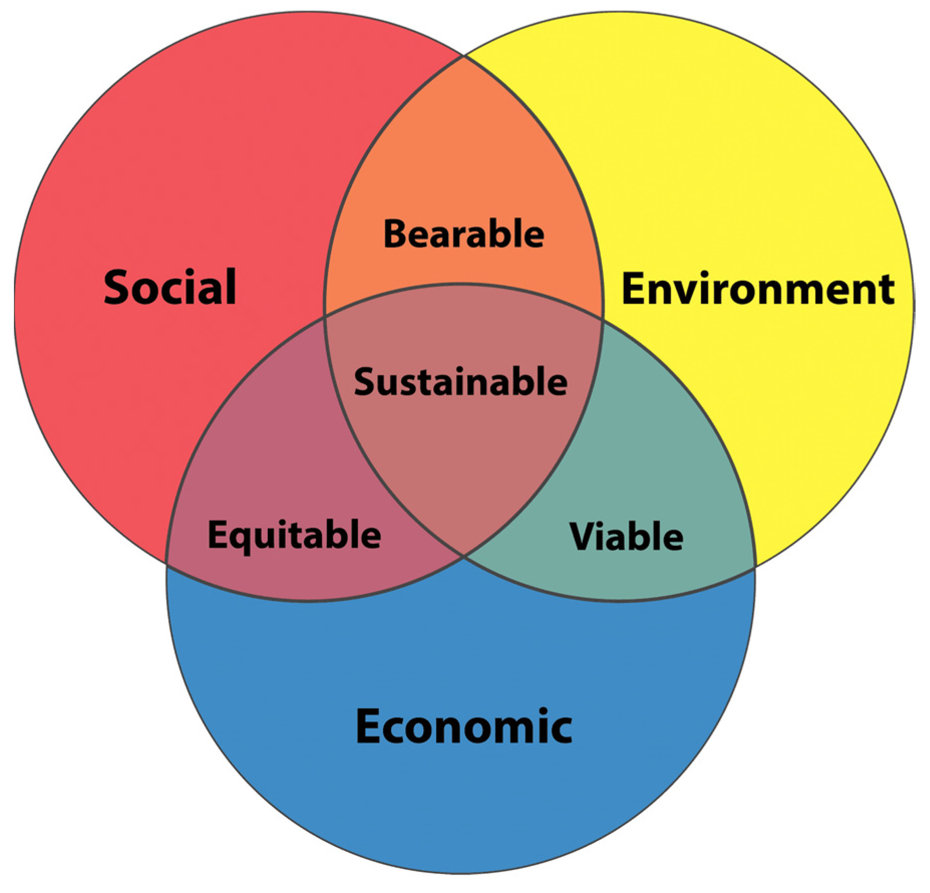
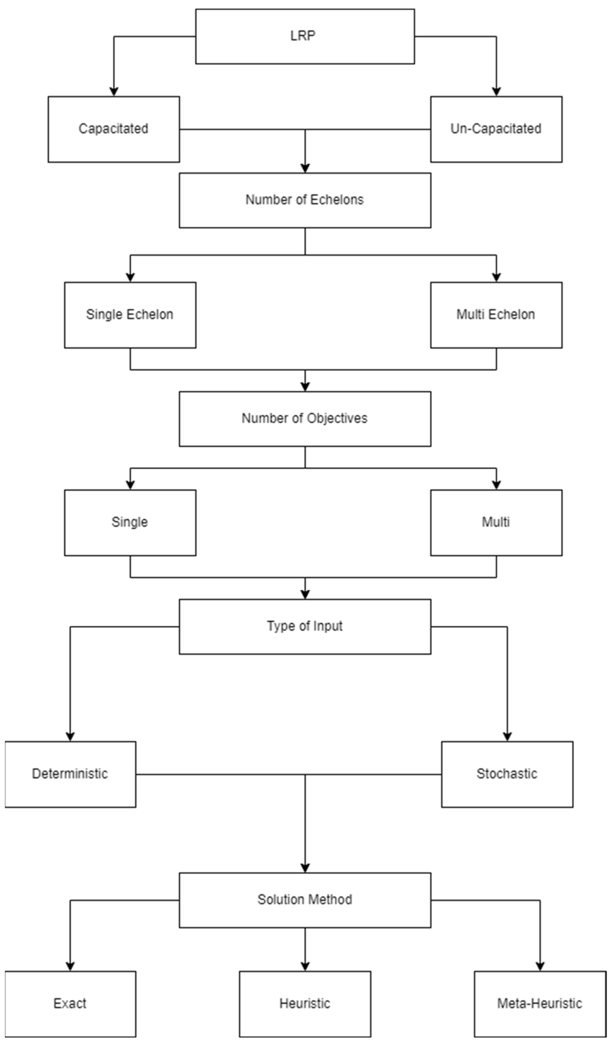
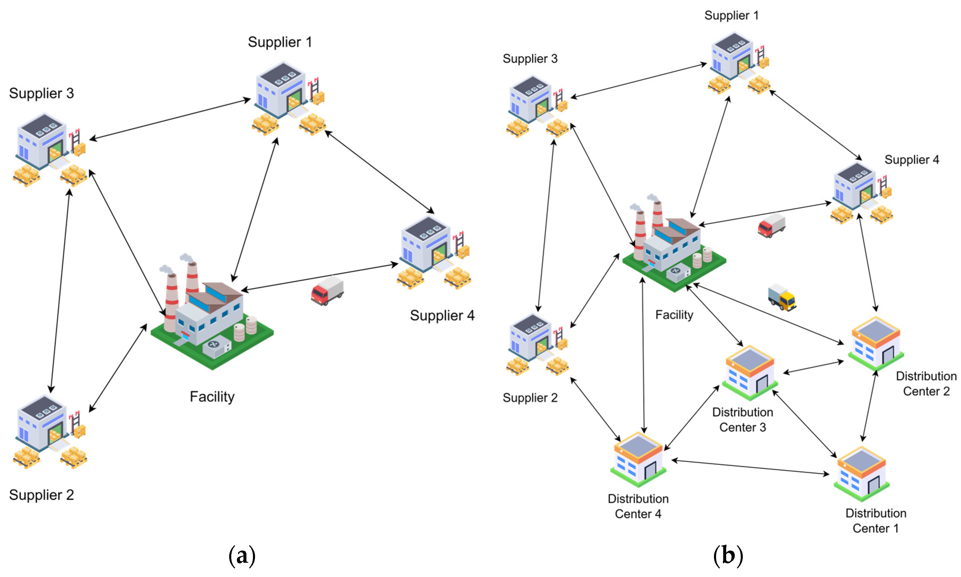
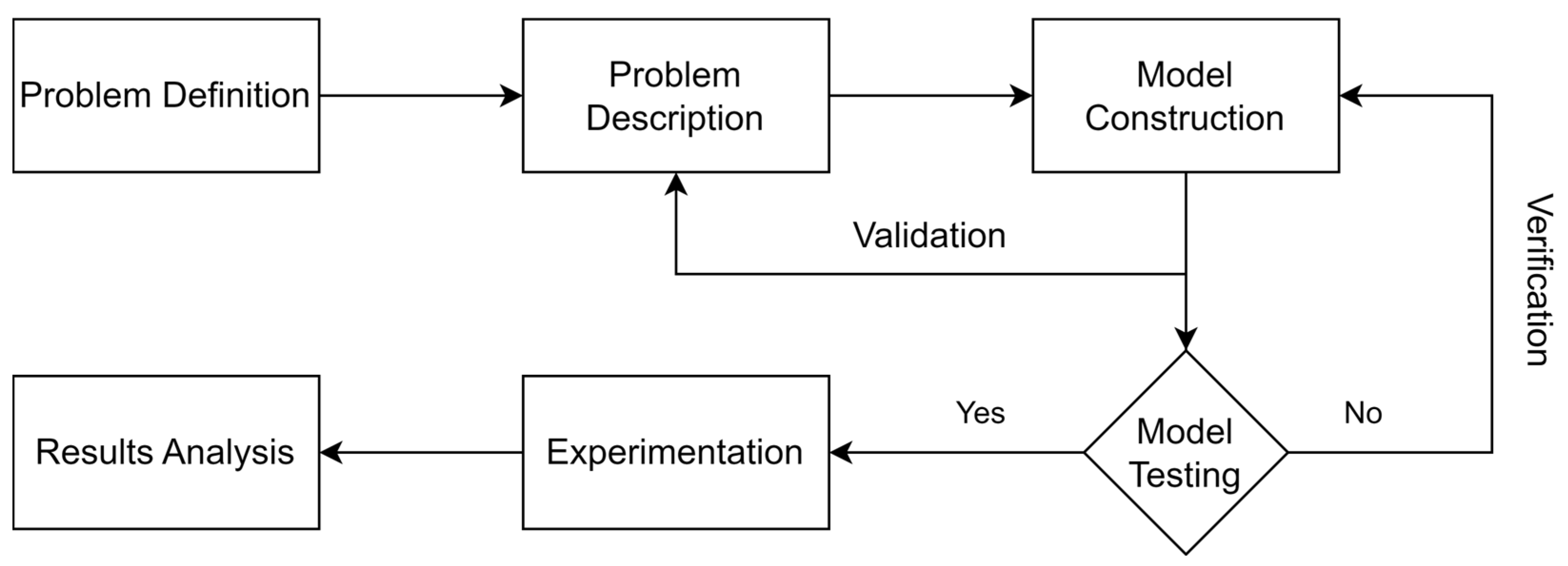
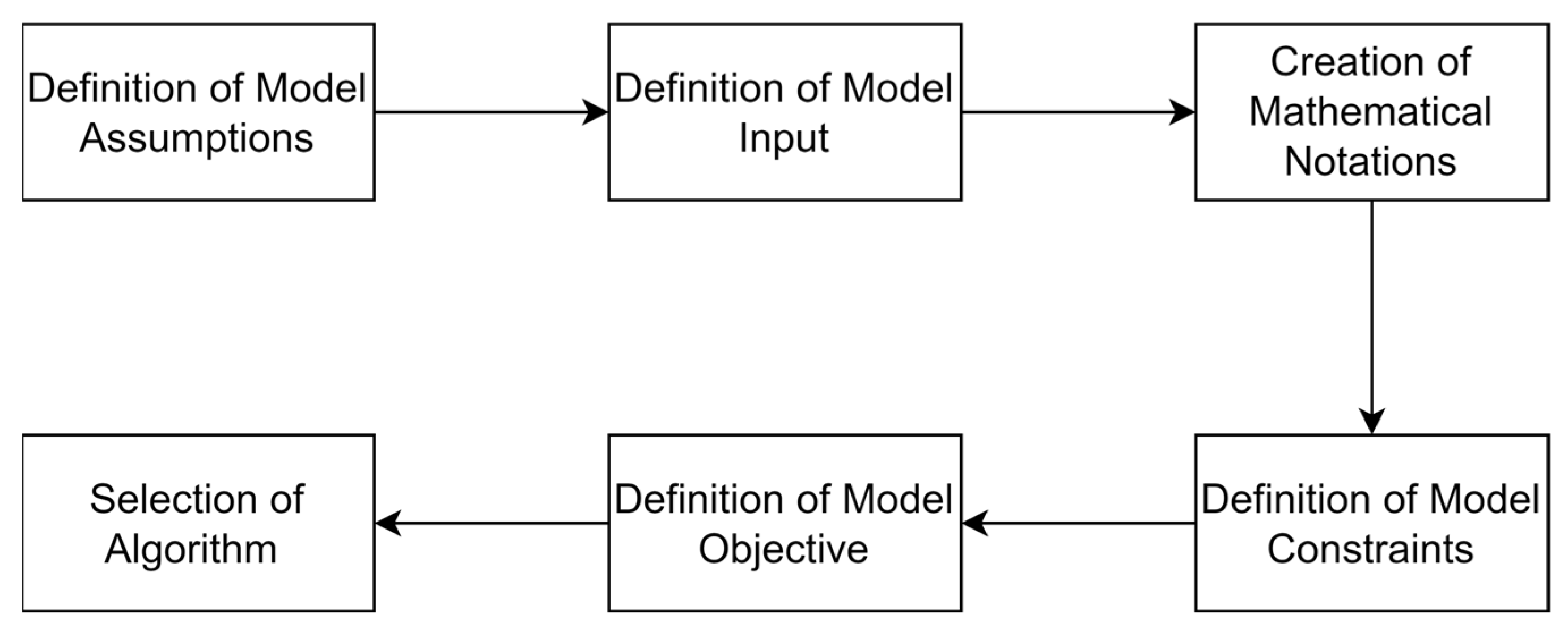

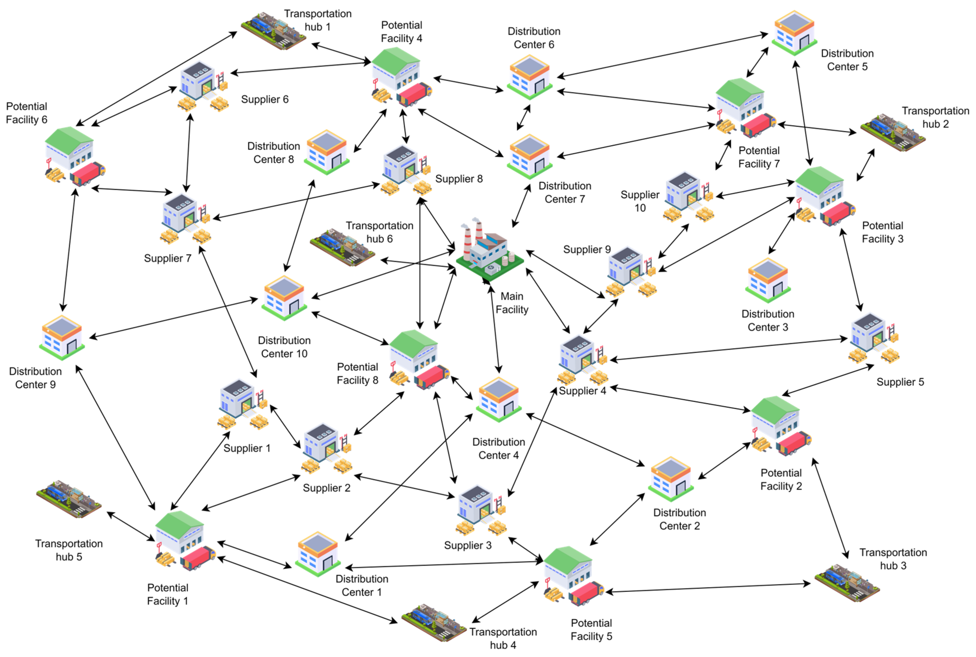

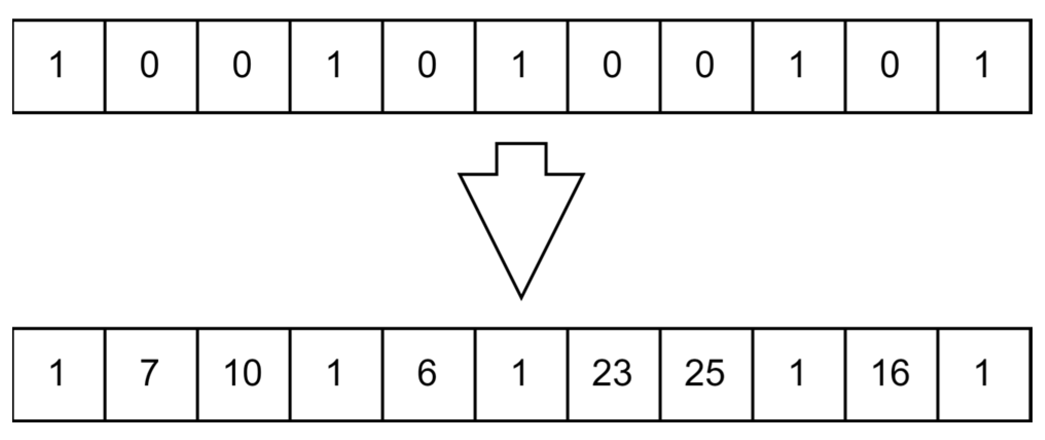
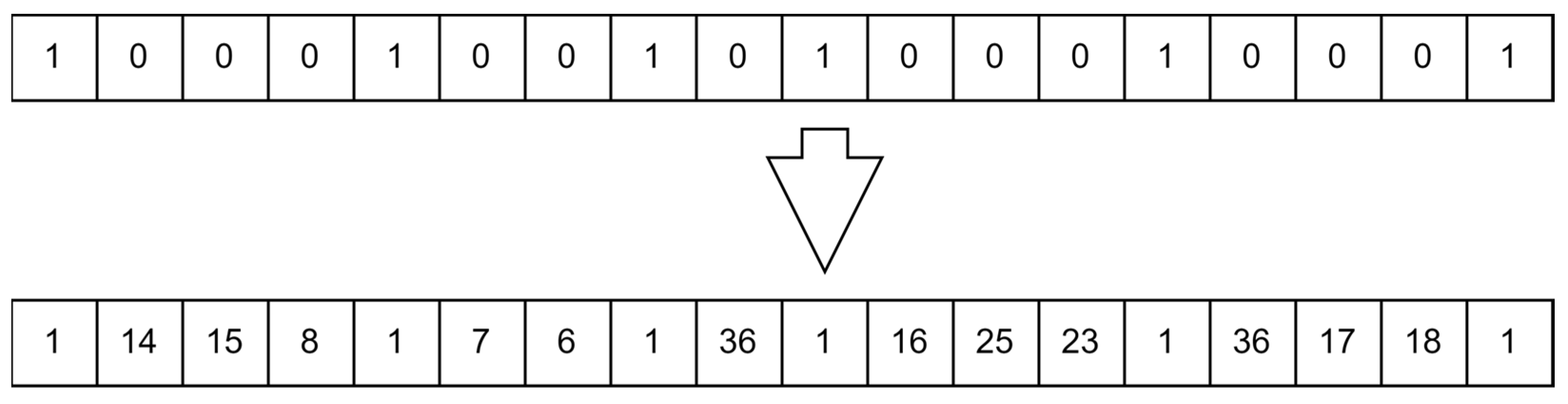
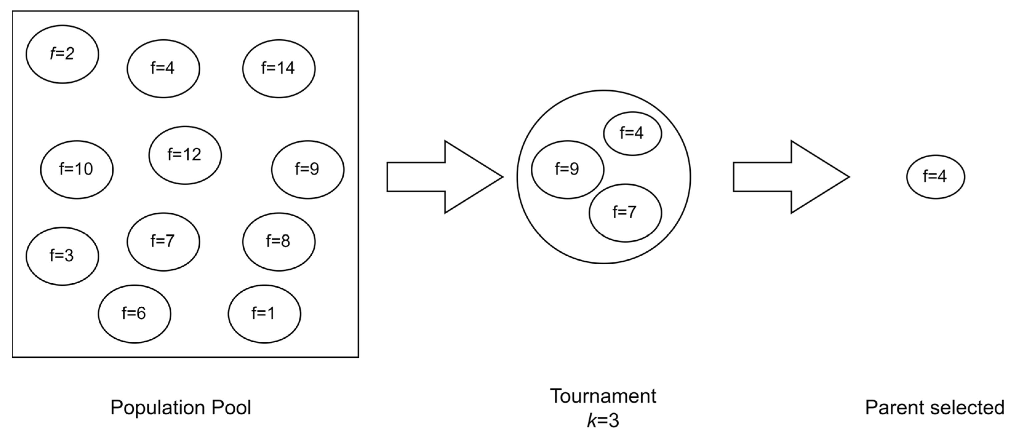
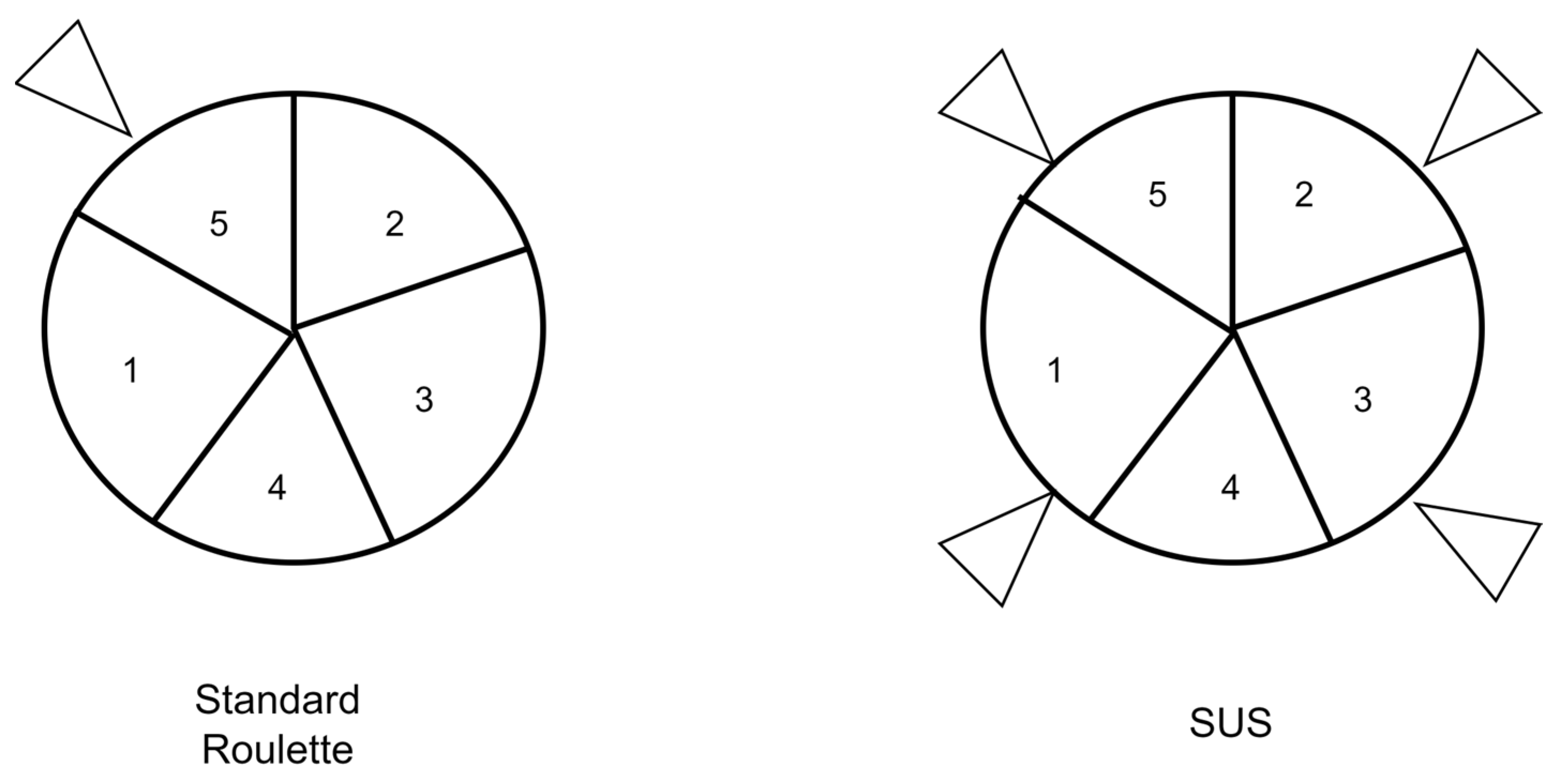

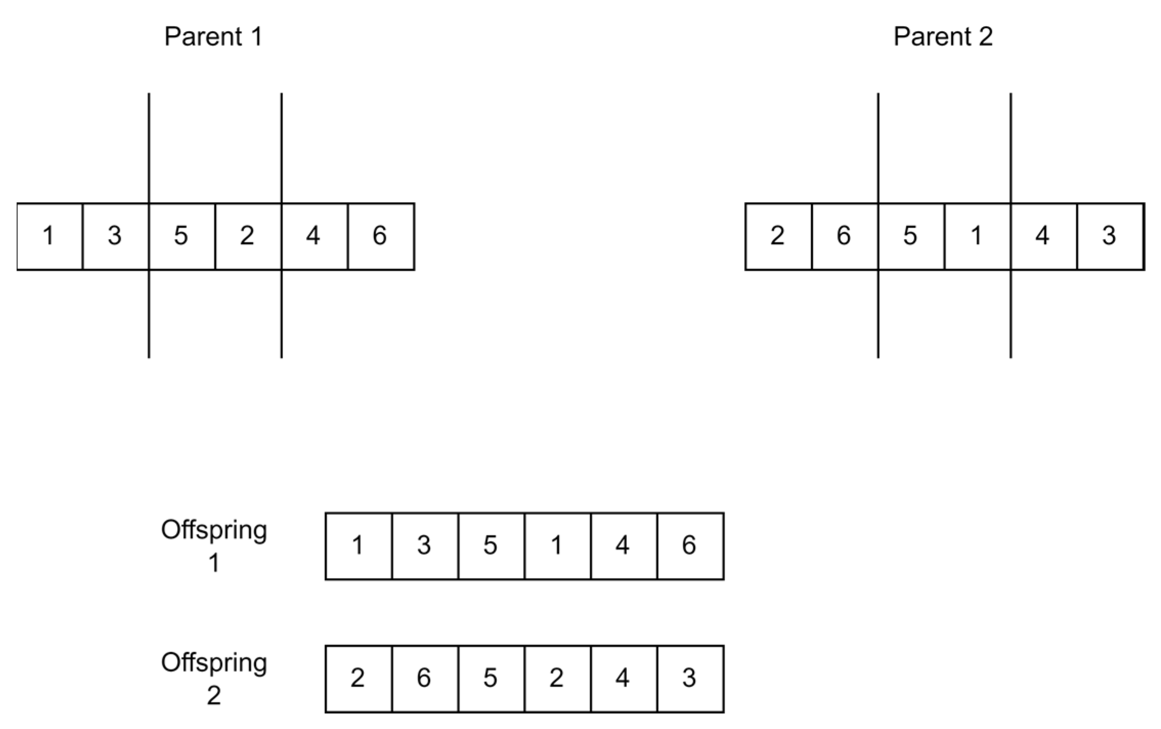
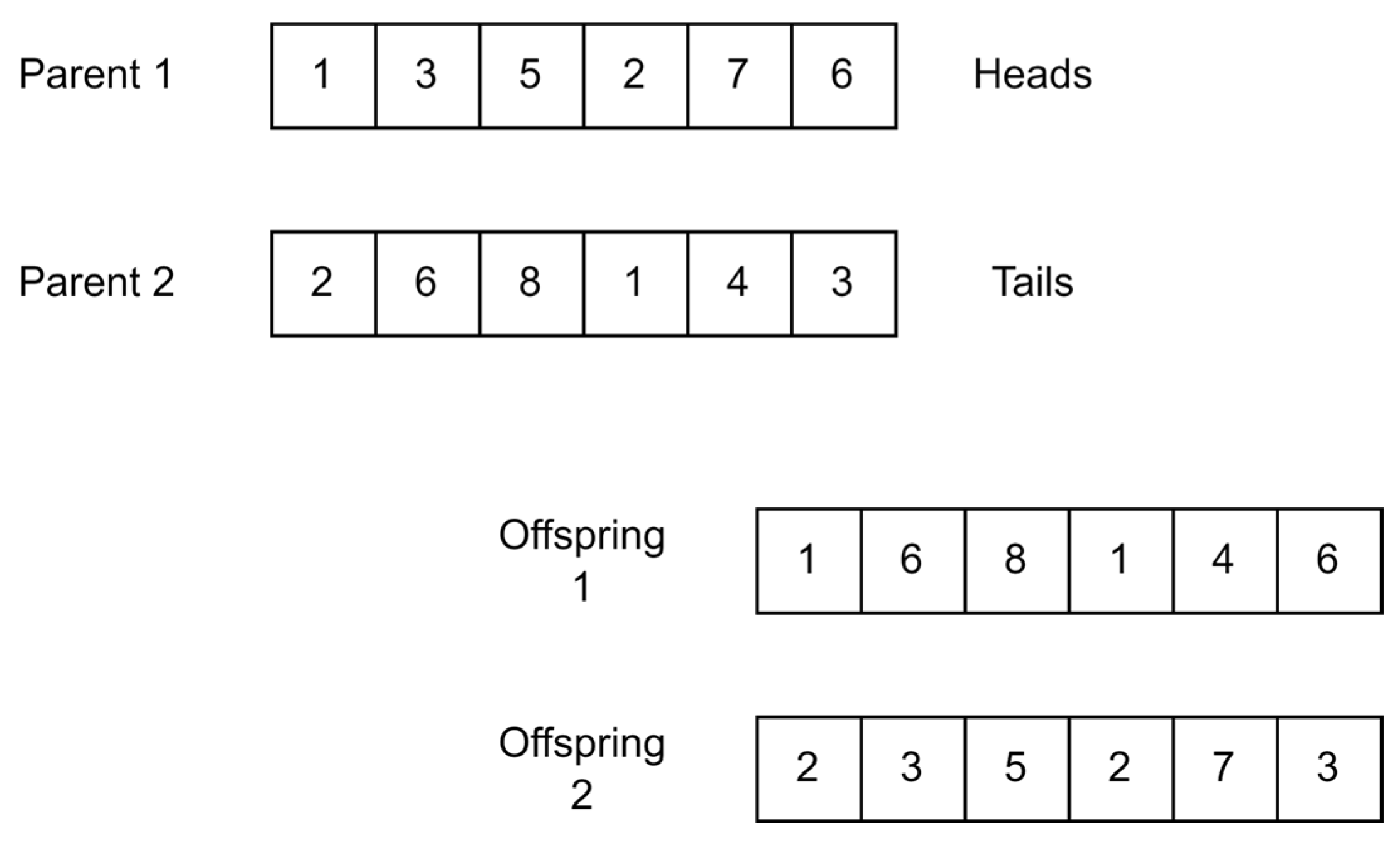
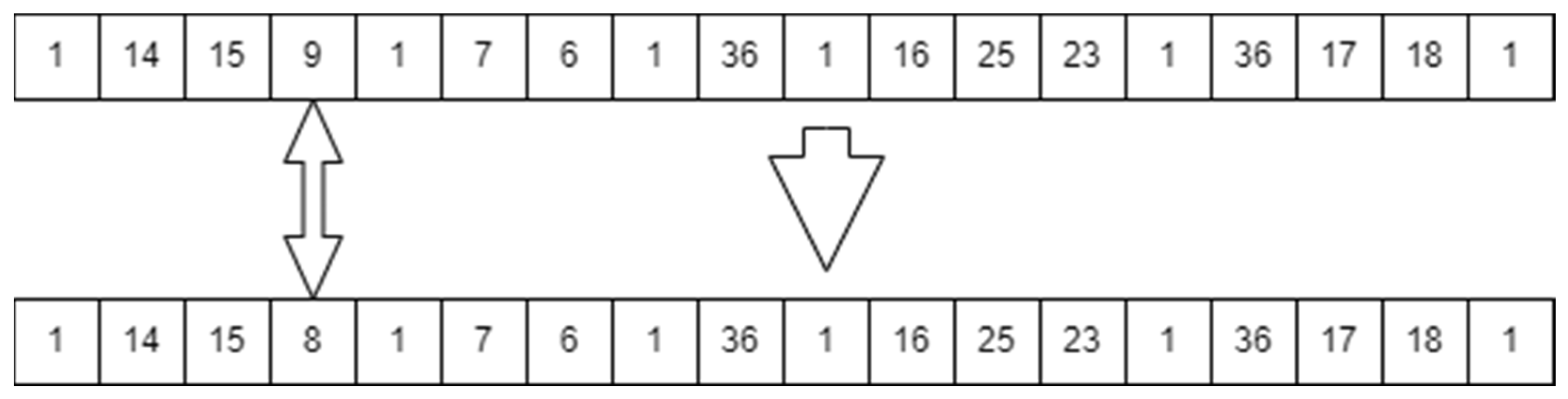
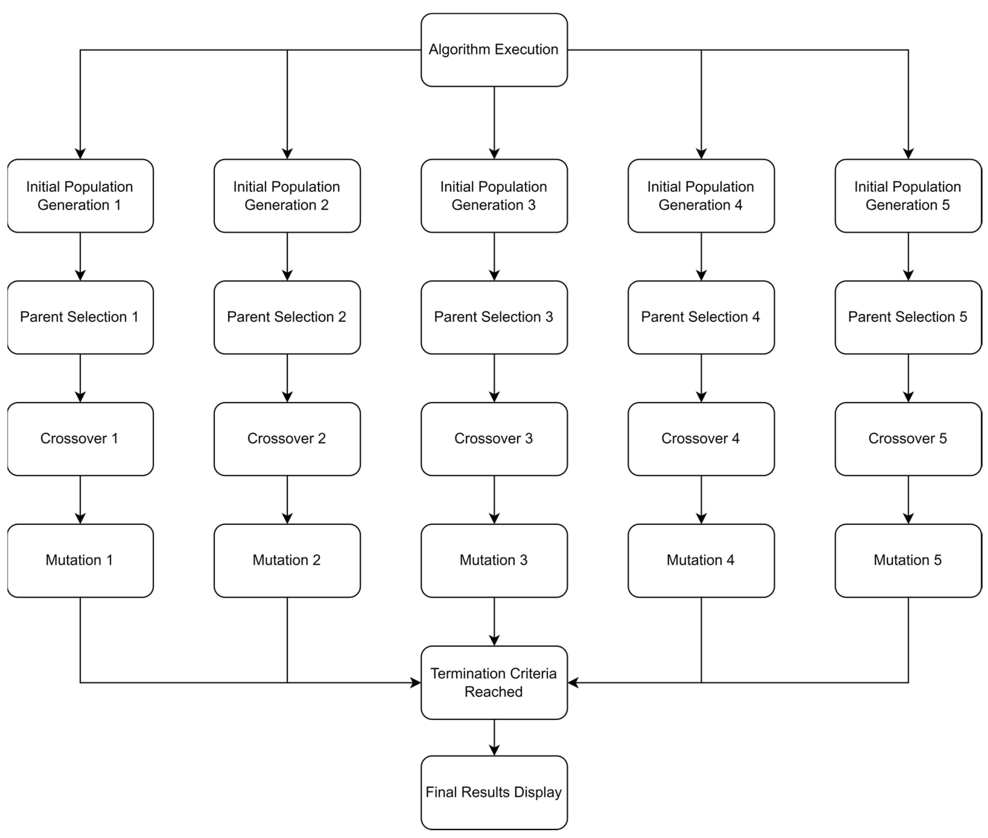


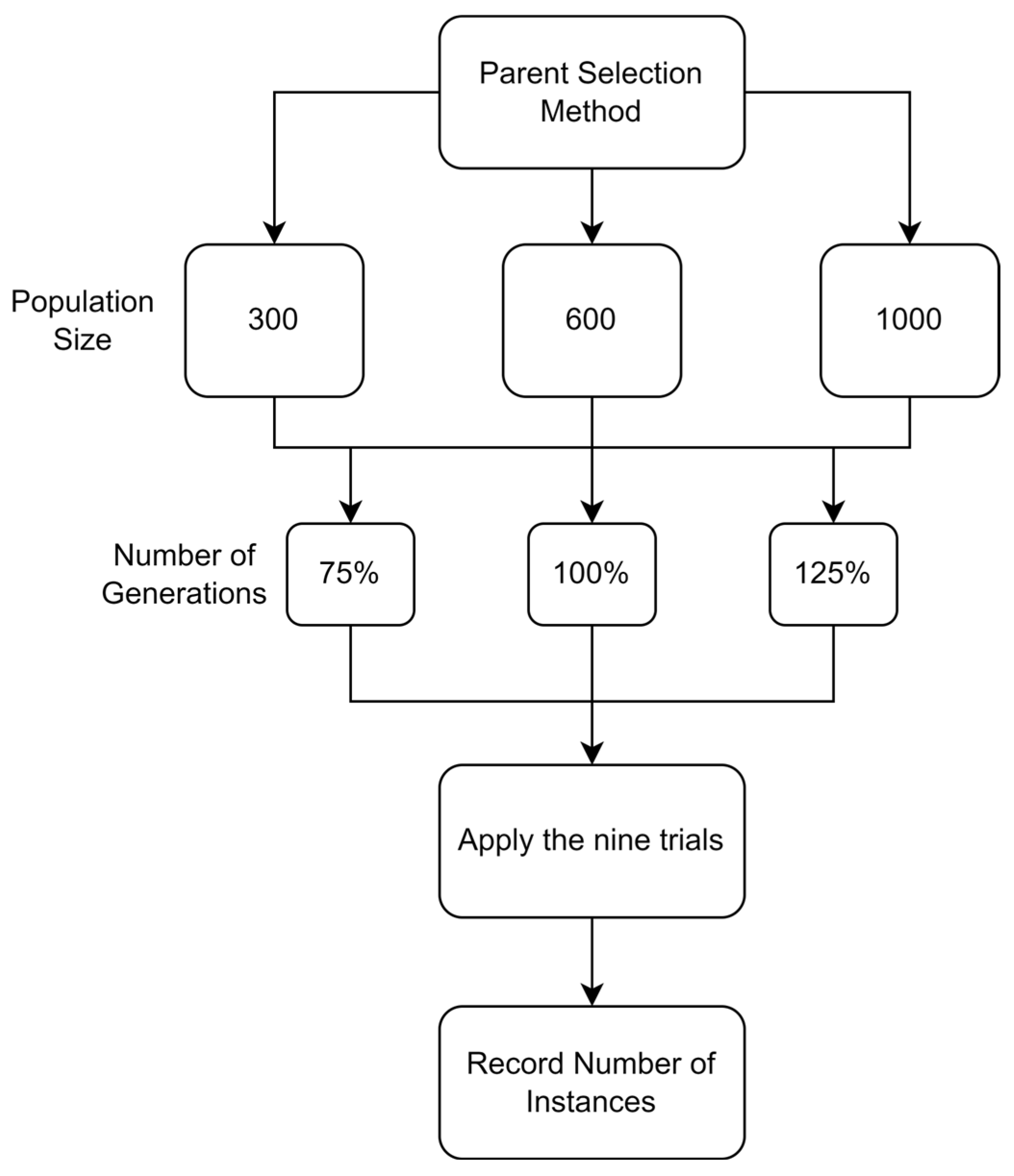
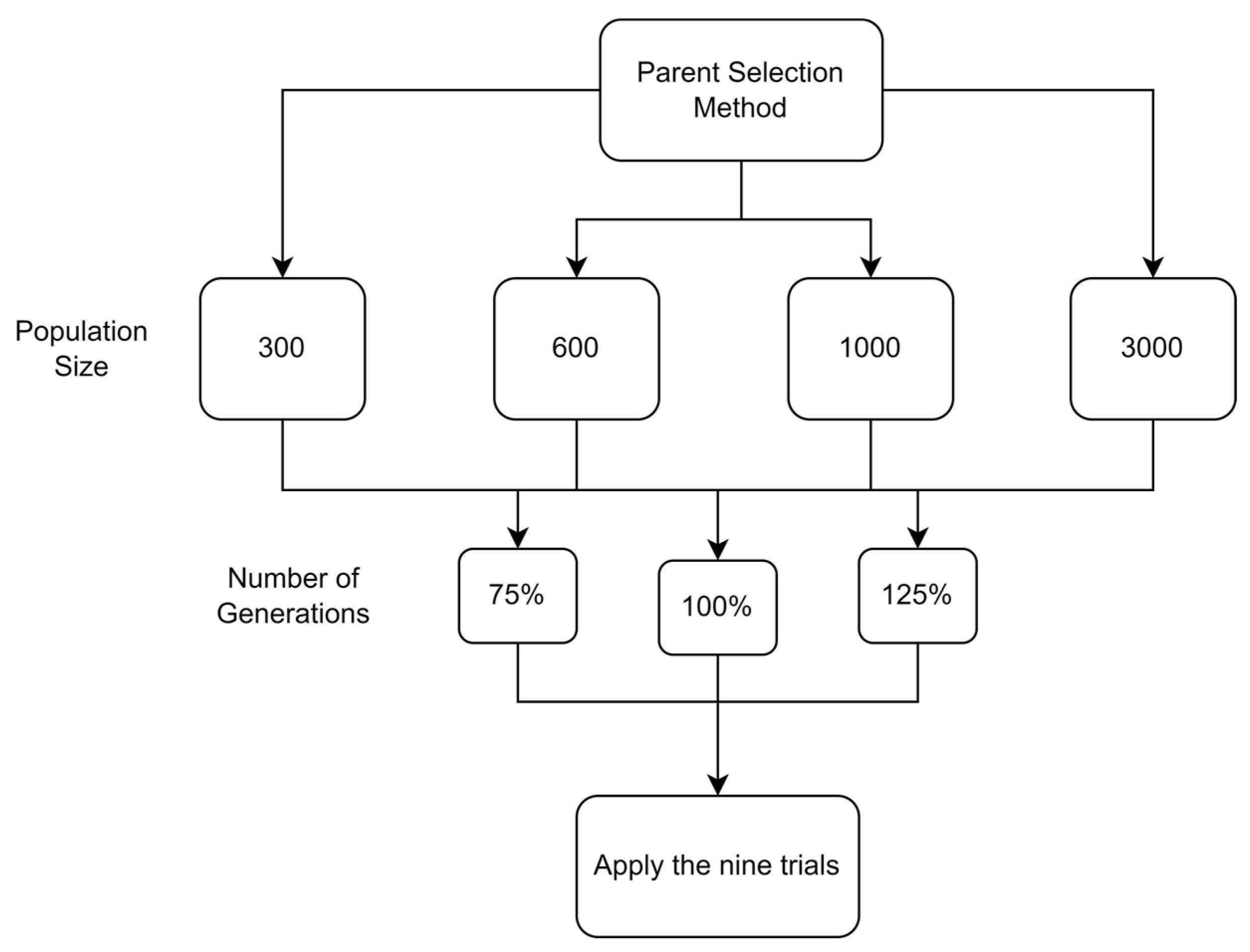
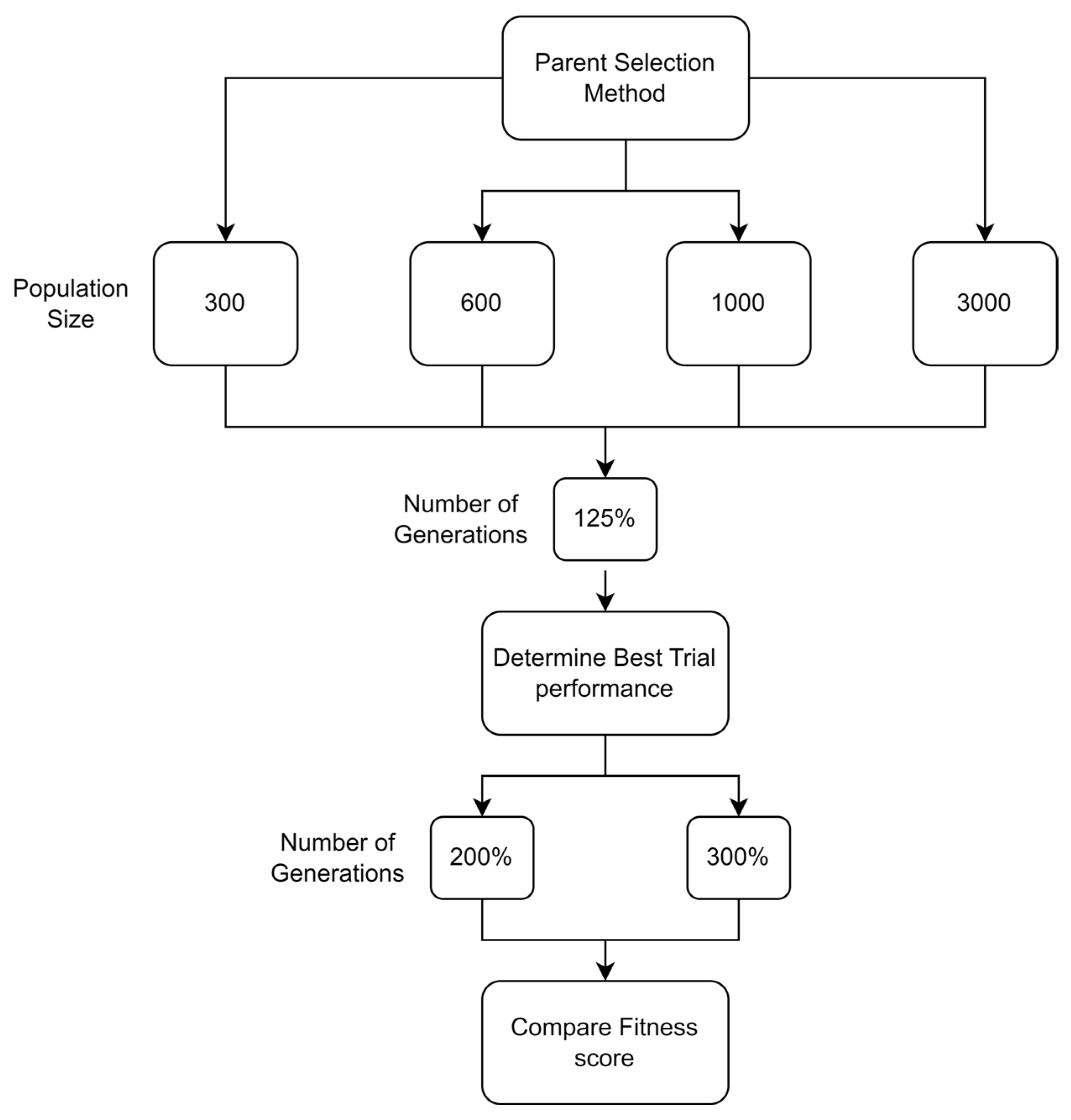

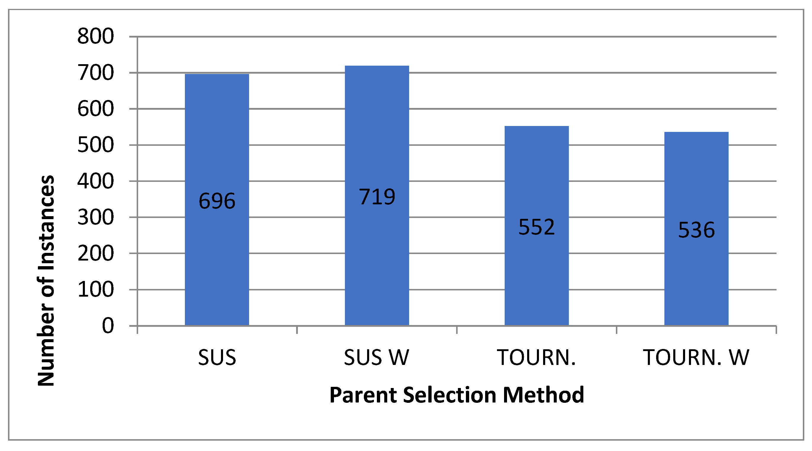
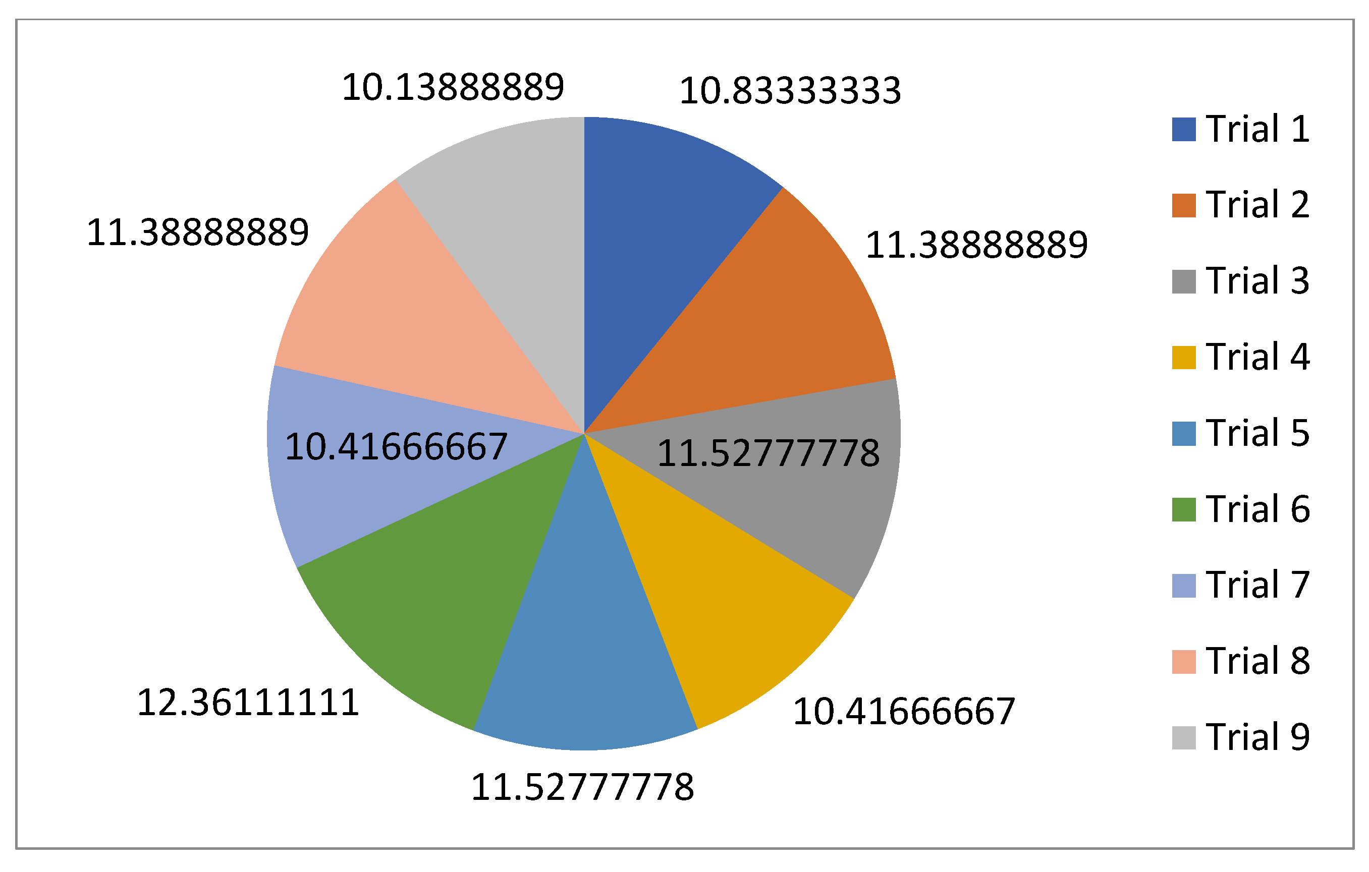
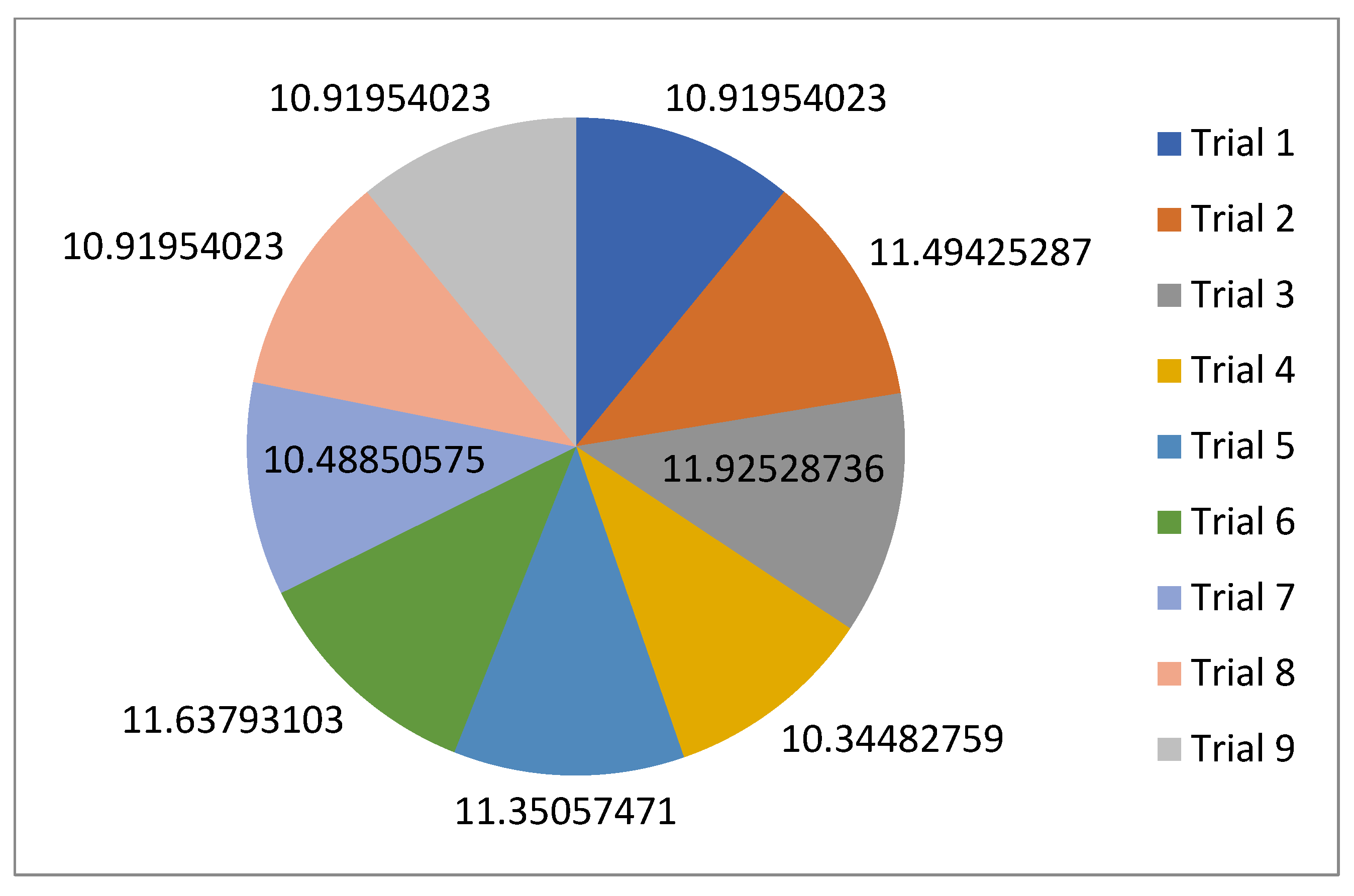
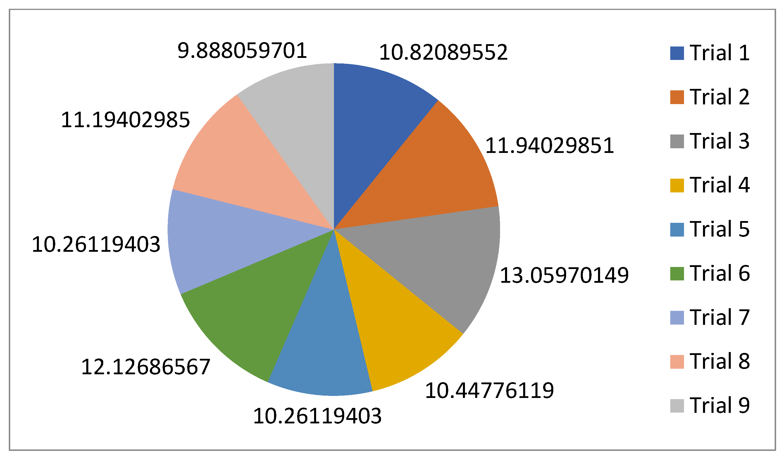
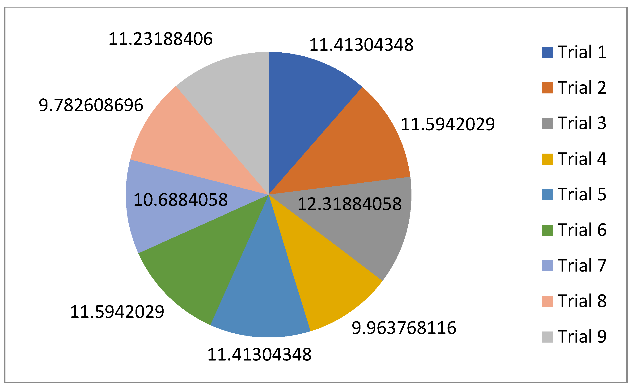

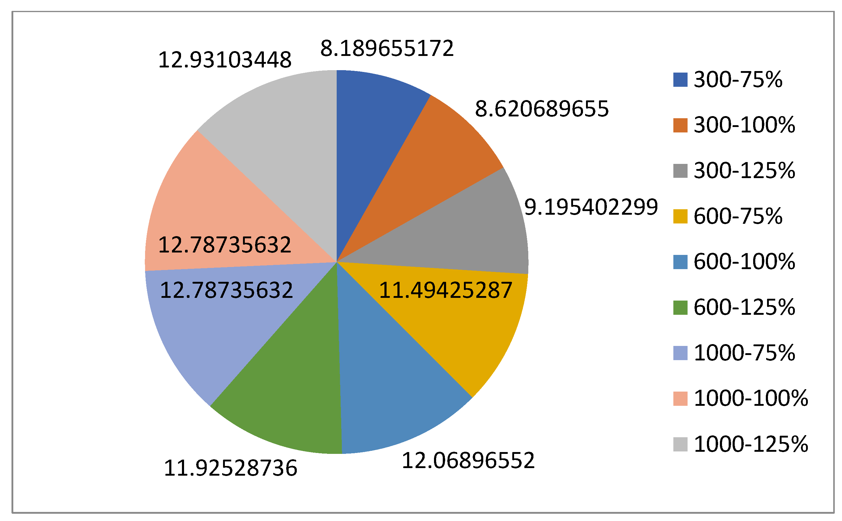


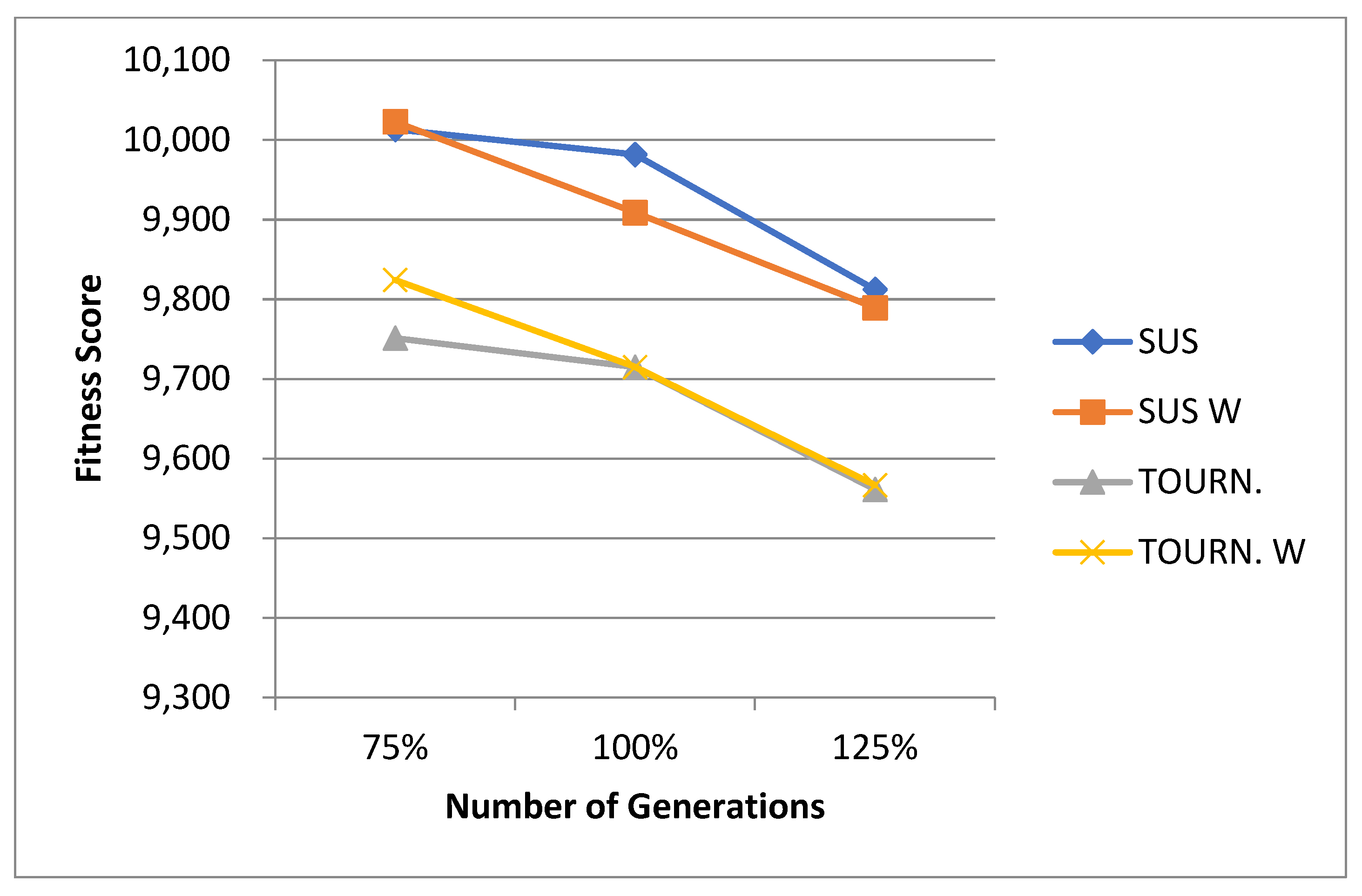
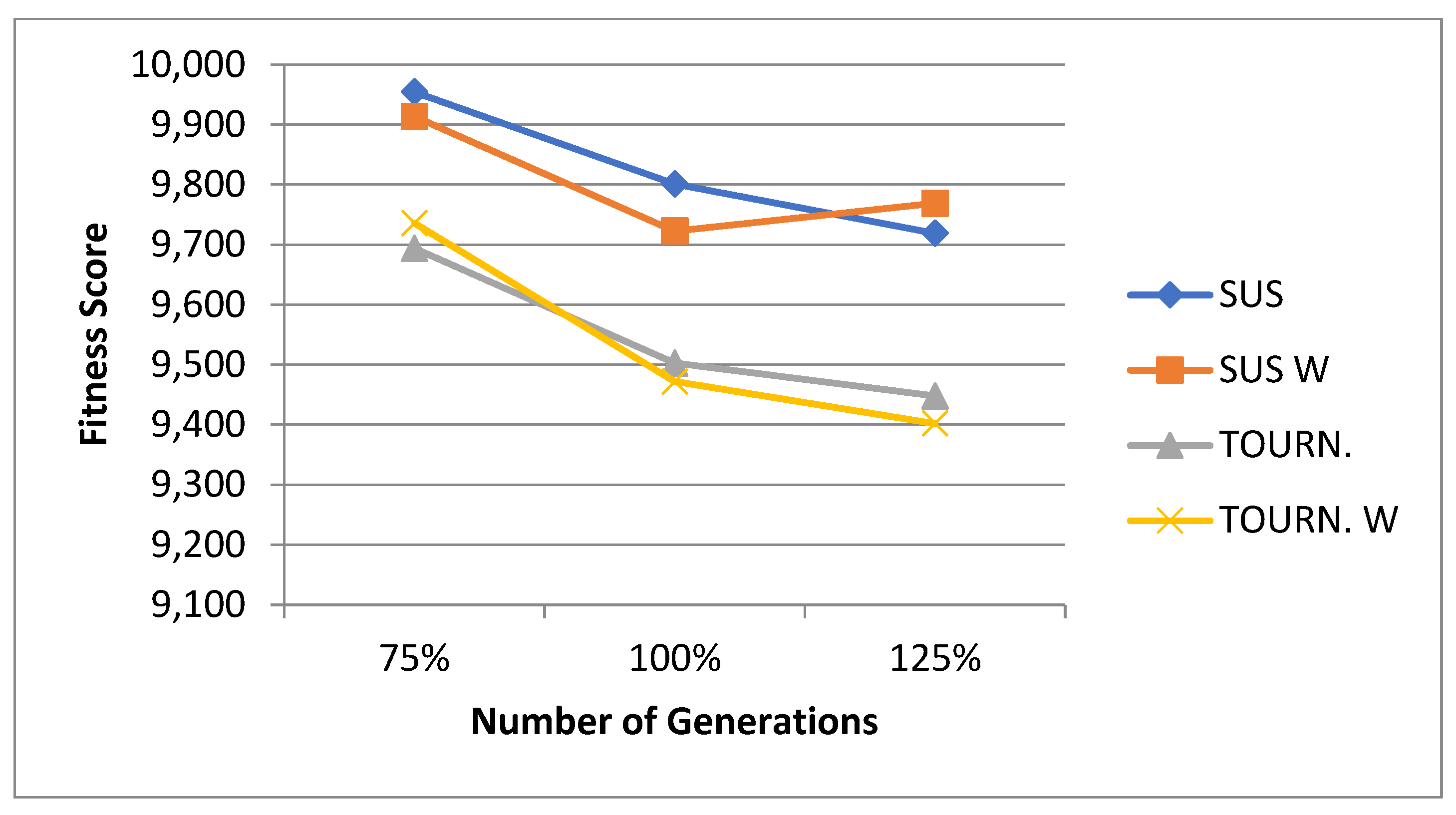
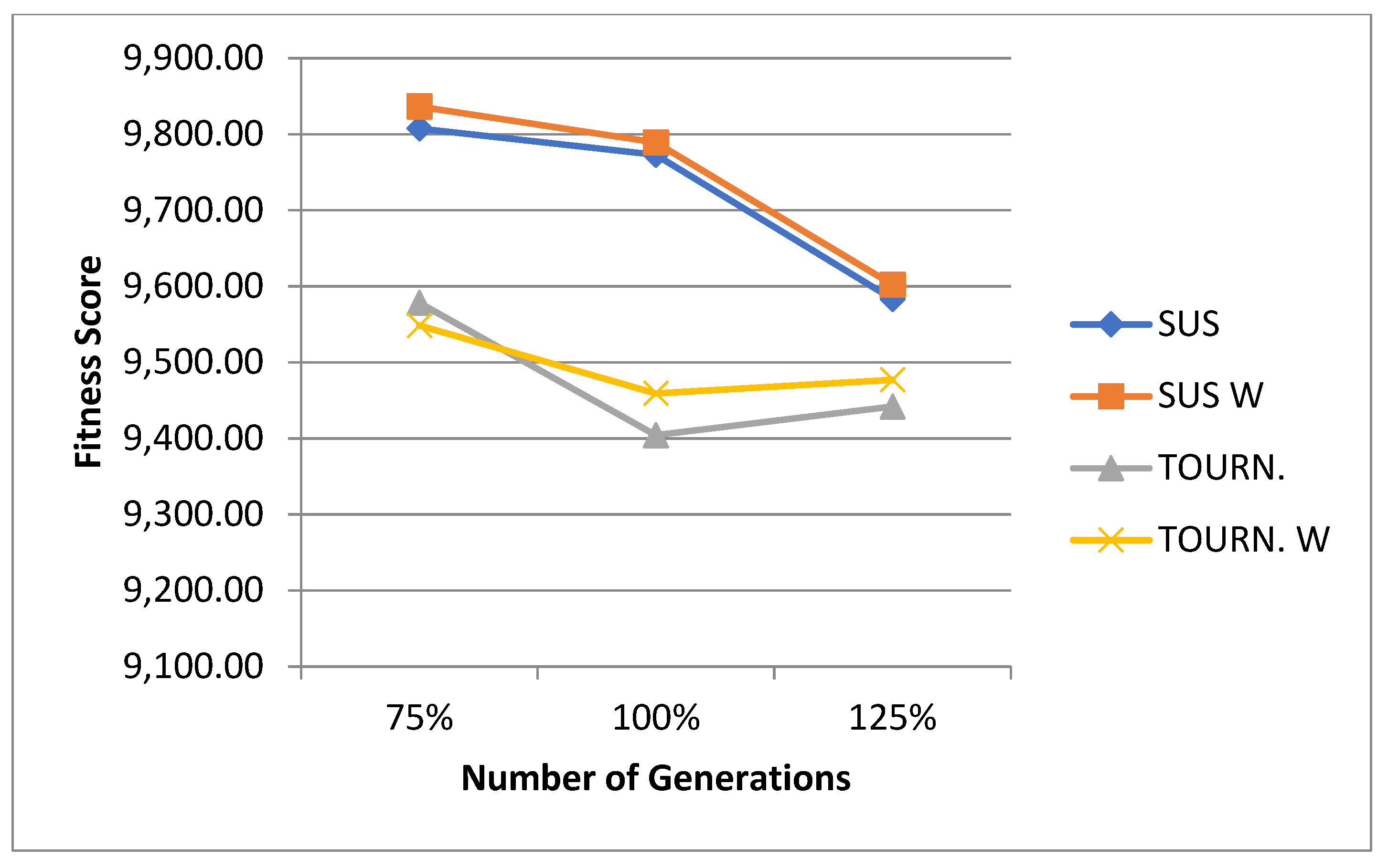
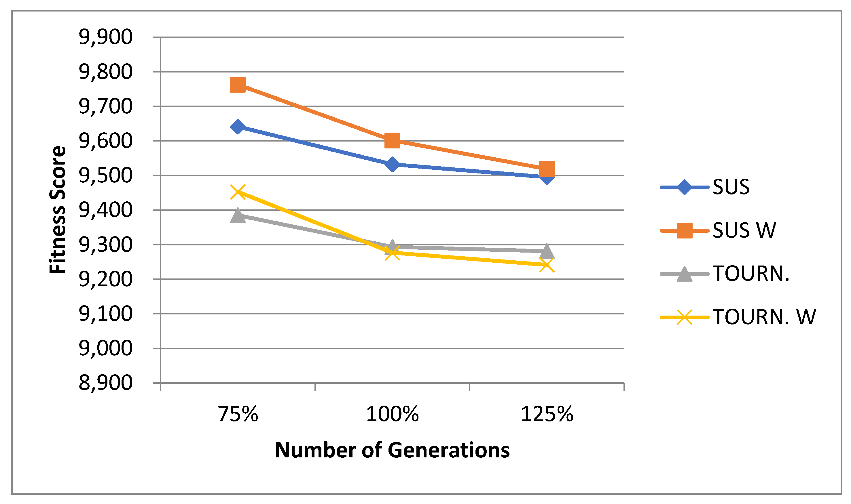
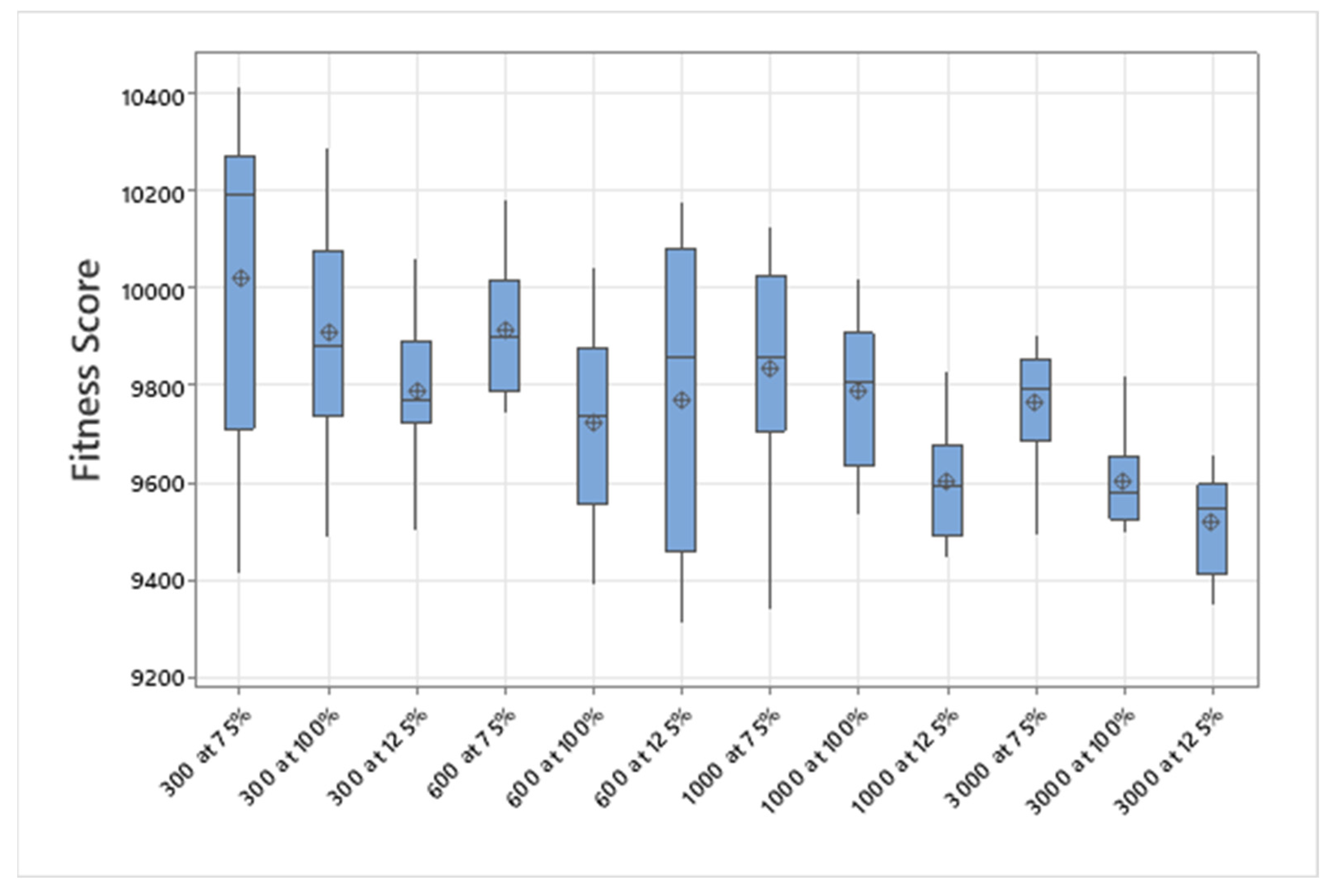
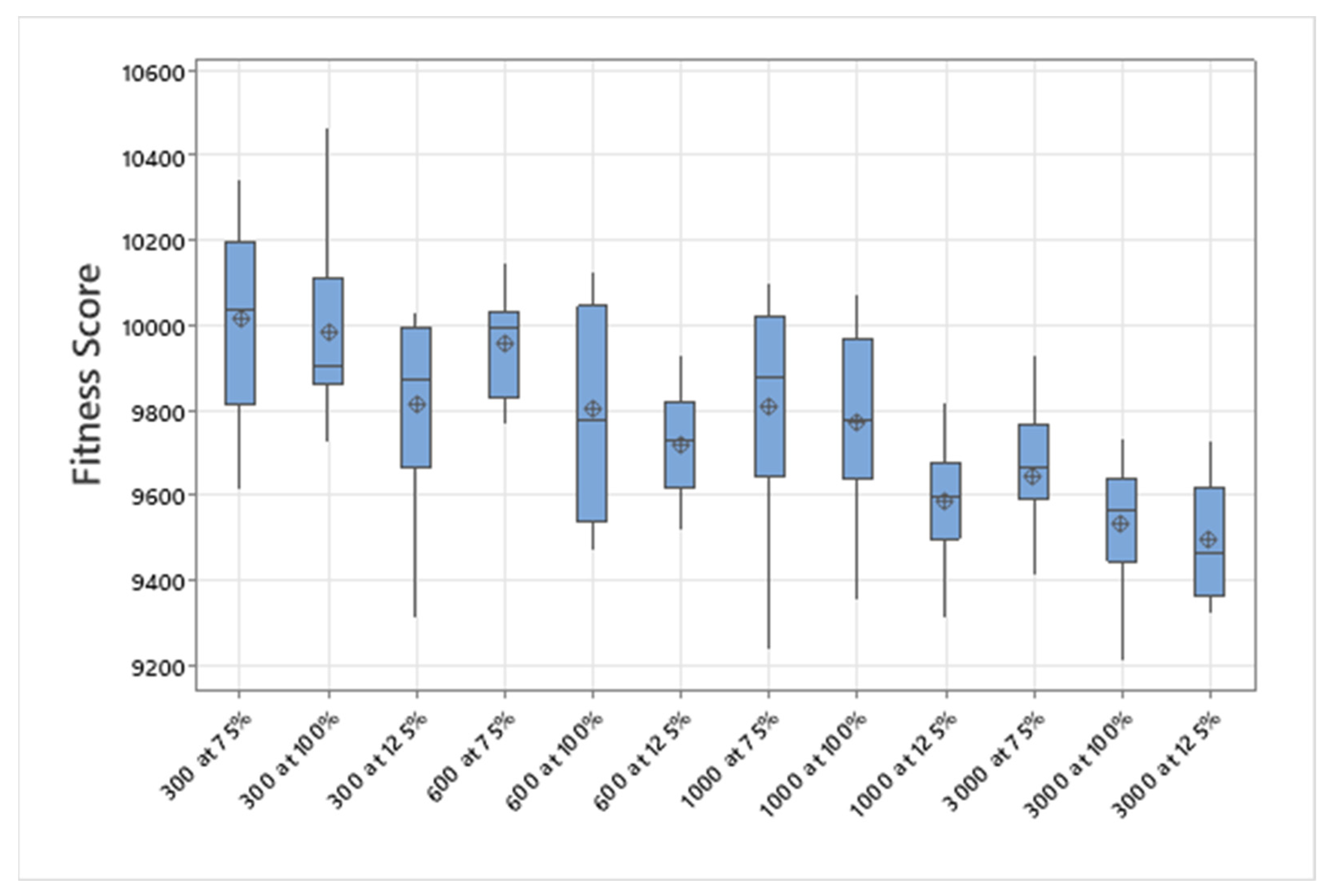


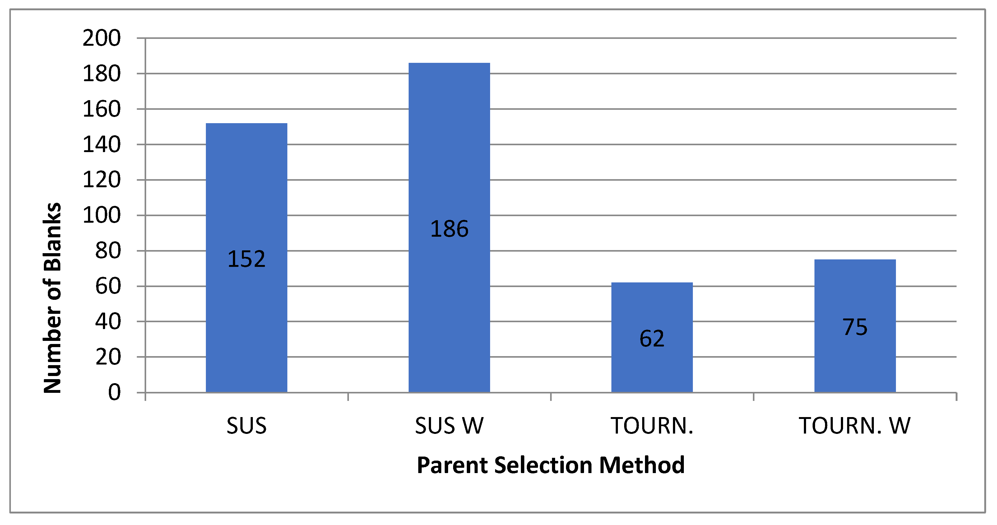

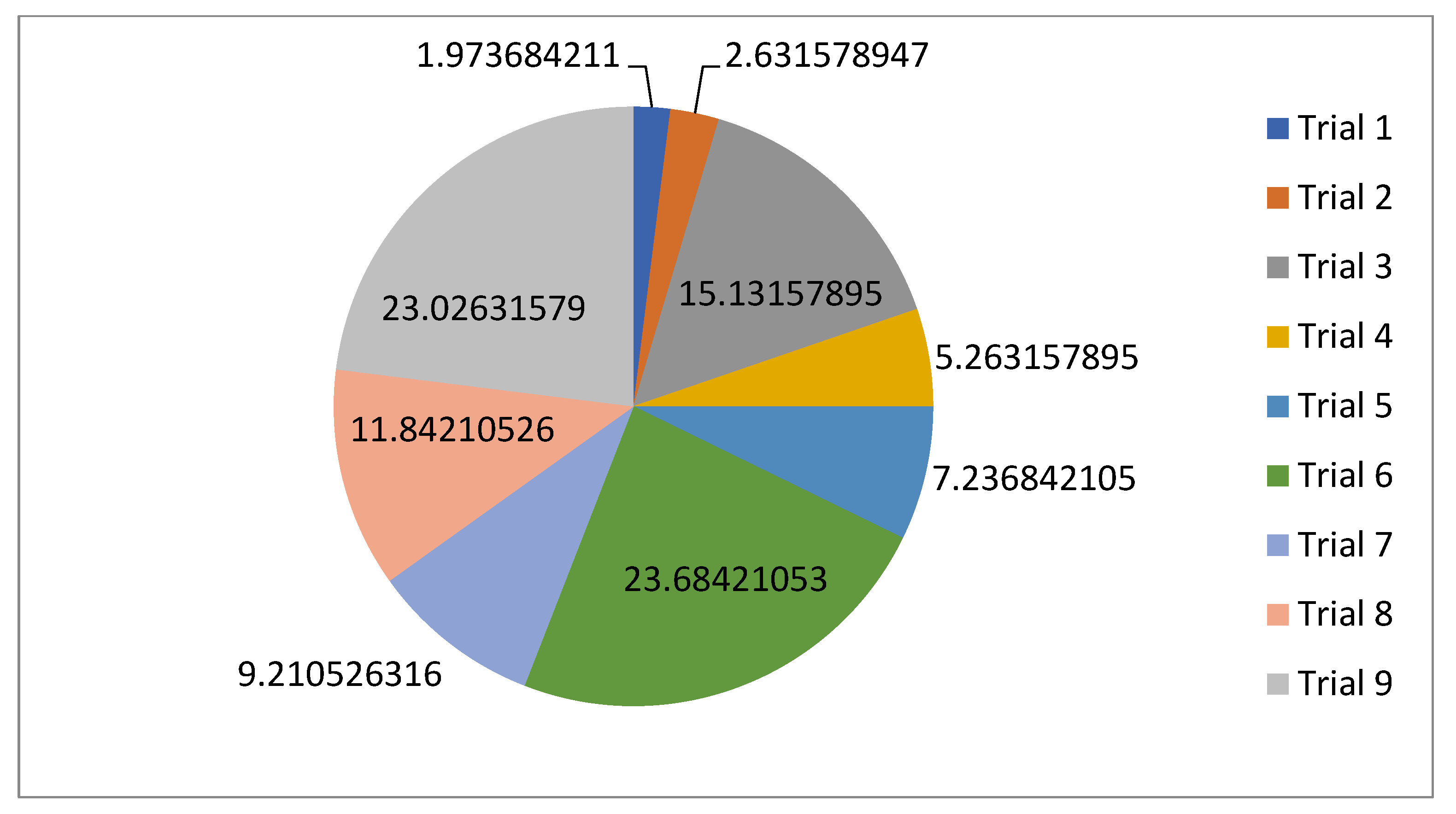
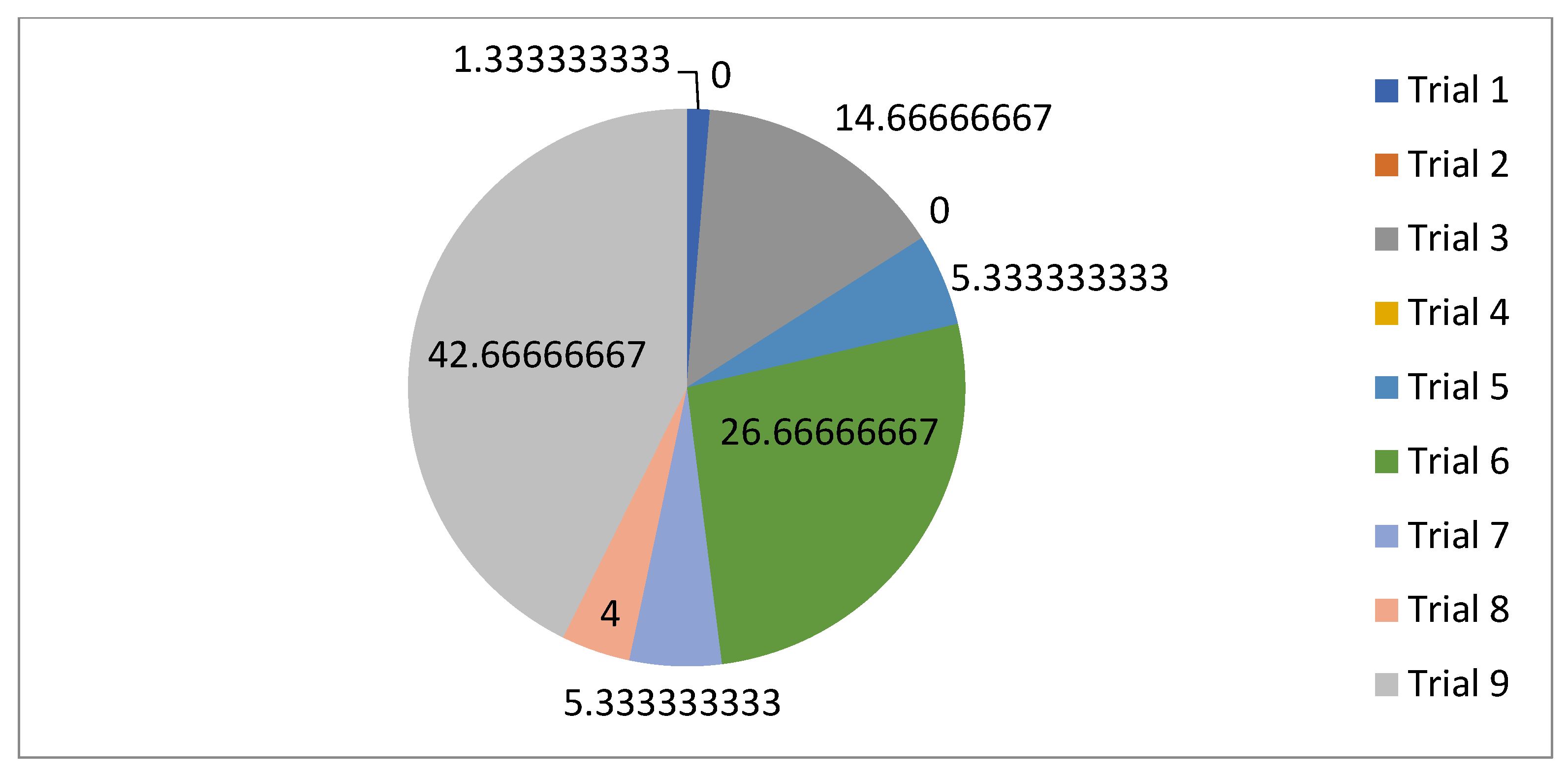
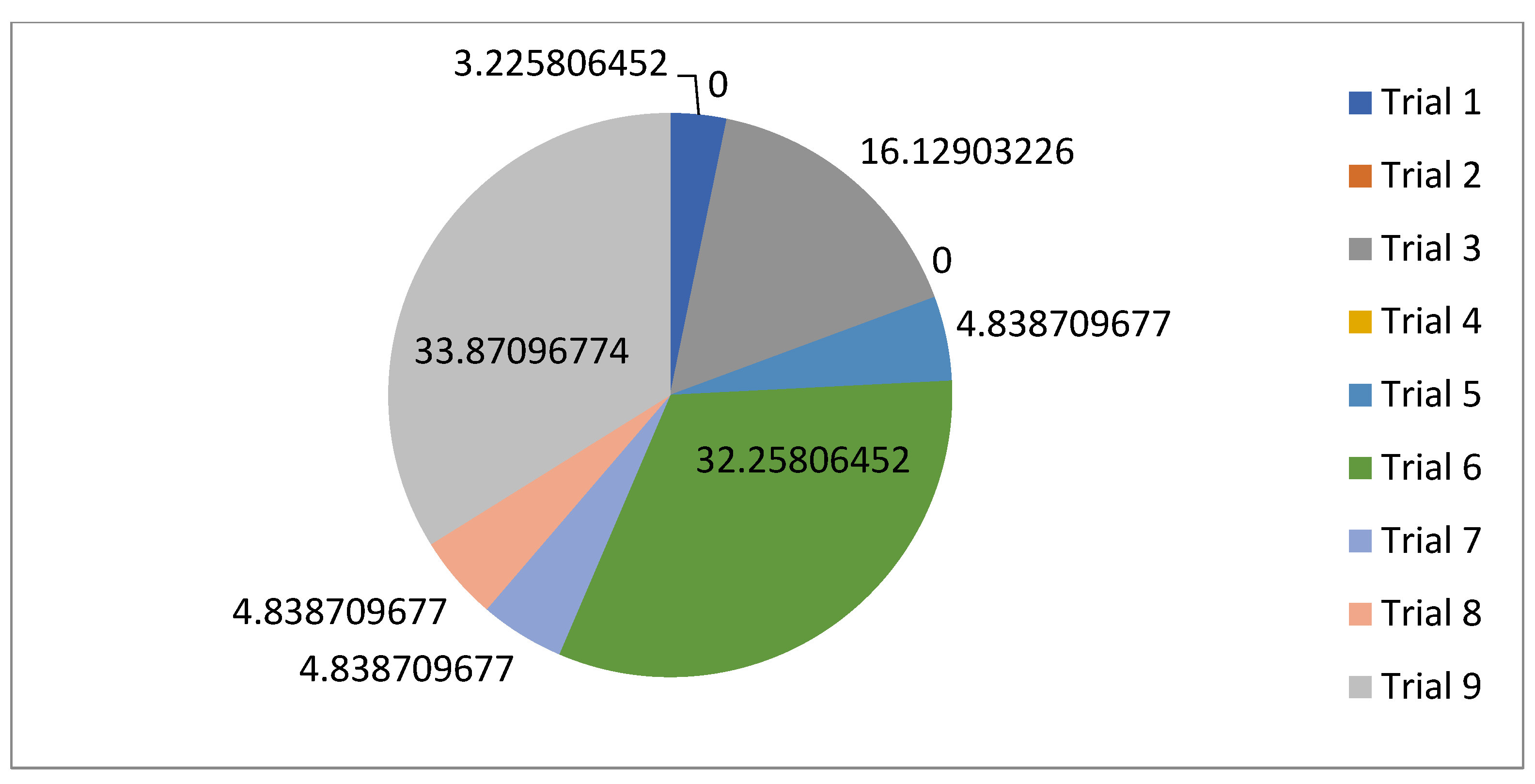
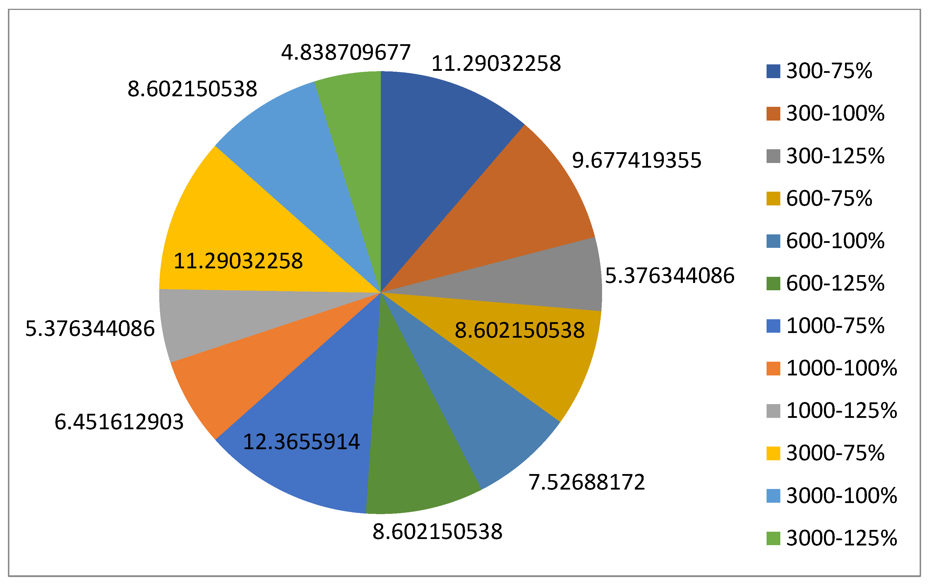
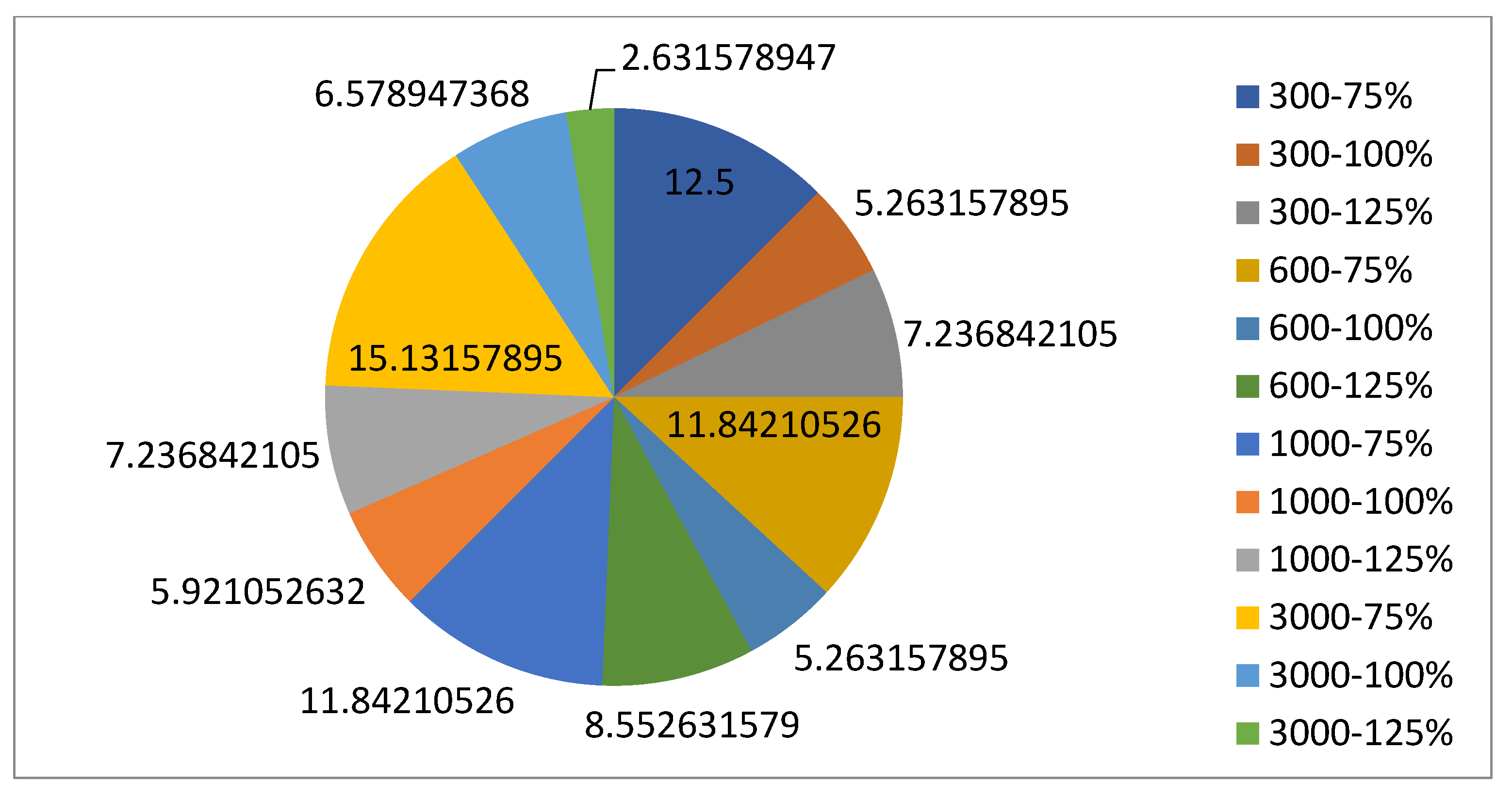
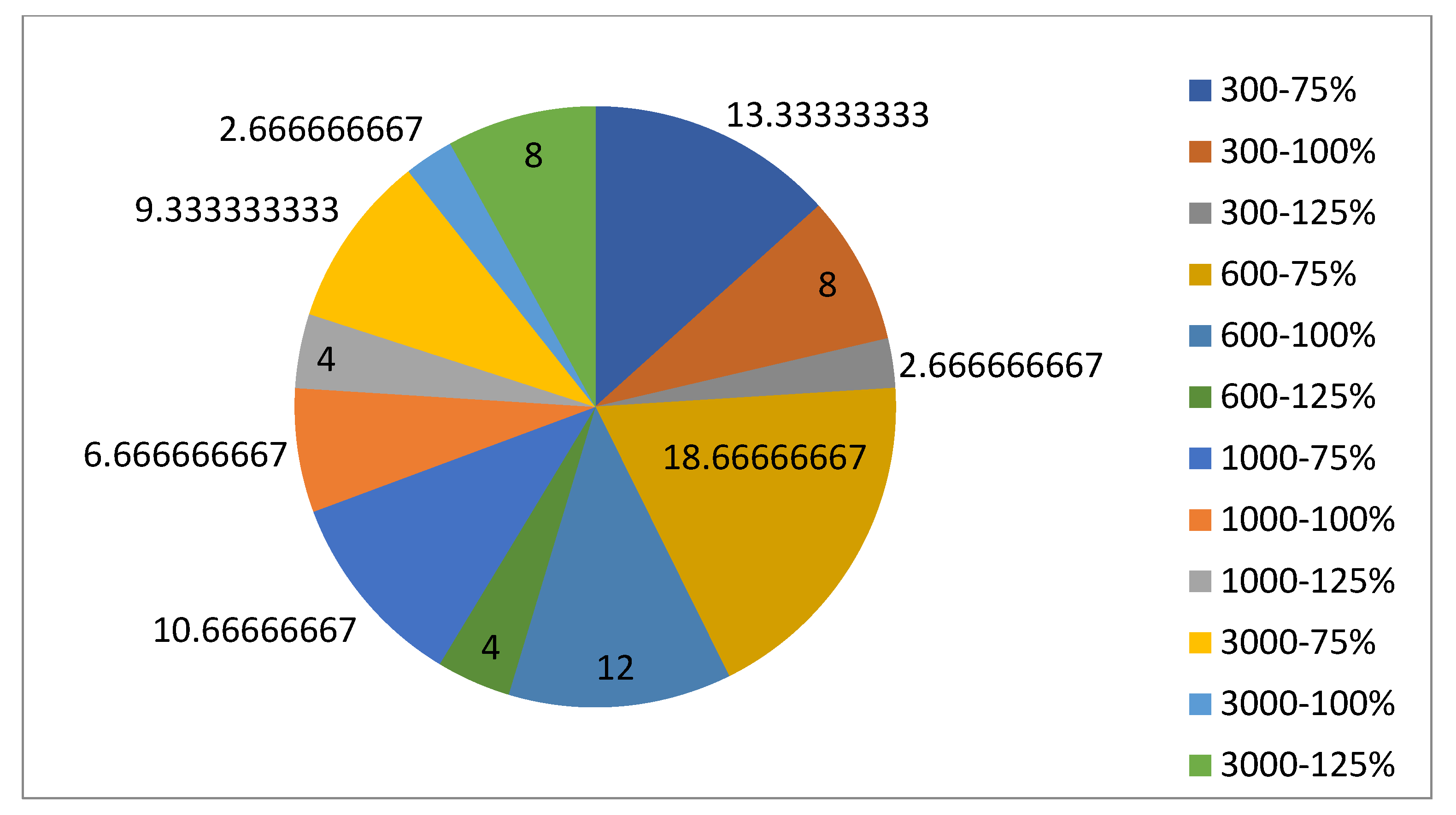
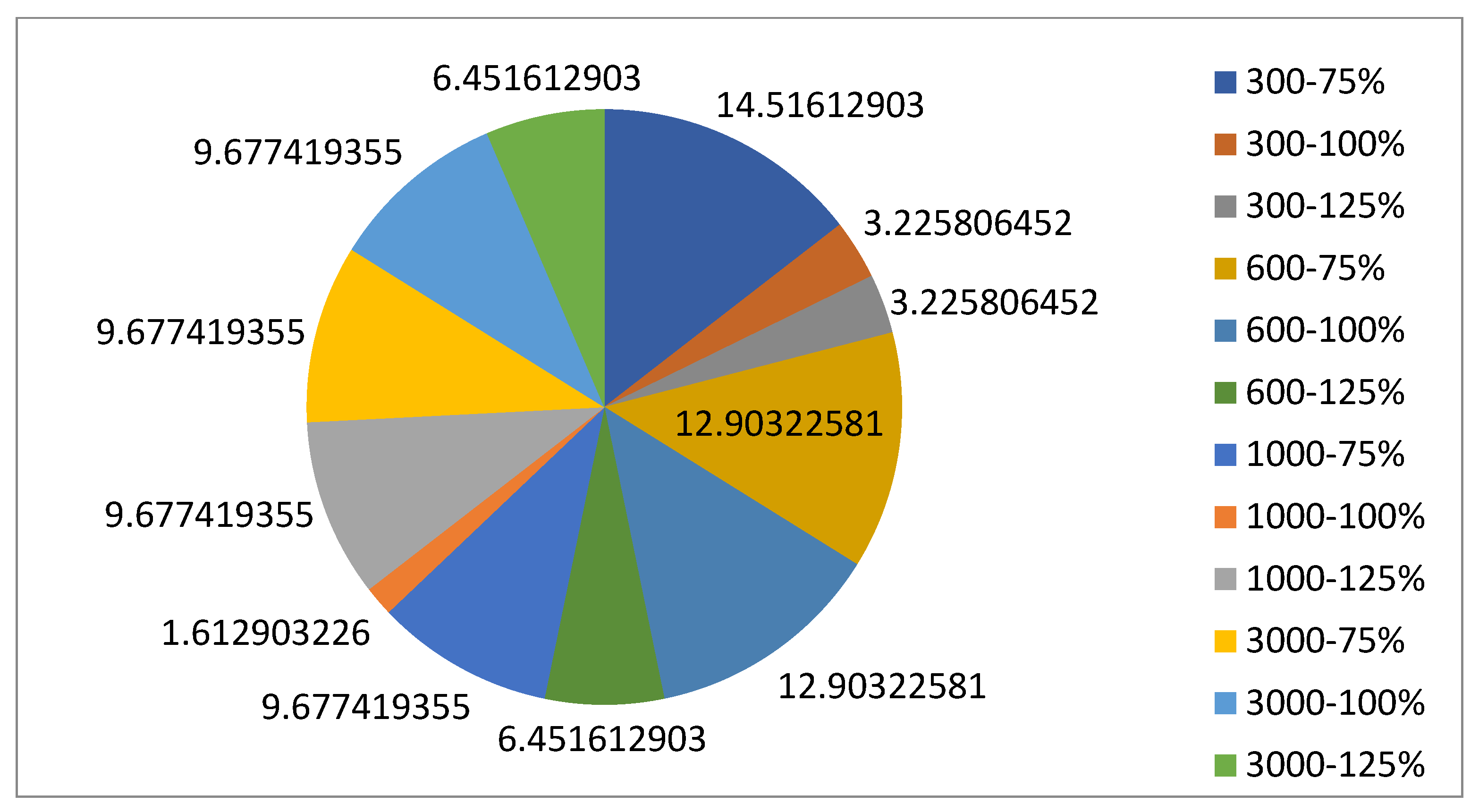
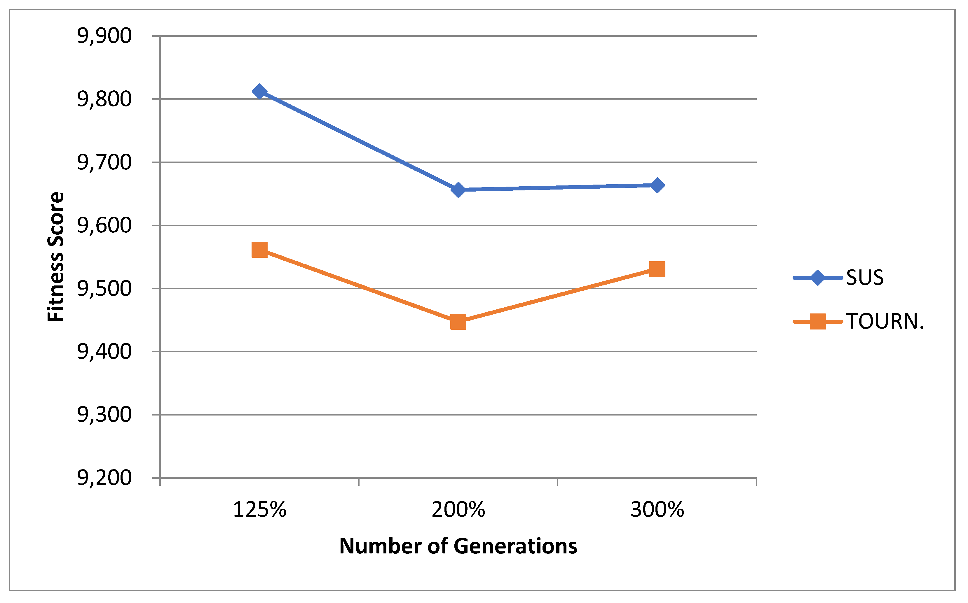
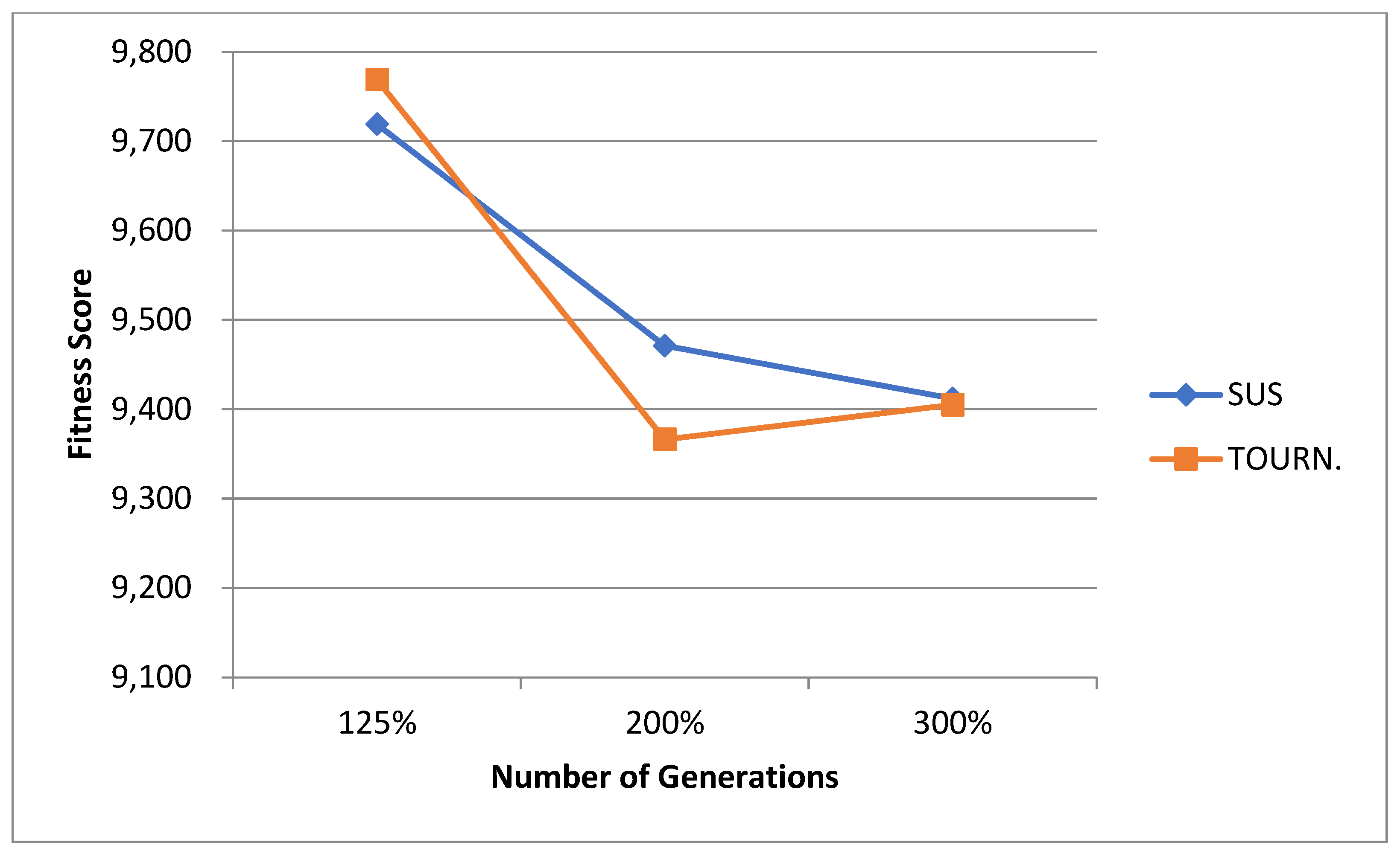
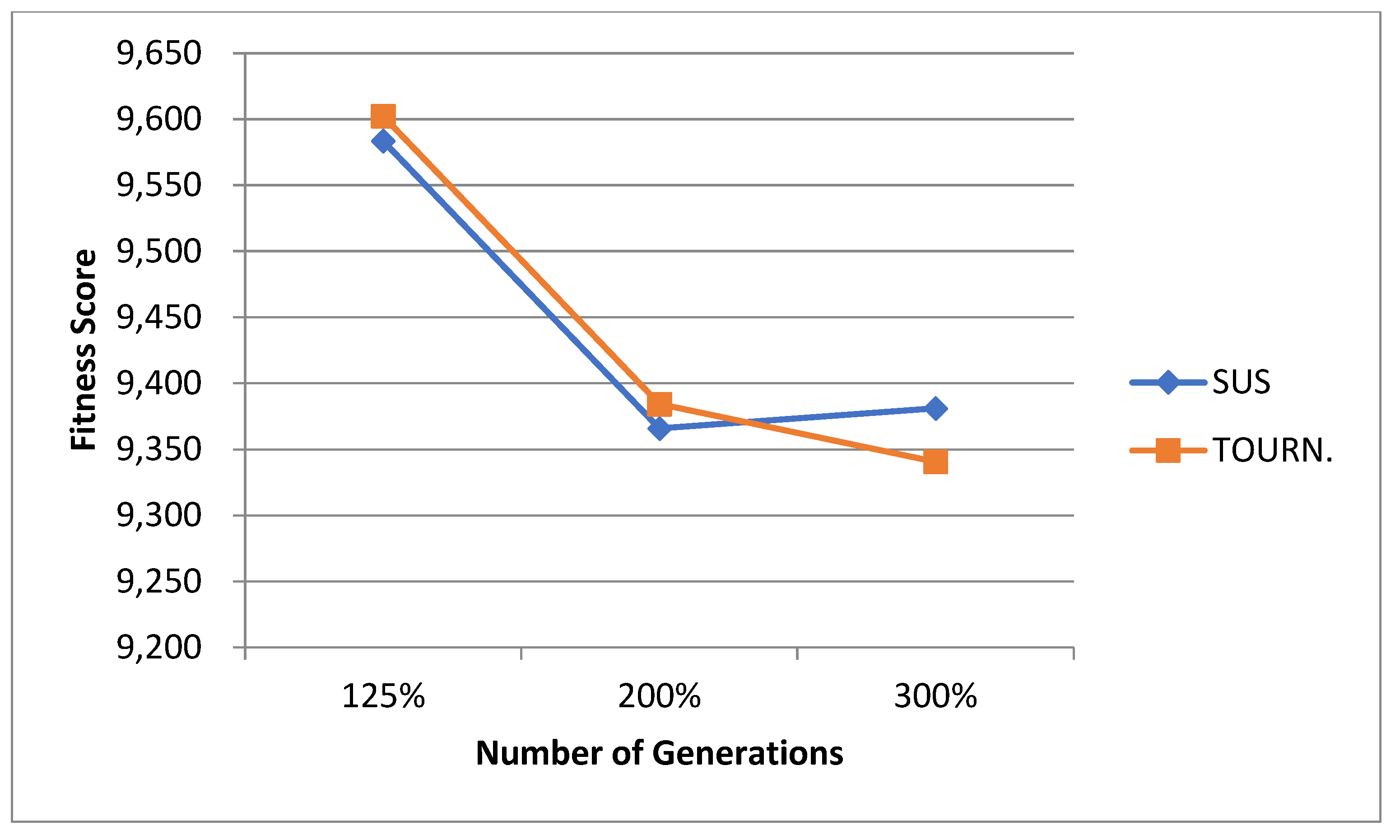
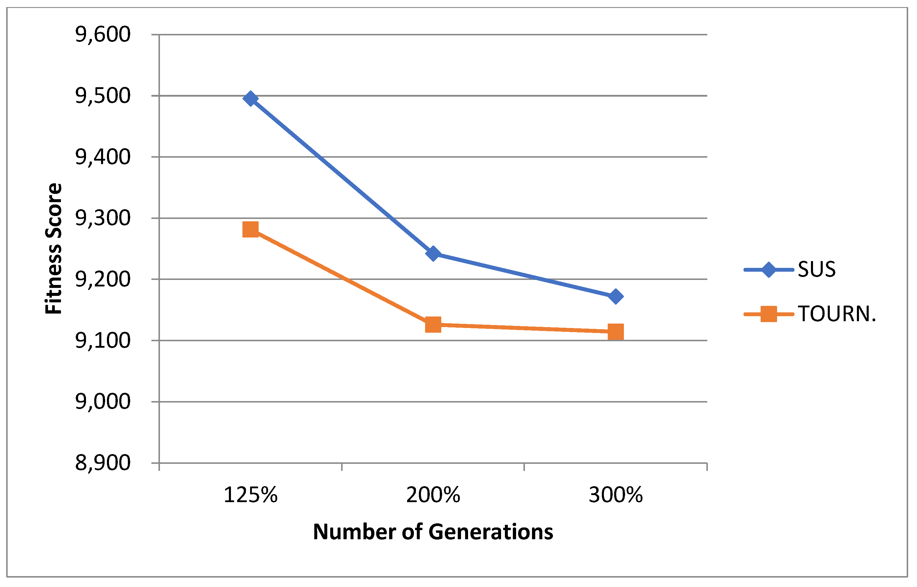
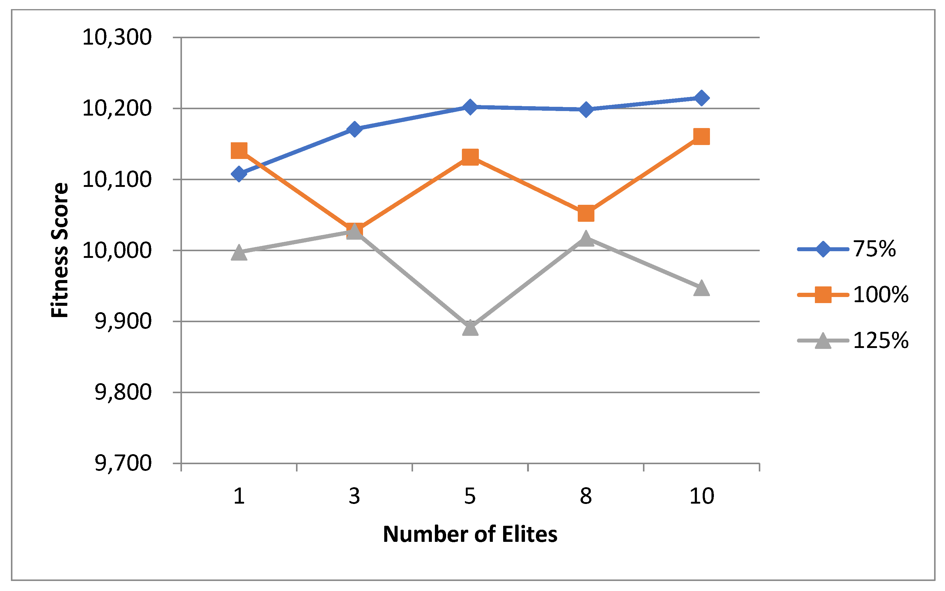
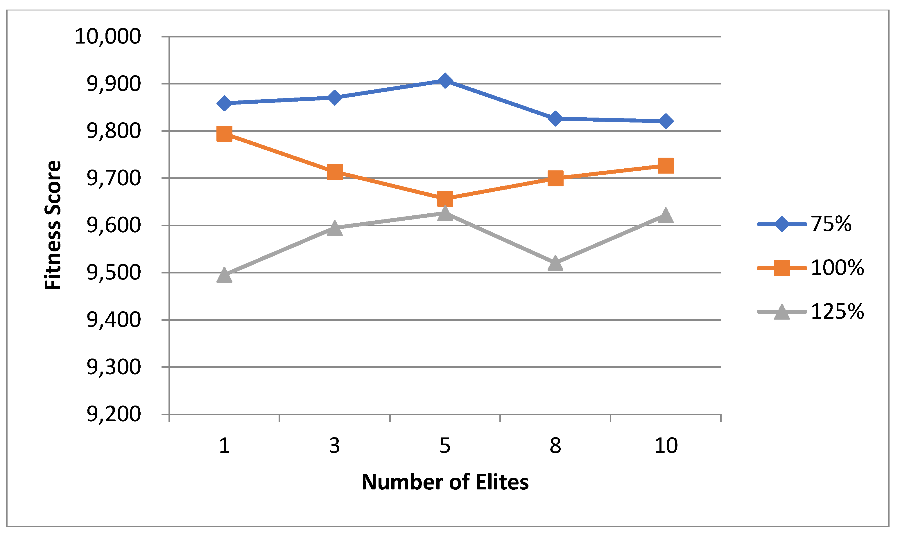
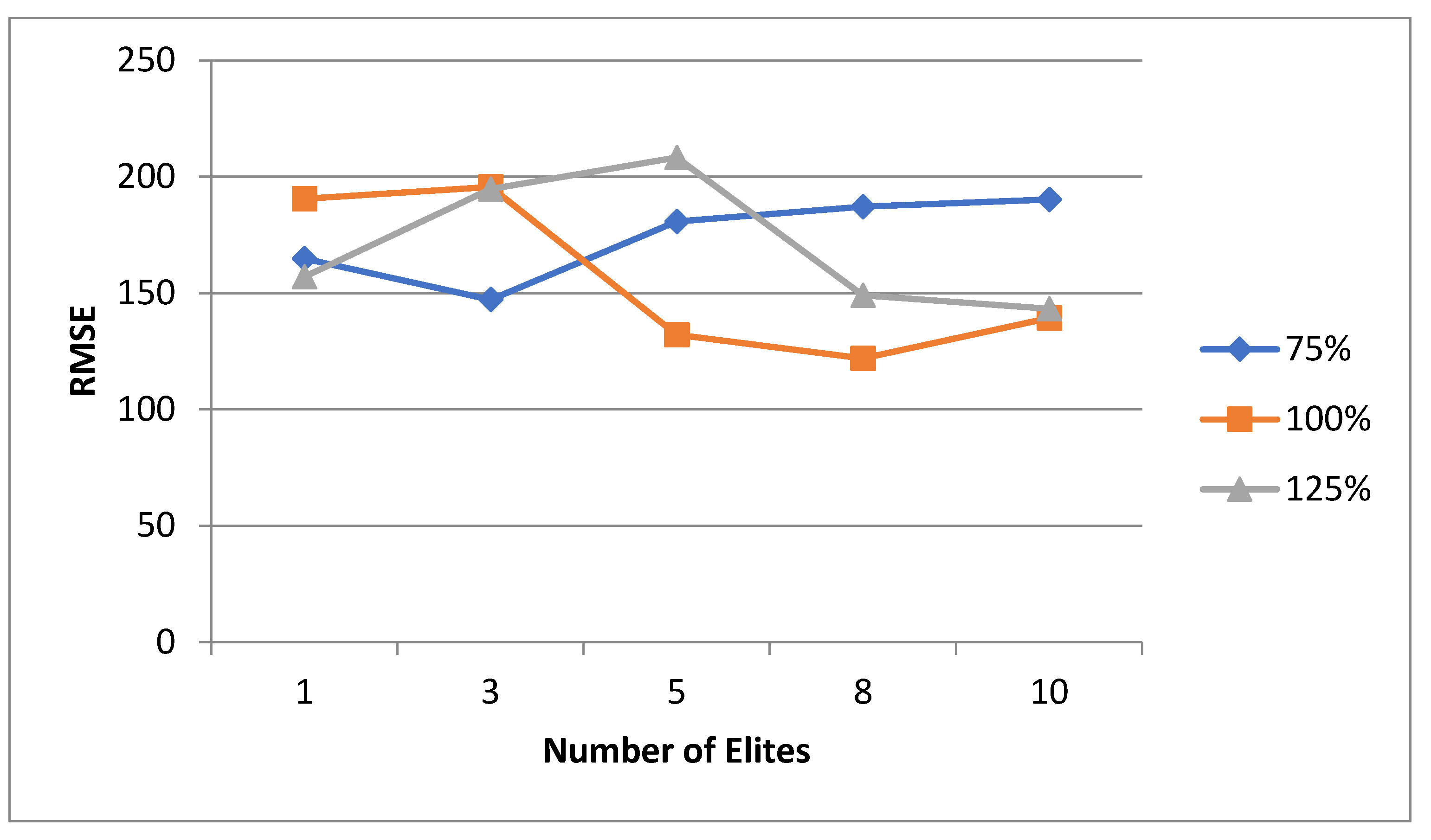
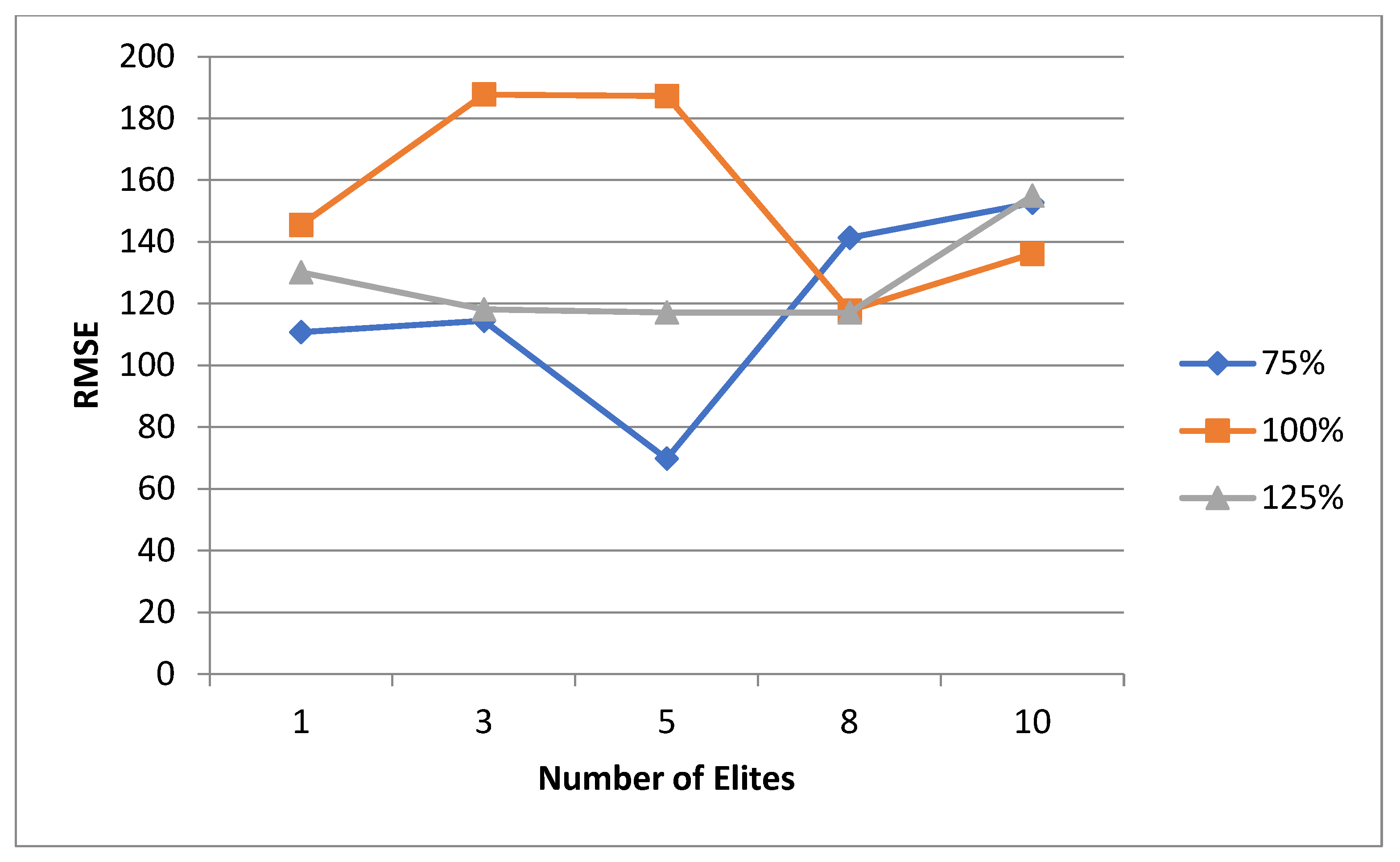
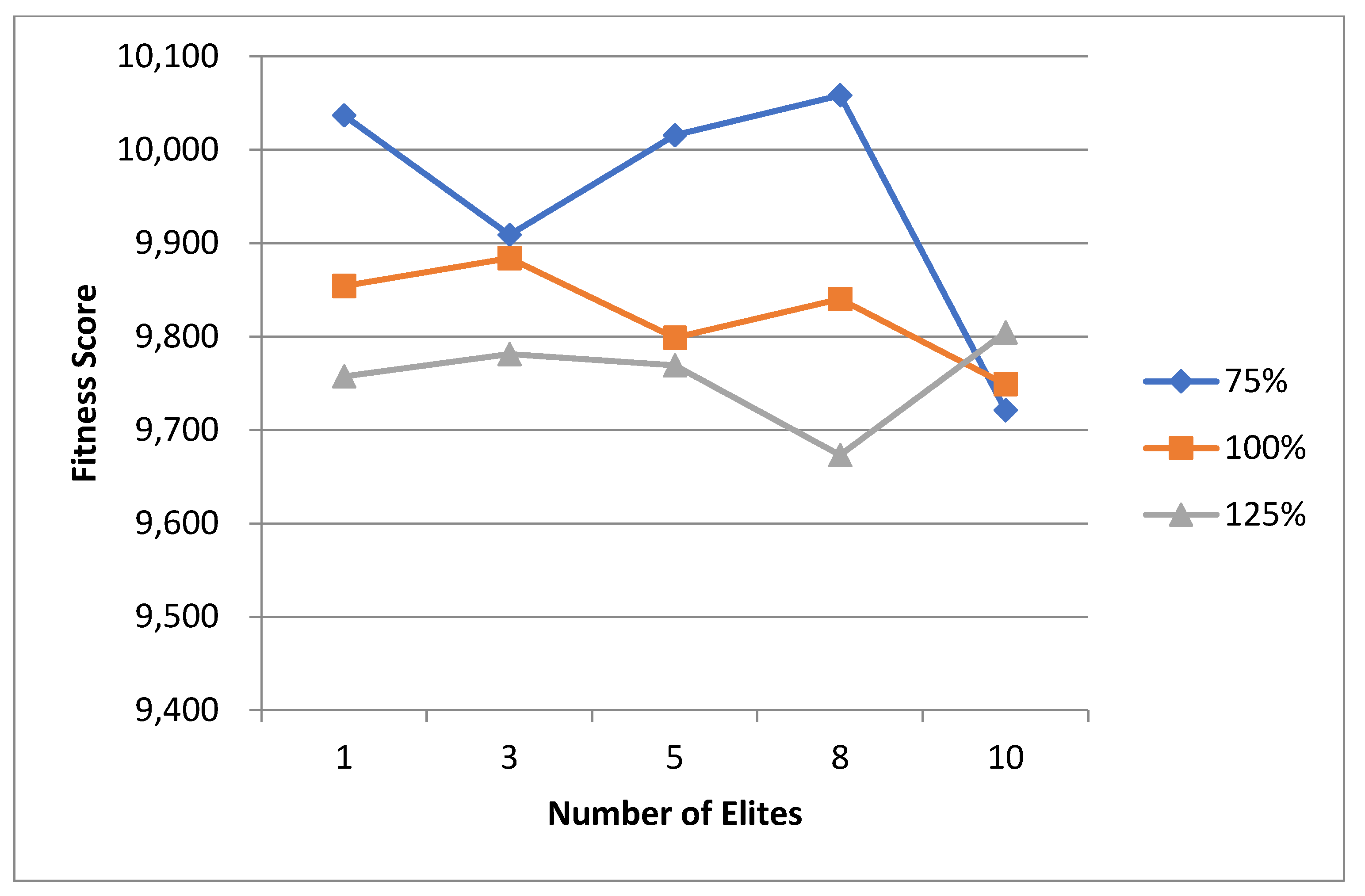
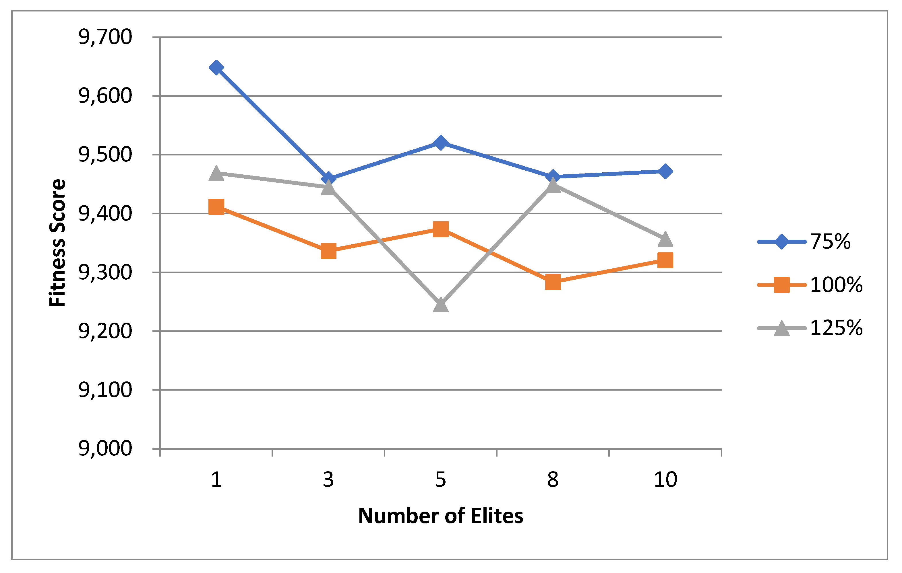
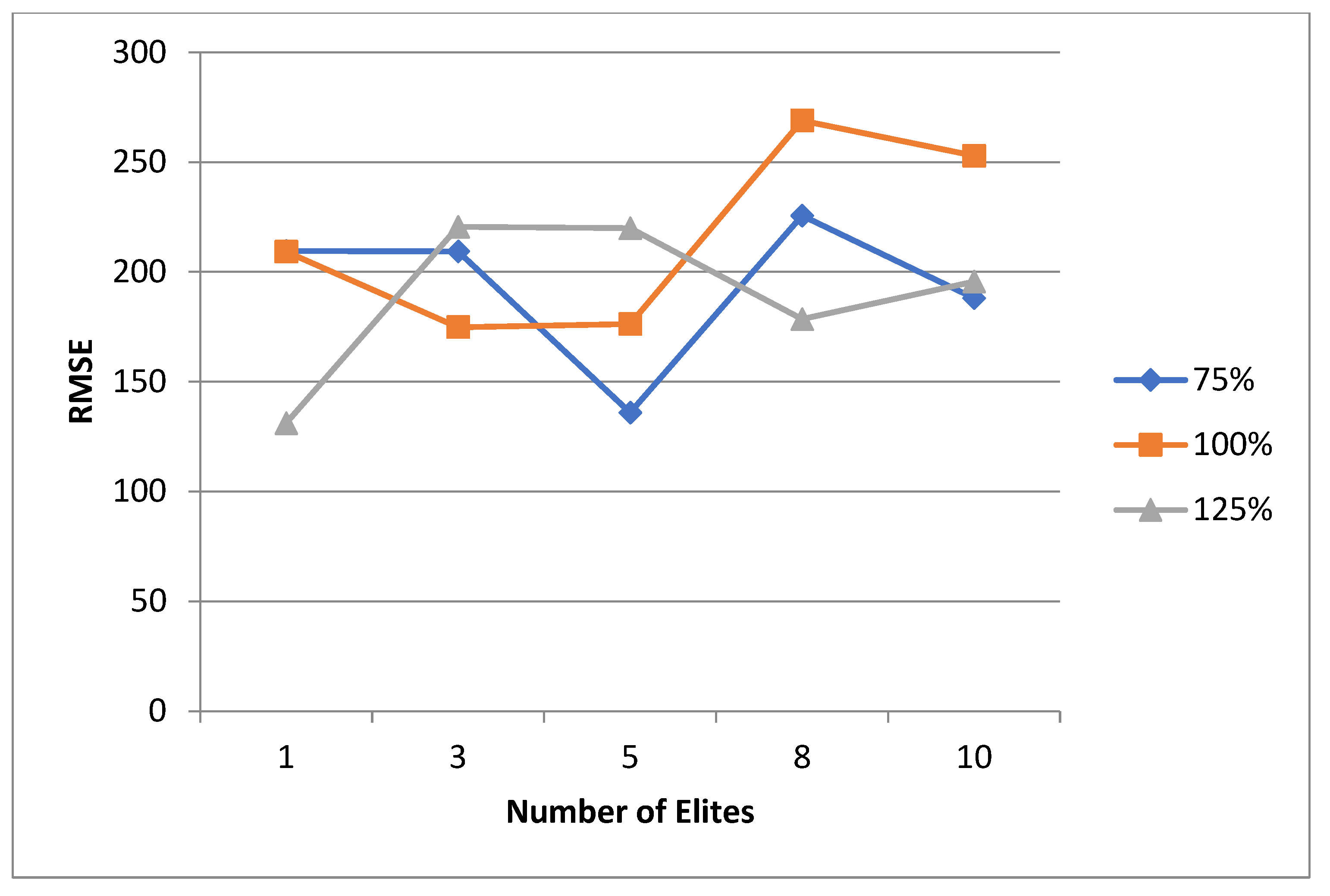

Disclaimer/Publisher’s Note: The statements, opinions and data contained in all publications are solely those of the individual author(s) and contributor(s) and not of MDPI and/or the editor(s). MDPI and/or the editor(s) disclaim responsibility for any injury to people or property resulting from any ideas, methods, instructions or products referred to in the content. |
© 2025 by the authors. Licensee MDPI, Basel, Switzerland. This article is an open access article distributed under the terms and conditions of the Creative Commons Attribution (CC BY) license (https://creativecommons.org/licenses/by/4.0/).