1. Introduction
The condition monitoring and diagnosis of PMSMs are one of the most important and promising directions for the development of effective health index management [
1]. Due to their critical roles as actuators, PMSMs have received widespread applications in important sectors such as advanced manufacturing, energy production [
2], and electric transportation [
3,
4]. Their reliable operation plays a vital role in guaranteeing the efficiency, sustainability, and innovation of these industries, increasing the importance of robust diagnostic and prognostic strategies.
PMSMs face a range of problems like voltage defects, stator and rotor problems, overheating due to voltage problems, and similar issues, which require advanced monitoring and control methods, especially for temperature management. Predicting the thermal behavior of a PMSM is very difficult due to its complexity, which is characterized by nonlinear relationships between mechanical and electrical parameters [
5]. Moreover, temperature significantly affects the efficiency and stability of PMSMs. It mainly causes overheating, one of the most frequent and harmful issues, which occurs because of the pressure caused by the mechanical part of the engine, the core iron, and the copper in the stator windings. Copper losses directly influence heating in the stator windings, leading to the degradation of engine combustion, i.e., the most heat-generating component in it, after which comes an overall system breakdown. Due to this, the engine requires close monitoring and control so that its operation falls within the permissible limit of temperature.
In this regard, the integration of state-of-the-art technologies into the PMSM monitoring framework, such as machine learning models [
6], would be a powerful method for fault prediction and diagnosis and for taking effective mitigations to ensure the general health and uninterruptible operation of the system. Our work investigates how ML-based ANN models could enhance monitoring and prediction capabilities in PMSM temperature control. In this work, four advanced machine learning algorithms are discussed in terms of performance: Convolutional Neural Network (CNN), Long Short-Term Memory (LSTM), Recurrent Neural Network (RNN), and Multilayer Perceptron (MLP).
The key parameters are considered comprehensively by the evaluation methodology: prediction accuracy, computational efficiency, and RMSE are taken into account to enable full understanding of the potential of each parameter in real-time monitoring applications of PMSM. This systematic analysis of the models and pointing out their strengths and limitations are contributory to valuable insights as to how these parameters can be optimized for optimal lifecycle management of PMSMs.
Ultimately, this study contributes to advancing predictive maintenance strategies and ensuring the operational reliability of PMSMs, which are indispensable components in manufacturing, energy production, and electric transportation systems.
2. Related Works
PMSM temperature prediction has been the subject of a considerable number of related studies, which have used a variety of approaches, such as machine learning and hybrid models, to address these issues. A nine-layer deep neural network (DNN) model with a coefficient of determination (R²) of 0.9439 was developed by Zhang et al. [
7] to predict the stator winding temperature. The model demonstrates the effectiveness of deep learning in temperature monitoring systems by significantly outperforming conventional regression techniques. Similarly, Cen et al. [
8] demonstrated the resilience of the approach under various operating conditions and outperformed conventional methods in terms of prediction accuracy by using a long short-term memory (LSTM) network to capture time dependencies in PMSM temperature data.
Chen et al. [
9] proposed a hybrid system incorporating physics-based models and CNNs. Such a combination takes advantage of both physical laws and deep learning methods to make temperature predictions in real time and with high reliability for various operating conditions. Li et al. developed a Back Propagation Neural Network for temperature predictions of the stator and rotor, achieving an excellent correlation coefficient (R
2) between the predicted and actual temperatures. This underlines the importance of temperature monitoring, which allows maximum performance for PMSM and prevents overheating. Furthermore, Li et al. [
10] proposed a hybrid model that combines neural networks with LPTN to give better temperature predictions in multiple nodes, especially under conditions of limited training data. LSTMs have been used to correct uncertainties and faults in the physical model, whereas LPTNs compartmentalize complex thermal interactions into a network of nodes and thermal resistances. Liu et al. [
11] have also developed a method that combines machine learning and physical modeling, using the outputs of the physical model as inputs to a neural network. This method shows the effectiveness of real-time predictions by incorporating sensor data in the physical domain through data-driven methodologies.
Hence, the combined findings of these investigations mark a substantial step forward into the realm of PMSM temperature supervision and monitoring, suggesting that ML frameworks, including those using AI reinforcement learning, hold the potential of being very strong tools for better system safety and reliability.
3. Methodologies
This section presents the methodologies employed in this research. It begins with an overview of the prediction process based on the ANN inference model, followed by a detailed explanation of the functioning of each machine learning model among the four predefined algorithms. Finally, it introduces the performance indicators used to evaluate the results of each model.
3.1. ANN-Based PMSM Temperature Prediction Process
The temperature prediction of PMSMs using ANNs requires the preparation of this dataset, which was initially stored in a CSV file. Multiple preprocessing steps were performed to provide ready high-quality data and prepare this dataset for training our ML models (
Figure 1). The first step is normalization, which will scale all the input variables within a common range. This step will eliminate the existence of value differences between features. This step improves model performance by preventing large variables from dominating. Next comes the cleaning stage, which is performed to remove any inconsistencies, outliers, or irrelevant data, so that only correct and relevant information is fed into the model.
After cleaning, imputation addresses missing values by replacing them with appropriate estimates, preventing data gaps from affecting the learning process.
After the preprocessing is performed on the data, it is standardized, resulting in a dataset with similar qualities. The standardized dataset is then divided into a training and testing set, usually an 80%/20% split. The training subset is for training the ANN models, and the test set is used to evaluate the models’ performance and generalization capacity.
The data, once prepared, are then fed into the predictive model inference layer of the ANN framework. We separately implement and train four ANN models (MLP, RNN, LSTM, and CNN) for the temperature prediction of PMSM. Each model produces its temperature outputs, which are later subjected to three measures: the root mean square error (RMSE), the mean absolute error (MAE), and the coefficient of determination (R2) of all models. These metrics encapsulate the accuracy, repeatability, and confidence of each model described. Ultimately, the performance evaluation determines which model will be used in the next stage for the reliable and efficient prediction of PMSM temperatures.
3.2. ANN-Based Machine Learning Models
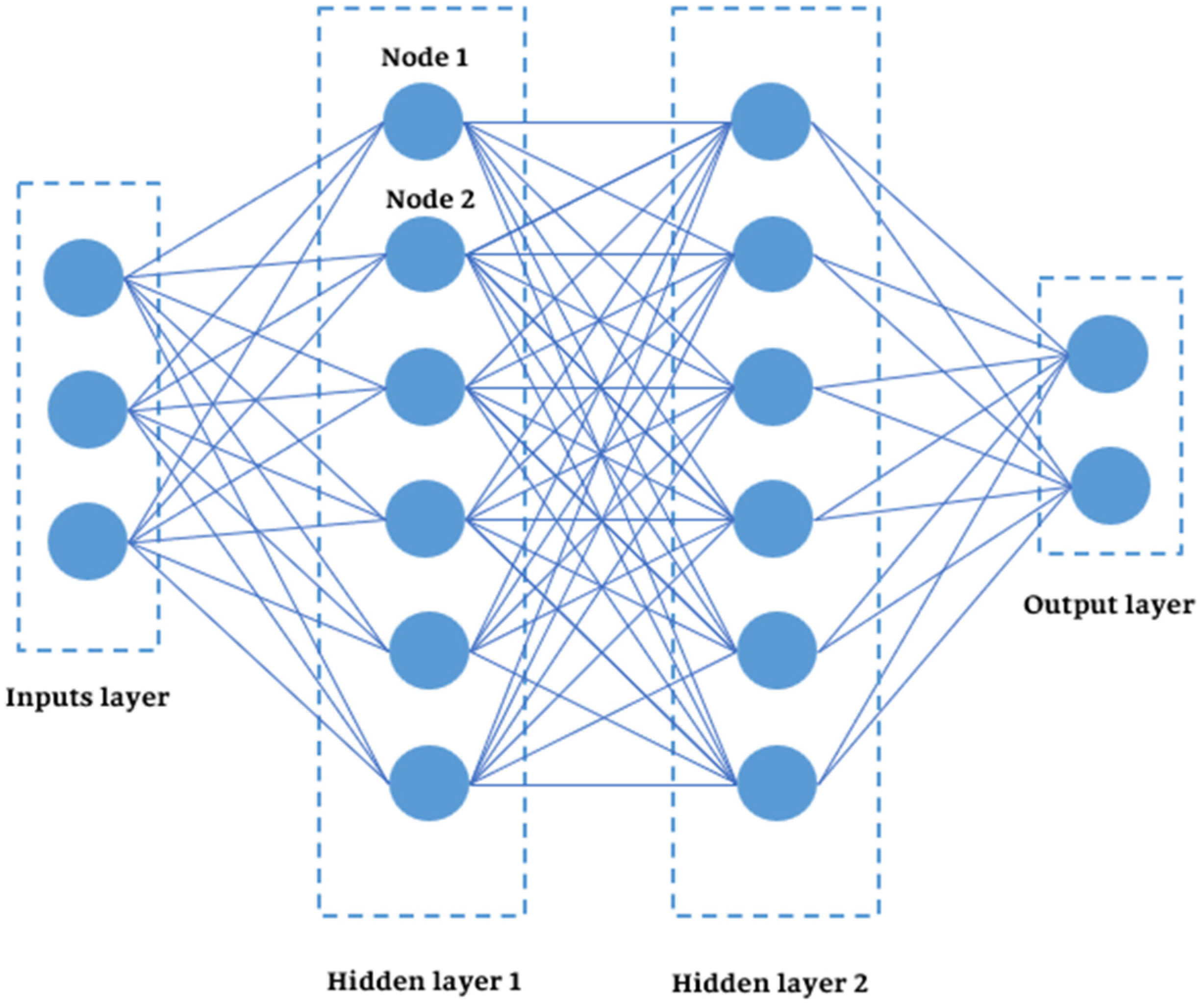
3.2.1. Multilayer Perceptron (MLP)
The MLP is a versatile machine learning model suitable for a wide range of predictive tasks [
12]. It receives a set of input variables that characterize the system being studied. The model’s capacity to accurately identify essential associations in the data can be enhanced by thoroughly preprocessing and normalizing these input variables [
13]. MLP is an inclusive family of models. The input layer is in charge of collecting the input variables passed to one or more hidden layers [
14,
15]. The standard architecture and design of these hidden layers are fundamental for the general performance of the model; there are many tuning parameters that may strongly influence the capability of the model to carry out tasks with high accuracy in a time-efficient way [
16]. Thus, a weighted sum over the ingested input, followed by the ReLU-Rectified Linear Unit, Sigmoid, and GELU, among others, as activation functions introducing nonlinearity in the following steps, would enable the modeling of intricate patterns and relationships through back propagation, which is crucially embedded into these kinds of hidden layers of results [
17]. Eventually, the hidden layer results in a combination that will present their output over an output layer. This acts in the development of the eventual prediction or classification.
A typical MLP model, as shown in
Figure 2, consists of an input layer containing
m input variables, one or more hidden layers with a number of nodes, and an output layer corresponding to the prediction target [
18]. This flexible shape allows the MLP to model a wide range of functional forms (regression, as well as classification, and more specialized tasks) by learning the relevant input data corresponding to the output.
3.2.2. Recurrent Neural Network (RNN)
RNN refers to a class of artificial neural networks intended to process sequential data or temporal dependencies. This makes it an excellent fit for specific applications in which the order between the temporal relations or context counts. Unlike classical feedforward neural networks, it has recurrent links that enable an RNN to capture information and communicate it to all other time periods [
19].
In an RNN, the input layer deals with sequence data and is then fed into recurrent hidden layers. Furthermore, every neuron in these hidden layers receives inputs from the current time step as well as its previous state, thus allowing the network to have some sort of memory of previous inputs per neuron [
20]. The hidden layers use either tanh or ReLU as an activation function for introducing nonlinearity so the network can learn complicated patterns from the input sequential data. Lastly, the output layer summarizes the information from these hidden layers in order to form predictions at each time step.
A standard RNN, as illustrated in
Figure 3, processes a sequence of input vectors (
,
, …,
) throughout a set of iterative applications of the relevant Equations (1) and (2) [
20]. It computes the hidden node states
and the outputs
.
where
and
introduce the activation functions,
and
represent bases, and
represents weights of the recurrence matrix between the hidden layers.
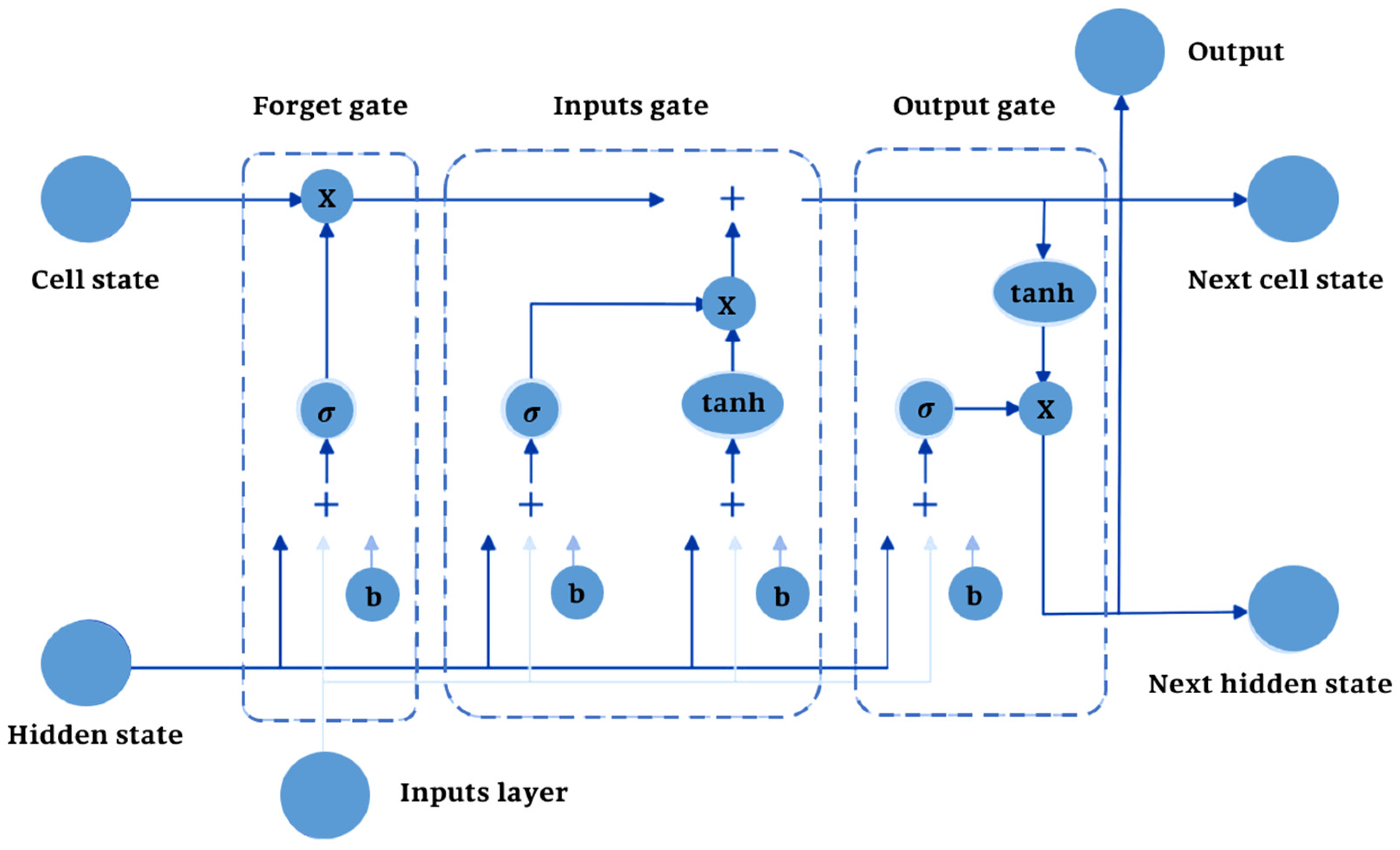
3.2.3. Long Short-Term Memory (LSTM)
LSTM networks are a particular type of Recurrent Neural Network designed to handle the shortcomings of traditional RNNs in capturing long-term dependencies in sequential data. LSTM networks use an entirely new architecture (shown in
Figure 4) to directly handle the vanishing gradient problem and, hence, learn long-term sequences directly [
19,
21].
The key concepts of the LSTM model are its memory cell and gating mechanism. There are three gates for each LSTM unit:
Forget Gate: It regulates what information from the prior time step will be removed from the cell state.
Input Gate: It controls what new information should be added to the cell state.
Output Gate: By using the sigmoid activation function, the output gate is responsible for controlling the output of the memory cell at the current time step, or in determining which information is given to the next layer or time step.
Due to the gating structure, the LSTM can effectively learn to retain or discard information, making it quite powerful for learning temporal dependencies at multiple time scales [
22]. They add nonlinearity and determine how much information flows through the gates by having activation functions like the sigmoid function and the tanh function [
23,
24].
LSTMs are used in applications involving sequence prediction, including time series analysis, speech recognition, machine translation, and video analysis [
22]. Their ability to capture temporal dependencies and adapt to varying sequence lengths makes them a robust tool for a broad range of applications involving complex temporal patterns [
17].
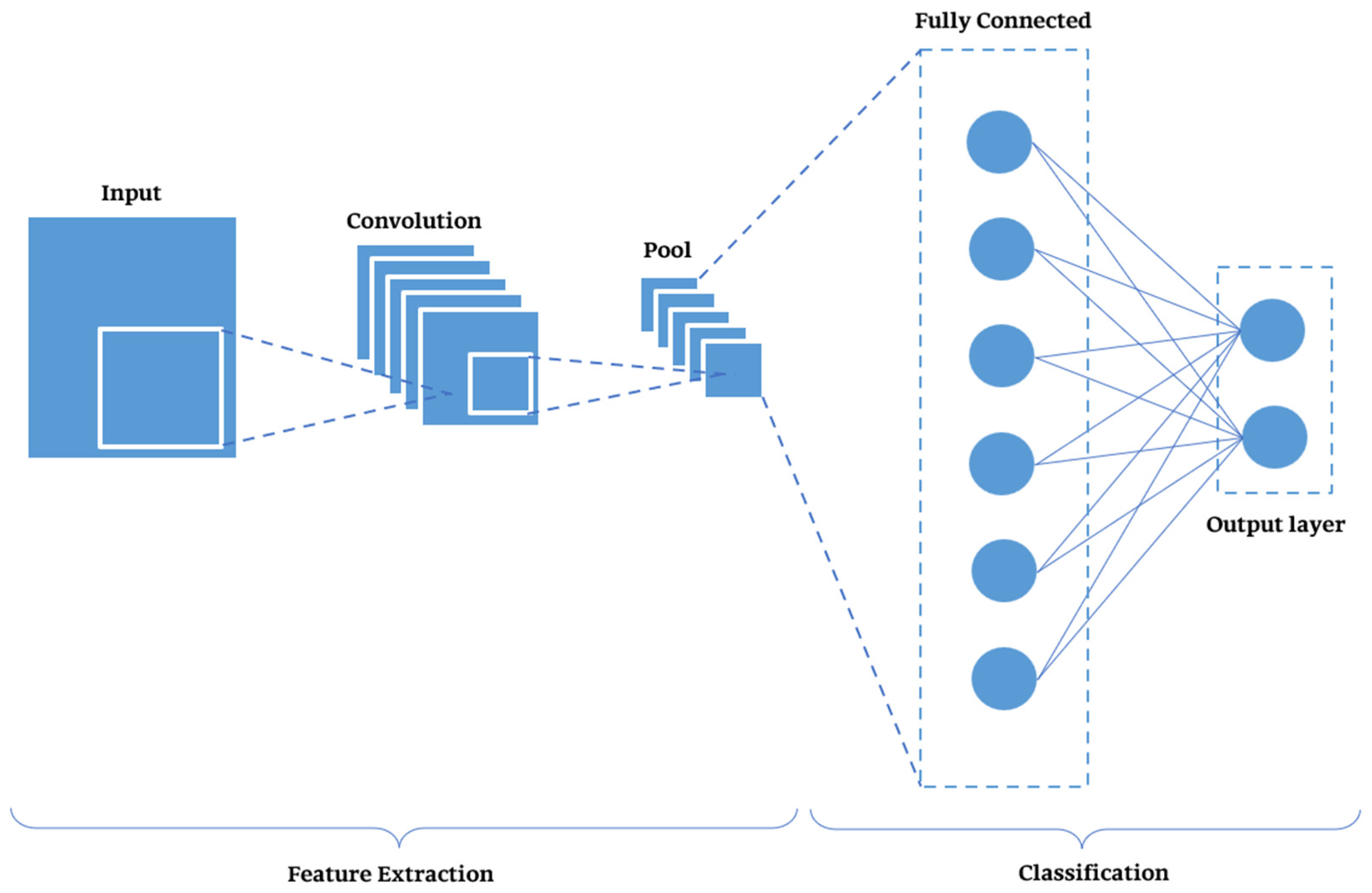
3.2.4. Convolutional Neural Network (CNN)
CNNs are specific types of artificial neural networks that have strong capabilities to handle grid-structured data like images, time series, or structured sensor outputs [
15,
25].
One of the key advantages of CNNs is that, by employing convolutional layers, they learn to extract spatial and hierarchical features automatically, decreasing the dependence on handcrafted features that characterize traditional neural networks [
19,
25].
A CNN consists primarily of three sections (as seen in
Figure 5):
Convolutional Layers: When given an input image, the CNN extracts the features from the image using several convolutional filters. These layers learn to recognize local patterns such as edges, textures, and shapes, which are essential for identifying defects or anomalies in manufacturing scenarios.
Pooling Layers: One of the beginning stages in the neural network, pooling layers, downsample the feature maps, reducing dimensionality by preserving most necessary features, which saves the computational load of the network.
Fully Connected Layers: The extracted features are concatenated to perform the final prediction, such as defect classification or machine failure prediction.
This type of CNN has broad applications for complex datasets when making higher-order decisions and optimizing processes [
26,
27]. The scalability and adaptability of a CNN to a wide range of manufacturing big datasets, multispectral images, vibration signals, or thermal maps are indispensable in industry applications [
27].
3.3. Performance Indicators
Three key metrics have been used in this study to provide a comprehensive picture of the effectiveness and consistency of each of the models. The performance of the trained ML models is based on the analysis of the variance between the predicted and the true data for a variety of measures. The evaluation of the proposed models is carried out using the following indicators: root mean square error (RMSE), mean absolute error (MAE), and R-Squared (R2).
3.3.1. RMSE
The root mean square error (RMSE) is a widespread indicator of measuring how much the predicted values from a model differ from the actual observed values. It is important to note that the RMSE depends on the scale of the data, so it is more useful for evaluating prediction errors within a particular dataset than for comparing different datasets [
28]. The equation for the RMSE is given in (3):
3.3.2. MAE
The mean absolute error (MAE) is a vital metric for evaluating discrepancies between paired observations related to the same event. The MAE is calculated using the following formula, as outlined in Equation (4):
The mean absolute error is calculated on the same scale as the data. However, it should be noted that, as this accuracy metric is dependent on the scale in question, it is not suitable for comparing series with different scales. In the field of time series analysis, the mean absolute error is a common metric used to assess forecast accuracy.
3.3.3. R2
R
2 is the goodness-of-fit metric, which measures the model’s ability to accurately predict data outcomes. It has a range between 0 and 1. Higher values indicate a stronger fit, suggesting that the model performs better [
29]. The following Equation (5) calculates this indicator:
4. Experimentation and Results
This section presents the experimentation and results of the study. It begins with an overview of the dataset, detailing the dataset-associated features, followed by an analysis of the performance of each model. Finally, a comprehensive comparative evaluation is conducted to assess the overall efficacy of the models.
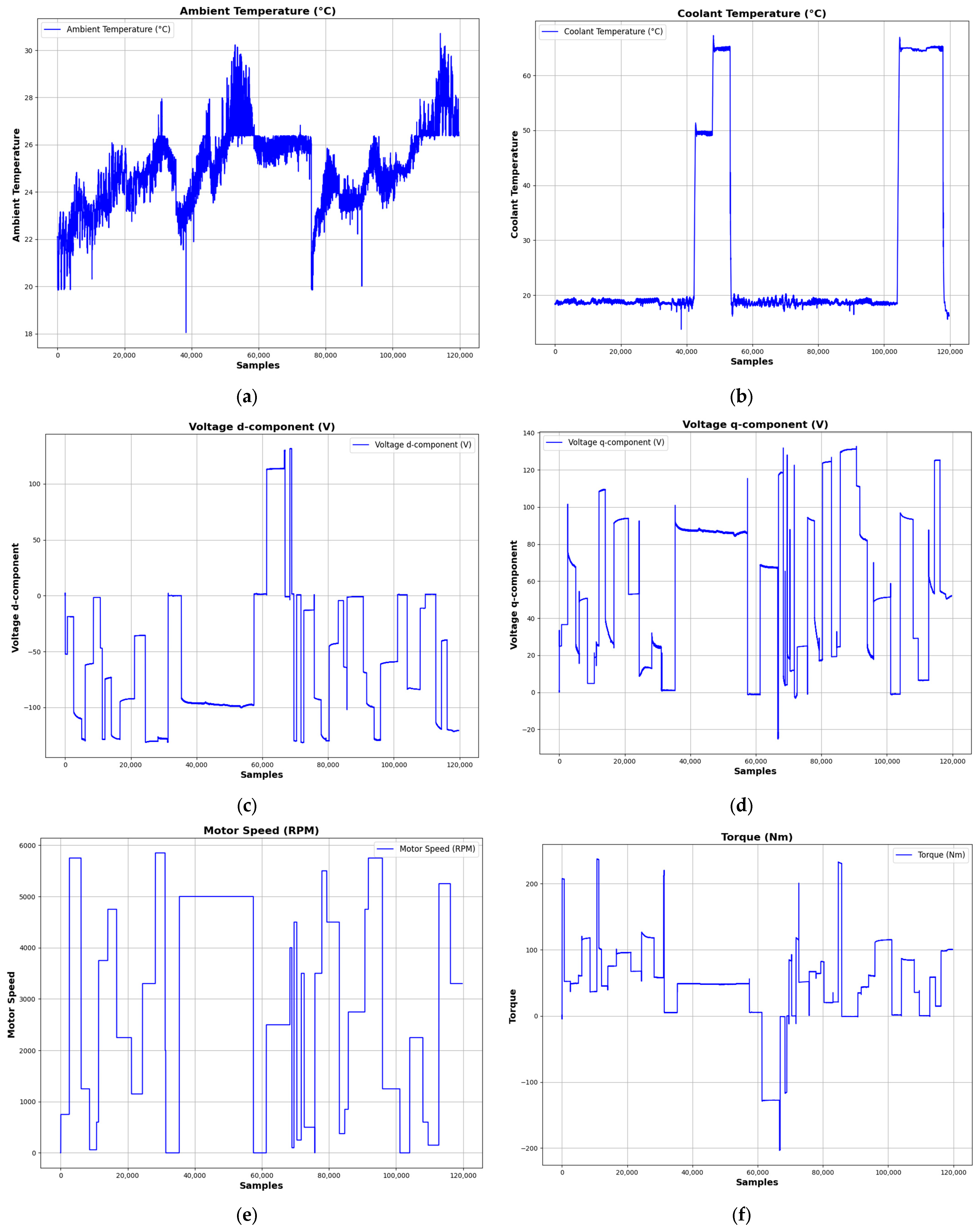
4.1. Dataset Overview
The dataset used in this study is sensor data over a prototype PMSM developed by a German original equipment manufacturer (OEM). The data were collected from a testing experiment performed in the LEA department at Paderborn University [
30]. These recordings measured the motor performance for different operating conditions with a sampling frequency of 2 Hz. The measurements in sessions are between one and six hours long and can be identified by the column “
profile_id”.
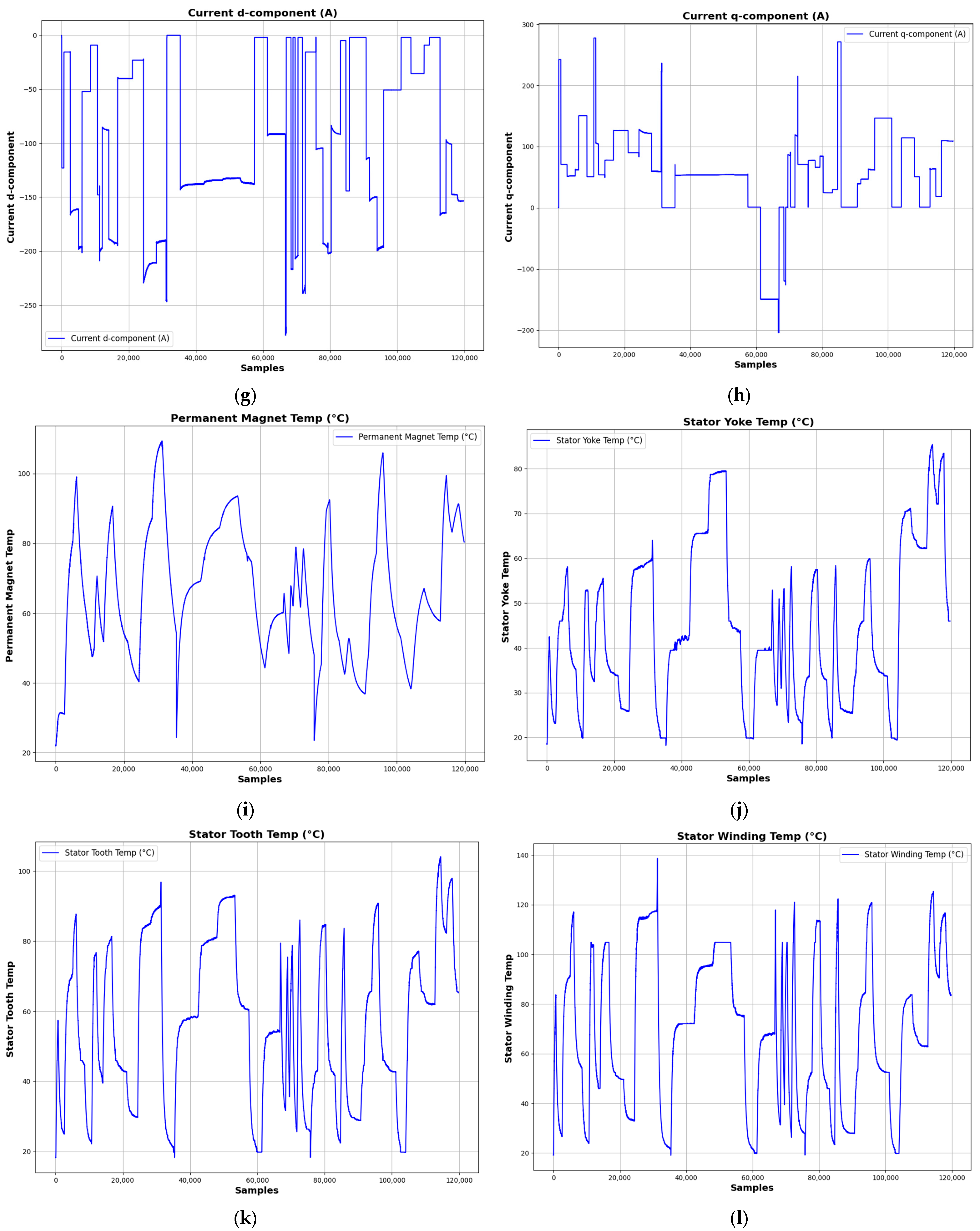
In the process, the motor was driven according to specifically designed cycles of reference values of motor speed and torque. Such driving cycles attempt to closely approximate those occurring in an on-road environment rather than simple ramp-up or steady-state excitations. The currents and voltages in the d/q-coordinates (“i_d”, “i_q”, “u_d”, and “u_q”) were varied in order to change the motor’s speed and torque as an integral part of the control approach. This immediately reflects in the resulting outputs of “motor_speed” and “torque”.
Table 1 depicts the key characteristics.
Figure 6 illustrates a random sample of 120,000 entries from this dataset.
4.2. Performance Analysis of Models
The specifications of the computer used in the experiment are listed in
Table 2. Moreover, the programming language used was Python 3.8.3.
The optimal model performance could be achieved only by a well-implemented, systematic grid search through all the combinations of the predefined hyperparameters, such as the number of layers, neurons in each layer, batch size, learning rate, and type of activation functions. In such a way, it was feasible to check every combination and make a comparison for the selection of the best configuration for each model. The struggles were in the training loss convergence, divergences, instability, overfitting, and the vanishing gradient problem during the training phase, mainly concerning the RNN and LSTM models. Advanced optimizers were employed to make sure that vanishing gradient issues were avoided, while techniques for regularization, means of dropout layers, and cross-validation prevented overfitting. For instability, the tuning of inappropriate learning rates was necessary. Minimizing the loss fluctuation could be achieved by normalizing data and optimizing the batch size. The whole process allowed for the enhanced model to be robust, accurate, and with improved generalization capability.
4.2.1. Results with MLP
An MLP model was used as a baseline for the prediction task (
Table 3). The results of hyperparameter tuning showed that a 128-node, single-layer MLP with the learning rate set to 0.001 gives the best performance. Minimizing divergences with the Adam optimizer allowed the model to achieve a good trade-off of complexity versus generalization.
4.2.2. Results with RNN
The RNN model had the best performance with 64 units by using the Adam optimizer and learning rate of 0.001 for a mean absolute error (MAE) of 1.58, a root mean square error (RMSE) of 2.27, and a coefficient of determination (R
2) of 0.98. Fewer unit configurations (like 32) or a lower learning rate of 0.0005 resulted in non-optimal performance. On the other hand, slow convergence and stability issues contributed toward the 1000-fold regression of stochastic gradient descent (SGD) method. The results showen in
Table 4 depicts the effectiveness of Adam optimizer, highlighting the importance of fine-tuning hyperparameters to achieve the best performance of the model.
4.2.3. Results with LSTM
The LSTM model achieved its best performance with 128 units, a learning rate of 0.001, and a batch size of 32, resulting in the lowest RMSE (1.72) and highest R
2 (0.99). The configurations with the learning rates of 0.001 (128 and 64 units) performed comparably, with slightly higher RMSE and MAE values. These results as presented in
Table 5, emphasize the LSTM model’s strong predictive capability, particularly when tuned with an optimal balance of units and learning rates.
4.2.4. Results with CNN
The CNN model performed best with 64 filters, a learning rate of 0.001, and a batch size of 64, achieving the lowest RMSE of 2.30 and the highest R2 value of 0.98. A small reduction in the learning rate to 0.0005, while keeping the number of filters unchanged, resulted in a slight drop in performance. On the other hand, reducing the number of filters to 32 resulted in an increase in RMSE to 2.78 and a decrease in R2 to 0.97, highlighting the importance of using an adequate number of filters and a well-tuned learning rate for optimal results.
Table 6 illustrates more insights about the CNN model performance.
4.2.5. Execution Time
After applying the grid search methodology to each model, the optimal hyperparameter combination was selected based on performance metrics. However, the execution time remains a cornerstone factor in evaluating the efficiency of our models.
Table 7 presents the execution time corresponding to each model, providing a comparative assessment of computational efficiency.
The performance of the models reveals significant differences in computational cost due to the different architectures. The MLP demonstrates the fastest execution time at 248.46 s, making it the most computationally efficient model in the study. Secondly, we find that the RNN performs slightly higher than the MLP, with an execution time of 264.69 s. The CNN records an execution time of 259.43 s, indicating that its feature extraction process does not significantly increase the computational cost. Conversely, the LSTM (Long Short-Term Memory) has the highest execution time at 436.51 s, reflecting its increased complexity due to memory cell operations and gating mechanisms designed for long-term dependencies.
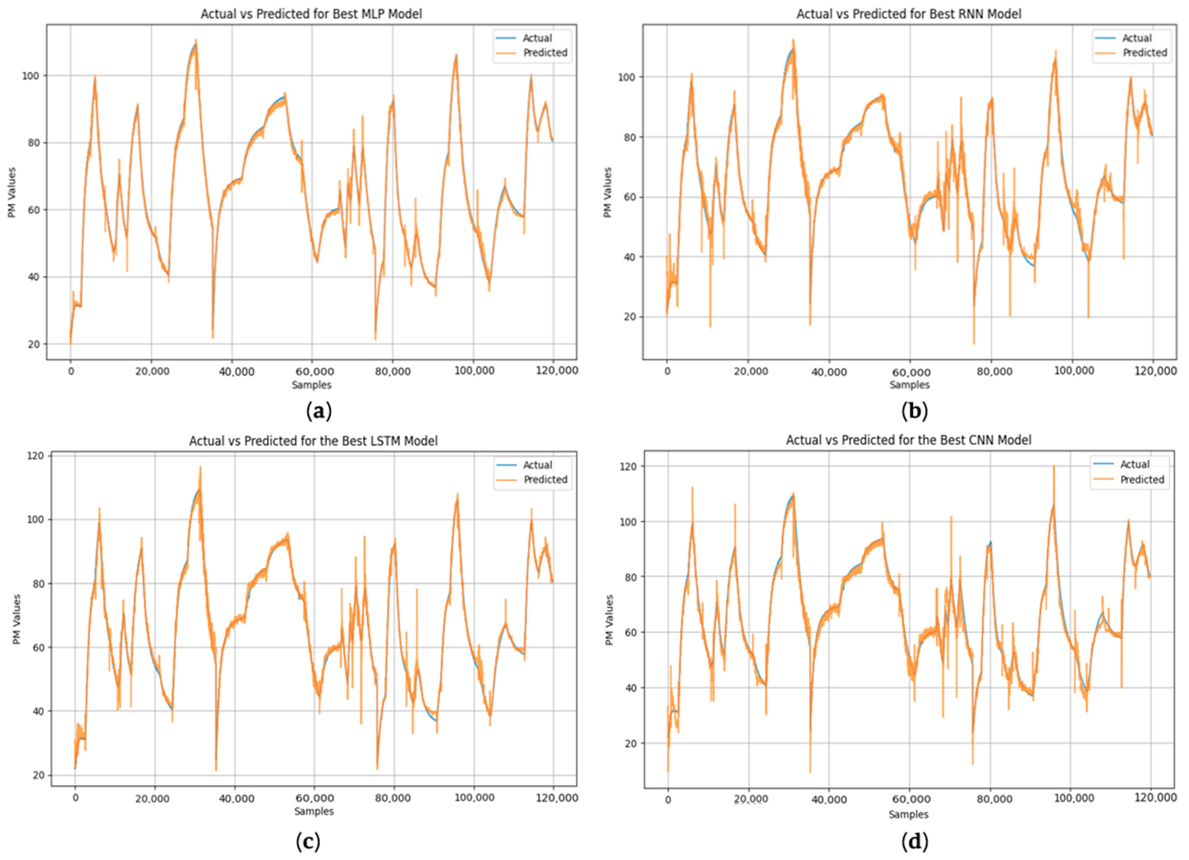
The subsequent figure (
Figure 7) illustrates the comparison between the actual and predicted data across a dataset of 120,000 samples, emphasizing the models’ proficiency in approximating the target output: Permanent Magnet Temperature (“
pm”). This graphical representation offers a comprehensive evaluation of prediction accuracy and demonstrates the degree to which each model aligns with the anticipated values.
4.3. Comparative Evaluation
The assessment of the performance efficacy of our ANN-based models, namely MLP, RNN, LSTM, and CNN, employs three commonly recognized regression metrics (
Section 3.3). The study utilizes optimized hyperparameter settings for each model to facilitate an equitable comparison of their predictive performance.
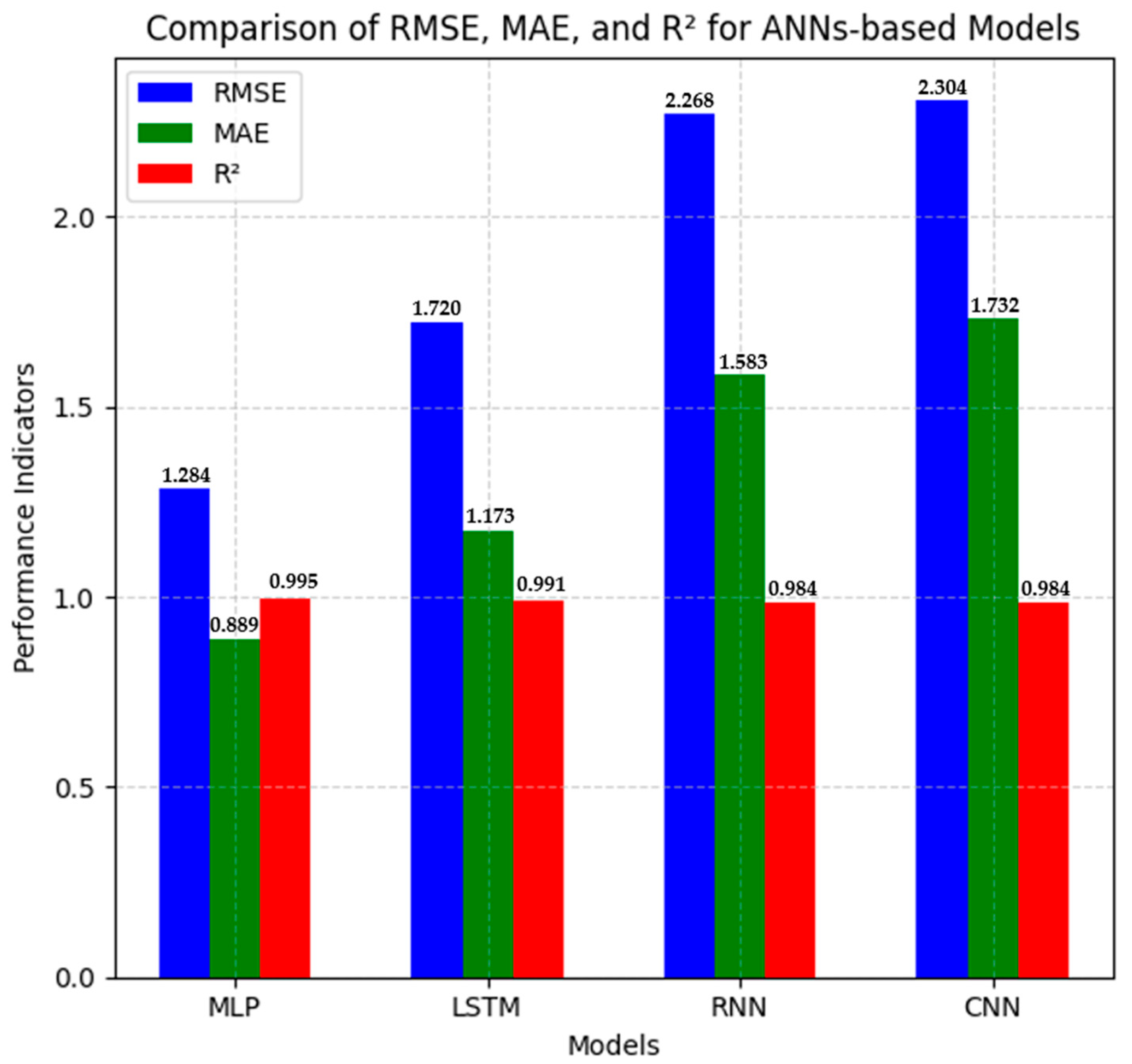
Of these, the MLP model gave the best performance for all metrics: lowest error rates, with RMSE = 1.284 and MAE = 0.889, and highest explanatory power, with R2 = 0.995. These results support the fact that the feedforward architecture of the MLP, together with its optimized configuration, effectively modeled the underlying patterns of the data, and the model predictions showed minimal deviation from the observed ones. Trained on temporal dependencies, the LSTM model ranked second, with a moderate error level (RMSE = 1.720, MAE = 1.174) but with a strong R2 of 0.991. Although this model had slightly worse performance compared to MLP, its inherent ability to process sequential data allows it to stand out for the time-series or context-dependent tasks.
However, both the RNN and CNN architectures were relatively weaker. The RNN resulted in higher errors—a respective RMSE of 2.269 and MAE of 1.584 and a lower R2 score of 0.984, probably due to challenges in modeling long-term dependencies, which is one of the well-known limitations of vanilla RNNs. Similarly, though efficient in handling spatial data, the CNN underperformed in this context: the RMSE was 2.305, while the MAE was 1.733, with an R2 value of 0.984. This might reflect a mismatch between the grid-based feature extraction mechanism of CNNs and the structure of the data, which lacks inherent spatial hierarchies.
Figure 8 presents the relative performance of the four models, arranged from left to right on the X-axis, against the performance metrics, namely RMSE, MAE, and R
2, on the Y-axis.
5. Discussion
This work investigates the predictive performance of four categories of ANN architectures, namely MLP, RNN, LSTM, and CNN. With the basic statistical measures of RMSE, MAE, and the R2 coefficient of determination, an analysis is conducted to depict accuracy and computational efficiency and the practical relevance of the model.
From this comparison, the MLP model had the lowest RMSE and MAE results, suggesting its better capability to decrease error and improve the predictions. On the other hand, the CNN and RNN models had larger RMSE values, indicating relatively less accuracy in predicting temperature. However, their R2 values were similar, indicating that these models can still explain important trends in the data, even if they have larger error margins. Compared to other works published, the findings support well-documented research that has highlighted the high performance of MLP architecture when dealing with time-series forecasting problems for datasets of moderate complexities.
These results are in line with the literature; MLP architectures outperform other models tested on time-series prediction tasks with moderate complexity. In contrast, the results show that LSTM and RNN models are a preferred choice for sequential data modeling, but their performance relies upon hyperparameter tuning, dataset properties, and feature selection strategies. Commonly used in computer vision problems, the CNN model also exhibited relatively moderate prediction strength in this investigation, but its statistically higher RMSE reflects the need for a more sophisticated model in order to excel in predicting time-series outputs.
The MLP model not only obtained the best accuracy but also had the shortest computation time, making it a viable choice for use in real-world predictive maintenance frameworks.
On the other hand, training and inference by the LSTM and RNN models took an extensive amount of time, probably because of their sequentially dependent nature and dependence on past states, which increases their complexity. CNN gave moderately effective performance in regard to prediction but was very computationally expensive since convolutional operations are usually optimized for spatial data, not time series prediction. The results indicate a trade-off between model complexity and computational efficiency, which is an important factor for real-time industrial applications.
This study demonstrates the dominance of the MLP algorithm, presenting a consistent model to use when it comes to simpler scenarios in which temporal or spatial complexity is limited, with the superior abilities of both predictive accuracy and computational efficiency compared with RNNs and LSTMs.
6. Conclusions and Outlook
The promising performance of the MLP model in predicting Permanent Magnet Temperature opens new avenues toward the improvement of predictive maintenance strategies within digital twin frameworks for PMSMs. These low values of the metrics for the model, combined with its computational efficiency, make the model a strong candidate for real-time integration within industrial digital twins. If this model is embedded in the architecture of the digital twin, eventually, the operators will have the potential capability of continuous high-fidelity monitoring of PMSM thermal behavior, the early detection of anomalies such as overheating and risk of demagnetization, and proactive maintenance intervention. Coupling MLP-based temperature prediction with real sensor data streams at runtime, including current, voltage, and rotor speed, constitutes a very crucial step within a digital twin. In this regard, dynamic calibration under different operation conditions would, therefore, be possible, wherein the model attunes itself in case of big fluctuations in the load or sudden environmental stressors. Coupling temperature predictions with physics-based models of motor degradation, such as insulation wear and magnet aging, could further refine failure prognostics, thereby transforming the digital twin into a decision-support tool for maintenance scheduling or operational parameter optimization.
Nevertheless, scaling up the latter for industrial deployment still comes with challenges: first, seamless data synchronization across physical motors with their digital counterpart(s) will require strong IoT infrastructure with minimal latency; second, the validation of the model’s generalizability to larger variations in both design and operating contexts to prevent the model from overfitting to a particular dataset will be necessary; third, building in explainability features—for instance, attention mechanisms or uncertainty quantification into an MLP architecture—is indispensable for creating trust among the operators, more so in safety-critical applications.
Future research needs to be conducted in these hybrid architectures that will marry the efficiency of the MLP with domain-specific enhancements. For instance, federated learning can enable collaborative model training across distributed PMSM fleets to achieve better generalization without compromising data privacy, while edge computing frameworks can decentralize the inference tasks to reduce reliance on cloud infrastructure and improve real-time responsiveness.
From an industrial point of view, this meets the goals of Industry 4.0, such as predictive analytics and autonomous systems. Embedding MLP-driven insights into the digital twin will enable industries to shift away from reactive maintenance strategies toward condition-based ones, reduce unplanned downtime, and extend motor lifespan. Furthermore, the MLP model fits well in these resource-constrained environments, such as offshore wind turbines or electric vehicles, thanks to the smaller computational overhead; real-time processing becomes important here.
Accordingly, the integration of MLP-based temperature forecasting into the PMSM digital twin brings a tremendous leap toward intelligent condition-based predictive maintenance.


 ,
, 


